1.1  Background and Motivation

Quantum Chromodynamics is now well established as the fundamental theory of the strong interaction. The quark model which it is based on provides the basis of our understanding of matter. The description of the quarks’ interaction by the gauge theory that is quantum chromodynamics has been successfully applied to a very wide range of problems. This interaction varies smoothly between the two extremes of confinement, which makes it impossible to isolate quarks, and asymptotic freedom, which makes the quarks inside scattering hadrons behave like free particles at small distances.

Considering how successful and how satisfactory in view of the aim to understand nature from first principles QCD is, it is not surprising that it has eclipsed the attempts to describe the strong interaction which preceded it. One of those is Regge theory [regge1, regge2, collins]. It is based on Lorentz invariance, unitarity and analyticity of the scattering matrix. Developed before quarks and gluons were recognised as the fundamental degrees of freedom of the strong interaction, it is a theory of hadrons. It has been quite successful in describing hadronic scattering processes in the so-called Regge limit, for asymptotically large energies and momentum transfers of the order of a hadronic mass scale.

In Regge theory, the exchange of particles in a scattering process is described by the singularities of the scattering amplitude in the complex angular momentum plane, the so-called Regge poles and cuts. By way of crossing symmetry, they can be related to the masses and spins of existing hadrons. By that token, every hadron is a Regge particle, or Reggeon. However, some Reggeons do not correspond to any known hadrons. One such is the pomeron which is the pole with the largest real part and therefore dominant at asymptotically high energies. It carries the quantum numbers of the vacuum, and the simplest model for it consists of two gluons in a colour singlet state [low, nus]. Another is its charge-conjugation-odd partner, the odderon [lunic]. There are some indications that both pomeron and odderon might be related to glueballs.

To this day, concepts of Regge theory are used widely both in phenomenology, eg [jarbkp, jar, dlfit, gln, dlnew] and theory, eg [gribov, baker, bronsug, fadlip, lipglla, fadintegr, pesch]. The existence of the pomeron is universally accepted, and it is the topic of a wide range of phenomenological work, for instance [dlcond, dlnew, brandt, biapesch, nextbfkl, kharlev, munnav, kharkolev, stasto]. The odderon, by contrast, has never been measured experimentally beyond doubt and consequently is still a contentious topic. A brief overview of odderon physics will be given in the following; for an in-depth review, I refer the reader to [oddreview]. There are few processes in which the odderon is the dominant or indeed only contribution. One such process is the diffractive photo- or electroproduction of $\eta_{c}$ or other heavy pseudoscalar mesons at HERA [kwie_impac, bbcv, engeletac]. But the cross-sections are estimated to be too small to measurable in the foreseeable future. Another odderon-dominated process is the production of light pseudoscalar or tensor mesons, the cross sections for which are expected to be higher [knmeson, rysmeson, msvmeson, msvmeson2]. But it has not been observed experimentally [olsmeson, goldipl, berndt, berndtphd]. This discrepancy might be due to difficulties with the non-perturbative models which are required to describe effects at such low scales.

However, the processes on which the search for the odderon has concentrated for a long time are proton-proton and proton-antiproton scattering, a fact which the large number of publications on the topic attests, for instance [dlfit, gnldlcrit, gln, oddpoint, lev, des, bergnacht, leadtrue, desdips]. These processes provide the hitherto only experimental evidence for the odderon. The elastic differential cross sections of these two processes differ qualitatively: In proton-proton scattering, it shows a dip structure at a squared momentum transfer $t$ of about $t=1$ GeV${}^{2}$, while in proton-antiproton scattering, it only flattens off at this point. Odderon exchange can account for this difference since it carries odd charge conjugation parity and hence contributes with different signs to both processes. What is more, the odderon is the dominant $C=-1$ contribution arising from Regge theory. It is expected to have a Regge intercept of slightly below 1, while $C$-odd meson trajectories typically have intercepts of around 0.5. Since the scattering amplitude of a Reggeon exchange with intercept $\alpha_{0}$ is proportional to $s^{\alpha_{0}+\alpha^{\prime}t}$, the latter contribute much less at high energies. This difference in the differential cross sections has been measured at the Intersecting Storage Rings at CERN [bohm, nagy, ama, erhan, break]. The experimental evidence is marred by the fact that the statistics for $\bar{p}p$ scattering is low and that the difference only shows in a few data points (see Section 2.1). A good description of the data in the framework of Regge theory was given by Donnachie and Landshoff [dlfit]. It is characterised by fair accuracy and considerable predictivity, having only a small number of free parameters. A few years later, it was extended [dlfitnew] to higher-energy proton-antiproton data measured at the CERN SPS [bernard, bernard2]. Proton-proton data at even higher energy from the Tevatron [amos] provide no further check on the fit since they do not extend far enough in $-t$ to show the dip. In the Donnachie-Landshoff fit, the odderon-exchange contribution produces the dip in proton-proton and its absence in proton-antiproton differential cross sections. Another description of $pp$ and $\bar{p}p$ scattering is due to Gauron, Nicolescu and Leader [gln]. It uses the so-called maximal odderon which corresponds to a different type of Regge singularity from other odderon contributions. As in the Donnachie-Landshoff fit, the odderon contribution is instrumental in the description of the dip region. However, the maximal odderon itself already shows a rich structure with a dip. One finding of the work presented in this thesis is that each odderon contribution is compatible only with its own fit, that exchanging odderon contributions between fits is not possible (see Section 4.3.3). But no successful description of the data without an odderon has been found so far. A measurable quantity which is more sensitive to odderon exchange than the cross sections is the ratio of the real to imaginary part of the forward scattering amplitude. But also here no evidence for the odderon has been found [augier].

If the thin experimental evidence for the odderon were all there is to it, one might have discarded it as a misguided concept. But other concepts of Regge theory remain very valid today. Furthermore, the odderon can in fact be derived from perturbative QCD. It is described by the Bartels-Kwieciński-Praszałowicz (BKP) equation [bartbkp, kwiebkp, jarbkp]. Odderon exchange amounts to a simultaneous exchange of at least three gluons in a $C=-1$ state. Since such an exchange is clearly possible in QCD, a failure to find the odderon at all would be a heavy blow to QCD. Odderon research in QCD has received a boost from the discovery that the perturbative odderon is equivalent to an integrable model, the XXX Heisenberg model with spin zero [fadintegr, korintegr]. A prime interest in odderon physics has always been the determination of its Regge intercept, see for instance [gauinter2, gauinter, arminter1, arminter2, brauninter, brauninter2]. Since the discovery of an additional conserved charge of the odderon [lipq3], work has concentrated on finding the spectrum of the associated operator [korq3val, korq3val2, maasq3val, vegaq3val, derkq3val]. Recently, this spectrum has been determined both by Korchemsky et al. [korground, korground2] and by de Vega and Lipatov [vegaground]. To date, there are still unresolved differences between the results of the two groups which centre on the question which eigenvalues of the operator are physical. Separately, explicit solutions of the BKP equation have been found by two groups. One, by Janik and Wosiek [wojan, janwo], has an intercept slightly below one ($\approx 0.96$). It is of the general form derived by Lipatov and collaborators [lipodd, glinodd, lipodd2], in which an analytic auxiliary function is left open. The other solution, by Bartels, Lipatov and Vacca [blvodd], has an intercept of exactly one. This means that its contribution to forward scattering would not decrease with energy. The Bartels-Lipatov-Vacca (BLV) solution was contentious at first since it is not of the general form found by Lipatov, at least not with an analytic auxiliary function. But now it looks like being accepted as legitimate by the community. This is not just of academic theoretical interest, nor just a question about a slightly different intercept. Odderon solutions conforming to Lipatov’s general form cannot couple to some scattering particles, for instance a photon fluctuating into an $\eta_{c}$. The BLV odderon, however, can. Therefore, with the advent of this new solution a number of new processes in which the odderon may play a role becomes available.

A solution of the BKP equation, which describes the odderon’s propagation, is only one ingredient for calculating the odderon contribution to a given process. Besides, impact factors describing the odderon’s coupling to scattering particles are required. Pomeron impact factors have always aroused some interest [asaipomimp, klenpomimp, golpomimp] and have just been computed in next-to-leading order [ciapomimp, bartpomimp, giepomimp, fadpomimp]. Less work has been done on odderon impact factors [fk, lev, dloddimp, kwie_impac]. While some impact factors can be calculated perturbatively (for instance the odderon-$\eta_{c}$ impact factor [kwie_impac]), impact factors for proton scattering require non-perturbative ansätze most of which have never been confronted with experimental data. As part of this work, the odderon-proton impact factors of Levin and Ryskin [lev] and Kwieciński et al. [fk, kwie_impac] were used to calculate the elastic differential cross section for proton-proton scattering. The odderon was described simply as three gluons in a $C=-1$ colour singlet state. The non-odderon contributions were taken from the Donnachie-Landshoff fit [dlfit]. This allows to fix the coupling constant to be used with these impact factors. My results imply that predictions of the $\eta_{c}$ production cross section by Kwieciński and two other group using his impact factors [engeletac, bbcv] have to be revised downwards, see Section 3.4.

The main interest of the first part of this thesis (Chapters 2, 3 and 4) is however a different one. It has been known for some time that the structure of the proton has considerable effect on the odderon-proton impact factor. In the extreme case in which two of the proton’s valence quarks are clustered in a point-like diquark, the odderon-proton coupling even vanishes [oddpoint]. The odderon contribution for a diquark cluster of finite size in the proton was computed non-perturbatively by Rüter and Dosch [rueter, rueterphd]. They used it to determine the ratio of the real to imaginary part of the forward scattering amplitude for proton-proton and proton-antiproton scattering, respectively. The perturbative odderon contribution to these processes for a finite-sized diquark is presented in this thesis, in Chapter 2. By computing the differential cross section in the dip region for proton-proton scattering, the average size of the diquark cluster is obtained from experimental data (Chapters 3 and 4). The geometrical nature of the concept of a diquark cluster necessitates the use of a position-space approach to high-energy scattering. I choose the one developed by Nachtmann [nacht], which is otherwise used mainly with non-perturbative models, notably the Model of the Stochastic Vacuum, see for instance [doschmsv, dsmsv, simmsv, dfk, rueter, bergnacht, msvmeson, ssmsv, ssmsv2]. My result of a small diquark size will benefit non-perturbative calculations: Many of them treat the proton as a colour dipole [dfk, bergnacht, ssmsv3], which is legitimate since soft gluons cannot resolve a small diquark.

Important though many results of Regge theory remain in present-day high-energy physics, our understanding of the Regge limit from the first principles of QCD is still far from complete. This is because high-energy hadronic processes tend to involve large parton densities and are dominated by soft scales. Our knowledge of non-perturbative QCD is not yet sufficient for a rigorous treatment of the vast majority of high-energy processes. However, some processes are dominated by one hard scale and therefore allow the application of perturbation theory. One such is the scattering of heavy quarkonia. The process itself is not experimentally feasible. But since photons tend to fluctuate into $q\bar{q}$ states in high energy scattering, the scattering of highly virtual photons is expected to provide a suitable substitute. This is predicted to be measurable [bartvirt1, bartvirt2, bhsvirt1, bhsvirt2] at a future $e^{+}e^{-}$ collider like the planned Next Linear Collider [nlc, nlczdr]. A situation similar to the process just mentioned occurs in the presence of hard forward jets in deep inelastic or in hadronic scattering, called forward jets and Mueller-Navelet jets, respectively [mueljet, muelnav]. They have been investigated in depth by a variety of groups, for example [brljet, kmsjet, tangjet, bartjet2, pestruct, bartjet3, elvjet, munjet, andjet, andjet2, enbjet, bartjet4]. Another process involving a hard scale is deep inelastic electron-proton scattering at small values of the Bjorken scaling variable $x$. In this case the hard scale is provided by the virtual photon which mediates the interaction on the electron’s side.

Even in the presence of a hard scale, perturbation theory in high-energy QCD is not trivial. Due to the large energies available, the phase space of intermediate gluons becomes very large, $\propto\log s$. In QCD, this logarithmic factor can compensate the smallness of the coupling constant, with the effect that more complicated Feynman graphs are not always suppressed. Therefore an infinite number of graphs have to be resummed to obtain a consistent leading-order result. This is called the Leading Logarithmic Approximation. The resummation was performed for the first time in QCD by Balitsky and Lipatov [blbfkl], using earlier work by Lipatov and collaborators [fklbfkl]. The result of the resummation is described by the well-known BFKL equation. The corresponding Reggeon exchange is called the BFKL, perturbative or hard pomeron. It represents a bound state of two reggeised gluons and was found to correspond to a Regge cut in the complex angular momentum plane. A reggeised gluon is a colour octet state composed of several QCD gluons [lipreggluon]. It was discovered in 1985 that the BFKL equation is conformally invariant in transverse position space [bfklconf]. This was a finding of great importance since it allowed the solving of the equation in the non-forward direction. It also led to a novel interpretation of BFKL evolution as a two-dimensional conformally invariant quantum mechanics in which the complexified angular momentum is the energy-like and rapidity the time-like variable.

Since the invention of the BFKL pomeron it has become clear that it violates a basic principle of field theory: unitarity. The Froissart-Martin theorem, derived from this principle, states that hadronic cross sections can rise at most with the squared logarithm of energy. The growth of the BFKL-pomeron-exchange cross section is power-like, with an exponent of $\alpha_{s}4\ln 2N_{c}/\pi\approx 0.5$. But the BFKL pomeron represents only a leading-order approximation. Higher-order corrections tame this power-like growth and restore unitarity.

A complete resummation of higher-order graphs relevant for pomeron exchange is even today thought to be prohibitively difficult. One has to be content with adding specific classes of graphs which are chosen to restore compliance with the Froissart-Martin Theorem and hence unitarity. For restoring the unitarity of the overall scattering matrix one has to add ladder graphs with more than two reggeised gluons in the $t$ channel. These additional terms are called unitarity corrections. The amplitudes (or propagators) of these larger bound states of reggeised gluons are described by the Bartels-Kwieciński-Praszałowicz (BKP) equations [bartbkp, kwiebkp, jarbkp]. They can be greatly simplified by treating only the large $N_{c}$ limit. Then a nearest-neighbour interaction takes the place of the $n$-particle interaction between the reggeised gluons. This amounts to a one-dimensional solid, and was found to be equivalent to the XXX Heisenberg model with spin zero, a completely integrable model [lipq3, lipglla, fadintegr]. This limited approach of demanding unitarity only for the overall process is followed by Lipatov [lipglla].

A more ambitious and more complete approach is due to Bartels [bartglla, bartglla1, bartglla2]. It demands unitarity not just in the main process but also in all possible subprocesses. This requires the inclusion of graphs in which the number of reggeised gluons in the $t$ channel is not constant. Starting from two reggeised gluons coupling to the scattering particles, amplitudes of more than two reggeised gluons emerge. It was found that the three- and five-gluon amplitudes are in fact just superpositions of amplitudes with fewer gluons [bw, carlophd, be], a phenomenon known as reggeisation. The four-gluon amplitude also contains a reggeising part [bw]. But besides that a vertex transforming two to four gluons occurs, which gives rise to a new form of four-gluon amplitude. The conformal invariance of this new vertex was shown in [blw]. The six-gluon amplitude, investigated in [carlophd, be], consists of a completely reggeising part, a partially reggeising part, and a new $2\to 6$ vertex. The completely reggeising part is a superposition of two-gluon amplitudes, the partially reggeising part a superposition of four-gluon amplitudes. The $2\to 6$ vertex again gives rise to a new amplitude. If all transitions to a larger number of reggeised gluons were conformally invariant, these unitarity corrections would amount to a conformal field theory in $2+1$ dimensions. In analogy to the conformal quantum mechanics suggested by BFKL, rapidity would serve as the time-like variable and the complex angular momentum as the energy-like variable.

Recent work [pesch, korconf, conf1_Nc, stringy] suggests an even more intimate connection between string theory/conformal field theory and unitarity corrections. Some of this work involves pomerons as the fundamental degrees of freedom and pomeron vertices. Vertices of BFKL pomerons can be obtained by projection of the reggeised-gluon transition vertices. The simplest of these, transforming one to two pomerons, has been investigated in [lotterphd, pesch, korconf, braun3p, bart3p] and found to have the form of a conformal three-point function. There is some confusion about the existence of higher vertices transforming one to $n>2$ pomerons. Of course higher vertices could be constructed by iterating the $1\to 2$ vertex. But such composed vertices would not be local in rapidity since the intermediate states of pomerons would have to be allowed to evolve. Peschanski [pesch] has given an interpolated expression for local $1\to n$ pomeron vertices which, like the $1\to 2$ vertex, allows an interpretation as string-theoretic Shapiro-Virasoro amplitudes. Since then, Braun and Vacca [brvac] have proven that such local vertices do not exist in the dipole approach of Mueller [mueller, mueller2]. This approach provides a derivation of the BFKL equation which is much easier than the original one involving gluon ladders. However, it is not thought to be equivalent to the gluon-ladder approach to all orders, not least because it does not allow the exchange of an odderon. While Peschanski also starts out from dipoles, the expression he generalises is much closer to the gluon-ladder form of the result obtained by Lotter [lotterphd].

Some of the questions about higher pomeron vertices are addressed in the second part of this work. Chapter 5 consists of preparing the groundwork for treating reggeised-gluon and pomeron vertices in a systematic way. It deals with a function $G$ in terms of which the $2\to 4$ and $2\to 6$ reggeised gluon vertices can be expressed, and its components. The properties of $G$ under conformal transformations prove the conformal invariance of the $2\to 6$ vertex and also of higher vertices if they have an analogous form as suggested in [ew2]. This represents an important step towards proving the existence of a conformal field theory of unitarity corrections. In Chapter 6 the $1\to 3$ pomeron vertex is derived in the gluon-ladder approach and cast into the form of a conformal four-point function. Its existence does not contradict the result of Braun and Vacca but rather reveals a discrepancy between the gluon-ladder and the dipole approach. Their equivalence extends only to the $1\to 2$ pomeron vertex but not to higher orders.

Introduction

1.2 High-energy scattering

When a number of particles get close to each other, they interact, possibly break up and fly off in directions different from that of their initial trajectories. This is called a scattering process. To simplify its description, one assumes that the scattering particles approach each other from a macroscopically large distance, interact in a microscopically small region, and that the products of the interaction move away again to a macroscopically large distance. Before and after the interaction, the particles are thought of as so far apart that they are effectively unaware of each other. The scattering operator $\mathcal{S}$ is defined as the operator which transforms the initial multi-particle state in the infinite past to the final multi-particle state in the infinitely remote future.

$$\halign to=0.0pt{ \hfil$\displaystyle{#}$&\hfil$\displaystyle{{}#{}}$\hfil&$\displaystyle{#}$\hfil&\refstepcounter{equation}\label{#}\llap{(\theequation)}\cr\vskip-6.0pt\cr\lim_{t\to+\infty}|t\rangle=|f\rangle&=&\mathcal{S}\,|i\rangle=\mathcal{S}\,\lim_{t\to-\infty}|t\rangle\crcr}$$

Since the time-evolution operator is linear, so is the scattering operator. In a suitable base, it can therefore be written as a matrix, the scattering matrix, with elements denoted by $\mathcal{S}_{fi}$. More often than $\mathcal{S}$, one uses the $\mathcal{T}$ matrix. It is obtained from $\mathcal{S}$ by subtracting the unit matrix and removing some kinematic factors. It therefore can be thought of as describing the effect of the interaction, since a scattering matrix equal to unity amounts to no interaction.

$$\halign to=0.0pt{ \hfil$\displaystyle{#}$&\hfil$\displaystyle{{}#{}}$\hfil&$\displaystyle{#}$\hfil&\refstepcounter{equation}\label{#}\llap{(\theequation)}\cr\vskip-6.0pt\cr\mathcal{S}_{fi}&=&\delta_{fi} + i\,(2\pi)^{4}\,\delta^{4}(P_{f}-P_{i})\,\mathcal{T}_{fi} \crcr}$$

Here $P_{i}$ and $P_{f}$ are the total four-momenta of all particles in the initial and final states, respectively.

The $\mathcal{T}$ matrix element is also called the scattering amplitude and denoted by $T$. It is not usually expressed as a function of the initial and final states. Rather, kinematic variables which characterise the states are used as arguments of $T$. Easily the most important kinematic variable is $s$. It is the square of the centre-of-mass energy, or equivalently the square of the invariant mass of the scattering system.

$$\halign to=0.0pt{ \hfil$\displaystyle{#}$&\hfil$\displaystyle{{}#{}}$\hfil&$\displaystyle{#}$\hfil&\refstepcounter{equation}\label{#}\llap{(\theequation)}\cr\vskip-6.0pt\cr s&=&P_{i}^{2}=P_{f}^{2} \crcr}$$

In “high-energy” scattering, one treats the limit $s\to\infty$, or in experimental reality the case where $s$ is significantly larger than the squares of all the particle masses, $s\gg m_{n}^{2}\;\forall\,n$.

Figure 1.1: A two-particle to two-particle scattering process.

Let us now turn to the case of two particles scattering and two (possibly different) particles emerging after the scattering process. This situation is displayed graphically in Figure 1.1. The diagram can be read in two ways: from left to right or from top to bottom. The left-to-right view corresponds to the reaction

$$a+b\longrightarrow c+d\,.\qquad\hbox{($s$ channel)}$$

The top-to-bottom view corresponds to the reaction

$$a+\bar{c}\longrightarrow\bar{b}+d\,.\qquad\hbox{($t$ channel)}$$

$b$ and $c$ become antiparticles since they now propagate backwards in time. This process has the centre-of-mass energy $(p_{a}-p_{c})^{2}=:t$. Looking at the the $t$-channel process instead of the original $s$-channel reaction is called “crossing”. There is a third kinematic variable $u$ and a corresponding third process in which it is the squared centre-of-mass energy:

$$a+\bar{d}\longrightarrow\bar{b}+c\qquad\hbox{($u$ channel)}.$$

These three kinematic variables are very important in any of these processes. They are called Mandelstam variables. They are not independent but add up to the sum of the mass squares of the four particles. Here is their definition:

$$\halign to=0.0pt{ \hfil$\displaystyle{#}$&\hfil$\displaystyle{{}#{}}$\hfil&$\displaystyle{#}$\hfil&\refstepcounter{equation}\label{#}\llap{(\theequation)}\cr\vskip-3.0pt\cr s&=&(p_{a}+p_{b})^{2}\cr t&=&(p_{a}-p_{c})^{2}&\hbox to0.0pt{\hss(1.1\cr u&=&(p_{a}-p_{d})^{2}\cr}}$$

In the $s$-channel process, $s$ is the squared centre-of-mass energy. $t$ is the squared four-momentum transfer: If one assumes the particle $a$ to emerge as particle $c$, the four-momentum $p_{a}-p_{c}$ has been transferred to $b$ (which becomes $d$). This is also the negative square of the invariant mass of the (virtual) particle mediating the interaction. One can show that in $s$-channel processes, $t$ is always negative. After crossing, the variables exchange their roles. In the $t$-channel process, $t$ is the squared centre-of-mass energy and $s$ is the squared four-momentum transfer. Now $s$ is negative and $t$ is positive. (It has to be taken into account that in the crossed process, the momentum of $\bar{c}$ is $-p_{c}$.)

Interestingly, the same scattering amplitude applies in all crossed processes. It just has to be continued analytically to the region in which the Mandelstam variables have the right sign for the desired channel. This is called crossing symmetry.

Let us now turn from kinematics to calculating observables for $s$-channel processes. The observables of most universal interest are cross sections. The most widely used differential cross section is the derivative of the cross section with respect to $t$. It is easily computed from the scattering amplitude:

$$\halign to=0.0pt{ \hfil$\displaystyle{#}$&\hfil$\displaystyle{{}#{}}$\hfil&$\displaystyle{#}$\hfil&\refstepcounter{equation}\label{#}\llap{(\theequation)}\cr\vskip-6.0pt\cr\mathinner{d\sigma \over dt} &=&\mathinner{T(s,t)^{2} \over 16\,\pi\, s^{2}}\,. &\hbox to0.0pt{\hss(1.2\crcr}}$$

The total cross section could of course be obtained by integrating over the differential cross section. But there is a simpler way which makes it possible to obtain it directly from the scattering amplitude. This is by using the optical theorem. It is a special case of the Cutkosky rules and relates the forward elastic scattering amplitude to the total cross section. In the high-energy limit, the optical theorem has the following form:

$$\halign to=0.0pt{ \hfil$\displaystyle{#}$&\hfil$\displaystyle{{}#{}}$\hfil&$\displaystyle{#}$\hfil&\refstepcounter{equation}\label{#}\llap{(\theequation)}\cr\vskip-3.0pt\cr 2\,\hbox{Im}\,T(s,0)&=&2\,s\,\sigma_{tot}(s)\,. &\hbox to0.0pt{\hss(1.3\crcr}}$$

This allows to compute the total cross section.

1.3 The standard model, the strong interaction and QCD

The standard model is a description of the three interactions relevant in elementary particle physics — the electromagnetic, weak and strong interaction. This description is based on quantum field theory.

The electromagnetic and weak interactions are jointly described by the Weinberg-Salam model. It is basically a gauge theory with four massless gauge bosons and a scalar particle, the Higgs. By fixing the vacuum expectation value of the Higgs field, one induces spontaneous symmetry breaking. As a consequence, a gauge theory with three massive ($W^{\pm}$, $Z^{0}$) and one massless ($\gamma$) gauge bosons emerges. Even though the Higgs boson has not yet been detected, this model is very successful.

The strong interaction is described by quantum chromodynamics (QCD). Its foundation is the quark model, the idea (supported by experiment) that hadrons are composed of smaller point-like particles which cannot be isolated, the quarks. Quarks have two quantum numbers peculiar to them: flavour (which accounts for different types of hadrons) and colour (which is the gauge charge of QCD). There are three different colours, and to date six flavours of quarks have been found. Observable particles are superpositions of systems of quarks of all three colours, which renders them colour-neutral, “white”. The gauge bosons of QCD are called gluons. They are massless and come in the eight existing colour-anticolour combinations, excluding white.

Making predictions on the basis of QCD is much harder than in QED, for two reasons: One, gluons couple to each other. There is a three-gluon and a four-gluon vertex in QCD. Two, QCD exhibits confinement. The most obvious effect of this property is that colour-carrying particles cannot be isolated. Its deeper reason is that the strong coupling constant is large at small momenta. (Correspondingly, it is small at high momenta, which is called asymptotic freedom.) Taken together, these two points mean that gluons have a tendency to split up into more gluons (or quark pairs) and that more complicated Feynman graphs are not always significantly suppressed.

Problems concerning the strong interaction at low energies cannot be solved with perturbative QCD. Additional models or lattice calculations are required. Perturbation theory does not work at low energies. Perturbative calculations of the evolution of the strong coupling constant lead to a divergence at the scale $\Lambda_{\rm QCD}\approx 250$ MeV. The expression for this evolution probably starts to lose its meaning below two to four times that value. Non-perturbative QCD is not the topic of this thesis, but the limitations of perturbation theory have to be kept in mind in any QCD calculation.

1.4 Before QCD: Regge theory

1.4.1 Regge theory and the scattering matrix

Before the development of QCD as a quantum field theory of the strong interaction, attempts were made to derive the properties and behaviour of hadrons from reasonable assumptions about the scattering matrix. The resulting theory is called Regge theory after its inventor, T. Regge [regge1, regge2]. (See [collins] for a thorough treatment.)

The assumptions about $\mathcal{S}$ are the following:

1. $\mathcal{S}$ is Lorentz-invariant. We have already made this assumption in the first section when we wrote the scattering amplitude as a function of the Lorentz invariants $s$ and $t$.

2. $\mathcal{S}$ is unitary, $\mathcal{S}\mathcal{S}^{\dagger}=\mathcal{S}^{\dagger}\mathcal{S}=\hbox{$1\hskip-1.2pt\vrule depth=0.0pt,height=6.88889pt,width=0.7pt\vrule depth=0.0pt,height=0.3pt,width=1.19995pt$}$. This is the conservation of probability, ie the probability for a specific initial state to end up in any final state at all must be one.

3. $\mathcal{S}$ depends analytically on Lorentz invariants. Unitarity takes precedence over this, ie singularities which are necessary for unitarity are allowed.

The last point requires some explanation. It may seem strange that unitarity requires singularities in the scattering amplitude. The reason lies in the optical theorem (1.2) which relates the forward elastic scattering amplitude with the total cross section. The Cutkosky rules from which it is derived are a consequence of unitarity of the $\mathcal{S}$ matrix. By way of the optical theorem, contributions to the total cross section (from any reaction) relate to contributions to the imaginary part of the forward elastic amplitude. Therefore one can learn something about the scattering amplitude by looking at all the final states which might arise from two scattering particles.

Two particles can merge into one only at discrete energies. They can create two different particles only at energies higher than the combined mass of the lightest pair of particles allowed by quantum number conservation. Therefore there are intervals on the real $s$ axis where the total cross section, and therefore the imaginary part of the forward scattering amplitude, is zero. This allows to apply the Schwarz reflection principle from the theory of complex functions: When a function is analytic in a given domain and real on a straight line contained in that domain, then it takes values which are complex conjugates of each other at points which are mirror reflections with respect to that line. In this context this means that

$$T(s^{*},t)=T(s,t)^{*}$$

in its domain of analyticity. (The straight line is one of the intervals on the real $s$ axis where $T$ is real, so the mirror image of $s$ is $s^{*}$.)

Figure 1.2: Singularity structure of the scattering amplitude in the $s$ plane. It is symmetric to a line parallel to the imaginary axis, but not necessarily to the axis itself.

Since an analytic function has a unique power expansion in its domain of analyticity, $T$ would have to be real on the whole real $s$ axis if it were to be analytic there. But that would mean $\sigma_{tot}=0$ for all energies, which is clearly not usually true. Therefore $T$ has to be singular at large parts of the real axis. The non-zero multiple-particle production amplitudes are represented by branch cuts (since they extend all the way to infinity from the $n$-particle-production threshold), while single particle production is represented by isolated singularities, usually poles. It can be shown from crossing symmetry and the relation between the Mandelstam variables that $T$ has a structure symmetric with respect to a parallel to the imaginary axis, so that the singularity structure shown in Figure 1.2 emerges.

1.4.2 Complex angular momenta

Let us consider two-particle to two-particle scattering. It is well known from quantum mechanics that one can express the scattering amplitude in terms of the spherical harmonics with zero angular momentum, $Y_{l,0}$, which are Legendre polynomials in the cosine of the scattering angle, $\cos\theta$. This is called partial wave expansion. In the $s$ channel, $\cos\theta=1+2s/t$ and one can write:

$$\halign to=0.0pt{ \hfil$\displaystyle{#}$&\hfil$\displaystyle{{}#{}}$\hfil&$\displaystyle{#}$\hfil&\refstepcounter{equation}\label{#}\llap{(\theequation)}\cr\vskip-6.0pt\cr T(s,t)&=&\sum_{l=0}^{\infty}(2l+1)\,a_{l}(s)\,P_{l}(1+2s/t)\,, &\hbox to0.0pt{\hss(1.4\crcr}}$$

where $a_{l}$ are the coefficients of the expansion, the partial wave amplitudes. This expression can be rewritten according to Cauchy’s integral theorem as a contour integral in the complex $l$ plane over a function with singularities at $l\in\mathbb{N}_{\geq 0}$. The value of the integral is the sum of the residues at these poles, which are constructed to equal the terms in the sum in (1.4.2). This is called Sommerfeld-Watson transform. One obtains:

$$\halign to=0.0pt{ \hfil$\displaystyle{#}$&\hfil$\displaystyle{{}#{}}$\hfil&$\displaystyle{#}$\hfil&\refstepcounter{equation}\label{#}\llap{(\theequation)}\cr\vskip-6.0pt\cr T(s,t)&=&\oint dl\, \mathinner{1 \over\sin\pi l}\, (2l+1)\,a(l,s)\,P(l,1+2s/t)\,. &\hbox to0.0pt{\hss(1.5\crcr}}$$

The integration contour extends to infinity and circles the positive real axis clockwise. The argument $l$ of $a$ and $P$ is no longer written as an index to indicate that it is a now complex variable and that these functions have been analytically continued over the whole complex $l$ plane.

The analytic continuation of the partial wave amplitude $a$ is not unique. Adding a function with zeros at all non-zero integers to it does not change the integral. But such a function has to be a sine with a period of two divided by an integer. Such a sine function would rise exponentially on the imaginary axis. So there is a unique $a(l,s)$ which rises more slowly than $\exp(\pi|l|)$ as $l$ approaches infinity. However, some contributions to the partial wave amplitude oscillate as $(-1)^{l}$. This would be analytically continued to a cosine, which also rises faster than our limit. Since adding a sine function cannot correct that on both the positive and negative imaginary axis, a different route is chosen. The analytic continuation is done for even and odd angular momenta separately, and $a(l,s)$ is replaced by

$$\halign to=0.0pt{ \hfil$\displaystyle{#}$&\hfil$\displaystyle{{}#{}}$\hfil&$\displaystyle{#}$\hfil&\refstepcounter{equation}\label{#}\llap{(\theequation)}\cr\vskip-6.0pt\cr\tilde{a}(l,s)&=&\sum_{\eta=\pm 1}\mathinner{1 \over 2}\,(\eta+e^{-i\pi l})\,a^{(\eta)}(l,s)\,. \crcr}$$

$\eta$ is called the signature of the partial wave.

To investigate the form of the scattering amplitude in the high energy (Regge) limit, one transforms the integration contour so that the contour integral vanishes in this limit. What remains are the residues of the integrand’s poles the contour swept over during the deformation. These are called Regge poles. Using an asymptotic formula for the Legendre polynomials, one obtains for each of the poles a contribution

$$\halign to=0.0pt{ \hfil$\displaystyle{#}$&\hfil$\displaystyle{{}#{}}$\hfil&$\displaystyle{#}$\hfil&\refstepcounter{equation}\label{#}\llap{(\theequation)}\cr\vskip-6.0pt\cr T(s,t)&\propto&s^{\alpha(t)}\,, &\hbox to0.0pt{\hss(1.6\crcr}}$$

where $\alpha(t)$ is the pole’s position in the complex $l$ plane depending on $t$. In view of this form, one can say that at high energies the scattering amplitude is dominated by the Regge pole with the largest real part. The expression (1.4.2) is usually interpreted as the exchange of a “Reggeon”, an object with angular momentum equal to $\alpha(t)$. $\alpha(t)$ is called its Regge trajectory.

To gain some understanding of Regge trajectories, one continues them to the region $t>0$. It was found that mesons plotted in a diagram of angular momentum against square mass are arranged in straight lines. Based on this fact it is usually assumed in Regge theory that Regge trajectories are linear functions also for $t<0$, that is

$$\alpha(t)=\alpha_{0}+\alpha^{\prime}t\,.$$

$\alpha_{0}$ is called a Reggeon’s Regge intercept, $\alpha^{\prime}$ its Regge slope. From (1.4.2) one derives that the differential cross section for a process in which a single Reggeon is exchanged is

$$\mathinner{d\sigma\over dt}\propto s^{2\alpha_{0}+2\alpha^{\prime}t-2}\,.$$

1.5 Pomeron and odderon

Both pomeron and odderon are not particles but “objects” which can be exchanged in scattering processes. They are well described by Regge theory, and hence are Reggeons. This section will give a brief introduction to them and to how to understand them in terms of QCD. For a detailed treatment see [fr] or [ddln]. The state of the art of odderon research has been reviewed very recently in [oddreview].

The existence of the pomeron is universally accepted nowadays. It is based on the following path of reasoning: The Pomeranchuk theorem [pomtheo] states that total cross sections of scattering processes in which charged particles are exchanged have to vanish asymptotically for high energy. Here, “charge” can mean any kind of charge, including electric charge, isospin, colour charge etc. . However, one observes experimentally that at the highest energies for which measurements are available, total cross sections continue to rise slowly. This made Pomeranchuk postulate an object, the pomeron, which carries no charge whatsoever and therefore has the quantum numbers of the vacuum. Pomeron exchange can therefore account for the continuing rise of total cross sections.

The existence of the pomeron is well-founded now. Pomeron exchange was found to play a significant role also at lower, more accessible energies. (The original argument for the pomeron’s existence is hampered by the fact that no experimentally measured energy can reasonably be claimed to be “asymptotically high”, however high it may be compared to other experiments.)

The odderon is the partner of the pomeron with odd parity and charge conjugation quantum number, $P=C=-1$. All its other quantum numbers are those of the vacuum. There is much less experimental evidence for its existence than for the pomeron. The best evidence comes from elastic proton-proton and proton-antiproton scattering and will be presented in Section 2.1. Nobody has been able to describe the difference between the differential cross sections in these two processes without an odderon-exchange contribution, but it is not reassuring that the odderon contributions used by different authors are not compatible (see Section 4.3.3).

Figure 1.3: Pomeron and odderon in terms of QCD gluons. Even though the same Feynman graphs can contribute to both pomeron and odderon, the colour structure is of course different.

Even though pomeron and odderon were initially described by Regge theory, they can of course be understood in the framework of QCD as well. Both are represented as the exchange of a bound state of several gluons. In lowest order, the pomeron consists of two $t$-channel gluons, and the odderon of three. Figure 1.3 presents this diagrammatically. Further legitimacy is lent to this representation by the fact that some known glueballs lie on the $t>0$ part of the Regge trajectories of pomeron and odderon.

The description of the odderon in the QCD framework provides the most important rationale for investigating it. There may be some doubt about whether the odderon is observed experimentally. But there is no doubt that the $C=-1$ multi-gluon exchanges which make up odderon exchange do exist in QCD. If their existence was to be disproved experimentally, it would have serious implications for QCD, which is our best candidate to date for a theory of the strong interaction.

1.6 BFKL and the violation of unitarity

As described in the previous section, pomeron exchange amounts to the exchange of a bound state of gluons. The pomeron is more easily described in terms of reggeised gluons [lipreggluon]. These are gluon ladders not unlike the pomeron itself, but in a colour octet state, ie with the quantum numbers of a gluon. They are graphically represented as gluon lines with slanted lines through them, as shown in Figure 1.4.

Figure 1.4: The reggeised gluon is a sum of ladders of which the vertical parts are themselves reggeised gluons. The rungs are ordinary QCD gluons. The vertices are sums of QCD vertices which take into account rungs crossing each other.

Sums of such ladder diagrams have an important property: At high energies, the phase space for the additional rungs ($\propto\log s$) compensates the additional couplings, so that all the ladder terms have the same order of magnitude. This means that in a consistent calculation, ladders with any number of rungs have to be summed up. In addition, there are genuinely higher-order graphs in which there are more $t$-channel reggeised gluons or the rung gluons split up into quark pairs. Summing up all leading-order ladder graphs is called the Leading Logarithmic Approximation and results in a sum of the following form:

$$\sum_{n}a_{n}\;\left(\alpha_{s}\,\log s\right)^{n}\,.$$

In the case of the pomeron, the result of the resummation satisfies the BFKL (Balitsky-Fadin-Kuraev-Lipatov) equation, an integral equation [fklbfkl, blbfkl]. It is presented in some detail in Section 5.2.6. The BFKL equation has an important property: It is invariant under global conformal transformations in transverse position space. Only this made it possible eventually to solve it in the non-forward direction, ie for $t\not=0$. This also makes it possible to see the BFKL pomeron as a state of two reggeised gluons evolving according to conformally invariant two-dimensional quantum mechanics. Rapidity serves as the time-like variable because the rung gluons are strongly ordered in rapidity.

The BFKL equation has one drawback, however: The scattering matrix for BFKL pomeron exchange is not unitary. The growth of the associated cross section with the centre-of-mass energy is power-like rather than logarithmic, which violates the Froissart-Martin unitarity bound. This can be remedied by adding a minimal set of (genuinely) higher-order terms. The result is then called the Generalised Leading Logarithmic Approximation (GLLA). It involves including some terms and rejecting others. The selected terms are those which have the strongest energy dependence and therefore dominate at high energies.

There are two approaches to restoring unitarity. One restricts itself to restoring unitarity to the overall scattering matrix [bartbkp, kwiebkp, lipglla, fadintegr, korintegr]. This requires additional Feynman graphs in which an arbitrary number of reggeised gluons (but at least two) are exchanged in the $t$ channel.

The more ambitious approach initiated by Bartels seeks to restore unitarity also to the scattering matrices of subprocesses obtained by cutting up Feynman graphs [bartbkp, bartglla, bartglla1, bartglla2]. This requires not only more reggeised gluons in the $t$ channel, but also vertices which change the number of $t$-channel gluons. This approach is sometimes called the Extended Generalised Leading Logarithmic Approximation (EGLLA). Analogously to BFKL and non-extended GLLA as two-dimensional quantum mechanics, this can be interpreted as a two-dimensional quantum field theory, again with rapidity as the time-like variable. Its fundamental degrees of freedom are reggeised gluons which interact through the number-changing vertices. If one could prove that all elements of this field theory are conformally invariant, it would be a two-dimensional conformal field theory, about which much is known from the side of mathematical physics. By solving the theory, one could gain much better understanding of high-energy scattering.

BFKL and its generalisations have traditionally concentrated on the scattering of heavy quarkonia (ideally) resp. of highly virtual photons (in reality). In onium-onium scattering, the pomeron couples to a quark loop. It has been shown [bw, carlophd, be] that the coupling of several reggeised gluons in a colour singlet state to the quark loop can be described by a superposition of two-reggeised-gluon amplitudes. Therefore in this process the initial condition for the evolution in rapidity can be assumed to be a two-gluon amplitude. In the EGLLA approach, this amplitude can give rise to amplitudes containing a larger number of reggeised gluons. The basis of this approach is a tower of coupled integral equations describing these amplitudes.

The simplest way in which the number of $t$-channel gluons can change is by way of a phenomenon known as reggeisation. This refers to the fact that the reggeised gluon is a superposition of graphs which themselves contain reggeised gluons, see Figure 1.4. This allows a gluon to “split up” into several. There is no vertex involved, it only constitutes a regrouping of the QCD gluons contained in the reggeised gluon. The resulting $n$-reggeised-gluon amplitude can then be written as a superposition of two-gluon amplitudes. The EGLLA amplitudes with an odd number of gluons investigated so far (three and five gluons) were found to reggeise completely [bw, carlophd, be].

The amplitudes with an even number of reggeised gluons are more complex. So far only the four- and six-gluon amplitude have been investigated. The four-gluon amplitude contains both a reggeising part and a new amplitude which cannot be expressed as a superposition of amplitudes with fewer reggeised gluons [bw]. The new part arises from the initial two-gluon amplitude by way of a $2\to 4$ reggeised gluon vertex. The structure of the four-gluon amplitude can be represented graphically (diagrams from [be]):

$$D_{4}=\sum\lower 27.0pt\hbox{\begin{picture}(0.0,0.0)\end{picture}\begin{picture}(865.0,966.0)(2373.0,-2016.0)\end{picture} }+\lower 36.0pt\hbox{\begin{picture}(0.0,0.0)\end{picture}\begin{picture}(865.0,1333.0)(3691.0,-2237.0)\end{picture} }\,.$$

The “splitting up” of the reggeised gluons in the left diagram represents the reggeisation. The ellipse in the right diagram is the $2\to 4$ vertex. The rectangle at the top of both diagrams represents the quark loop — with attached photon lines — to which the pomeron couples.

The $2\to 4$ reggeised gluon vertex has since been thoroughly investigated. It was found to be conformally invariant [blw]. It was projected on pomeron wave functions to obtain a $1\to 2$ pomeron vertex [lotterphd, korconf]. This pomeron vertex was found to allow an interpretation as a Shapiro-Virasoro amplitude from string theory [pesch]. The reggeising part of the four-gluon amplitude can also be projected onto two pomerons. However, it is sub-leading in the large $N_{c}$ approximation [bart3p].

The six-gluon amplitude also contains a reggeising part and a completely new part. In addition, there is a partly reggeising part which is a superposition of irreducible four-gluon amplitudes (ie those resulting from the $2\to 4$ gluon vertex). The six-gluon amplitude can like the four-gluon amplitude be projected onto pomerons, and a $1\to 3$ pomeron vertex can be obtained. For the irreducible and the partly reggeising part, this will be done in Chapter 6. This vertex is remarkable for being local in rapidity. By contrast, if two $1\to 2$ pomeron vertices occur after each other, the intermediate four-gluon state evolves in rapidity, and as a result the transition from one to three pomerons takes some interval on the rapidity axis.

Whether a local $1\to 3$ pomeron vertex exists has been contentious. Braun and Vacca [brvac] have shown that $1\to n$ pomeron vertices for $n>2$ do not exist in Mueller’s dipole approach. This approach is a method of deriving the BFKL equation which is much simpler than the original one involving gluon ladders [mueller, mueller2]. Mueller considers a scenario in which scattering colour dipoles (onia) recursively split up into more dipoles which finally interact by exchanging a single QCD gluon. The dipole splitting leads to the same expressions as the superposition of gluon ladders in the traditional derivation of the BFKL equation. However, the two approaches are not equivalent to all orders. For instance, there is no odderon in the dipole approach: The squared amplitude for single-gluon exchange cannot describe the exchange of a $C=-1$ object. The existence of the $1\to 3$ gluon vertices derived in Chapter 6 in the gluon ladder approach constitutes a further discrepancy.

The perturbative odderon in $pp$ and $p\bar{p}$ scattering

This part is primarily concerned with the influence of the proton structure on the odderon-proton coupling. To that end, elastic proton-proton and proton-antiproton scattering is investigated. A geometric model of the proton in transverse position space is constructed. The odderon-proton coupling depending on the size of a possible diquark cluster in the proton is computed. By adding different Reggeon-exchange contributions from a fit by Donnachie and Landshoff to the perturbative odderon contribution based on the proton model, it is compared to experimental data and the average size of a diquark cluster in the proton is fixed within limits.

The same method — substituting a perturbative odderon contribution within the framework of the Donnachie-Landshoff fit — is used to test the validity of two other models for the odderon-proton coupling, one by Levin and Ryskin and one by Fukugita and Kwieciński. The coupling constant to be used with these models, which is the main parameter in these calculations, is obtained from experiment.

Lastly, a fit for proton-proton and proton-antiproton elastic scattering by Gauron et al. is compared to the Donnachie-Landshoff fit. In particular, the respective odderon contributions of the two fits are exchanged, which allows to make a statement on the universality, or otherwise, of the odderon-exchange contributions.

Chapter 2 The perturbative odderon contribution to elastic $pp$ scattering

2.1 The odderon in elastic $pp$ and $p\bar{p}$ scattering

The odderon plays an important part in elastic proton-proton and proton-antiproton scattering. As one can see from Figure 2.1, the differential cross section of the two processes differs qualitatively. In elastic proton-antiproton scattering, the differential cross section falls continuously with rising squared momentum transfer $-t$. At one point, the curve flattens, but it keeps on falling. The differential cross section for proton-proton scattering, on the other hand, shows a slight dip at the same point in $-t$.

Figure 2.1: The qualitative difference between elastic $pp$ and $p\bar{p}$ scattering. The plot shows the differential cross section for $\sqrt{s}=53$ GeV. Data from [break].

This is obviously an interference effect. It comes from different contributions to the total scattering amplitude interfering constructively in one case (proton-antiproton) and destructively in the other. Since the dominant contribution to elastic scattering at high energies is pomeron exchange ($C=+1$), the contribution responsible for the difference must be odd under charge conjugation (and hence couple to proton and antiproton with different signs).

Odderon exchange is a $C=-1$ contribution. It is the common consensus that it is the odderon which is responsible for the difference between the proton-proton and proton-antiproton elastic differential cross sections. This belief is based not so much on rigorous proof but on the fact that all authors who have successfully described this state of affairs include a significant odderon contribution. Disturbingly, though, the different odderon contributions seem to work only in the framework of one specific fit, see Section 4.3.3.

Another point of caution concerns the experimental data, or more precisely the lack of data. 53 GeV is the only energy at which both proton-proton and proton-antiproton elastic differential cross sections have been measured. The difference between the two sets of data is between $3\,\sigma$ and $4\,\sigma$ at one point, and $2\,\sigma$ or less at a few others. This is all the evidence there is for this effect, and the best experimental evidence for the existence of the odderon.

The relevant scale for investigating the dip region is the squared momentum transfer at the dip, $-t\approx 1.4$ GeV${}^{2}$. We regard this as sufficiently large for perturbation theory to be applicable. All the same it would be desirable to supplement out investigation with a non-perturbative calculation. For the time being, the perturbative calculation to be presented is the first step to completely understanding the phenomenon of the dip.

2.2 Computing the odderon-proton coupling using a geometric model for the proton

2.2.1 The geometric model

In our geometric model, the proton is assumed to be composed of three quarks arranged in a symmetric star as depicted in Figure 2.2. The angle $\alpha$ between the two lower quarks is a free parameter of the model. For small $\alpha$ the two quarks at the bottom form a diquark cluster of the size $d_{\rm diquark}$. We will therefore also call this model the “quark-diquark model”. $\alpha=0$ corresponds to an exactly point-like diquark.

Figure 2.2: The quark-diquark model for the proton

In addition to the geometry just described, a wave function is ascribed to the proton:

$$\psi(R)=\sqrt{\mathinner{2\over\pi}}\,\mathinner{1\over S}\,\exp(-R^{2}/S^{2})\,,$$ (2.1)

where $R$ is the distance from the centre of the proton. $S$ is a parameter determining the size of the proton. In calculations of the electromagnetic form factor it was determined to be 0.96 fm [paulusdip]. The size relevant for the strong interaction ought not to be worlds away from that. Non-perturbative QCD calculations suggest the range $0.7\ldots 0.9$ fm [dnpw, rueterphd]. We use $S=0.8$ fm.

The mean diquark size in transverse space, ie the typical distance between the two quarks of the diquark, can be easily computed from the geometry and the wave function. It is

$$\langle d_{\rm diquark}\rangle=S\,\sqrt{\mathinner{\pi\over 2}}\,\sin\left(\mathinner{\alpha\over 2}\right).$$ (2.2)

An important reason for using this model is a common practice in non-perturbative calculations: Often the proton is treated as a colour dipole. The diquark plays the part corresponding to that of the antiquark in a meson, which has the same colour structure. This practice is justified if two of the proton’s quarks are clustered in a diquark so small that a soft gluon cannot resolve them. Using this model in a perturbative calculation allows us to determine the diquark size and thus to test that hypothesis.

2.2.2 High energy scattering in position space

Performing calculations with the geometric model presented in the previous section requires treating high energy scattering in position space. This is done using a framework developed by Nachtmann [nacht, nachtmsv]. It was created for evaluating non-perturbative models but is as suitable for a perturbative calculation. Due to its complexity, this section can give only a brief sketch of Nachtmann’s formalism. For a more elaborate and didactic introduction and applications in non-perturbative QCD, see [nachtmsv].

Quark-quark scattering

One starts out by treating the elastic scattering of two quarks (even though isolated quarks do not exist in QCD). Later we will advance to colourless quark clusters, ie hadrons. The first step is to relate the $S$ matrix to a four-point function in position space. The $S$-matrix element can be transformed into a Green function in position space with the help of the LSZ reduction formalism:

$$\langle\,p_{3}\,p_{4}^{\rm out}|p_{1}\,p_{2}^{\rm in}\,\rangle = Z_{\psi}^{-2}\int d^{4}x_{1}\cdots d^{4}x_{4}\exp\left[i(p_{3}x_{3}+p_{4}x_{4}-p_{1}x_{1}-p_{2}x_{2})\right]\times$$ (2.3)

$$\times\langle\,{\rm T}\bar{u}(p_{3})f(x_{3})\bar{u}(p_{4})f(x_{4})\bar{f}(x_{1})u(p_{1})\bar{f}(x_{2})u(p_{2})\,\rangle\,.$$

Here the $p_{i}$ are the momenta of the incoming and outgoing quarks, $f(x)=(i\gamma^{\mu}\partial_{\mu}-m)\psi(x)$ and $Z_{\psi}$ is the wave function renormalisation.

The four point function $\langle\,{\rm T}\psi(x_{3})\psi(x_{4})\bar{\psi}(x_{1})\bar{\psi}(x_{2})\,\rangle$ contained in the expression on the right hand side of Equation 2.3 can be expressed as a functional integral over the quark and the gluon fields:

$$\langle\,{\rm T}\psi(x_{3})\psi(x_{4})\bar{\psi}(x_{1})\bar{\psi}(x_{2})\,\rangle=\int{\cal D}\psi\,{\cal D}\bar{\psi}{\cal D}{\bf B}\,\psi(x_{3})\psi(x_{4})\bar{\psi}(x_{1})\bar{\psi}(x_{2})\exp[-iS_{\rm full\;QCD}]\,,$$ (2.4)

where $S_{\rm full\;QCD}$ is the full QCD action. Since the action is quadratic in the fermion fields, the fermion integration is Gaussian. Therefore the quark fields can be integrated out, which gives a determinant of the Dirac operator and several quark propagators:

$$\langle\,{\rm T}\psi(x_{3})\psi(x_{4})\bar{\psi}(x_{1})\bar{\psi}(x_{2})\,\rangle=\int{\cal D}{\bf B}\det[-i(i\gamma D-m)]\cdot$$ (2.5)

$$\cdot\left[S_{F}(x_{3},x_{1};{\bf B})\,S_{F}(x_{4},x_{2};{\bf B})+S_{F}(x_{3},x_{2};{\bf B})\,S_{F}(x_{4},x_{1};{\bf B})\right]\exp[-iS_{\rm pure\;QCD}]\,.$$

$S_{F}(x_{i},x_{j};{\bf B})$ are the quark propagators in the external colour potential ${\bf B}_{\mu}$. The remaining functional integration is to be performed only over the gluon fields with the pure QCD action in the exponential, ie the one describing pure gluodynamics.

In leading order the determinant of the Dirac operator can be set to one. The two terms with propagators correspond to $t$-channel and $u$-channel exchange, respectively. Here we apply the eikonal approximation, ie we assume that the four momentum transfer is small compared to the total energy. Then the $u$-channel term can be neglected.

After plugging (2.5) into (2.3), the propagators can be wrapped up in scattering matrix elements for “scattering” one quark in an external gluon field by following the above derivation in reverse.

$$\langle\,p_{3}\,p_{4}^{\rm out}|p_{1}\,p_{2}^{\rm in}\,\rangle\approx Z_{\psi}^{-2}\,\int{\cal D}{\bf B}\,{\cal S}(p_{3},p_{1};{\bf B}){\cal S}(p_{4},p_{2};{\bf B})\exp[-iS_{\rm pure\;QCD}]$$ (2.6)

${\cal S}(p_{i},p_{j};{\bf B})$ is the $S$-matrix element for scattering a quark with momentum $p_{j}$ to one with momentum $p_{i}$ in an external colour field ${\bf B}_{\mu}$.

A quark in a background field

Our next goal is to find an expression for the $S$-matrix element ${\cal S}(p_{i},p_{j};{\bf B})$. One can show [nacht] that the quark scattering matrix elements in an external field can be expressed as a generalised WKB expression

$${\cal S}(p_{i},p_{j};{\bf B})=\bar{u}(p_{i})\gamma^{\mu}u(p_{j}){\rm P}\exp\left[-ig\int_{\Gamma}{\bf B}_{\rho}\,dx^{\rho}\right]\left(1+O\left(\mathinner{1\over p^{0}_{i}}\right)\right)\,,$$ (2.7)

where B is the gauge potential which takes values in $su(3)$. The path-ordered integral is taken along the classical path $\Gamma$. For high-energy scattering the relevant paths are the following light-like paths:

$$\Gamma_{1}=(x^{0},\mathchoice{\hbox{\boldmath$\displaystyle b$}}{\hbox{\boldmath$\textstyle b$}}{\hbox{\boldmath$\scriptstyle b$}}{\hbox{\boldmath$\scriptscriptstyle b$}}/2,x^{3}=x^{0})\quad\mbox{ and }\quad\Gamma_{2}=(x^{0},-\mathchoice{\hbox{\boldmath$\displaystyle b$}}{\hbox{\boldmath$\textstyle b$}}{\hbox{\boldmath$\scriptstyle b$}}{\hbox{\boldmath$\scriptscriptstyle b$}}/2,x^{3}=-x^{0})\,.$$ (2.8)

They correspond to quarks moving in opposite directions along the $x^{3}$ axis at the speed of light. $\textstyle b$ is the impact parameter. Let ${\rm\bf V}_{i}$ be the phases picked up by the quarks along these paths:

$${\rm\bf V}_{i}={\rm P}\exp\left[-ig\int_{\Gamma_{i}}{\rm\bf B}_{\mu}(z)\ dz^{\mu}\right]\,.$$ (2.9)

It can be derived [nachtmsv] that the quark moving in positive $x^{3}$ direction has the wave function

$$\psi_{1}(x)={\bf V}_{1}\;e^{-ip_{1}x}\,u(p_{1})\,\left(1+O\left(\mathinner{1\over p_{1}^{0}}\right)\right)\,.$$ (2.10)

An analogous expression is valid for the other quark. From them the S-matrix element (2.7) can be calculated. This can be plugged into the quark-quark scattering matrix element (2.6). The ensuing calculations lead to rather lengthy formulas which will not be given here. They are presented very well in [nachtmsv]. The $S$-matrix element (2.6) is simplified by performing the path-ordered integrations from (2.9). After again taking the high energy limit, the result reads:

$$\langle\,p_{3}\,p_{4}^{\rm out}|p_{1}\,p_{2}^{\rm in}\,\rangle \approx 2is\left\langle\int d^{2}b\ e^{-i\mathchoice{\hbox{\boldmath$\displaystyle q$}}{\hbox{\boldmath$\textstyle q$}}{\hbox{\boldmath$\scriptstyle q$}}{\hbox{\boldmath$\scriptscriptstyle q$}}\cdot\mathchoice{\hbox{\boldmath$\displaystyle b$}}{\hbox{\boldmath$\textstyle b$}}{\hbox{\boldmath$\scriptstyle b$}}{\hbox{\boldmath$\scriptscriptstyle b$}}}\;\left({\bf V}_{1}\right)_{\alpha_{3}\alpha_{1}}\left({\bf V}_{2}\right)_{\alpha_{4}\alpha_{2}}\right\rangle\,,$$

$$\hbox{where}\quad\langle\hbox{\it Expression}\rangle=\int{\cal D}{\bf B}\;\hbox{\it Expression}\,.$$

The non-Abelian phases ${\bf V}_{i}$ still depend on the impact parameter $\textstyle b$ and the gluon field ${\bf B}$. The $\alpha_{i}$ are the colour indices of the quarks and $\mathchoice{\hbox{\boldmath$\displaystyle q$}}{\hbox{\boldmath$\textstyle q$}}{\hbox{\boldmath$\scriptstyle q$}}{\hbox{\boldmath$\scriptscriptstyle q$}}=\mathchoice{\hbox{\boldmath$\displaystyle p$}}{\hbox{\boldmath$\textstyle p$}}{\hbox{\boldmath$\scriptstyle p$}}{\hbox{\boldmath$\scriptscriptstyle p$}}_{1}-\mathchoice{\hbox{\boldmath$\displaystyle p$}}{\hbox{\boldmath$\textstyle p$}}{\hbox{\boldmath$\scriptstyle p$}}{\hbox{\boldmath$\scriptscriptstyle p$}}_{3}$ is the transverse momentum transfer. (Small bold-face letters denote vectors in transverse space.) Even though the quark momenta are written explicitly here, the $S$-matrix element depends only on $s=(p_{1}+p_{2})^{2}$ and $t=(p_{1}-p_{3})^{2}$.

Figure 2.3: The paths in a colour neutral three-quark cluster

Nucleon-nucleon scattering

In order to come to the nucleon-nucleon scattering amplitude we first consider the scattering of two groups of three quarks moving on parallel light-like world lines of the form

$$\Gamma^{a}_{1}(x_{0},\mathinner{\mathchoice{\hbox{\boldmath$\displaystyle b$}}{\hbox{\boldmath$\textstyle b$}}{\hbox{\boldmath$\scriptstyle b$}}{\hbox{\boldmath$\scriptscriptstyle b$}}\over 2}+\mathchoice{\hbox{\boldmath$\displaystyle x$}}{\hbox{\boldmath$\textstyle x$}}{\hbox{\boldmath$\scriptstyle x$}}{\hbox{\boldmath$\scriptscriptstyle x$}}\,_{1}^{a},x^{3}=x^{0}),~{}~{}\Gamma^{a}_{2}(x_{0},-\mathinner{\mathchoice{\hbox{\boldmath$\displaystyle b$}}{\hbox{\boldmath$\textstyle b$}}{\hbox{\boldmath$\scriptstyle b$}}{\hbox{\boldmath$\scriptscriptstyle b$}}\over 2}+\mathchoice{\hbox{\boldmath$\displaystyle x$}}{\hbox{\boldmath$\textstyle x$}}{\hbox{\boldmath$\scriptstyle x$}}{\hbox{\boldmath$\scriptscriptstyle x$}}\,_{2}^{a},x^{3}=-x^{0}),~{}~{}a=1,2,3\,.$$ (2.12)

The $x\,_{i}^{a}$ are the positions of the quarks in cluster $i$ relative to its centre. In order to ensure that these quark clusters asymptotically form colour singlet states all colours are parallel-transported in the remote past and future to the centre of the cluster and contracted there antisymmetrically. This leads to the following $S$-matrix element for the scattering of colour-neutral clusters [dfk]:

$$S\left(\mathchoice{\hbox{\boldmath$\displaystyle b$}}{\hbox{\boldmath$\textstyle b$}}{\hbox{\boldmath$\scriptstyle b$}}{\hbox{\boldmath$\scriptscriptstyle b$}},\left\{\mathchoice{\hbox{\boldmath$\displaystyle x$}}{\hbox{\boldmath$\textstyle x$}}{\hbox{\boldmath$\scriptstyle x$}}{\hbox{\boldmath$\scriptscriptstyle x$}}\,_{i}^{a}\right\}\right)=\mathinner{1\over 36}\mathinner{1\over Z_{1}Z_{2}}\times$$

$$\times\left\langle\epsilon_{\alpha\beta\gamma}\left({\bf V}^{1}_{1}\right)_{\alpha\alpha^{\prime}}\left({\bf V}^{2}_{1}\right)_{\beta\beta^{\prime}}\left({\bf V}^{3}_{1}\right)_{\gamma\gamma^{\prime}}\epsilon_{\alpha^{\prime}\beta^{\prime}\gamma^{\prime}}\epsilon_{\rho\mu\nu}\left({\bf V}^{1}_{2}\right)_{\rho\rho^{\prime}}\left({\bf V}^{2}_{2}\right)_{\mu\mu^{\prime}}\left({\bf V}^{3}_{2}\right)_{\nu\nu^{\prime}}\epsilon_{\rho^{\prime}\mu^{\prime}\nu^{\prime}}\right\rangle\,.$$

The lower Greek indices are the colour indices of the quarks running from 1 to 3. Because now the positions rather than the momenta of the quarks are given, the Fourier integral from (2.2.2) is missing. The non-Abelian phase factors ${\bf V}_{i}^{a}$ are defined as in (2.9) with the $\sqcup$-shaped integration paths $\Gamma_{i}$ in Figure 2.3. The $Z_{i}$ denote the wave function renormalisation for the clusters which in lowest order can be set to one.

We will later use not the $S$-matrix element but the reduced scattering amplitude $J$. They are related in the following way:

$$J(\mathchoice{\hbox{\boldmath$\displaystyle b$}}{\hbox{\boldmath$\textstyle b$}}{\hbox{\boldmath$\scriptstyle b$}}{\hbox{\boldmath$\scriptscriptstyle b$}},\{\mathchoice{\hbox{\boldmath$\displaystyle x$}}{\hbox{\boldmath$\textstyle x$}}{\hbox{\boldmath$\scriptstyle x$}}{\hbox{\boldmath$\scriptscriptstyle x$}}\,_{i}^{a}\})=S(\mathchoice{\hbox{\boldmath$\displaystyle b$}}{\hbox{\boldmath$\textstyle b$}}{\hbox{\boldmath$\scriptstyle b$}}{\hbox{\boldmath$\scriptscriptstyle b$}},\{\mathchoice{\hbox{\boldmath$\displaystyle x$}}{\hbox{\boldmath$\textstyle x$}}{\hbox{\boldmath$\scriptstyle x$}}{\hbox{\boldmath$\scriptscriptstyle x$}}\,_{i}^{a}\})-1\,.$$ (2.14)

2.2.3 Application to perturbative odderon exchange

In our perturbative calculation we expand the ${\bf V}^{a}_{i}$ in $g$. Up to order $g^{3}$ Equation 2.9 becomes

$$\left({\bf V}^{a}_{i}\right)_{\alpha\beta} = \delta_{\alpha\beta}-ig\hat{B}_{a,i}^{c}\tau^{c}_{\alpha\beta}-\mathinner{1\over 2}g^{2}\hat{B}_{a,i}^{c}\hat{B}_{a,i}^{c^{\prime}}(\tau^{c}\tau^{c^{\prime}})_{\alpha\beta}$$ (2.15)

$$-\mathinner{i^{3}\over 3!}g^{3}\hat{B}_{a,i}^{c}\hat{B}_{a,i}^{c^{\prime}}\hat{B}_{a,i}^{c^{\prime\prime}}(\tau^{c}\tau^{c^{\prime}}\tau^{c^{\prime\prime}})_{\alpha\beta}+{\cal O}(g^{4})\,,$$

where $\hat{B}_{a,i}^{c}$ are the coefficients of the expansion of the path integral in the Gell-Mann matrices $\tau^{c}$:

$$\int_{\Gamma^{a}_{i}}dz^{\mu}~{}{\bf B}_{\mu}(z)=\hat{B}_{a,i}^{c}\tau^{c}\,.$$ (2.16)

In general we would have to take into account path ordering in (2.15). However, the odderon contribution which we want to calculate has a symmetric colour structure. This is because the $\gamma$ matrices which are the spinor space part of the vertices are antisymmetric. This already gives a minus sign under charge conjugation. Therefore the colour structure has to be symmetric to give overall oddness under charge conjugation. Due to the symmetric colour structure permuting the $\hat{B}_{a,i}^{c}$ changes nothing and we may discard the path ordering.

The next step is to expand the $S$-matrix element (2.2.2) in $g$ (using the expansion (2.15)) and to extract the terms which represent the lowest order odderon contribution. To this order the odderon is just composed of three gluons in a $C=-1$ state. Therefore the relevant terms are of order $g^{6}$. Three of the six factors $g$ come from one hadron, three from the other. Otherwise some of the gluons would contribute to the self-energy of a hadron rather than to the interaction between them. As we have already argued, the terms are symmetric in colour space.

The expansion of (2.2.2) is not given explicitly here because it is too complex. Even the odderon involves more than a hundred terms so that they shall not be given in full. It helps a lot to classify them according to the ways the odderon couples to the proton at either end. This will be done in the next section on the basis of a Feynman graph description of the odderon exchange. This is the description which is easiest to implement in the numerical calculations which will be necessary. The derivation of an equivalent formulation from Equation 2.2.2 is described in Appendix LABEL:sec:corrclass. It is rather involved and not of direct relevance for the results of our work.

2.2.4 Colour structure and combinatorics

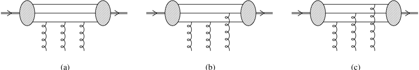
Figure 2.4: The three ways in which the odderon can couple to the proton in the lowest order.

Let us first consider one end of the odderon exchange, ie one half of the expression in the brackets in Equation 2.2.2. Three gluons can couple to the proton in the three ways displayed in Figure 2.4. Type (a) corresponds to the expression which contains the third-order term of one of the ${\bf V}_{i}^{a}$ and the $\delta_{\alpha\beta}$ of the two others (cf. Equation 2.15). Type (b) represents one in which there is the second-order term, first-order term and $\delta$ symbol of one ${\bf V}_{i}^{a}$, respectively. In type (c) the linear terms in $g$ of all three ${\bf V}_{i}^{a}$ appear. Since three gluons couple to each hadron, the sum of the orders of the contributing terms from the expansion of the three ${\bf V}_{i}^{a}$ has to be three.

The colour tensors differ according to the type of the coupling but are independent of the permutations, that is which gluon couples to which quark. They are calculated as follows:

$$\hbox{(a)}\quad C_{a}^{cc^{\prime}c^{\prime\prime}} = \epsilon_{\alpha\beta\gamma}\;(\tau^{c}\tau^{c^{\prime}}\tau^{c^{\prime\prime}})_{\alpha\alpha^{\prime}}\;\delta_{\beta\beta^{\prime}}\;\delta_{\gamma\gamma^{\prime}}\;\epsilon_{\alpha^{\prime}\beta^{\prime}\gamma^{\prime}}=\epsilon_{\alpha\beta\gamma}\;\epsilon_{\alpha^{\prime}\beta\gamma}\;(\tau^{c}\tau^{c^{\prime}}\tau^{c^{\prime\prime}})_{\alpha\alpha^{\prime}}$$

$$=2\,\delta_{\alpha\alpha^{\prime}}\,(\tau^{c}\tau^{c^{\prime}}\tau^{c^{\prime\prime}})_{\alpha\alpha^{\prime}}=2\,\hbox{Tr}(\tau^{c}\tau^{c^{\prime}}\tau^{c^{\prime\prime}})=\hbox{Tr}([\tau^{c},\tau^{c^{\prime}}]\tau^{c^{\prime\prime}}+\{\tau^{c},\tau^{c^{\prime}}\}\tau^{c^{\prime\prime}})$$

$$=\mathinner{1\over 2}if^{cc^{\prime}c^{\prime\prime}}+\mathinner{1\over 2}d^{cc^{\prime}c^{\prime\prime}}$$

$$\hbox{(b)}\quad C_{b}^{cc^{\prime}c^{\prime\prime}} = \epsilon_{\alpha\beta\gamma}\;(\tau^{c}\tau^{c^{\prime}})_{\alpha\alpha^{\prime}}\;\tau^{c^{\prime\prime}}_{\beta\beta^{\prime}}\;\delta_{\gamma\gamma^{\prime}}\;\epsilon_{\alpha^{\prime}\beta^{\prime}\gamma^{\prime}}=\epsilon_{\alpha\beta\gamma}\;\epsilon_{\alpha^{\prime}\beta^{\prime}\gamma}\;(\tau^{c}\tau^{c^{\prime}})_{\alpha\alpha^{\prime}}\;\tau^{c^{\prime\prime}}_{\beta\beta^{\prime}}$$

$$=(\delta_{\alpha\alpha^{\prime}}\;\delta_{\beta\beta^{\prime}}-\delta_{\alpha\beta^{\prime}}\;\delta_{\beta\alpha^{\prime}})\;(\tau^{c}\tau^{c^{\prime}})_{\alpha\alpha^{\prime}}\;\tau^{c}_{\beta\beta^{\prime}}=\hbox{Tr}(\tau^{c}\tau^{c^{\prime}})\;\hbox{Tr}(\tau^{c^{\prime\prime}})-\hbox{Tr}(\tau^{c}\tau^{c^{\prime}}\tau^{c^{\prime\prime}})$$

$$=-\hbox{Tr}(\tau^{c}\tau^{c^{\prime}}\tau^{c^{\prime\prime}})=-\mathinner{1\over 4}if^{cc^{\prime}c^{\prime\prime}}-\mathinner{1\over 4}d^{cc^{\prime}c^{\prime\prime}}$$

$$\hbox{(c)}\quad C_{c}^{cc^{\prime}c^{\prime\prime}} = \epsilon_{\alpha\beta\gamma}\;\tau^{c}_{\alpha\alpha^{\prime}}\;\tau^{c^{\prime}}_{\beta\beta^{\prime}}\;\tau^{c^{\prime\prime}}_{\gamma\gamma^{\prime}}\;\epsilon_{\alpha\beta\gamma}=\mathinner{1\over 2}d^{cc^{\prime}c^{\prime\prime}}\qquad\hbox{(numerically)}$$

As has been mentioned before, only the symmetric colour structure constants $d^{cc^{\prime}c^{\prime\prime}}$ are relevant for the odderon contribution because the structure in spinor space is antisymmetric. We obtain the following colour tensors for leading-order odderon exchange:

$$\hbox{(a)}\quad C_{a,\;{\rm odd}}^{cc^{\prime}c^{\prime\prime}} = \phantom{-}\mathinner{1\over 2}d^{cc^{\prime}c^{\prime\prime}}$$

$$\hbox{(b)}\quad C_{b,\;{\rm odd}}^{cc^{\prime}c^{\prime\prime}} = -\mathinner{1\over 4}d^{cc^{\prime}c^{\prime\prime}}$$ (2.17)

$$\hbox{(c)}\quad C_{c,\;{\rm odd}}^{cc^{\prime}c^{\prime\prime}} = \phantom{-}\mathinner{1\over 2}d^{cc^{\prime}c^{\prime\prime}}.$$

Having completed the investigation of the coupling types, we can now classify the Feynman graphs according to the types of the couplings at each hadron.

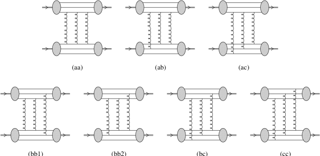
Figure 2.5: Seven exemplary Feynman graphs representing the seven graph types.

Combining three types of coupling at either end yields six possibilities, ignoring which type occurs at which hadron. However, two (b)-type couplings can be combined in two ways: The pair of gluons coupling to the same quark may or may not be the same at both ends. Hence we obtain seven types of Feynman graphs. One representative of each type is displayed in Figure 2.5. This classification was already used by Rüter in non-perturbative calculations [rueterphd].

The colour structure of the odderon gives an overall colour factor of $d^{cc^{\prime}c^{\prime\prime}}\,d^{cc^{\prime}c^{\prime\prime}}=\mathinner{40\over 3}$. In addition, the prefactors of the symmetric structure constants in Equation 2.2.4 contribute different factors to different graph types.

Another type-dependent factor comes from combinatorics: To facilitate our numerical calculations, we assume the gluons to be distinguishable. To compensate this overcounting, the result has to be divided by the number of permutations of gluons which couple to the same quarks. For instance, the contribution of the graphs of type (bb1) will be overcounted by a factor of two because for each graph an equivalent one will be calculated in which the two first gluons are exchanged (see Figure 2.5). By contrast, for type (bb2) the gluons are distinguished by which quarks they couple to and no overcounting occurs.

Table 2.1 shows the colour and combinatorial factors for each graph type. The total type-specific prefactor $C_{\rm type}$ is arbitrarily defined as one for graph type (aa). That means that an overall factor of $\mathinner{1\over 4}\mathinner{1\over 6}=\mathinner{1\over 24}$ has to be multiplied with $C_{\rm type}$ to get the right factor for a specific graph type. Also given in Table 2.1 is the number of graphs belonging to each type. They add up to the number of different Feynman graphs, 165.

A more rigorous derivation of the type-dependent prefactors is given in Section LABEL:sec:corrclass in Appendix LABEL:app:tofeyn. They arise from the coefficients in the expansion (2.15) and from summing up equivalent terms in the expansion of the six-gluon correlator (2.2.2).

  Type Colour factor Comb. factor $C$${}_{\rm type}$ # of graphs   (aa) $\mathinner{1\over 4}$ $\mathinner{1\over 6}$ $1\hbox to0.0pt{ (by definition)\hss}$ 9   (ab) $\hbox to0.0pt{\hss$-$}\mathinner{1\over 8}$ $\mathinner{1\over 2}$ $-\mathinner{3\over 2}$ 36   (ac) $\mathinner{1\over 4}$ $1$ $6$ 6   (bb1) $\mathinner{1\over 16}$ $\mathinner{1\over 2}$ $\mathinner{3\over 4}$ 36   (bb2) $\mathinner{1\over 16}$ $1$ $\mathinner{3\over 2}$ 36   (bc) $\hbox to0.0pt{\hss$-$}\mathinner{1\over 8}$ $1$ $-3$ 36   (cc) $\mathinner{1\over 4}$ $1$ $6$ 6

Table 2.1: Prefactors of the different graph types and number of Feynman graphs belonging to each type. See text for explanation.

2.2.5 The odderon-exchange scattering amplitude in the geometric model

We can now put everything together and write down the reduced scattering amplitude for odderon exchange between two protons described by our geometric model. Since the quarks have a relative position fixed by the rigid star shape, we can discard the six position variables ${\mathchoice{\hbox{\boldmath$\displaystyle x$}}{\hbox{\boldmath$\textstyle x$}}{\hbox{\boldmath$\scriptstyle x$}}{\hbox{\boldmath$\scriptscriptstyle x$}}\,_{i}^{a}}$ and use just two transverse-space vectors $\mathchoice{\hbox{\boldmath$\displaystyle R$}}{\hbox{\boldmath$\textstyle R$}}{\hbox{\boldmath$\scriptstyle R$}}{\hbox{\boldmath$\scriptscriptstyle R$}}_{i}$, $i=1,2$, which describe the radius and orientation of the star shape for each baryon.

The reduced scattering amplitude $J$ is defined as the scattering amplitude of two protons with fixed size and star angle, minus a total factor $2is$. It contains the overall factors we have computed so far: The colour factor $\mathinner{40\over 3}$, a factor $\mathinner{1\over 36}$ from Equation 2.2.2 and a conventional factor $\mathinner{1\over 24}$ extracted from the type-dependent prefactors.

$J$ sums up all Feynman graphs with the appropriate prefactors. It depends on the impact parameter $\textstyle b$ and the $\mathchoice{\hbox{\boldmath$\displaystyle R$}}{\hbox{\boldmath$\textstyle R$}}{\hbox{\boldmath$\scriptstyle R$}}{\hbox{\boldmath$\scriptscriptstyle R$}}_{i}$ which parametrise the size and orientation of each proton.

$$J(\mathchoice{\hbox{\boldmath$\displaystyle b$}}{\hbox{\boldmath$\textstyle b$}}{\hbox{\boldmath$\scriptstyle b$}}{\hbox{\boldmath$\scriptscriptstyle b$}},\mathchoice{\hbox{\boldmath$\displaystyle R$}}{\hbox{\boldmath$\textstyle R$}}{\hbox{\boldmath$\scriptstyle R$}}{\hbox{\boldmath$\scriptscriptstyle R$}}_{1},\mathchoice{\hbox{\boldmath$\displaystyle R$}}{\hbox{\boldmath$\textstyle R$}}{\hbox{\boldmath$\scriptstyle R$}}{\hbox{\boldmath$\scriptscriptstyle R$}}_{2})=\mathinner{1\over 36}\mathinner{40\over 3}\mathinner{1\over 24}g^{6}\sum_{\rm types}C_{\rm type}\sum_{\{a_{i}\}\,\{b_{i}\}}\hbox{\raise 2.0pt\hbox{$\chi$}}_{a_{1}b_{1}}\,\hbox{\raise 2.0pt\hbox{$\chi$}}_{a_{2}b_{2}}\,\hbox{\raise 2.0pt\hbox{$\chi$}}_{a_{3}b_{3}}$$ (2.18)

The second sum runs only over the sets of indices which are compatible with a specific graph type. The indices $a_{i}$ denote the quarks of the first proton the gluons couple to, the $b_{i}$ the quarks of the second proton. $\hbox{\raise 2.0pt\hbox{$\chi$}}_{ab}$ is the gluon propagator in transverse space:

$$\hbox{\raise 2.0pt\hbox{$\chi$}}_{ab}=\mathinner{i\over 2\pi}\,K_{0}(m\,|\mathchoice{\hbox{\boldmath$\displaystyle x$}}{\hbox{\boldmath$\textstyle x$}}{\hbox{\boldmath$\scriptstyle x$}}{\hbox{\boldmath$\scriptscriptstyle x$}}_{1}^{a}-\mathchoice{\hbox{\boldmath$\displaystyle x$}}{\hbox{\boldmath$\textstyle x$}}{\hbox{\boldmath$\scriptstyle x$}}{\hbox{\boldmath$\scriptscriptstyle x$}}_{2}^{b}|)\,.$$ (2.19)

It is derived in Appendix LABEL:sec:intlight. $m$ is a non-zero gluon mass which we have to introduce intermediately to compute $\chi$. In the gauge invariant expressions which arise after summing up all graphs it can be set to zero without causing problems.

The scattering amplitude is obtained by integrating over the reduced scattering amplitude with a wave function (2.1) for each proton. Since we want to obtain the odderon contribution as a function of the squared four momentum transfer $-t$, we have to Fourier transform it back into momentum space.

$$T(s,\mathchoice{\hbox{\boldmath$\displaystyle q$}}{\hbox{\boldmath$\textstyle q$}}{\hbox{\boldmath$\scriptstyle q$}}{\hbox{\boldmath$\scriptscriptstyle q$}})=2\,i\,s\int d^{2}\mathchoice{\hbox{\boldmath$\displaystyle b$}}{\hbox{\boldmath$\textstyle b$}}{\hbox{\boldmath$\scriptstyle b$}}{\hbox{\boldmath$\scriptscriptstyle b$}}\;e^{-i\,\mathchoice{\hbox{\boldmath$\displaystyle q$}}{\hbox{\boldmath$\textstyle q$}}{\hbox{\boldmath$\scriptstyle q$}}{\hbox{\boldmath$\scriptscriptstyle q$}}\mathchoice{\hbox{\boldmath$\displaystyle b$}}{\hbox{\boldmath$\textstyle b$}}{\hbox{\boldmath$\scriptstyle b$}}{\hbox{\boldmath$\scriptscriptstyle b$}}}\int d^{2}\mathchoice{\hbox{\boldmath$\displaystyle R$}}{\hbox{\boldmath$\textstyle R$}}{\hbox{\boldmath$\scriptstyle R$}}{\hbox{\boldmath$\scriptscriptstyle R$}}_{1}\int d^{2}\mathchoice{\hbox{\boldmath$\displaystyle R$}}{\hbox{\boldmath$\textstyle R$}}{\hbox{\boldmath$\scriptstyle R$}}{\hbox{\boldmath$\scriptscriptstyle R$}}_{2}\;|\psi(R_{1},S)|^{2}\;|\psi(R_{2},S)|^{2}\;J(\mathchoice{\hbox{\boldmath$\displaystyle b$}}{\hbox{\boldmath$\textstyle b$}}{\hbox{\boldmath$\scriptstyle b$}}{\hbox{\boldmath$\scriptscriptstyle b$}},\mathchoice{\hbox{\boldmath$\displaystyle R$}}{\hbox{\boldmath$\textstyle R$}}{\hbox{\boldmath$\scriptstyle R$}}{\hbox{\boldmath$\scriptscriptstyle R$}}_{1},\mathchoice{\hbox{\boldmath$\displaystyle R$}}{\hbox{\boldmath$\textstyle R$}}{\hbox{\boldmath$\scriptstyle R$}}{\hbox{\boldmath$\scriptscriptstyle R$}}_{2})$$ (2.20)

The polar angle in one of the three planar integrations is redundant since the forces between the hadrons depend only on their relative orientation. We can choose to measure the angles in the $\mathchoice{\hbox{\boldmath$\displaystyle R$}}{\hbox{\boldmath$\textstyle R$}}{\hbox{\boldmath$\scriptstyle R$}}{\hbox{\boldmath$\scriptscriptstyle R$}}_{1}$ and $\mathchoice{\hbox{\boldmath$\displaystyle R$}}{\hbox{\boldmath$\textstyle R$}}{\hbox{\boldmath$\scriptstyle R$}}{\hbox{\boldmath$\scriptscriptstyle R$}}_{2}$ planes relative to the vector $\textstyle b$. Then $J$ depends only on $b$ modulus. Hence we integrate out the angle in the $\textstyle b$ plane and get a factor $2\pi$ and a Bessel function $J_{0}$ instead of the exponential function from the Fourier transform. Using $|\mathchoice{\hbox{\boldmath$\displaystyle q$}}{\hbox{\boldmath$\textstyle q$}}{\hbox{\boldmath$\scriptstyle q$}}{\hbox{\boldmath$\scriptscriptstyle q$}}|=\sqrt{-t}$, the result reads:

$$T(s,t)=4\pi\,i\,s\int db\,b\int d^{2}\mathchoice{\hbox{\boldmath$\displaystyle R$}}{\hbox{\boldmath$\textstyle R$}}{\hbox{\boldmath$\scriptstyle R$}}{\hbox{\boldmath$\scriptscriptstyle R$}}_{1}\int d^{2}\mathchoice{\hbox{\boldmath$\displaystyle R$}}{\hbox{\boldmath$\textstyle R$}}{\hbox{\boldmath$\scriptstyle R$}}{\hbox{\boldmath$\scriptscriptstyle R$}}_{2}\;J_{0}(\sqrt{-t}\,b)\;|\psi(R_{1},S)|^{2}\;|\psi(R_{2},S)|^{2}\;J(b,\mathchoice{\hbox{\boldmath$\displaystyle R$}}{\hbox{\boldmath$\textstyle R$}}{\hbox{\boldmath$\scriptstyle R$}}{\hbox{\boldmath$\scriptscriptstyle R$}}_{1},\mathchoice{\hbox{\boldmath$\displaystyle R$}}{\hbox{\boldmath$\textstyle R$}}{\hbox{\boldmath$\scriptstyle R$}}{\hbox{\boldmath$\scriptscriptstyle R$}}_{2})\,.$$ (2.21)

The remaining integrals can only be evaluated numerically. We do this using the Vegas integration routine from Numerical Recipes, an adapting Monte-Carlo method. In most cases, 6 iterations of the algorithm with 5 000 000 evaluations of the integrand each were sufficient. For some values of the parameters, such as small angles in the star model, 8 iterations à 7 000 000 evaluations were used.

To determine the errors of the integration, it was executed several times with a different seed value for the random number generator on which the Monte-Carlo routine relies. The variation of the result proved a better indicator of the numerical errors than the built-in error estimation. The typical error in the scattering amplitude is 2 %, though it can be as much as 10 % for very small star angles or large $t$.

2.3 Calculation of the odderon scattering amplitude from impact factors in transverse momentum space

2.3.1 Introduction

Impact factors are expressions describing the coupling of a Reggeon being exchanged to the scattering particles. By that token, the calculations described in the previous section use impact factors in transverse position space based on the geometric model. Impact factors in momentum space are however far more common.

It can be shown that the scattering amplitude for a particular process factorises into two impact factors and a propagator. Hence, the odderon scattering amplitude is calculated by convoluting two odderon-proton impact factors with the propagators of the three gluons forming the odderon.

$$T(s,t)=2s\mathinner{40\over 3}\mathinner{1\over 3!}\mathinner{1\over(4\pi)^{4}}\int d^{2}\mathchoice{\hbox{\boldmath$\displaystyle\delta$}}{\hbox{\boldmath$\textstyle\delta$}}{\hbox{\boldmath$\scriptstyle\delta$}}{\hbox{\boldmath$\scriptscriptstyle\delta$}}_{1t}\,d^{2}\mathchoice{\hbox{\boldmath$\displaystyle\delta$}}{\hbox{\boldmath$\textstyle\delta$}}{\hbox{\boldmath$\scriptstyle\delta$}}{\hbox{\boldmath$\scriptscriptstyle\delta$}}_{2t}\,\Phi_{p}(\mathchoice{\hbox{\boldmath$\displaystyle\delta$}}{\hbox{\boldmath$\textstyle\delta$}}{\hbox{\boldmath$\scriptstyle\delta$}}{\hbox{\boldmath$\scriptscriptstyle\delta$}}_{1t},\mathchoice{\hbox{\boldmath$\displaystyle\delta$}}{\hbox{\boldmath$\textstyle\delta$}}{\hbox{\boldmath$\scriptstyle\delta$}}{\hbox{\boldmath$\scriptscriptstyle\delta$}}_{2t},\mathchoice{\hbox{\boldmath$\displaystyle\Delta$}}{\hbox{\boldmath$\textstyle\Delta$}}{\hbox{\boldmath$\scriptstyle\Delta$}}{\hbox{\boldmath$\scriptscriptstyle\Delta$}}_{t}-\mathchoice{\hbox{\boldmath$\displaystyle\delta$}}{\hbox{\boldmath$\textstyle\delta$}}{\hbox{\boldmath$\scriptstyle\delta$}}{\hbox{\boldmath$\scriptscriptstyle\delta$}}_{1t}-\mathchoice{\hbox{\boldmath$\displaystyle\delta$}}{\hbox{\boldmath$\textstyle\delta$}}{\hbox{\boldmath$\scriptstyle\delta$}}{\hbox{\boldmath$\scriptscriptstyle\delta$}}_{2t})^{2}\mathinner{1\over\mathchoice{\hbox{\boldmath$\displaystyle\delta$}}{\hbox{\boldmath$\textstyle\delta$}}{\hbox{\boldmath$\scriptstyle\delta$}}{\hbox{\boldmath$\scriptscriptstyle\delta$}}_{1t}^{2}\,\mathchoice{\hbox{\boldmath$\displaystyle\delta$}}{\hbox{\boldmath$\textstyle\delta$}}{\hbox{\boldmath$\scriptstyle\delta$}}{\hbox{\boldmath$\scriptscriptstyle\delta$}}_{2t}^{2}\,(\mathchoice{\hbox{\boldmath$\displaystyle\Delta$}}{\hbox{\boldmath$\textstyle\Delta$}}{\hbox{\boldmath$\scriptstyle\Delta$}}{\hbox{\boldmath$\scriptscriptstyle\Delta$}}_{t}-\mathchoice{\hbox{\boldmath$\displaystyle\delta$}}{\hbox{\boldmath$\textstyle\delta$}}{\hbox{\boldmath$\scriptstyle\delta$}}{\hbox{\boldmath$\scriptscriptstyle\delta$}}_{1t}-\mathchoice{\hbox{\boldmath$\displaystyle\delta$}}{\hbox{\boldmath$\textstyle\delta$}}{\hbox{\boldmath$\scriptstyle\delta$}}{\hbox{\boldmath$\scriptscriptstyle\delta$}}_{2t})^{2}}$$ (2.22)

$\mathchoice{\hbox{\boldmath$\displaystyle\delta$}}{\hbox{\boldmath$\textstyle\delta$}}{\hbox{\boldmath$\scriptstyle\delta$}}{\hbox{\boldmath$\scriptscriptstyle\delta$}}_{it},i=1,2,3$ are the transverse momenta of the gluons and $\mathchoice{\hbox{\boldmath$\displaystyle\Delta$}}{\hbox{\boldmath$\textstyle\Delta$}}{\hbox{\boldmath$\scriptstyle\Delta$}}{\hbox{\boldmath$\scriptscriptstyle\Delta$}}_{t}=\mathchoice{\hbox{\boldmath$\displaystyle\delta$}}{\hbox{\boldmath$\textstyle\delta$}}{\hbox{\boldmath$\scriptstyle\delta$}}{\hbox{\boldmath$\scriptscriptstyle\delta$}}_{1t}+\mathchoice{\hbox{\boldmath$\displaystyle\delta$}}{\hbox{\boldmath$\textstyle\delta$}}{\hbox{\boldmath$\scriptstyle\delta$}}{\hbox{\boldmath$\scriptscriptstyle\delta$}}_{2t}+\mathchoice{\hbox{\boldmath$\displaystyle\delta$}}{\hbox{\boldmath$\textstyle\delta$}}{\hbox{\boldmath$\scriptstyle\delta$}}{\hbox{\boldmath$\scriptscriptstyle\delta$}}_{3t}$ is the transverse momentum of the odderon. $40/3$ is the colour factor (equal to $d^{cc^{\prime}c^{\prime\prime}}\,d^{cc^{\prime}c^{\prime\prime}}$) and $1/3!$ the combinatorial factor reflecting the fact that the gluons are indistinguishable.

In the high energy limit $\mathchoice{\hbox{\boldmath$\displaystyle\Delta$}}{\hbox{\boldmath$\textstyle\Delta$}}{\hbox{\boldmath$\scriptstyle\Delta$}}{\hbox{\boldmath$\scriptscriptstyle\Delta$}}_{t}^{2}=-t$. This defines only the modulus of $\mathchoice{\hbox{\boldmath$\displaystyle\Delta$}}{\hbox{\boldmath$\textstyle\Delta$}}{\hbox{\boldmath$\scriptstyle\Delta$}}{\hbox{\boldmath$\scriptscriptstyle\Delta$}}_{t}$. Since the scattering amplitude depends only on $t$ and not on the vector $\mathchoice{\hbox{\boldmath$\displaystyle\Delta$}}{\hbox{\boldmath$\textstyle\Delta$}}{\hbox{\boldmath$\scriptstyle\Delta$}}{\hbox{\boldmath$\scriptscriptstyle\Delta$}}_{t}$, the integral has to be independent of its direction. This is true because both the propagators and the impact factors depend only on the relative orientation of the vectors $\mathchoice{\hbox{\boldmath$\displaystyle\delta$}}{\hbox{\boldmath$\textstyle\delta$}}{\hbox{\boldmath$\scriptstyle\delta$}}{\hbox{\boldmath$\scriptscriptstyle\delta$}}_{it}$. Since $\mathchoice{\hbox{\boldmath$\displaystyle\delta$}}{\hbox{\boldmath$\textstyle\delta$}}{\hbox{\boldmath$\scriptstyle\delta$}}{\hbox{\boldmath$\scriptscriptstyle\delta$}}_{1t}$ and $\mathchoice{\hbox{\boldmath$\displaystyle\delta$}}{\hbox{\boldmath$\textstyle\delta$}}{\hbox{\boldmath$\scriptstyle\delta$}}{\hbox{\boldmath$\scriptscriptstyle\delta$}}_{2t}$ are integrated over, the direction in which $\mathchoice{\hbox{\boldmath$\displaystyle\Delta$}}{\hbox{\boldmath$\textstyle\Delta$}}{\hbox{\boldmath$\scriptstyle\Delta$}}{\hbox{\boldmath$\scriptscriptstyle\Delta$}}_{t}$, and therefore $\mathchoice{\hbox{\boldmath$\displaystyle\delta$}}{\hbox{\boldmath$\textstyle\delta$}}{\hbox{\boldmath$\scriptstyle\delta$}}{\hbox{\boldmath$\scriptscriptstyle\delta$}}_{3t}$, points is irrelevant. Consequently in our calculations we assume that $\mathchoice{\hbox{\boldmath$\displaystyle\Delta$}}{\hbox{\boldmath$\textstyle\Delta$}}{\hbox{\boldmath$\scriptstyle\Delta$}}{\hbox{\boldmath$\scriptscriptstyle\Delta$}}_{t}$ points in one particular direction (rather than averaging over the polar angle in the $\mathchoice{\hbox{\boldmath$\displaystyle\Delta$}}{\hbox{\boldmath$\textstyle\Delta$}}{\hbox{\boldmath$\scriptstyle\Delta$}}{\hbox{\boldmath$\scriptscriptstyle\Delta$}}_{t}$ plane, for instance).

The two two-dimensional integrals in Equation 2.22 have to be evaluated numerically. We used the Vegas routine from Numerical Recipes with 5 iterations à 5 000 000 evaluations of the integrand. The errors in the scattering amplitude were smaller than 0.5 %.

2.3.2 The general form of the odderon-proton impact factor

It can be derived from the requirement of gauge invariance that the odderon-proton impact factor has to be of the following form:

$$\Phi_{p}=g^{3}\,[F(\mathchoice{\hbox{\boldmath$\displaystyle\Delta$}}{\hbox{\boldmath$\textstyle\Delta$}}{\hbox{\boldmath$\scriptstyle\Delta$}}{\hbox{\boldmath$\scriptscriptstyle\Delta$}}_{t},0,0)-\sum_{i=1}^{3}F(\mathchoice{\hbox{\boldmath$\displaystyle\delta$}}{\hbox{\boldmath$\textstyle\delta$}}{\hbox{\boldmath$\scriptstyle\delta$}}{\hbox{\boldmath$\scriptscriptstyle\delta$}}_{it},\mathchoice{\hbox{\boldmath$\displaystyle\Delta$}}{\hbox{\boldmath$\textstyle\Delta$}}{\hbox{\boldmath$\scriptstyle\Delta$}}{\hbox{\boldmath$\scriptscriptstyle\Delta$}}_{t}-\mathchoice{\hbox{\boldmath$\displaystyle\delta$}}{\hbox{\boldmath$\textstyle\delta$}}{\hbox{\boldmath$\scriptstyle\delta$}}{\hbox{\boldmath$\scriptscriptstyle\delta$}}_{it},0)+2F(\mathchoice{\hbox{\boldmath$\displaystyle\delta$}}{\hbox{\boldmath$\textstyle\delta$}}{\hbox{\boldmath$\scriptstyle\delta$}}{\hbox{\boldmath$\scriptscriptstyle\delta$}}_{1t},\mathchoice{\hbox{\boldmath$\displaystyle\delta$}}{\hbox{\boldmath$\textstyle\delta$}}{\hbox{\boldmath$\scriptstyle\delta$}}{\hbox{\boldmath$\scriptscriptstyle\delta$}}_{2t},\mathchoice{\hbox{\boldmath$\displaystyle\delta$}}{\hbox{\boldmath$\textstyle\delta$}}{\hbox{\boldmath$\scriptstyle\delta$}}{\hbox{\boldmath$\scriptscriptstyle\delta$}}_{3t})]\,.$$ (2.23)

The first expression in the brackets represents the diagram (a) in Figure 2.4, the second diagram (b), and the third corresponds to diagram (c). (Due to gauge invariance, all diagrams have to be there.) $F(\mathchoice{\hbox{\boldmath$\displaystyle\delta$}}{\hbox{\boldmath$\textstyle\delta$}}{\hbox{\boldmath$\scriptstyle\delta$}}{\hbox{\boldmath$\scriptscriptstyle\delta$}}_{1t},\mathchoice{\hbox{\boldmath$\displaystyle\delta$}}{\hbox{\boldmath$\textstyle\delta$}}{\hbox{\boldmath$\scriptstyle\delta$}}{\hbox{\boldmath$\scriptscriptstyle\delta$}}_{2t},\mathchoice{\hbox{\boldmath$\displaystyle\delta$}}{\hbox{\boldmath$\textstyle\delta$}}{\hbox{\boldmath$\scriptstyle\delta$}}{\hbox{\boldmath$\scriptscriptstyle\delta$}}_{3t})$ is the proton form factor which can be chosen in different ways.

The form factor has to be constructed so that the impact factor vanishes when one of the $\mathchoice{\hbox{\boldmath$\displaystyle\delta$}}{\hbox{\boldmath$\textstyle\delta$}}{\hbox{\boldmath$\scriptstyle\delta$}}{\hbox{\boldmath$\scriptscriptstyle\delta$}}_{it}$ is zero. This is required by gauge invariance and has the additional benefit that the integrand in Equation 2.22 is analytic.

2.3.3 The form factor of Levin and Ryskin

A paper on proton-proton scattering by Levin and Ryskin [lev] uses a Gaussian form factor for the proton. It is constructed in such a way that it gives a significant contribution only when all the gluon momenta are small.

$$F(\mathchoice{\hbox{\boldmath$\displaystyle\delta$}}{\hbox{\boldmath$\textstyle\delta$}}{\hbox{\boldmath$\scriptstyle\delta$}}{\hbox{\boldmath$\scriptscriptstyle\delta$}}_{1t},\mathchoice{\hbox{\boldmath$\displaystyle\delta$}}{\hbox{\boldmath$\textstyle\delta$}}{\hbox{\boldmath$\scriptstyle\delta$}}{\hbox{\boldmath$\scriptscriptstyle\delta$}}_{2t},\mathchoice{\hbox{\boldmath$\displaystyle\delta$}}{\hbox{\boldmath$\textstyle\delta$}}{\hbox{\boldmath$\scriptstyle\delta$}}{\hbox{\boldmath$\scriptscriptstyle\delta$}}_{3t})=\exp\left(-R_{p}^{2}\,\left(\mathchoice{\hbox{\boldmath$\displaystyle\delta$}}{\hbox{\boldmath$\textstyle\delta$}}{\hbox{\boldmath$\scriptstyle\delta$}}{\hbox{\boldmath$\scriptscriptstyle\delta$}}_{1t}^{2}+\mathchoice{\hbox{\boldmath$\displaystyle\delta$}}{\hbox{\boldmath$\textstyle\delta$}}{\hbox{\boldmath$\scriptstyle\delta$}}{\hbox{\boldmath$\scriptscriptstyle\delta$}}_{2t}^{2}+\mathchoice{\hbox{\boldmath$\displaystyle\delta$}}{\hbox{\boldmath$\textstyle\delta$}}{\hbox{\boldmath$\scriptstyle\delta$}}{\hbox{\boldmath$\scriptscriptstyle\delta$}}_{3t}^{2}\right)\right)$$ (2.24)

There is some confusion about the proton radius $R_{p}$ since it is given in the paper [lev] as “$R_{p}^{2}=2.75$ GeV${}^{2}$”. The more reasonable value of $R_{p}=0.32723$ fm is obtained when assuming the wrong sign to be in the exponent of the unit GeV.

2.3.4 The form factor of Kwieciński et al.

In 1997, Kwieciński et al. published calculations of the odderon exchange in the photo- and electroproduction of the $\eta_{c}$ meson [kwie_impac], based on earlier work by Fukugita and Kwieciński [fk]. To that end, they compute odderon-photon and odderon-proton impact factors. For us only the odderon-proton impact factor is of interest. It is constructed according to Equation 2.23 from the following form factor:

$$F(\mathchoice{\hbox{\boldmath$\displaystyle\delta$}}{\hbox{\boldmath$\textstyle\delta$}}{\hbox{\boldmath$\scriptstyle\delta$}}{\hbox{\boldmath$\scriptscriptstyle\delta$}}_{1t},\mathchoice{\hbox{\boldmath$\displaystyle\delta$}}{\hbox{\boldmath$\textstyle\delta$}}{\hbox{\boldmath$\scriptstyle\delta$}}{\hbox{\boldmath$\scriptscriptstyle\delta$}}_{2t},\mathchoice{\hbox{\boldmath$\displaystyle\delta$}}{\hbox{\boldmath$\textstyle\delta$}}{\hbox{\boldmath$\scriptstyle\delta$}}{\hbox{\boldmath$\scriptscriptstyle\delta$}}_{3t})=\mathinner{A^{2}\over A^{2}+\mathinner{1\over 2}[(\mathchoice{\hbox{\boldmath$\displaystyle\delta$}}{\hbox{\boldmath$\textstyle\delta$}}{\hbox{\boldmath$\scriptstyle\delta$}}{\hbox{\boldmath$\scriptscriptstyle\delta$}}_{1t}-\mathchoice{\hbox{\boldmath$\displaystyle\delta$}}{\hbox{\boldmath$\textstyle\delta$}}{\hbox{\boldmath$\scriptstyle\delta$}}{\hbox{\boldmath$\scriptscriptstyle\delta$}}_{2t})^{2}+(\mathchoice{\hbox{\boldmath$\displaystyle\delta$}}{\hbox{\boldmath$\textstyle\delta$}}{\hbox{\boldmath$\scriptstyle\delta$}}{\hbox{\boldmath$\scriptscriptstyle\delta$}}_{2t}-\mathchoice{\hbox{\boldmath$\displaystyle\delta$}}{\hbox{\boldmath$\textstyle\delta$}}{\hbox{\boldmath$\scriptstyle\delta$}}{\hbox{\boldmath$\scriptscriptstyle\delta$}}_{3t})^{2}+(\mathchoice{\hbox{\boldmath$\displaystyle\delta$}}{\hbox{\boldmath$\textstyle\delta$}}{\hbox{\boldmath$\scriptstyle\delta$}}{\hbox{\boldmath$\scriptscriptstyle\delta$}}_{3t}-\mathchoice{\hbox{\boldmath$\displaystyle\delta$}}{\hbox{\boldmath$\textstyle\delta$}}{\hbox{\boldmath$\scriptstyle\delta$}}{\hbox{\boldmath$\scriptscriptstyle\delta$}}_{1t})^{2}]}.$$ (2.25)

Its width is proportional to $A$ which was chosen by the authors to be half the rho mass, 384 MeV. Unlike the form factor of Levin and Ryskin, it can still give a significant contribution when the gluon momenta are large. This is the case when they are large but close to each other, ie when the gluons move in the same direction.

2.4 The Donnachie-Landshoff fit: A complete set of contributions to elastic $pp$ and $p\bar{p}$ scattering

In order to fit experimental data of proton-proton scattering, one has to take into account other contributions besides the odderon. We decided to obtain those from the phenomenological fit by A. Donnachie and P. Landshoff published in 1984 [dlfit]. It is well-known for reproducing the dip in the differential cross section in proton-proton scattering. Remarkably, the same parameter values fit the data for any centre-of-mass energy, and the wandering of the dip with changing $s$ results automatically.

We use the Donnachie-Landshoff fit as a phenomenological input to our calculations. Since it depends only weakly on $\alpha_{s}$, in most cases we leave $\alpha_{s}$ constant at 0.3, the value used in the original work. Whenever it is changed, this will be noted in the results in chapters 3 and 4.

Donnachie and Landshoff take into account a number of contributions to the elastic proton-proton scattering amplitude. They will be described briefly in the following sections. For details see [dlfit].

2.4.1 All contributions of the DL fit

The pomeron

The pomeron is described in the framework of Regge theory (see section 1.4.2). Donnachie and Landshoff’s pomeron has intercept $\alpha_{\mathchoice{\hbox{$\displaystyle\mathbb{P}$}}{\hbox{$\textstyle\mathbb{P}$}}{\hbox{$\scriptstyle\mathbb{P}$}}{\hbox{$\scriptscriptstyle\mathbb{P}$}}}(0)=1.08$ and slope $\alpha^{\prime}_{\mathchoice{\hbox{$\displaystyle\mathbb{P}$}}{\hbox{$\textstyle\mathbb{P}$}}{\hbox{$\scriptstyle\mathbb{P}$}}{\hbox{$\scriptscriptstyle\mathbb{P}$}}}=0.25\hbox{ GeV}^{-2}$.

To describe the pomeron-proton coupling, Donnachie and Landshoff use a proton form factor of the following form:

$$F_{1}(t)=\mathinner{4m^{2}-2.79t\over 4m^{2}-t}\mathinner{1\over(1-t/0.71)^{2}}\,.$$

The complete expression for the scattering amplitude is as follows. (It differs by a factor of two from [dlfit] since our definition of the scattering amplitude is different by that factor, cf. Equation 1.2.)

$$T_{\mathchoice{\hbox{$\displaystyle\mathbb{P}$}}{\hbox{$\textstyle\mathbb{P}$}}{\hbox{$\scriptstyle\mathbb{P}$}}{\hbox{$\scriptscriptstyle\mathbb{P}$}}}(s,t)=2i\,s\,\left(3\,\beta\,F_{1}(t)\right)^{2}\,\left(\mathinner{-i\,s\over m^{2}}\right)^{\alpha_{\mathchoice{\hbox{$\displaystyle\mathbb{P}$}}{\hbox{$\textstyle\mathbb{P}$}}{\hbox{$\scriptstyle\mathbb{P}$}}{\hbox{$\scriptscriptstyle\mathbb{P}$}}}(t)-1}$$

Since the pomeron is even under charge conjugation, it contributes equally to proton-proton and proton-antiproton scattering.

The Reggeon contribution

The Reggeon contribution combines the effects of four different particle exchanges: $\rho$ and $\omega$ (which are odd under charge conjugation), and $f$ and $a_{2}$ (which are even). All four particles lie on the Regge trajectory with intercept 0.44 and slope 0.93 GeV${}^{-2}$. In addition to the form factor and constant factors of the pomeron contribution there is a complex factor. To account for the fact that two of the described particles are odd under charge conjugation, it has to be replaced by its complex conjugate when describing proton-antiproton scattering.

Three-particle contributions

Three different three-particle exchanges are taken into account: triple-gluon exchange, triple-pomeron exchange and simultaneous exchange of two gluons and one pomeron. For all of them, the scattering amplitude has the following form:

$$T_{3}(s,t)=2s\mathinner{K\over\hbox{-}t+t_{0}}\int dx_{1}dx_{2}dx_{3}\,\delta(1\hbox{-}x_{1}\hbox{-}x_{2}\hbox{-}x_{3})\,(x_{1}x_{2}x_{3})^{2}V(x_{1},x_{2},x_{3})^{4}\,D(s_{1},t_{1})D(s_{2},t_{2})D(s_{3},t_{3})\,.$$

$x_{i}$ are the transverse momentum fractions of the three particles, and $s_{i}=x_{i}^{2}s$ and $t_{i}=x_{i}^{2}t$. $V(x_{1},x_{2},x_{3})=Ax_{1}x_{2}x_{3}$ is the vertex function (wave function), and the $D(s,t)$ are the propagators of the particles. The constant $A$ in the vertex function must be fitted so that the triple-gluon contribution approaches an asymptotic power law for the differential cross-section: $d\sigma/dt=0.09\hbox{ mb GeV}^{14}\,\cdot\,t^{-8}$. (See [dlt-8] for more on the power law.)

Figure 2.6: The cut-off gluon propagator used by Donnachie and Landshoff.

The gluon propagator is $\alpha_{s}/t$ for large $|t|$. For small $|t|$ it is cut off with a parabola through the origin (see Figure 2.6). It is independent of $s$. The following ansatz is made for the parabola:

$$D_{g}(t)=\lambda t(t+\tau)\qquad\hbox{for $-t<t_{1}$}\,.$$

$\lambda$ and $\tau$ are fixed by requiring continuity of $D_{g}(t)$ and its derivative. This gives $\lambda=2/t_{1}^{3}$ and $\tau=-\mathinner{3\over 2}\;t_{1}$.

The pomeron propagator is derived from its Regge trajectory:

$$D_{\mathchoice{\hbox{$\displaystyle\mathbb{P}$}}{\hbox{$\textstyle\mathbb{P}$}}{\hbox{$\scriptstyle\mathbb{P}$}}{\hbox{$\scriptscriptstyle\mathbb{P}$}}}(s,t)=\mathinner{\beta^{2}\over 4\pi}i\left(\mathinner{-i\,s\over m^{2}}\right)^{\alpha_{\mathchoice{\hbox{$\displaystyle\mathbb{P}$}}{\hbox{$\textstyle\mathbb{P}$}}{\hbox{$\scriptstyle\mathbb{P}$}}{\hbox{$\scriptscriptstyle\mathbb{P}$}}}(t)-1}\,.$$

Depending on what particles are exchanged, three gluon propagators, three pomeron propagators or one pomeron and two gluon propagators must be used. The triple-gluon exchange contribution is odd under charge conjugation, the other two contributions are even.

Even though the gluon propagator contains the coupling constant, the Donnachie-Landshoff fit is nearly independent of it. This is because the constant $A$ which appears alongside the coupling constant is determined by fitting the $ggg$ contribution to the asymptotic power law. Therefore any change in the coupling constant in the triple gluon contribution is compensated by a change in $A$. The other three-particle exchanges depend on $A$ and hence change when $A$ varies as a result of a change in $\alpha_{s}$. However, this has little effect since they are rather less important.

Reggeon-pomeron and double pomeron exchange

To obtain an expression for simultaneous exchange of a Reggeons and a pomeron, their trajectories are combined in the following way: $\alpha_{{\mathchoice{\hbox{$\displaystyle\mathbb{R}$}}{\hbox{$\textstyle\mathbb{R}$}}{\hbox{$\scriptstyle\mathbb{R}$}}{\hbox{$\scriptscriptstyle\mathbb{R}$}}}{\mathchoice{\hbox{$\displaystyle\mathbb{P}$}}{\hbox{$\textstyle\mathbb{P}$}}{\hbox{$\scriptstyle\mathbb{P}$}}{\hbox{$\scriptscriptstyle\mathbb{P}$}}}}(t)=\alpha_{\mathchoice{\hbox{$\displaystyle\mathbb{R}$}}{\hbox{$\textstyle\mathbb{R}$}}{\hbox{$\scriptstyle\mathbb{R}$}}{\hbox{$\scriptscriptstyle\mathbb{R}$}}}(0)+\alpha_{\mathchoice{\hbox{$\displaystyle\mathbb{P}$}}{\hbox{$\textstyle\mathbb{P}$}}{\hbox{$\scriptstyle\mathbb{P}$}}{\hbox{$\scriptscriptstyle\mathbb{P}$}}}(0)-1+\mathinner{\alpha_{\mathchoice{\hbox{$\displaystyle\mathbb{R}$}}{\hbox{$\textstyle\mathbb{R}$}}{\hbox{$\scriptstyle\mathbb{R}$}}{\hbox{$\scriptscriptstyle\mathbb{R}$}}}^{\prime}\alpha_{\mathchoice{\hbox{$\displaystyle\mathbb{P}$}}{\hbox{$\textstyle\mathbb{P}$}}{\hbox{$\scriptstyle\mathbb{P}$}}{\hbox{$\scriptscriptstyle\mathbb{P}$}}}^{\prime}\over\alpha_{\mathchoice{\hbox{$\displaystyle\mathbb{R}$}}{\hbox{$\textstyle\mathbb{R}$}}{\hbox{$\scriptstyle\mathbb{R}$}}{\hbox{$\scriptscriptstyle\mathbb{R}$}}}^{\prime}+\alpha_{\mathchoice{\hbox{$\displaystyle\mathbb{P}$}}{\hbox{$\textstyle\mathbb{P}$}}{\hbox{$\scriptstyle\mathbb{P}$}}{\hbox{$\scriptscriptstyle\mathbb{P}$}}}^{\prime}}t$. In the case of double pomeron exchange, the analogous formula is $\alpha_{{\mathchoice{\hbox{$\displaystyle\mathbb{P}$}}{\hbox{$\textstyle\mathbb{P}$}}{\hbox{$\scriptstyle\mathbb{P}$}}{\hbox{$\scriptscriptstyle\mathbb{P}$}}}{\mathchoice{\hbox{$\displaystyle\mathbb{P}$}}{\hbox{$\textstyle\mathbb{P}$}}{\hbox{$\scriptstyle\mathbb{P}$}}{\hbox{$\scriptscriptstyle\mathbb{P}$}}}}(t)=2\alpha_{\mathchoice{\hbox{$\displaystyle\mathbb{P}$}}{\hbox{$\textstyle\mathbb{P}$}}{\hbox{$\scriptstyle\mathbb{P}$}}{\hbox{$\scriptscriptstyle\mathbb{P}$}}}(0)-1+\mathinner{1\over 2}\alpha_{\mathchoice{\hbox{$\displaystyle\mathbb{P}$}}{\hbox{$\textstyle\mathbb{P}$}}{\hbox{$\scriptstyle\mathbb{P}$}}{\hbox{$\scriptscriptstyle\mathbb{P}$}}}^{\prime}t$. The scattering amplitude is calculated from the trajectories of double pomeron and Reggeon-pomeron exchange in the following way:

$$T_{{\mathchoice{\hbox{$\displaystyle\mathbb{P}$}}{\hbox{$\textstyle\mathbb{P}$}}{\hbox{$\scriptstyle\mathbb{P}$}}{\hbox{$\scriptscriptstyle\mathbb{P}$}}}{\mathchoice{\hbox{$\displaystyle\mathbb{P}$}}{\hbox{$\textstyle\mathbb{P}$}}{\hbox{$\scriptstyle\mathbb{P}$}}{\hbox{$\scriptscriptstyle\mathbb{P}$}}}}(s,t) = \mathinner{-2iD\beta^{4}F_{1}(t)\over\log(s/m^{2})}\,\left(\mathinner{-i\,s\over m^{2}}\right)^{\alpha_{{\mathchoice{\hbox{$\displaystyle\mathbb{P}$}}{\hbox{$\textstyle\mathbb{P}$}}{\hbox{$\scriptstyle\mathbb{P}$}}{\hbox{$\scriptscriptstyle\mathbb{P}$}}}{\mathchoice{\hbox{$\displaystyle\mathbb{P}$}}{\hbox{$\textstyle\mathbb{P}$}}{\hbox{$\scriptstyle\mathbb{P}$}}{\hbox{$\scriptscriptstyle\mathbb{P}$}}}}(t)-1}$$

$$T_{{\mathchoice{\hbox{$\displaystyle\mathbb{R}$}}{\hbox{$\textstyle\mathbb{R}$}}{\hbox{$\scriptstyle\mathbb{R}$}}{\hbox{$\scriptscriptstyle\mathbb{R}$}}}{\mathchoice{\hbox{$\displaystyle\mathbb{P}$}}{\hbox{$\textstyle\mathbb{P}$}}{\hbox{$\scriptstyle\mathbb{P}$}}{\hbox{$\scriptscriptstyle\mathbb{P}$}}}}(s,t) = \mathinner{-4iD\beta^{4}F_{1}(t)\over\log(s/m^{2})}\,(A+iB)\,\left(\mathinner{-i\,s\over m^{2}}\right)^{\alpha_{{\mathchoice{\hbox{$\displaystyle\mathbb{R}$}}{\hbox{$\textstyle\mathbb{R}$}}{\hbox{$\scriptstyle\mathbb{R}$}}{\hbox{$\scriptscriptstyle\mathbb{R}$}}}{\mathchoice{\hbox{$\displaystyle\mathbb{P}$}}{\hbox{$\textstyle\mathbb{P}$}}{\hbox{$\scriptstyle\mathbb{P}$}}{\hbox{$\scriptscriptstyle\mathbb{P}$}}}}(t)-1}\,,$$

where $(A+iB)$ is the same complex prefactor which occurs in the Reggeon contribution.

How to produce the dip

The dip in proton-proton scattering results from a three-way interference between the following contributions: pomeron exchange, double pomeron exchange and triple gluon (odderon) exchange. The constant $D$ in the double pomeron contribution is adjusted so that the imaginary part of pomeron and double pomeron exchange cancel at the dip. Since both are nearly imaginary in the vicinity of the dip, only a small real part remains. The odderon contribution further diminishes the real part, which gives the dip.

The other contributions are much smaller in size. They serve for fine-tuning the depth and position of the dip.

2.4.2 The odderon contribution in the Donnachie-Landshoff fit

This section will take a closer look at the triple gluon exchange contribution of the Donnachie-Landshoff fit. It evaluates a single Feynman diagram displayed in Figure 2.7. This diagram corresponds to two type (c) couplings according to the classification in Section 2.2.4.

Figure 2.7: The diagram corresponding to Donnachie and Landshoff’s triple gluon contribution.

This has two implications. First, since only a single diagram is included, the expression is not gauge invariant. This is the reason why the gluon propagator has to be cut off to prevent infra-red divergences.

The second implication of choosing this specific diagram is its colour structure: It is the purely symmetric $\mathinner{1\over 2}d^{cc^{\prime}c^{\prime\prime}}$ (see Equation 2.2.4). Taking the antisymmetric structure in spinor space into account, it follows that the contribution is odd under charge conjugation. Hence it is an odderon even though the authors do not call it that.

A final remark concerning the triple gluon exchange contribution has to be made and will be of great help to anybody reproducing the Donnachie-Landshoff fit. There appears to be a misprint in the paper describing the fit [dlfit]. The gluon propagator cutoff $t_{1}$ and the scale $t_{0}$ which corresponds to the proton radius are given as “$t_{0}=t_{1}=300\;\hbox{MeV}^{2}$”. This value results in a $ggg$ contribution which is far too large, dominating the differential cross section for all $t$. In a later paper about a slightly modified fit [dlfitnew] (described below), the authors mention $t_{1}$ as having previously had the value 0.3 GeV${}^{2}$. Indeed choosing this value produces a good fit. Therefore, we use this parameter value for both $t_{0}$ and $t_{1}$.

2.4.3 The improved fit of 1986

While the DL fit is fairly good at ISR energies, it does not fit higher-energy collider data. In Section 4.3.1, this will be shown in detail and attempts to improve it will be presented.

This state of affairs was already remarked upon by Gauron, Leader and Nicolescu in 1985 [gnldlcrit]. In response to their criticism, Donnachie and Landshoff published an improved version of their fit which they claim both extends to collider energies and shows some improvement at ISR energies [dlfitnew]. While it seems quite plausible that the Regge-plus-dynamics description of Donnachie and Landshoff should be able to accommodate high-energy data, I have not been able to reproduce the improved fit.

In all probability the authors changed some aspects of the fit without mentioning it in [dlfitnew]. It is unfortunate but was to be expected that today they cannot remember any details any more. I followed the prescription given in [dlfitnew] but start to disagree with the paper at the point where according to the authors the double-pomeron contribution has to be increased significantly. In my reproduction of the fit, it in fact has to be made smaller (though very slightly) to make the imaginary part of the total amplitude vanish as prescribed in the paper.

Chapter 3 The results for $pp$ scattering

3.1 Experimental data

Since we use the Donnachie-Landshoff fit as a framework for different odderon contributions, we use data for proton-proton scattering in the range where we know the fit is valid. This is the case for the energy range investigated by experiments at the Intersecting Storage Rings (ISR) at CERN. Data from the ISR were also used by Donnachie and Landshoff themselves.

The differential elastic proton-proton cross section has been measured by a number of collaborations at the ISR. Measurements have been made at the centre-of-mass energies 23.5 GeV, 30.7 GeV, 44.7 GeV, 52.8 GeV and 62.5 GeV. All the data we used were obtained from the Durham/RAL database [durdata]. For all energies except 52.8 GeV, we used the data sets as collected by Amaldi and Schubert [ama]. Amaldi and Schubert did not do any measurements themselves for this paper; rather, they collected all ISR data and applied a normalisation to data which were not yet normalised. The data in the $t$ range relevant for us were measured by Nagy and collaborators [nagy] and Böhm and collaborators [bohm]. The latter data were normalised by Amaldi and Schubert.

For the centre-of-mass energy 52.8 GeV, we used the data published by Nagy et al. [nagy]. The data given by Amaldi and Schubert for that energy do not extend to the $t$ region of interest to us. We complement the data from [nagy] with data measured by Breakstone and collaborators [break] even though they were measured at 53 GeV centre-of-mass energy. It can be seen in the plots that they do not always coincide, suggesting some experimental uncertainty. The $s$ dependence of the differential cross section is too small to explain the discrepancy. We decided against using the data from Erhan and collaborators [erhan] since they were available only for relatively few values of $t$ and tended to coincide with the Breakstone data.

3.2 The fit of Donnachie and Landshoff

3.2.1 Fixed coupling

Initially we had some problems reproducing the Donnachie-Landshoff fit. This was due to a misprint in [dlfit] (see Section 2.4.2). The constant $t_{0}$ in the expression for the three-particle exchanges (which gives the scale corresponding to the proton radius) and the the gluon propagator cutoff $t_{1}$ is 0.3 GeV${}^{2}$ rather than the value given in the paper. The original fit reproduced with these parameter values is displayed in Figure 3.1.

Figure 3.1: The original Donnachie-Landshoff fit with constant coupling. Data for five centre-of-mass energies are plotted simultaneously. The scale on the left applies to the lowest curve only. Successive curves are shifted upwards by a factor of 100. The points with error bars are experimental data. See Section 3.1 for their sources.

3.2.2 Different cutoffs of the gluon propagator

To show that the Donnachie-Landshoff fit is independent of the precise nature of the gluon propagator cutoff, alternative ways of cutting off were tried. The two possibilities were a flat and a linearly rising propagator for small $|t|$, see Figure 3.2.

Changes in the integral over the propagator can be compensated by changes in the constants $t_{1}$ and $A$. The resulting curves are not shown here since they are practically identical to the original fit shown in Figure 3.1.

Figure 3.2: The two alternative ways of cutting off the gluon propagator.

3.2.3 Running coupling

In a leading-order calculation, the coupling constant is just that, a constant. However, it is known that in reality the strong coupling constant depends on the scale. It is possible with limited extra effort to take this into account and see how it influences our results. We replaced the strong coupling constant with the following expression for the running coupling:

$$\alpha_{s}(t)=\mathinner{4\pi\over\left(\mathinner{11\over 3}N_{c}-\mathinner{2\over 3}N_{f}\right)\log\left(\mathinner{|t|\over\Lambda_{\rm QCD}^{2}}+6\right)}\,.$$ (3.1)

This is the one-loop expression for the running of $\alpha_{s}$ modified to account for non-perturbative effects. The constant 6 was added in the logarithm to avoid the divergence of the perturbative running coupling, which is called “freezing” of the coupling constant. This specific way of freezing $\alpha_{s}$ has been used before by Ewerz [ewmodalpha]. The number of colours $N_{c}$ is 3, and we have set the number of flavours $N_{f}$ also to 3. $\Lambda_{\rm QCD}$ was chosen to be 250 MeV.

The fit with the running coupling is as good as the original fit, see Figure 3.3.

Figure 3.3: The Donnachie-Landshoff fit with running coupling.

Figure 3.4: The fit with the odderon computed in the quark-diquark model, with constant coupling.

3.3 The fit with the geometric model odderon

3.3.1 Fixed coupling

The main aim of our calculations in the quark-diquark model was to determine the diquark size. For that purpose we substituted the diquark model odderon amplitude for the triple-gluon contribution in the Donnachie-Landshoff fit. The coupling constant of the DL contributions was left at 0.3 since that is what its authors chose. (In fact only the ${\mathchoice{\hbox{$\displaystyle\mathbb{P}$}}{\hbox{$\textstyle\mathbb{P}$}}{\hbox{$\scriptstyle\mathbb{P}$}}{\hbox{$\scriptscriptstyle\mathbb{P}$}}}gg$ and the $\textstyle\mathbb{P}$$\textstyle\mathbb{P}$$\textstyle\mathbb{P}$ contributions depend on $\alpha_{s}$.) We use the DL fit as a framework in which several odderon contributions are substituted for the original one. For our geometric odderon contribution, we chose the coupling constant 0.4 since it is in the middle of the range $0.3\ldots 0.5$ common in the literature at the scale given by $-t$ at the dip. See Section 3.3.2 for a discussion of other values for the coupling constant.

The diquark size (respectively the angle in Figure 2.2) was adjusted to give the best fit for a range of centre-of-mass energies. The result can be seen in Figure 3.4. The optimal angle is 0.14$\,\pi$, or approximately 25 degrees (in transverse space). This corresponds to a diquark size in transverse space of 0.22 fm according to Formula 2.2. This diquark size justifies a practice common in non-perturbative calculations. Since soft gluons cannot resolve a diquark as small as 0.3 fm, it is legitimate to treat the proton as a colour dipole, as in [dfk, bergnacht, ssmsv3], for example.

Choosing the correct angle is vital for obtaining a good fit. Figure 3.5 shows that the fit gets considerably worse when the angle is maladjusted. The dependence of the odderon contribution on the diquark size will be analysed in greater detail in the next section.

Figure 3.5: The fit with the quark-diquark model odderon for different star angles. The drawn-out curve is the best fit, 0.14$\,\pi$. The centre-of-mass energy is 44.7 GeV.

3.3.2 The value of the coupling constant and the significance of the fit

The quality of the fit depends strongly on the size of the odderon contribution in the dip region. That is why we were able to determine the diquark size (on which the size of the odderon depends) from the fit of $d\sigma/dt$. However, the odderon contribution also depends strongly on the coupling constant: it is proportional to $\alpha_{s}^{6}$. Therefore the optimal value for the diquark size depends on the choice of the coupling constant (or the choice of $\Lambda_{\hbox{\scriptsize QCD}}$ if $\alpha_{s}$ is running).

The difficulty here lies in the fact that in a leading-order calculation the value of the coupling can only be estimated. Determining the scale relevant for the coupling and the “true” value of the coupling constant requires higher-order calculations. We have therefore determined the optimal diquark size for several values of $\alpha_{s}$.

  $\alpha_{s}$ star angle diquark size [fm]   0.3      $0.22\,\pi$ 0.34   0.4      $0.14\,\pi$ 0.22   0.5      $0.095\,\pi$ 0.15

Table 3.1: Optimal diquark size for the odderon in the geometric model for different coupling constants.

The values for $\alpha_{s}$ which are common in the literature at this scale in the momentum transfer lie in the range from 0.3 to 0.5. Table 3.1 shows how the optimal diquark size for several the coupling constants. Since the scattering amplitude rises both with the diquark size and with $\alpha_{s}$, the diquark size has to be larger for a smaller coupling constant. All resulting sizes for the diquark cluster in the proton are $\lesssim 0.35\;$fm, supporting the assumption of a reasonably small diquark unless the coupling constant is smaller than 0.3.

The other extreme, a rotationally symmetric “Mercedes star” proton, can be excluded with some confidence. This would imply an unrealistically small coupling constant of 0.17.

Figure 3.6: The dependence of the quark-diquark model odderon amplitude on the diquark size. The error bars reflect the numerical errors of up to 10%. The three points for each value of the diquark size correspond to three different transverse momentum transfers. The square of the momentum transfer $-t$ is 0.6 GeV${}^{2}$, 1 GeV${}^{2}$ and 1.6 GeV${}^{2}$ from top to bottom.

Figure 3.7: Comparison between the non-perturbative and the perturbative odderon. The suppression function plotted here is defined as the scattering amplitude for a given diquark size divided by the scattering amplitude for the symmetric three-star with angle $2/3\,\pi$. The non-perturbative odderon amplitude vanishes significantly faster than the perturbative one. The non-perturbative data were obtained from [rueterphd].

Figure 3.8: Double logarithmic plot of the data from Figure 3.7. The power laws which describe the vanishing of the amplitudes for small diquark radii were obtained by fitting a straight line. The two lines intersect at a diquark size of $d_{0}=0.868$ fm which means a symmetric star and where the suppression function is 1.

3.3.3 Properties of the geometric model odderon

Dependence on the diquark size

As can be seen in Figure 3.5, the quality of the fit depends strongly on the diquark size. The drawn-out curve in the figure is the overall best fit for all centre-of-mass energies. Though a better diquark radius could be found for one particular energy, it would give a worse fit for other energies.

The odderon amplitude’s dependence on the diquark size is plotted in Figure 3.6. Data for three different values for $-t$ are in the plot. As one can see the three sets of points differ by a constant factor. This means that the suppression with vanishing diquark size is independent of the transverse four-momentum transfer. (The odderon is by construction completely independent of the centre-of-mass energy.)

The odderon-proton coupling vanishes for zero diquark size [oddpoint, rueter], for the following reason: A proton with a point-like diquark is a colour dipole. Since the odderon is odd under charge conjugation, it gives a contribution of opposite sign when the dipole is rotated by 180 degrees. After averaging over all orientations of the dipole the coupling has to be zero because contributions from opposite orientations cancel out.

Figure 3.7 shows a comparison between the perturbative odderon in the quark-diquark model and the non-perturbative odderon computed by M. Rüter with the Model of the Stochastic Vacuum [rueterphd]. The non-perturbative odderon vanishes significantly faster than the perturbative one. This can be understood with physical arguments: The non-perturbative odderon which consists of soft gluons cannot resolve small diquarks and takes them to be point-like.

To determine the power law according to which the odderon amplitudes vanish, a straight line was fitted to the computed amplitudes in a double logarithmic plot. The result can be seen in Figure 3.8. The perturbative odderon vanishes as $d_{\hbox{\scriptsize diquark}}^{\;1.8}$, the non-perturbative one as $d_{\hbox{\scriptsize diquark}}^{\;3.2}$.

Relative importance of different graph types

Since we classify the Feynman graphs in different types, it may seem easy to investigate the contributions of graphs belonging to one particular type. Unfortunately, the numerical integration over the reduced scattering amplitude is much more difficult when only one graph type is computed. Large cancellations between the different graph types are to be expected since contributions from single graph types are not gauge invariant. However, the reduced scattering amplitudes of single graph types seem to vary wildly, making numerical integration difficult.

Nevertheless, calculations have been done to determine the relative size of the contributions of different graph types. 10 times 7 000 000 evaluations of the integrand were performed to evaluate the integral with the Vegas algorithm. The results carry large errors and are to be understood as indications of the order of magnitude rather than numbers of any precision. Table 3.2 shows the results.

  Graph type Scattering amplitude [fm/GeV]tude [fm/GeV]   (aa) $-70$tude [fm/GeV]   (ab) $375$tude [fm/GeV]   (bb1) $-190$tude [fm/GeV]   (bb2) $-430$tude [fm/GeV]   (ac) $-205$tude [fm/GeV]   (bc) $870$tude [fm/GeV]   (cc) $-215$tude [fm/GeV]   total 0.0127tude [fm/GeV]

Table 3.2: The very approximate scattering amplitudes corresponding to each graph type. The transverse momentum transfer is 1 GeV${}^{2}$; the star angle in transverse space is 0.14$\,\pi$, the value found to be most realistic. The numerical errors are 30 to 50 %, except for the total.

The graph type (bc) gives the largest contribution and (aa) the smallest. The other graph types are clustered around 200 to 400 fm/GeV. The contributions add up to a number which is compatible with 0, considering the large errors. This is reassuring since the total scattering amplitude is much smaller than the individual contributions.

Donnachie and Landshoff [dlfit] argue that the type (cc) contribution is dominant at large $t$. They note that if the three gluons do not couple to three different quarks, the quarks’ trajectories are not parallel immediately after the scattering. Therefore a further gluon has to be exchanged before the two triples of quarks can again form protons. This and the fact that one of the quarks has to be off-shell intermediately suppresses the couplings of types other than (c). Consequently, Donnachie and Landshoff’s triple gluon contribution contains only a graph corresponding to type (cc).

In our results, the (cc) contribution is not dominant. This indicates that the argument of Donnachie and Landshoff is not yet valid at $t=1$ GeV${}^{2}$. That said, it has to be emphasised again that our results concerning the scattering amplitude by graph type are very imprecise.

Figure 3.9: The fit with the odderon computed in the quark-diquark model, with running coupling.

3.3.4 Running coupling

The diquark model odderon can equally be inserted into the Donnachie-Landshoff fit with running coupling. The coupling constant in both the geometric model odderon and the Donnachie-Landshoff contributions is substituted by the expression for the running coupling (3.1).

The result is nearly as good as the previous fits, though the dip tends to be too deep for the higher centre-of-mass energies. The plot can be seen in Figure 3.9. The best fit is achieved with the same star angle as for fixed coupling, $0.14\,\pi$, corresponding to a diquark size of 0.22 fm.

3.4 The fit with momentum-space impact factors

3.4.1 The impact factor of Levin and Ryskin

If one uses the impact factors with the Gaussian form factors as proposed by Levin and Ryskin in [lev], the coupling constant has to be adapted slightly. To obtain the best fit, $\alpha_{s}$ has to be chosen as 0.5. The curves for all centre-of-mass energies are displayed in Figure 3.10.

Figure 3.10: The fit with the odderon-proton impact factor by Levin and Ryskin. The coupling constant was 0.5.

Figure 3.11: The fit with the odderon-proton impact factor by Kwieciński et al. with coupling constant $\alpha_{s}=1$ and 0.3, respectively.

Figure 3.12: The fit with the odderon-proton impact factor by Kwieciński et al. with the modified coupling constant 0.3.

3.4.2 The impact factor of Kwieciński et al.

In [kwie_impac], Kwieciński et al. use the coupling constant $\alpha_{s}=1$. Using this value for proton-proton scattering makes the odderon contribution far too large. It dominates over all other contributions. In Figure 3.11 on page 3.11 it is shown together with data for $\sqrt{s}=44.7$ GeV.

A good fit can be obtained by changing the coupling constant. The best fit was obtained for $\alpha_{s}=0.3$ and is presented in Figure 3.12. That such a small coupling constant is required throws some doubt on results for diffractive $\eta_{c}$ production through odderon exchange at HERA [kwie_impac, engeletac, bbcv]. The enormous dependence of the odderon on the coupling constant ($\propto\alpha_{s}^{6}$) means that a factor of 0.3 in $\alpha_{s}$ changes the cross section by orders of magnitude. Furthermore, while the situation in the process of $\eta_{c}$ electroproduction could be said to be different from that in elastic $pp$ scattering, the coupling constant would be expected to be smaller still due to the hard scale given by the $\eta_{c}$ mass. Our results indicate that the amplitude for $\eta_{c}$ production was overestimated by the three groups cited above.

3.5 Proton-proton summary

Figure 3.13 shows a summary of the four methods used to compute the odderon contribution: Donnachie and Landshoff’s $ggg$ contribution, our geometric model, and the impact factors with form factors by Kwieciński et al. and Levin and Ryskin, respectively. The coupling is fixed in all cases. As can be seen, all methods yield good results after the coupling constant is adapted.

Figure 3.13: Summary of proton-proton scattering. All methods for computing the odderon contribution are compared for all centre-of-mass energies for which experimental data are available.

Figure 3.13 shows clearly that the quality of the data is not sufficient to distinguish between different models for the odderon-proton coupling. However, the data can strongly restrict the range of parameter values for each individual model. The diquark size in the geometric model in position space could be fixed to 0.22  fm for a coupling constant of 0.4 and was found to be $\lesssim 0.35\;$fm for all reasonable values of $\alpha_{s}$. It could be shown that the coupling constant used by several groups [kwie_impac, engeletac, bbcv] would be far too large for the situation of proton-proton scattering and that they probably overestimated the cross section for $\eta_{c}$ production through odderon exchange. For the impact factors computed from the Gaussian form factor of Levin and Ryskin, the coupling constant also had to be adapted, but less radically.

Chapter 4 The results for $p\overline{p}$ scattering

4.1 Experimental data

For centre-of-mass energies in the range of our proton-proton data, the differential proton-antiproton cross section has been measured at only one energy, 53 GeV. The measurement was done at the CERN Intersecting Storage Rings (ISR) by Breakstone and collaborators [break].

At higher energies measurements have been made at the $Sp\bar{p}S$ collider, also at CERN. The proton-antiproton differential elastic cross section has been measured at the energy 546 GeV by Bozzo and collaborators [bozzo] and at 630 GeV by Bernard and collaborators [bernard].

The measurement at Fermilab by Amos and collaborators at 1.8 TeV [amos] is of no use to us, unfortunately. It does not extend to the values of the squared four momentum transfer $-t$ at which the data show a kink, where the odderon begins to play a role.

4.2 $p\bar{p}$ scattering at the ISR

To treat proton-antiproton scattering, the sign of the odderon amplitude has to be reversed relative to proton-proton scattering. The contributions of the Donnachie-Landshoff fit which describe $C$-odd particles have likewise to be modified as described in Section 2.4.1 and in [dlfit].

Figure 4.1: The computed proton-antiproton differential cross section compared to experimental data from [break]. The centre-of-mass energy is 53 GeV.

Figure 4.1 compares four calculated curves to the experimental data at the energy 53 GeV. The dotted line is the original Donnachie-Landshoff fit. The solid line shows the fit with the odderon computed in our geometric model for the odderon-proton coupling. The diquark size was the same as for proton-proton scattering, 0.22 fm.

The two dashed lines show the fit with the odderon contribution computed from impact factors in momentum space, with form factors according to Kwieciński et al. and Levin and Ryskin, respectively. The coupling constant was the same as the one used for proton-proton scattering: 0.3 for Kwieciński’s form factor and 0.5 for Levin’s and Ryskin’s.

That the same parameter values as for proton-proton scattering describe proton-antiproton data as well adds some weight to our results in the previous chapter. It is also a tribute to the Donnachie-Landshoff fit.

As was the case for proton-proton scattering, all models for the odderon-proton coupling fit the data equally well.

4.3 Describing higher-energy data with an energy dependent odderon

4.3.1 With the Donnachie-Landshoff fit as framework

Since all the models for the odderon-proton coupling describe proton-antiproton scattering at ISR energies so well, it is interesting to see whether our calculations can be extrapolated to higher energies. Since all models led to equivalent results, we restrict this investigation to the Donnachie-Landshoff fit with the original triple-gluon contribution as an odderon.

As Figure 4.2 shows, a pure extrapolation is wide off the mark. This may be explained by the fact that Donnachie and Landshoff’s ggg contribution (unlike other contributions) has no dependence on the centre-of-mass energy $\sqrt{s}$. In the relatively narrow range of energies measured at the ISR this is not necessary, but when extrapolating to much higher energies, an energy dependence for the odderon might improve the fit.

Figure 4.2: A pure extrapolation of the DL fit to higher energy $p\bar{p}$ scattering matches the data poorly. Data from [bernard2].

We attempted to improve the fit for the proton-antiproton data at higher energies by adding an energy dependence to the odderon. This could in turn enable us to learn something about its $s$ dependence, specifically its Regge intercept.

We gave the odderon contribution an $s$ dependence by multiplying its scattering amplitude with the $s$ dependent factor known from Regge theory (see Section 1.4.2, Equation 1.4.2). As a first step, only the Regge intercept was used but not the slope:

$$T_{\mathchoice{\hbox{$\displaystyle\mathbb{O}$}}{\hbox{$\textstyle\mathbb{O}$}}{\hbox{$\scriptstyle\mathbb{O}$}}{\hbox{$\scriptscriptstyle\mathbb{O}$}}}(s,t)=\left(\mathinner{s\over s_{0}}\right)^{\alpha_{0}}T_{\mathchoice{\hbox{$\displaystyle\mathbb{O}$}}{\hbox{$\textstyle\mathbb{O}$}}{\hbox{$\scriptstyle\mathbb{O}$}}{\hbox{$\scriptscriptstyle\mathbb{O}$}}}(t)\,.$$ (4.1)

This amounts to taking into account the dependence of the odderon propagator on $s$ but not on $t$. All the $t$ dependence comes from the odderon-proton coupling contained in the original triple-gluon expression of Donnachie and Landshoff. Their expression corresponds to an intercept $\alpha_{0}=1$. Since the intercept is not expected to deviate much from 1, neglecting the $s$ dependence for the range of ISR energies makes sense.

Figure 4.3: The fit with an $s$ dependent odderon for proton-antiproton scattering at $\sqrt{s}=546$ GeV. The odderon intercept ranges from 0.8 to 1.5 in steps of 0.1. The reference energy was $\sqrt{s_{0}}=53$ GeV. Only the Regge intercept is taken into account, not the slope.

Figure 4.4: The fit with an $s$ dependent odderon for proton-antiproton scattering at $\sqrt{s}=630$ GeV. The odderon intercept ranges from 0.8 to 1.5 in steps of 0.1. The reference energy was $\sqrt{s_{0}}=53$ GeV. Only the Regge intercept is taken into account, not the slope.

Figures 4.3 and 4.4 show the fit with the energy dependent odderon for different intercepts. As a reference energy we chose $\sqrt{s_{0}}=53$ GeV since the fit works well at that energy. Figure 4.3 suggests a Regge intercept of 1.4 for the odderon. This is the value that produces the best fit. However, Figure 4.4 at $\sqrt{s}=630$ GeV which extends to larger $|t|$ shows clearly that none of the curves matches. After the customary kink (which looks a bit like a dip at this energy) the data points start to fall off more rapidly again. The computed curves which are of the right magnitude do not reproduce this behaviour. Furthermore, such a high intercept already has an effect in the ISR range. In proton-proton scattering it makes the dip deeper for the higher ISR energies and flatter for the lower ones. This is the opposite of the behaviour shown by the data (see for instance Figure 3.1).

This disappointing result is not in contradiction with the little which is known about the odderon intercept. The odderon intercept calculated perturbatively in the Leading Logarithmic Approximation is slightly below one. Given that the intercept of the BFKL pomeron was made smaller rather than larger by next-to-leading-logarithmic corrections, an intercept of 1.4 for the odderon seems unlikely. It is therefore no great surprise that calculations using this intercept fail to match the data, even if the fit was satisfactory at one energy.

One can go one step further and use the complete Regge trajectory of the odderon, taking also the $t$ dependence of the odderon propagator into account. That has the effect that the $s$ dependence of the odderon contribution is different for each value of $t$ (or vice versa). The expression for the scattering amplitude is the following:

$$T_{\mathchoice{\hbox{$\displaystyle\mathbb{O}$}}{\hbox{$\textstyle\mathbb{O}$}}{\hbox{$\scriptstyle\mathbb{O}$}}{\hbox{$\scriptscriptstyle\mathbb{O}$}}}(s,t)=\left(\mathinner{s\over s_{0}}\right)^{\alpha_{0}+\alpha^{\prime}t}T_{\mathchoice{\hbox{$\displaystyle\mathbb{O}$}}{\hbox{$\textstyle\mathbb{O}$}}{\hbox{$\scriptstyle\mathbb{O}$}}{\hbox{$\scriptscriptstyle\mathbb{O}$}}}(t)\,.$$ (4.2)

Figure 4.5: Taking the whole Regge trajectory of the odderon into account for proton-antiproton scattering at $\sqrt{s}=630$ GeV. The plot displays the combinations of intercept and slope which came closest to matching the data. The reference energy was $\sqrt{s_{0}}=53$ GeV.

Figure 4.6: Fit with the energy dependent odderon, taking into account its Regge trajectory and the signature factor. The centre-of-mass energy is $\sqrt{s}=630$ GeV. The Regge intercept is 1.7, the slope 0.2 GeV${}^{-2}$. The reference energy was again $\sqrt{s_{0}}=53$ GeV.

Figure 4.5 shows the result for some combinations of values for the intercept and the slope. As was to be expected, the already very high intercept had to be raised even more. The positive slope diminishes the odderon contribution relative to $t=0$ since $t$ is negative. To retain the same size of the odderon contribution at $-t=1$ GeV, for instance, the intercept has to be raised by 0.1 if the slope is set 0.1 GeV${}^{-2}$ higher.

Figure 4.5 suggests a Regge slope of 0.2 GeV${}^{-2}$ and an intercept between 1.6 and 1.7. Such a large intercept seems extremely unlikely for the reasons stated above. Besides, the fit is far from perfect: The flattening off in the data points between $-t=0.8$ and 1.2 GeV${}^{-2}$ is not reproduced well.

One final attempt was made to improve our description of higher-energy $p\bar{p}$ scattering. We have so far neglected the odderon’s signature factor which changes its phase according to its Regge trajectory (see Section 1.4.2). This amounts to assuming that the trajectory stays close to one, ie the intercept is close to one and the slope close to zero. Since we found quite different values for both this is no longer consistent. The expression of the odderon amplitude with the signature factor reads:

$$T_{\mathchoice{\hbox{$\displaystyle\mathbb{O}$}}{\hbox{$\textstyle\mathbb{O}$}}{\hbox{$\scriptstyle\mathbb{O}$}}{\hbox{$\scriptscriptstyle\mathbb{O}$}}}(s,t)=\mathinner{1\over 2}\left(1-e^{-i\pi(\alpha_{0}+\alpha^{\prime}t)}\right)\left(\mathinner{s\over s_{0}}\right)^{\alpha_{0}+\alpha^{\prime}t}T_{\mathchoice{\hbox{$\displaystyle\mathbb{O}$}}{\hbox{$\textstyle\mathbb{O}$}}{\hbox{$\scriptstyle\mathbb{O}$}}{\hbox{$\scriptscriptstyle\mathbb{O}$}}}(t)\,.$$ (4.3)

The result is disappointing, as Figure 4.6 shows. Far from improving the fit, the added signature factor makes it worse. The curve falls off even more rapidly in the region between 0.8 and 1.2 GeV${}^{2}$.

It can be concluded that for extending the Donnachie-Landshoff fit to higher energies, modifying the odderon contribution alone is not enough. It seems that some of the other contributions are no longer correct at energies above the ISR range and also have to be modified.

Figure 4.7: The GLN fit with our geometric odderon substituted for the three odderon-related contributions. Proton-proton scattering at $\sqrt{s}=44.7$ GeV.

Figure 4.8: The GLN fit with our geometric odderon substituted for the three odderon-related contributions. Proton-antiproton scattering at $\sqrt{s}=630$ GeV.

4.3.2 With the fit by Gauron, Leader and Nicolescu

Another attempt was made to determine the odderon intercept and slope. A different fit for $d\sigma/dt$ was used as a framework. It was created by Gauron, Leader and Nicolescu in 1989 [gln]. It provides a much better fit than the one due to Donnachie and Landshoff [dlfit] for both proton-antiproton and proton-antiproton at the cost of a large number of free parameters. In particular, it also fits higher-energy proton-antiproton data.

Gauron, Leader and Nicolescu take into account a rather large number of contributions to the scattering amplitude. First, they include two “asymptotic” contributions which unlike the others remain significant in the limit $s\to\infty$. One of them is a $C=+1$ “froissaron”, the other a $C=-1$ maximal odderon. Besides there are contributions which play a role at lower (ISR) energies: a pomeron pole, a double pomeron cut, an odderon pole, an odderon-pomeron cut, three types of Reggeons and two Reggeon-pomeron cuts.

To substitute our odderon contribution, we leave out from the fit the three contributions related to the odderon — the maximal odderon, the odderon pole and the odderon-pomeron cut — and add our geometric odderon. However, far from being able to study the $s$ dependence, we failed even to produce a satisfactory fit for a single energy. Figures 4.7 and 4.8 show curves with a range of different coupling constants for our odderon.

A detailed analysis reveals that the maximal odderon is by far the most important of the three odderon contributions in the GLN fit. Due to interference between the terms it contains, it already shows a dip structure itself. Figure 4.9 shows a comparison between the modulus of the maximal odderon amplitude and our odderon (which is real-valued). Apparently the odderon plays an even greater role in the GLN fit than it does in the DL fit. With an odderon with a much simpler structure such as ours, we cannot reproduce their fit.

Figure 4.9: Modulus of the GLN fit’s maximal odderon contribution compared to our geometric odderon for $\alpha_{s}=0.4$. The maximal odderon has a much more complex structure. The centre-of-mass energy is $\sqrt{s}=44.7$ GeV.

4.3.3 Consequences for the odderon

As Figure 4.9 shows, the maximal odderon used by Gauron et al. has a much richer structure than our geometric odderon and, by implication, the odderon in the Donnachie-Landshoff fit. It seems implausible that the GLN odderon should work in the framework of the DL fit and vice versa.

The fits indeed do not work with the wrong odderon contributions: Figure 4.10 shows the fits by Donnachie and Landshoff and Gauron, Leader and Nicolescu, respectively, with the other group’s odderon substituted, together with the unchanged fits. The fits with the wrong odderon match the data quite badly.

This has disturbing implications for the odderon itself. While many people agree that there is an odderon, there is no consensus on what it should look like. This comparison shows that we do not know the universal odderon given by the location of the odderon pole in the complex angular momentum plane. Though the odderon plays an important role in both fits, the form of the odderon contribution is so different as to be incompatible. While in principle $C$-even and $C$-odd contributions can be determined independently of each other, in practice the lack of more data and the freedom in the $C$-even terms mean that it cannot. The only explanation for the two very different odderons in the two fits is that they make a different separation between the even and odd contributions to the scattering amplitude. (Their non-odderon odd contributions are similar.) Since both fit the data well, the data are not yet able to decide between the two conflicting views.

Figure 4.10: Comparison of the unchanged fits by Donnachie and Landshoff (DL) and Gauron, Leader and Nicolescu (GLN) with fits in which the other group’s odderon has been substituted. This is proton-proton scattering at $\sqrt{s}=44.7\;$GeV.

Four-pomeron vertices from unitarity corrections

This part concerns vertices occurring in unitarity corrections to the BFKL equation. A $1\to 3$ pomeron vertex is computed from a $2\to 6$ reggeised gluon vertex occurring in the six-gluon amplitude in the Extended Generalised Leading Logarithmic Approximation (EGLLA), part of the gluon-ladder approach to higher-order BFKL. This gluon vertex is part of the integral equation for the six-reggeised-gluon amplitude in EGLLA. It is an irreducible element in the conjectured conformal field theory of unitarity corrections.

As a preparation, five basic functions of which the $1\to n$ pomeron vertices are ultimately composed are presented in both momentum and configuration space. A further function $G$, which combines them and in terms of which the pomeron vertices can be expressed, is shown to be conformally covariant.

The irreducible $1\to 3$ pomeron vertex is computed in terms of integrals over conformal eigenfunctions. It is cast into the form of a conformal four-point function. The freedom left by this form, a function of an anharmonic ratio of the four pomeron coordinates, is computed for all terms of the vertex and expressed in terms of three integrals. The partly reggeising part of the six-gluon amplitude also gives rise to $1\to 3$ pomeron vertices, which dominate in the limit $N_{c}\to\infty$. They are computed in the last sections of this work.

These vertices are of great interest because $1\to n$ pomeron vertices for $n>2$ were shown not to exist in the dipole approach to higher-order BFKL. The findings of this work, which were calculated in the gluon-ladder approach, demonstrate a discrepancy between the two major approaches to higher-order BFKL.

Chapter 5 Fundamental functions

5.1 Introduction

This chapter collects the preparatory work which has to be done before we start on our derivation of pomeron vertices in the following chapter. Section 5.2 contains an introduction to conformal transformations, relevant elements of conformal field theory and the BFKL equation. Sections 5.3 and 5.4 present five functions of which reggeised gluon vertices are composed, and derive their form in configuration space. Section 5.5 deals with the function $G$, a combination of these five functions in terms of which reggeised gluon vertices are most easily expressed, and determines its properties under conformal transformations. None of this is truly original work. Notably the derivation of the transformation properties of $G$ to some extent repeats the proof of the conformal invariance of the $2\to 4$ reggeised gluon vertex by Bartels, Lipatov and Wüsthoff [blw], which is a sum of nine terms of $G$ functions, and the sometimes sketchy treatment of $G$ by Braun and Vacca [brvac]. Likewise, the five functions of which $G$ is composed have been known in momentum space for some time. All the same, this is to my knowledge the first systematic treatment of the five functions and $G$ in both momentum and position space and will hopefully provide a clear and reproducible guide for future students of the subject.

5.2 Prerequisites

5.2.1 Conformal transformations

The topic investigated in this and the following chapter is the behaviour of expressions under conformal transformations. Conformal transformations (or Möbius transformations) are those transformations in the complex plane which preserve both angles and their orientation. Rotations and dilatations (rescalings) are conformal transformations. So are translations.

The complex conjugation preserves angles but inverts their orientation and therefore is no conformal transformation. The inversion, $z\mapsto 1/z$, however, conserves orientations as well as angles. It is not quite the geometric inversion with respect to the unit circle. The inversion with respect to any circle changes the orientation of angles, just like the reflection with respect to any straight line. The geometric inversion with respect to the unit circle can be written as $z\mapsto 1/\bar{z}$ in complex coordinates. Hence the complex inversion is (graphically speaking) the concatenation of the geometric inversion and the complex conjugation (reflection with respect to the real axis), which is consistent with the fact that it conserves orientations.

There is a general form for conformal transformations:

$$\halign to=0.0pt{ \hfil$\displaystyle{#}$&\hfil$\displaystyle{{}#{}}$\hfil&$\displaystyle{#}$\hfil&\refstepcounter{equation}\label{#}\llap{(\theequation)}\cr\vskip-6.0pt\cr z&\mapsto&\mathinner{a\,z+b \over c\,z+d}\qquad\qquad ad-bc\neq 0. &\hbox to0.0pt{\hss(5.1\crcr}}$$

However, it would not be easy to determine how an expression transforms under such a relatively complicated transformation law with four parameters.

In fact, all Möbius transformations can be generated from the four we have already mentioned: rotations, dilatations, translations and the inversion. Therefore it is sufficient to investigate their effect separately. Their formulaic expressions are as follows:

$$\halign to=0.0pt{ \hfil$\displaystyle{#}$&\hfil$\displaystyle{{}#{}}$\hfil&$\displaystyle{#}$\hfil&\refstepcounter{equation}\label{#}\llap{(\theequation)}\cr\vskip-6.0pt\cr z&\mapsto&e^{i\varphi}\,z\qquad\varphi\in\mathbb{R}\cr z&\mapsto&c\,z\qquad\quad c\in\mathbb{R}_{>0}\crcr\unpenalty\penalty 10000\nointerlineskip\vbox to0.0pt{ \vskip 7.0pt minus 1000.0pt\hbox to0.0pt{\hfil(5.2)} \vskip 0.0pt minus 1000.0pt}\penalty 10000\cr z&\mapsto&z+a\qquad a\in\mathbb{C}\cr z&\mapsto&\mathinner{1 \over z}\cr}$$

There is one point which should be mentioned to avoid confusion with other work concerning conformal transformations. What we regard as conformal transformations here differs from the definition of conformal transformations in the theory of complex functions and in string theory. There, conformal transformations are defined as functions which are locally conformal, ie whose Jacobi map preserves angles and their orientation. This holds for any analytic function with a non-vanishing derivative. Here, however, we are interested only in global conformal transformations.

5.2.2 Conventions

Before starting out in earnest, let me explain a few fundamental points of my notation. Variables with two indices are customarily defined to be the difference between two coordinate vectors, ie the distance vectors between two points.

$$\rho_{12}:=\rho_{1}-\rho_{2}$$

The derivative with respect to a coordinate is abbreviated by a differentiation symbol with the same index, ie

$$\partial_{1}:=\mathinner{\partial\over\partial\rho_{1}}\,.$$

The same convention will be used for Laplacians and other derivative operators.

I adopt the following convention for the constant factors in Fourier transformations (for an arbitrary function $f$ depending on a two-dimensional vector):

$$f(\mathchoice{\hbox{\boldmath$\displaystyle\rho$}}{\hbox{\boldmath$\textstyle\rho$}}{\hbox{\boldmath$\scriptstyle\rho$}}{\hbox{\boldmath$\scriptscriptstyle\rho$}})=\mathinner{1\over(2\pi)^{2}}\int d^{2}\mathchoice{\hbox{\boldmath$\displaystyle k$}}{\hbox{\boldmath$\textstyle k$}}{\hbox{\boldmath$\scriptstyle k$}}{\hbox{\boldmath$\scriptscriptstyle k$}}\;f(\mathchoice{\hbox{\boldmath$\displaystyle k$}}{\hbox{\boldmath$\textstyle k$}}{\hbox{\boldmath$\scriptstyle k$}}{\hbox{\boldmath$\scriptscriptstyle k$}})\;e^{i\mathchoice{\hbox{\boldmath$\displaystyle k$}}{\hbox{\boldmath$\textstyle k$}}{\hbox{\boldmath$\scriptstyle k$}}{\hbox{\boldmath$\scriptscriptstyle k$}}\mathchoice{\hbox{\boldmath$\displaystyle\rho$}}{\hbox{\boldmath$\textstyle\rho$}}{\hbox{\boldmath$\scriptstyle\rho$}}{\hbox{\boldmath$\scriptscriptstyle\rho$}}}\,;\qquad\qquad\qquad f(\mathchoice{\hbox{\boldmath$\displaystyle k$}}{\hbox{\boldmath$\textstyle k$}}{\hbox{\boldmath$\scriptstyle k$}}{\hbox{\boldmath$\scriptscriptstyle k$}})=\int d^{2}\mathchoice{\hbox{\boldmath$\displaystyle\rho$}}{\hbox{\boldmath$\textstyle\rho$}}{\hbox{\boldmath$\scriptstyle\rho$}}{\hbox{\boldmath$\scriptscriptstyle\rho$}}\;f(\mathchoice{\hbox{\boldmath$\displaystyle\rho$}}{\hbox{\boldmath$\textstyle\rho$}}{\hbox{\boldmath$\scriptstyle\rho$}}{\hbox{\boldmath$\scriptscriptstyle\rho$}})\;e^{-i\mathchoice{\hbox{\boldmath$\displaystyle k$}}{\hbox{\boldmath$\textstyle k$}}{\hbox{\boldmath$\scriptstyle k$}}{\hbox{\boldmath$\scriptscriptstyle k$}}\mathchoice{\hbox{\boldmath$\displaystyle\rho$}}{\hbox{\boldmath$\textstyle\rho$}}{\hbox{\boldmath$\scriptstyle\rho$}}{\hbox{\boldmath$\scriptscriptstyle\rho$}}}\,.$$ (5.3)

The function and its Fourier transform will not be denoted by a different symbol; the distinction will be clear from the type of its argument.

5.2.3 The vectorial and the complex formulation of expressions in two-dimensional space

We will describe aspects of high-energy scattering in two-dimensional transverse space. There are two ways to describe a location in the plane: as a two-vector or a complex number. While the formulation in terms of vectors is mostly the simpler and more intuitive, the complex notation is much more convenient when applying conformal transformations. In the following the two notations will be distinguished by writing vectors as bold face characters and complex numbers as plain ones.

Vectors can be transformed into complex numbers and vice versa. The two components of two-vectors are identified with the real and imaginary part of the corresponding complex number. In the context of conformal field theories, however, the real and imaginary part are not customarily seen as the two degrees of freedom of a complex number. Instead, the complex number and its complex conjugate are viewed as independent degrees of freedom. While this approach is hard to grasp intuitively, it is practical when dealing with conformally invariant expressions. After performing the calculations, one imposes again the physical condition that $\rho^{*}$ be the complex conjugate of $\rho$. The conversion formulas to and from the complex notation are:

$${{}\rho=\mathchoice{\hbox{\boldmath$\displaystyle e$}}{\hbox{\boldmath$\textstyle e$}}{\hbox{\boldmath$\scriptstyle e$}}{\hbox{\boldmath$\scriptscriptstyle e$}}_{1}\cdot\mathchoice{\hbox{\boldmath$\displaystyle\rho$}}{\hbox{\boldmath$\textstyle\rho$}}{\hbox{\boldmath$\scriptstyle\rho$}}{\hbox{\boldmath$\scriptscriptstyle\rho$}}+i\,\mathchoice{\hbox{\boldmath$\displaystyle e$}}{\hbox{\boldmath$\textstyle e$}}{\hbox{\boldmath$\scriptstyle e$}}{\hbox{\boldmath$\scriptscriptstyle e$}}_{2}\cdot\mathchoice{\hbox{\boldmath$\displaystyle\rho$}}{\hbox{\boldmath$\textstyle\rho$}}{\hbox{\boldmath$\scriptstyle\rho$}}{\hbox{\boldmath$\scriptscriptstyle\rho$}}\,,\qquad\rho^{*}=\mathchoice{\hbox{\boldmath$\displaystyle e$}}{\hbox{\boldmath$\textstyle e$}}{\hbox{\boldmath$\scriptstyle e$}}{\hbox{\boldmath$\scriptscriptstyle e$}}_{1}\cdot\mathchoice{\hbox{\boldmath$\displaystyle\rho$}}{\hbox{\boldmath$\textstyle\rho$}}{\hbox{\boldmath$\scriptstyle\rho$}}{\hbox{\boldmath$\scriptscriptstyle\rho$}}-i\,\mathchoice{\hbox{\boldmath$\displaystyle e$}}{\hbox{\boldmath$\textstyle e$}}{\hbox{\boldmath$\scriptstyle e$}}{\hbox{\boldmath$\scriptscriptstyle e$}}_{2}\cdot\mathchoice{\hbox{\boldmath$\displaystyle\rho$}}{\hbox{\boldmath$\textstyle\rho$}}{\hbox{\boldmath$\scriptstyle\rho$}}{\hbox{\boldmath$\scriptscriptstyle\rho$}}\,,{}} {\qquad\hbox{where}\quad\mathchoice{\hbox{\boldmath$\displaystyle e$}}{\hbox{\boldmath$\textstyle e$}}{\hbox{\boldmath$\scriptstyle e$}}{\hbox{\boldmath$\scriptscriptstyle e$}}_{1}={1\choose 0},\quad\mathchoice{\hbox{\boldmath$\displaystyle e$}}{\hbox{\boldmath$\textstyle e$}}{\hbox{\boldmath$\scriptstyle e$}}{\hbox{\boldmath$\scriptscriptstyle e$}}_{2}={0\choose 1}\,;} {{}\mathchoice{\hbox{\boldmath$\displaystyle\rho$}}{\hbox{\boldmath$\textstyle\rho$}}{\hbox{\boldmath$\scriptstyle\rho$}}{\hbox{\boldmath$\scriptscriptstyle\rho$}}=\mathinner{1\over 2}{\rho+\rho^{*}\choose-i(\rho-\rho^{*})}\,.{}}$$ (5.4)

The scalar product of vectors can easily be transcribed into the complex notation by using (5.4). To distinguish the scalar product from the ordinary product of complex numbers, we write it with parentheses.

$$\mathchoice{\hbox{\boldmath$\displaystyle\rho$}}{\hbox{\boldmath$\textstyle\rho$}}{\hbox{\boldmath$\scriptstyle\rho$}}{\hbox{\boldmath$\scriptscriptstyle\rho$}}_{1}\cdot\mathchoice{\hbox{\boldmath$\displaystyle\rho$}}{\hbox{\boldmath$\textstyle\rho$}}{\hbox{\boldmath$\scriptstyle\rho$}}{\hbox{\boldmath$\scriptscriptstyle\rho$}}_{2}=\textstyle\mathinner{1\over 2}(\rho_{1}\rho_{2}^{*}+\rho_{1}^{*}\rho_{2})=:(\rho_{1},\rho_{2})$$ (5.5)

In addition to points in the plane, we need differential operators, notably $\textstyle\nabla$ and $\Delta$. The derivation of the first-order differential operators will not be performed explicitly here. It is straightforward; one can obtain it for instance by requiring the first-order term in a Taylor expansion of an arbitrary function to be equal in both notations. The Laplacian is obtained as the scalar product of two $\textstyle\nabla$s. The results are:

$$\partial:=\mathinner{\partial\over\partial\rho}=\mathinner{1\over 2}\mathchoice{\hbox{\boldmath$\displaystyle e$}}{\hbox{\boldmath$\textstyle e$}}{\hbox{\boldmath$\scriptstyle e$}}{\hbox{\boldmath$\scriptscriptstyle e$}}_{1}\cdot\mathchoice{\hbox{\boldmath$\displaystyle\nabla$}}{\hbox{\boldmath$\textstyle\nabla$}}{\hbox{\boldmath$\scriptstyle\nabla$}}{\hbox{\boldmath$\scriptscriptstyle\nabla$}}-\mathinner{i\over 2}\mathchoice{\hbox{\boldmath$\displaystyle e$}}{\hbox{\boldmath$\textstyle e$}}{\hbox{\boldmath$\scriptstyle e$}}{\hbox{\boldmath$\scriptscriptstyle e$}}_{2}\cdot\mathchoice{\hbox{\boldmath$\displaystyle\nabla$}}{\hbox{\boldmath$\textstyle\nabla$}}{\hbox{\boldmath$\scriptstyle\nabla$}}{\hbox{\boldmath$\scriptscriptstyle\nabla$}}\qquad\partial^{*}:=\mathinner{\partial\over\partial\rho^{*}}=\mathinner{1\over 2}\mathchoice{\hbox{\boldmath$\displaystyle e$}}{\hbox{\boldmath$\textstyle e$}}{\hbox{\boldmath$\scriptstyle e$}}{\hbox{\boldmath$\scriptscriptstyle e$}}_{1}\cdot\mathchoice{\hbox{\boldmath$\displaystyle\nabla$}}{\hbox{\boldmath$\textstyle\nabla$}}{\hbox{\boldmath$\scriptstyle\nabla$}}{\hbox{\boldmath$\scriptscriptstyle\nabla$}}+\mathinner{i\over 2}\,\mathchoice{\hbox{\boldmath$\displaystyle e$}}{\hbox{\boldmath$\textstyle e$}}{\hbox{\boldmath$\scriptstyle e$}}{\hbox{\boldmath$\scriptscriptstyle e$}}_{2}\cdot\mathchoice{\hbox{\boldmath$\displaystyle\nabla$}}{\hbox{\boldmath$\textstyle\nabla$}}{\hbox{\boldmath$\scriptstyle\nabla$}}{\hbox{\boldmath$\scriptscriptstyle\nabla$}}$$

(5.6)

Note that the conversion formula is different from the one for the coordinates. In rare cases, I will use nabla operators in the complex notation to indicate gradients. They are converted from the vector nablas with the formula for coordinates (5.4), and consequently $\nabla=2\,\partial^{*}$ and $\nabla^{*}=2\,\partial$.

Finally, there are integrals. The Jacobi determinant of the transformation (5.4) is $-2i$, hence the integral measure in both coordinate systems differs by a factor of 2. Knowing that, we can relate vectorial integrals and delta functions to integrals over and delta functions of the complex coordinates:

$$\int d^{2}\mathchoice{\hbox{\boldmath$\displaystyle\rho$}}{\hbox{\boldmath$\textstyle\rho$}}{\hbox{\boldmath$\scriptstyle\rho$}}{\hbox{\boldmath$\scriptscriptstyle\rho$}}\,f(\mathchoice{\hbox{\boldmath$\displaystyle\rho$}}{\hbox{\boldmath$\textstyle\rho$}}{\hbox{\boldmath$\scriptstyle\rho$}}{\hbox{\boldmath$\scriptscriptstyle\rho$}})\equiv\int d^{2}\rho\,f(\rho,\rho^{*})$$ =

=

(5.7)

Two-dimensional integrals or delta functions of complex coordinates are customarily defined to include the constant factors and are therefore equivalent to the vectorial ones, as shown in the equations.

5.2.4 Conformal eigenfunctions

This and the following section will introduce the few elements of conformal field theories we will need, conformal eigenfunctions and $n$-point functions. For a thorough introduction to conformal field theory, see [dotconf, ginsconf, schelconf].

Eigenstates of operators which are invariant under conformal transformations are severely restricted in their form. They are called conformal eigenfunctions. Conformal eigenfunctions of integral operators with two arguments (like the BFKL kernel, see below) have the following form (except for constant factors independent of the $\rho$s):

$$\halign to=0.0pt{ \hfil$\displaystyle{#}$&\hfil$\displaystyle{{}#{}}$\hfil&$\displaystyle{#}$\hfil&\refstepcounter{equation}\label{#}\llap{(\theequation)}\cr\vskip-6.0pt\cr E^{(\nu,n)}(\rho_{1},\rho_{2};\rho_{a})&=&\left(\mathinner{\rho_{12} \over\rho_{1a}\rho_{2a}}\right)^{\mathinner{1+n \over 2}+i\nu} \left(\mathinner{\rho_{12}^{*} \over\rho_{1a}^{*}\rho_{2a}^{*}}\right)^{\mathinner{1-n \over 2}+i\nu}\,. &\hbox to0.0pt{\hss(5.8\crcr}}$$

They are parametrised with a real number $\nu$ and an integer $n$. $\nu$ is called conformal dimension, $n$ conformal spin. The exponents in Equation 5.2.4 are called conformal weights and denoted with the symbols $h$ and $\bar{h}$. So we have:

$$\halign to=0.0pt{ \hfil$\displaystyle{#}$&\hfil$\displaystyle{{}#{}}$\hfil&$\displaystyle{#}$\hfil&\refstepcounter{equation}\label{#}\llap{(\theequation)}\cr\vskip-3.0pt\cr h = \mathinner{1+n \over 2}+i\nu&\qquad&\bar{h} = \mathinner{1-n \over 2}+i\nu= 1-h^{*} \crcr\unpenalty\penalty 10000\nointerlineskip\vbox to0.0pt{ \vskip 4.0pt minus 1000.0pt\hbox to0.0pt{\hfil(5.9)} \vskip 0.0pt minus 1000.0pt}\penalty 10000\cr n = h-\bar{h} &\qquad&\nu= \mathinner{1 \over 2i} (h+\bar{h}-1) \crcr}$$

It is well known from the theory of complex functions that an arbitrary power of a complex base to a complex exponent is not well defined. The value of the power $x^{y}:=\exp(y\,\log x)$ depends on which branch of the multi-valued logarithm one chooses. So there is a certain ambiguity in the definition (5.2.4) which is never remarked upon. The most natural choice is to choose the principal value logarithm denoted by $\mathop{\operator@font Log}\nolimits$, the imaginary part of which lies in the range $(-\pi,\pi]$.

Having defined the expression (5.2.4), one can work out how the $E^{(\nu,n)}$ transform under exchange of the first two arguments. This transformation amounts to changing the sign of the base of the power, ie the argument of the logarithm. The exact result is:

$$\halign to=0.0pt{ \hfil$\displaystyle{#}$&\hfil$\displaystyle{{}#{}}$\hfil&$\displaystyle{#}$\hfil&\refstepcounter{equation}\label{#}\llap{(\theequation)}\cr\vskip-6.0pt\cr E^{(\nu,n)}(\rho_{2},\rho_{1};\rho_{a})&=&E^{(\nu,n)}(\rho_{1},\rho_{2};\rho_{a})\cdot\cases{(-1)^{n} &for $r\in\mathbb{C}\setminus\mathbb{R}\,$,\cr-\exp(-2\pi\nu) &for $r\in\mathbb{R}_{\geq 0}\,$,\cr-\exp(2\pi\nu) &for $r\in\mathbb{R}_{<0}\,$,\cr} &\hbox to0.0pt{\hss(5.10\crcr}}$$

where $r=\rho_{12}/(\rho_{1a}\rho_{2a})$. For real $r$, $\mathop{\operator@font Log}\nolimits r$ and $\mathop{\operator@font Log}\nolimits r^{*}$ transform in the same way ($\pi i$ is added to or subtracted from both). This has the consequence that not the $\mathinner{n\over 2}$ part but the rest of the exponents is retained and determines the transformation property.

It can be safely assumed that the transformation law intended by the authors of the conformal eigenfunctions was the first line of (5.2.4) only. Reluctantly in line with physicists’ usual nonchalance towards mathematical rigour, I will assume in the following that the eigenfunctions transform with a factor $(-1)^{n}$, ie are symmetric for even $n$ and antisymmetric for odd $n$. A limited justification for this is that the deviation from that rule is restricted to a set of measure zero, which can never be measured experimentally and will furthermore be irrelevant under an integral. However, this remains an abuse of mathematics. The desired transformation law could only be obtained be choosing two different branches of the logarithm for the non-conjugated power and the conjugated one, so that $\log^{(1)}(-r)-\log^{(1)}r=-(\log^{(2)}(-r^{*})-\log^{(2)}r^{*})$ for all $r$. This is obviously mathematical nonsense.

In the later chapters, we will restrict ourselves to the ground state with zero conformal spin. Here is its explicit form, which depends only on the moduli of vectors, not their direction:

$$\halign to=0.0pt{ \hfil$\displaystyle{#}$&\hfil$\displaystyle{{}#{}}$\hfil&$\displaystyle{#}$\hfil&\refstepcounter{equation}\label{#}\llap{(\theequation)}\cr\vskip 0.0pt\cr E^{(\nu,0)}(\rho_{1},\rho_{2};\rho_{a})&=&\left(\mathinner{|\rho_{12}| \over|\rho_{1a}||\rho_{2a}|}\right)^{1+2i\nu}\,. &\hbox to0.0pt{\hss(5.11\crcr}}$$

The third coordinate argument of the eigenfunctions represents an external coordinate of the corresponding fields. We will often suppress it in the calculations, but it is always implied.

5.2.5 Conformal $n$-point functions

In a conformal field theory there are special fields $\Phi_{h,\bar{h}}$ called “primary fields”. They are distinguished by satisfying the following relation under conformal transformations $\rho\to\rho^{\prime}$:

$$\halign to=0.0pt{ \hfil$\displaystyle{#}$&\hfil$\displaystyle{{}#{}}$\hfil&$\displaystyle{#}$\hfil&\refstepcounter{equation}\label{#}\llap{(\theequation)}\cr\vskip-6.0pt\cr\Phi_{h,\bar{h}}(\rho,\rho^{*})&=&\left(\mathinner{\partial\rho' \over\partial\rho}\right)^{h} \left(\mathinner{\partial\rho^{\prime\,*} \over\partial\rho^{*}}\right)^{\bar{h}} \Phi_{h,\bar{h}}(\rho',\rho^{\prime\,*})\,. &\hbox to0.0pt{\hss(5.12\crcr}}$$

It is easily checked that the conformal eigenfunctions (5.2.4) fulfil this requirement. In this case, $h$ and $\bar{h}$ are related via (5.2.4), even though in general they can be independent variables.

As a consequence of this transformation property, $n$-point functions of primary fields are constrained in their form. The two- and three-point functions are fixed up to a constant:

$$\halign to=0.0pt{ \hfil$\displaystyle{#}$&\hfil$\displaystyle{{}#{}}$\hfil&$\displaystyle{#}$\hfil&\refstepcounter{equation}\label{#}\llap{(\theequation)}\cr\vskip-6.0pt\cr\big{\langle}\Phi_{h_{1},\bar{h}_{1}}(\rho_{1},\rho_{1}^{*})\,\Phi_{h_{2},\bar{h}_{2}}(\rho_{2},\rho_{2}^{*})\big{\rangle}&&{}= \delta_{h_{1},h_{2}}\,\delta_{\bar{h}_{1},\bar{h}_{2}} \mathinner{c_{h_{1},\bar{h}_{1}} \over\rho_{12}^{2h_{1}}\,\rho_{12}^{*\;2\bar{h}_{1}}} &\hbox to0.0pt{\hss(5.13\cr\big{\langle}\Phi_{h_{1},\bar{h}_{1}}(\rho_{1},\rho_{1}^{*})\,\Phi_{h_{2},\bar{h}_{2}}(\rho_{2},\rho_{2}^{*})\,\Phi_{h_{3},\bar{h}_{3}}(\rho_{3},\rho_{3}^{*})\big{\rangle}&&{}={} &\hbox to0.0pt{\hss(5.14\cr\unpenalty\penalty 200\cr{}=c_{h_{1},h_{2},h_{3},\bar{h}_{1},\bar{h}_{2},\bar{h}_{3}}\, \big{[}\rho_{12}^{h_{1}+h_{2}-h_{3}}\,\rho_{23}^{h_{2}+h_{3}-h_{1}}\,&&\rho_{13}^{h_{1}+h_{3}-h_{2}}\; \rho_{12}^{*\;\bar{h}_{1}+\bar{h}_{2}-\bar{h}_{3}}\,\rho_{23}^{*\;\bar{h}_{2}+\bar{h}_{3}-\bar{h}_{1}}\,\rho_{13}^{*\;\bar{h}_{1}+\bar{h}_{3}-\bar{h}_{2}}\big{]}^{-1} \crcr}}}$$

The conformal eigenfunctions introduced in the previous section can themselves be understood as conformal three-point functions. In the context of the BFKL equation, two of the participating fields can be interpreted as reggeised gluons, one as a pomeron. The conformal eigenfunctions, interpreted as three-point functions, describe the pomeron in terms of reggeised gluons. The explicit formula is the following, where the correlation between $\nu$, $n$, $h$ and $\bar{h}$ is as in (5.2.4):

$$\halign to=0.0pt{ \hfil$\displaystyle{#}$&\hfil$\displaystyle{{}#{}}$\hfil&$\displaystyle{#}$\hfil&\refstepcounter{equation}\label{#}\llap{(\theequation)}\cr\vskip-6.0pt\cr E^{(\nu,n)}(\rho_{1},\rho_{2};\rho_{a}) &=&\big{\langle}\Phi_{0,0}(\rho_{1},\rho_{1}^{*})\,\Phi_{0,0}(\rho_{2},\rho_{2}^{*})\, \Phi_{h,\bar{h}}(\rho_{a},\rho_{a}^{*})\big{\rangle}\,. &\hbox to0.0pt{\hss(5.15\crcr}}$$

The four-point function has some more freedom. It is fixed only up to a function which may depend on an anharmonic ratio of the four coordinates, though not on the individual coordinates.

$$\halign to=0.0pt{ \hfil$\displaystyle{#}$&\hfil$\displaystyle{{}#{}}$\hfil&$\displaystyle{#}$\hfil&\refstepcounter{equation}\label{#}\llap{(\theequation)}\cr\vskip-6.0pt\cr\big{\langle}\Phi_{h_{1},\bar{h}_{1}}(\rho_{1},\rho_{1}^{*})\,\Phi_{h_{2},\bar{h}_{2}}(\rho_{2},\rho_{2}^{*})\,&&\Phi_{h_{3},\bar{h}_{3}}(\rho_{3},\rho_{3}^{*})\,\Phi_{h_{4},\bar{h}_{4}}(\rho_{4},\rho_{4}^{*}) \big{\rangle}={}\crcr\unpenalty\penalty 200\cr&&{}=\Psi(x,x^{*})\prod_{i<j}\left(\rho_{ij}^{-h_{i}-h_{j}+\mathinner{1 \over 3}\sum_{k} h_{k}} \rho_{ij}^{*\;-\bar{h}_{i}-\bar{h}_{j}+\mathinner{1 \over 3}\sum_{k} \bar{h}_{k}}\right)\,, &\hbox to0.0pt{\hss(5.16\cr&&\qquad x={\mathinner{\rho_{12}\rho_{34} \over\rho_{13}\rho_{24}}}\crcr}}$$

At this point some words about anharmonic ratios are helpful. In principle, one can construct six different anharmonic ratios from four coordinates: Both numerator and denominator can contain three different pairs of differences of coordinates. If the fraction is not to be constant $=1$, numerator and denominator must not be equal and six possibilities remain. These are pairwise inverses of each other. They all can be expressed in terms of one anharmonic ratio, eg $x$. Here are three of them (the other three being their inverses):

$$\halign to=0.0pt{ \hfil$\displaystyle{#}$&\hfil$\displaystyle{{}#{}}$\hfil&$\displaystyle{#}$\hfil&\refstepcounter{equation}\label{#}\llap{(\theequation)}\cr\vskip 0.0pt\cr x&=&{\mathinner{\rho_{12}\rho_{34} \over\rho_{13}\rho_{24}}}\,, \qquad\qquad 1-x={\mathinner{\rho_{14}\rho_{23} \over\rho_{13}\rho_{24}}}\,, \qquad\qquad\mathinner{x \over 1-x}={\mathinner{\rho_{12}\rho_{34} \over\rho_{14}\rho_{23}}}\,. &\hbox to0.0pt{\hss(5.17\crcr}}$$

For example, here is the proof for the last identity:

$$\halign to=0.0pt{ \hfil$\displaystyle{#}$&\hfil$\displaystyle{{}#{}}$\hfil&$\displaystyle{#}$\hfil&\refstepcounter{equation}\label{#}\llap{(\theequation)}\cr\vskip-6.0pt\cr{\mathinner{\rho_{12}\rho_{34} \over\rho_{14}\rho_{23}}}&=&\left({\mathinner{\rho_{14}\rho_{23} \over\rho_{12}\rho_{34}}}\right)^{-1}= \left(\mathinner{\rho_{1}\rho_{2}-\rho_{4}\rho_{2}-\rho_{1}\rho_{3}+\rho_{4}\rho_{3} \over\rho_{12}\rho_{34}}\right)^{-1}={}\cr&=&\left(\mathinner{1 \over x}+ \mathinner{-\rho_{1}\rho_{2}+\rho_{3}\rho_{2}+\rho_{1}\rho_{4}-\rho_{3}\rho_{4} \;\;+\rho_{1}\rho_{2}-\rho_{4}\rho_{2}-\rho_{1}\rho_{3}+\rho_{4}\rho_{3} \over\rho_{12}\rho_{34}}\right)^{-1}={}\cr&=&\left(\mathinner{1 \over x}+ \mathinner{\rho_{3}\rho_{2}+\rho_{1}\rho_{4}-\rho_{4}\rho_{2}-\rho_{1}\rho_{3} \over\rho_{12}\rho_{34}}\right)^{-1}= \left(\mathinner{1 \over x}-1\right)^{-1}= \mathinner{x \over 1-x}\,. \crcr}$$

5.2.6 The BFKL equation

The BFKL equation describes the evolution in rapidity of the system of two reggeised gluons which makes up pomeron exchange in QCD. It is an integral equation of Bethe-Salpeter type. The unknown in the equation is a four-point function of reggeised gluons, or equivalently the pomeron propagator. The BFKL equation in momentum space reads as follows:

$$\halign to=0.0pt{ \hfil$\displaystyle{#}$&\hfil$\displaystyle{{}#{}}$\hfil&$\displaystyle{#}$\hfil&\refstepcounter{equation}\label{#}\llap{(\theequation)}\cr\vskip-6.0pt\cr\omega\,\phi_{\omega}(\mathchoice{\hbox{\boldmath$\displaystyle k$}}{\hbox{\boldmath$\textstyle k$}}{\hbox{\boldmath$\scriptstyle k$}}{\hbox{\boldmath$\scriptscriptstyle k$}}_{1},\mathchoice{\hbox{\boldmath$\displaystyle k$}}{\hbox{\boldmath$\textstyle k$}}{\hbox{\boldmath$\scriptstyle k$}}{\hbox{\boldmath$\scriptscriptstyle k$}}_{2};\mathchoice{\hbox{\boldmath$\displaystyle k$}}{\hbox{\boldmath$\textstyle k$}}{\hbox{\boldmath$\scriptstyle k$}}{\hbox{\boldmath$\scriptscriptstyle k$}}_{1}',\mathchoice{\hbox{\boldmath$\displaystyle k$}}{\hbox{\boldmath$\textstyle k$}}{\hbox{\boldmath$\scriptstyle k$}}{\hbox{\boldmath$\scriptscriptstyle k$}}_{2}')&=&\mathinner{\delta^{2}(\mathchoice{\hbox{\boldmath$\displaystyle k$}}{\hbox{\boldmath$\textstyle k$}}{\hbox{\boldmath$\scriptstyle k$}}{\hbox{\boldmath$\scriptscriptstyle k$}}_{1}-\mathchoice{\hbox{\boldmath$\displaystyle k$}}{\hbox{\boldmath$\textstyle k$}}{\hbox{\boldmath$\scriptstyle k$}}{\hbox{\boldmath$\scriptscriptstyle k$}}_{1}') \over\mathchoice{\hbox{\boldmath$\displaystyle k$}}{\hbox{\boldmath$\textstyle k$}}{\hbox{\boldmath$\scriptstyle k$}}{\hbox{\boldmath$\scriptscriptstyle k$}}_{1}^{2}} \mathinner{\delta^{2}(\mathchoice{\hbox{\boldmath$\displaystyle k$}}{\hbox{\boldmath$\textstyle k$}}{\hbox{\boldmath$\scriptstyle k$}}{\hbox{\boldmath$\scriptscriptstyle k$}}_{2}-\mathchoice{\hbox{\boldmath$\displaystyle k$}}{\hbox{\boldmath$\textstyle k$}}{\hbox{\boldmath$\scriptstyle k$}}{\hbox{\boldmath$\scriptscriptstyle k$}}_{2}') \over\mathchoice{\hbox{\boldmath$\displaystyle k$}}{\hbox{\boldmath$\textstyle k$}}{\hbox{\boldmath$\scriptstyle k$}}{\hbox{\boldmath$\scriptscriptstyle k$}}_{2}^{2}}+{} \crcr\unpenalty\penalty 10000\nointerlineskip\vbox to0.0pt{ \vskip 7.0pt minus 1000.0pt\hbox to0.0pt{\hfil(5.18)} \vskip 0.0pt minus 1000.0pt}\penalty 10000\cr&&{}+\int\mathinner{d^{2}\mathchoice{\hbox{\boldmath$\displaystyle k$}}{\hbox{\boldmath$\textstyle k$}}{\hbox{\boldmath$\scriptstyle k$}}{\hbox{\boldmath$\scriptscriptstyle k$}}_{1}''\,d^{2}\mathchoice{\hbox{\boldmath$\displaystyle k$}}{\hbox{\boldmath$\textstyle k$}}{\hbox{\boldmath$\scriptstyle k$}}{\hbox{\boldmath$\scriptscriptstyle k$}}_{2}'' \over(2\pi)^{3}} \mathinner{1 \over\mathchoice{\hbox{\boldmath$\displaystyle k$}}{\hbox{\boldmath$\textstyle k$}}{\hbox{\boldmath$\scriptstyle k$}}{\hbox{\boldmath$\scriptscriptstyle k$}}_{1}''^{2}}\mathinner{1 \over\mathchoice{\hbox{\boldmath$\displaystyle k$}}{\hbox{\boldmath$\textstyle k$}}{\hbox{\boldmath$\scriptstyle k$}}{\hbox{\boldmath$\scriptscriptstyle k$}}_{2}''^{2}} K_{BFKL}\big{(}\mathchoice{\hbox{\boldmath$\displaystyle k$}}{\hbox{\boldmath$\textstyle k$}}{\hbox{\boldmath$\scriptstyle k$}}{\hbox{\boldmath$\scriptscriptstyle k$}}_{1}'',\mathchoice{\hbox{\boldmath$\displaystyle k$}}{\hbox{\boldmath$\textstyle k$}}{\hbox{\boldmath$\scriptstyle k$}}{\hbox{\boldmath$\scriptscriptstyle k$}}_{2}'';\mathchoice{\hbox{\boldmath$\displaystyle k$}}{\hbox{\boldmath$\textstyle k$}}{\hbox{\boldmath$\scriptstyle k$}}{\hbox{\boldmath$\scriptscriptstyle k$}}_{1}',\mathchoice{\hbox{\boldmath$\displaystyle k$}}{\hbox{\boldmath$\textstyle k$}}{\hbox{\boldmath$\scriptstyle k$}}{\hbox{\boldmath$\scriptscriptstyle k$}}_{2}'\big{)} \,\phi_{\omega}\big{(}\mathchoice{\hbox{\boldmath$\displaystyle k$}}{\hbox{\boldmath$\textstyle k$}}{\hbox{\boldmath$\scriptstyle k$}}{\hbox{\boldmath$\scriptscriptstyle k$}}_{1},\mathchoice{\hbox{\boldmath$\displaystyle k$}}{\hbox{\boldmath$\textstyle k$}}{\hbox{\boldmath$\scriptstyle k$}}{\hbox{\boldmath$\scriptscriptstyle k$}}_{2};\mathchoice{\hbox{\boldmath$\displaystyle k$}}{\hbox{\boldmath$\textstyle k$}}{\hbox{\boldmath$\scriptstyle k$}}{\hbox{\boldmath$\scriptscriptstyle k$}}_{1}'',\mathchoice{\hbox{\boldmath$\displaystyle k$}}{\hbox{\boldmath$\textstyle k$}}{\hbox{\boldmath$\scriptstyle k$}}{\hbox{\boldmath$\scriptscriptstyle k$}}_{2}''\big{)}\,. \crcr}$$

It takes the form of an eigenvalue equation for the amplitude $\phi_{\omega}$ with the eigenvalue $\omega$, the complex angular momentum. The BFKL kernel has the form:

$$\halign to=0.0pt{ \hfil$\displaystyle{#}$&\hfil$\displaystyle{{}#{}}$\hfil&$\displaystyle{#}$\hfil&\refstepcounter{equation}\label{#}\llap{(\theequation)}\cr\vskip-6.0pt\cr K_{BFKL}\big{(}\mathchoice{\hbox{\boldmath$\displaystyle k$}}{\hbox{\boldmath$\textstyle k$}}{\hbox{\boldmath$\scriptstyle k$}}{\hbox{\boldmath$\scriptscriptstyle k$}}_{1}'',\mathchoice{\hbox{\boldmath$\displaystyle k$}}{\hbox{\boldmath$\textstyle k$}}{\hbox{\boldmath$\scriptstyle k$}}{\hbox{\boldmath$\scriptscriptstyle k$}}_{2}'';\mathchoice{\hbox{\boldmath$\displaystyle k$}}{\hbox{\boldmath$\textstyle k$}}{\hbox{\boldmath$\scriptstyle k$}}{\hbox{\boldmath$\scriptscriptstyle k$}}_{1}',\mathchoice{\hbox{\boldmath$\displaystyle k$}}{\hbox{\boldmath$\textstyle k$}}{\hbox{\boldmath$\scriptstyle k$}}{\hbox{\boldmath$\scriptscriptstyle k$}}_{2}'\big{)}&=&-N_{c} g^{2}\delta^{2}(\mathchoice{\hbox{\boldmath$\displaystyle k$}}{\hbox{\boldmath$\textstyle k$}}{\hbox{\boldmath$\scriptstyle k$}}{\hbox{\boldmath$\scriptscriptstyle k$}}_{1}'+\mathchoice{\hbox{\boldmath$\displaystyle k$}}{\hbox{\boldmath$\textstyle k$}}{\hbox{\boldmath$\scriptstyle k$}}{\hbox{\boldmath$\scriptscriptstyle k$}}_{2}'-\mathchoice{\hbox{\boldmath$\displaystyle k$}}{\hbox{\boldmath$\textstyle k$}}{\hbox{\boldmath$\scriptstyle k$}}{\hbox{\boldmath$\scriptscriptstyle k$}}_{1}''+\mathchoice{\hbox{\boldmath$\displaystyle k$}}{\hbox{\boldmath$\textstyle k$}}{\hbox{\boldmath$\scriptstyle k$}}{\hbox{\boldmath$\scriptscriptstyle k$}}_{2}'') \left[(\mathchoice{\hbox{\boldmath$\displaystyle k$}}{\hbox{\boldmath$\textstyle k$}}{\hbox{\boldmath$\scriptstyle k$}}{\hbox{\boldmath$\scriptscriptstyle k$}}_{1}'+\mathchoice{\hbox{\boldmath$\displaystyle k$}}{\hbox{\boldmath$\textstyle k$}}{\hbox{\boldmath$\scriptstyle k$}}{\hbox{\boldmath$\scriptscriptstyle k$}}_{2}')^{2} - \mathinner{\mathchoice{\hbox{\boldmath$\displaystyle k$}}{\hbox{\boldmath$\textstyle k$}}{\hbox{\boldmath$\scriptstyle k$}}{\hbox{\boldmath$\scriptscriptstyle k$}}_{1}'^{2}\,\mathchoice{\hbox{\boldmath$\displaystyle k$}}{\hbox{\boldmath$\textstyle k$}}{\hbox{\boldmath$\scriptstyle k$}}{\hbox{\boldmath$\scriptscriptstyle k$}}_{2}''^{2} \over(\mathchoice{\hbox{\boldmath$\displaystyle k$}}{\hbox{\boldmath$\textstyle k$}}{\hbox{\boldmath$\scriptstyle k$}}{\hbox{\boldmath$\scriptscriptstyle k$}}_{1}'-\mathchoice{\hbox{\boldmath$\displaystyle k$}}{\hbox{\boldmath$\textstyle k$}}{\hbox{\boldmath$\scriptstyle k$}}{\hbox{\boldmath$\scriptscriptstyle k$}}_{1}'')^{2}} - \mathinner{\mathchoice{\hbox{\boldmath$\displaystyle k$}}{\hbox{\boldmath$\textstyle k$}}{\hbox{\boldmath$\scriptstyle k$}}{\hbox{\boldmath$\scriptscriptstyle k$}}_{1}''^{2}\,\mathchoice{\hbox{\boldmath$\displaystyle k$}}{\hbox{\boldmath$\textstyle k$}}{\hbox{\boldmath$\scriptstyle k$}}{\hbox{\boldmath$\scriptscriptstyle k$}}_{2}'^{2} \over(\mathchoice{\hbox{\boldmath$\displaystyle k$}}{\hbox{\boldmath$\textstyle k$}}{\hbox{\boldmath$\scriptstyle k$}}{\hbox{\boldmath$\scriptscriptstyle k$}}_{1}'-\mathchoice{\hbox{\boldmath$\displaystyle k$}}{\hbox{\boldmath$\textstyle k$}}{\hbox{\boldmath$\scriptstyle k$}}{\hbox{\boldmath$\scriptscriptstyle k$}}_{1}'')^{2}}\right] \cr&&{}+(2\pi)^{3}\,\mathchoice{\hbox{\boldmath$\displaystyle k$}}{\hbox{\boldmath$\textstyle k$}}{\hbox{\boldmath$\scriptstyle k$}}{\hbox{\boldmath$\scriptscriptstyle k$}}_{1}''^{2}\,\mathchoice{\hbox{\boldmath$\displaystyle k$}}{\hbox{\boldmath$\textstyle k$}}{\hbox{\boldmath$\scriptstyle k$}}{\hbox{\boldmath$\scriptscriptstyle k$}}_{2}''^{2}\, \delta^{2}(\mathchoice{\hbox{\boldmath$\displaystyle k$}}{\hbox{\boldmath$\textstyle k$}}{\hbox{\boldmath$\scriptstyle k$}}{\hbox{\boldmath$\scriptscriptstyle k$}}_{1}'-\mathchoice{\hbox{\boldmath$\displaystyle k$}}{\hbox{\boldmath$\textstyle k$}}{\hbox{\boldmath$\scriptstyle k$}}{\hbox{\boldmath$\scriptscriptstyle k$}}_{1}'')\,\delta^{2}(\mathchoice{\hbox{\boldmath$\displaystyle k$}}{\hbox{\boldmath$\textstyle k$}}{\hbox{\boldmath$\scriptstyle k$}}{\hbox{\boldmath$\scriptscriptstyle k$}}_{2}'-\mathchoice{\hbox{\boldmath$\displaystyle k$}}{\hbox{\boldmath$\textstyle k$}}{\hbox{\boldmath$\scriptstyle k$}}{\hbox{\boldmath$\scriptscriptstyle k$}}_{2}'')\, \big{[}\beta(\mathchoice{\hbox{\boldmath$\displaystyle k$}}{\hbox{\boldmath$\textstyle k$}}{\hbox{\boldmath$\scriptstyle k$}}{\hbox{\boldmath$\scriptscriptstyle k$}}_{1}')+\beta(\mathchoice{\hbox{\boldmath$\displaystyle k$}}{\hbox{\boldmath$\textstyle k$}}{\hbox{\boldmath$\scriptstyle k$}}{\hbox{\boldmath$\scriptscriptstyle k$}}_{2}')\big{]}\,, &\hbox to0.0pt{\hss(5.19\cr\beta(\mathchoice{\hbox{\boldmath$\displaystyle k$}}{\hbox{\boldmath$\textstyle k$}}{\hbox{\boldmath$\scriptstyle k$}}{\hbox{\boldmath$\scriptscriptstyle k$}})&=&-\mathinner{N_{c}g^{2} \over 2}\int\mathinner{d^{2}\mathchoice{\hbox{\boldmath$\displaystyle l$}}{\hbox{\boldmath$\textstyle l$}}{\hbox{\boldmath$\scriptstyle l$}}{\hbox{\boldmath$\scriptscriptstyle l$}} \over(2\pi)^{3}} \mathinner{\mathchoice{\hbox{\boldmath$\displaystyle k$}}{\hbox{\boldmath$\textstyle k$}}{\hbox{\boldmath$\scriptstyle k$}}{\hbox{\boldmath$\scriptscriptstyle k$}}^{2} \over\mathchoice{\hbox{\boldmath$\displaystyle l$}}{\hbox{\boldmath$\textstyle l$}}{\hbox{\boldmath$\scriptstyle l$}}{\hbox{\boldmath$\scriptscriptstyle l$}}^{2}(\mathchoice{\hbox{\boldmath$\displaystyle l$}}{\hbox{\boldmath$\textstyle l$}}{\hbox{\boldmath$\scriptstyle l$}}{\hbox{\boldmath$\scriptscriptstyle l$}}-\mathchoice{\hbox{\boldmath$\displaystyle k$}}{\hbox{\boldmath$\textstyle k$}}{\hbox{\boldmath$\scriptstyle k$}}{\hbox{\boldmath$\scriptscriptstyle k$}})^{2}}\,. \crcr}}$$

$\alpha(\mathchoice{\hbox{\boldmath$\displaystyle k$}}{\hbox{\boldmath$\textstyle k$}}{\hbox{\boldmath$\scriptstyle k$}}{\hbox{\boldmath$\scriptscriptstyle k$}}^{2})=1+\beta(\mathchoice{\hbox{\boldmath$\displaystyle k$}}{\hbox{\boldmath$\textstyle k$}}{\hbox{\boldmath$\scriptstyle k$}}{\hbox{\boldmath$\scriptscriptstyle k$}})$ is the Regge trajectory of the gluon. For that reason $\beta$ is also called, somewhat inaccurately, the trajectory function.

The configuration-space representation of the BFKL equation is rather more complicated. The convolution of the BFKL kernel with a pomeron wave function can be expressed in terms of three of the five fundamental functions we will discuss later (see Section 5.3 and Equation 5.5.1).

Figure 5.1: Graphical representation of the BFKL equation.

The BFKL equation can also be presented in a graphical way, see Figure 5.1. The vertical curly lines with slanted lines through them represent reggeised gluons. The BFKL kernel in the second term on the right represents a superposition of exchanges of ordinary QCD gluons between the two reggeised ones. If one imagines solving the BFKL equation through iteration, it becomes obvious that this adds up to a superposition of ladders with an arbitrary number of rungs — the pomeron. While the $s$-channel gluon which forms the rung is an ordinary QCD object, the vertices which couple it to the reggeised gluons are not. The BFKL kernel contains several terms for each vertex, which has the effect that Feynman graphs in which rungs cross are also included in the final superposition of ladders.

The solution of the BFKL equation was initially found only in the forward direction, ie for $q=0$. Only when it was realised that the BFKL kernel is invariant under global conformal transformations in position space, the non-forward solution was found. The consequence of this state of affairs is that the conformal eigenfunctions (5.2.4) are eigenfunctions of the kernel:

$$\halign to=0.0pt{ \hfil$\displaystyle{#}$&\hfil$\displaystyle{{}#{}}$\hfil&$\displaystyle{#}$\hfil&\refstepcounter{equation}\label{#}\llap{(\theequation)}\cr\vskip-6.0pt\cr\int d^{2}\rho_{1}'\,d^{2}\rho_{2}'\; K_{BFKL}(\rho_{1},\rho_{2};\rho_{1}',\rho_{2}') \;E^{(\nu,n)}(\rho_{1}',\rho_{2}')&=&\chi(\nu,n)\;E^{(\nu,n)}(\rho_{1},\rho_{2})\,, &\hbox to0.0pt{\hss(5.20\crcr}}$$

with the eigenvalue

$$\halign to=0.0pt{ \hfil$\displaystyle{#}$&\hfil$\displaystyle{{}#{}}$\hfil&$\displaystyle{#}$\hfil&\refstepcounter{equation}\label{#}\llap{(\theequation)}\cr\vskip-6.0pt\cr\chi(\nu,n)&=&\mathinner{N_{c}\alpha_{s} \over\pi} \left[2\psi(1)-\psi\!\left(\mathinner{1+|n| \over 2}+i\nu\right) -\psi\!\left(\mathinner{1+|n| \over 2}-i\nu\right)\right]\,, &\hbox to0.0pt{\hss(5.21\crcr}}$$

where $\psi$ is the logarithmic derivative of the $\Gamma$ function.

The solution of the BFKL equation can be written in terms of the conformal eigenfunctions:

$$\halign to=0.0pt{ \hfil$\displaystyle{#}$&\hfil$\displaystyle{{}#{}}$\hfil&$\displaystyle{#}$\hfil&\refstepcounter{equation}\label{#}\llap{(\theequation)}\cr\vskip-6.0pt\cr\phi_{\omega}(\rho_{1},\rho_{2};\rho_{1}',\rho_{2}')&=&\sum\limits_{n=-\infty}^{\infty} \int\mathinner{d\nu \over 2\pi} \mathinner{16\nu^{2}+4n^{2} \over[4\nu^{2}+(n+1)^{2}]\,[4\nu^{2}+(n-1)^{2}]}\cdot{} \crcr\unpenalty\penalty 10000\nointerlineskip\vbox to0.0pt{ \vskip 7.0pt minus 1000.0pt\hbox to0.0pt{\hfil(5.22)} \vskip 0.0pt minus 1000.0pt}\penalty 10000\cr&&{}\cdot\mathinner{1 \over\omega-\chi(\nu,n)} \int d^{2}\rho_{0}\;E^{(\nu,n)}(\rho_{1},\rho_{2};\rho_{0})\, E^{(\nu,n)\,*}(\rho_{1}',\rho_{2}';\rho_{0})\,. \crcr}$$

This is in effect the propagator of the pomeron, more precisely of two reggeised gluons in a colour singlet state.

When pomeron exchange occurs in a scattering process mediated by photons, the pomeron couples to a quark loop into which the photon fluctuates. It can be shown that the impact factor (which describes the coupling) of any number of reggeised gluons in a colour singlet state coupling to a quark loop can be written as a superposition of two-gluon state impact factors. Therefore it is sufficient to consider the coupling of two reggeised gluons to the quark loop.

The amplitude of the pomeron can be obtained by convoluting an impact factor with the pomeron propagator:

$$\halign to=0.0pt{ \hfil$\displaystyle{#}$&\hfil$\displaystyle{{}#{}}$\hfil&$\displaystyle{#}$\hfil&\refstepcounter{equation}\label{#}\llap{(\theequation)}\cr\vskip-6.0pt\cr D_{2}(\mathchoice{\hbox{\boldmath$\displaystyle k$}}{\hbox{\boldmath$\textstyle k$}}{\hbox{\boldmath$\scriptstyle k$}}{\hbox{\boldmath$\scriptscriptstyle k$}}_{1},\mathchoice{\hbox{\boldmath$\displaystyle k$}}{\hbox{\boldmath$\textstyle k$}}{\hbox{\boldmath$\scriptstyle k$}}{\hbox{\boldmath$\scriptscriptstyle k$}}_{2})&=&\int d^{2}\mathchoice{\hbox{\boldmath$\displaystyle k$}}{\hbox{\boldmath$\textstyle k$}}{\hbox{\boldmath$\scriptstyle k$}}{\hbox{\boldmath$\scriptscriptstyle k$}}_{1}'\,d^{2}\mathchoice{\hbox{\boldmath$\displaystyle k$}}{\hbox{\boldmath$\textstyle k$}}{\hbox{\boldmath$\scriptstyle k$}}{\hbox{\boldmath$\scriptscriptstyle k$}}_{2}'\; \phi^{0}(\mathchoice{\hbox{\boldmath$\displaystyle k$}}{\hbox{\boldmath$\textstyle k$}}{\hbox{\boldmath$\scriptstyle k$}}{\hbox{\boldmath$\scriptscriptstyle k$}}_{1}',\mathchoice{\hbox{\boldmath$\displaystyle k$}}{\hbox{\boldmath$\textstyle k$}}{\hbox{\boldmath$\scriptstyle k$}}{\hbox{\boldmath$\scriptscriptstyle k$}}_{2}')\, \phi_{\omega}(\mathchoice{\hbox{\boldmath$\displaystyle k$}}{\hbox{\boldmath$\textstyle k$}}{\hbox{\boldmath$\scriptstyle k$}}{\hbox{\boldmath$\scriptscriptstyle k$}}_{1},\mathchoice{\hbox{\boldmath$\displaystyle k$}}{\hbox{\boldmath$\textstyle k$}}{\hbox{\boldmath$\scriptstyle k$}}{\hbox{\boldmath$\scriptscriptstyle k$}}_{2};\mathchoice{\hbox{\boldmath$\displaystyle k$}}{\hbox{\boldmath$\textstyle k$}}{\hbox{\boldmath$\scriptstyle k$}}{\hbox{\boldmath$\scriptscriptstyle k$}}_{1}',\mathchoice{\hbox{\boldmath$\displaystyle k$}}{\hbox{\boldmath$\textstyle k$}}{\hbox{\boldmath$\scriptstyle k$}}{\hbox{\boldmath$\scriptscriptstyle k$}}_{2}')\,. &\hbox to0.0pt{\hss(5.23\crcr}}$$

The impact factors $\phi^{0}$ are usually symmetric under exchange of their arguments. From this, Equation 5.2.6 and the properties of the conformal eigenfunctions, it follows that $D_{2}$ is also symmetric. Furthermore, it vanishes when its configuration-space arguments are set to be equal, since the conformal eigenfunctions then vanish. Besides, $D_{2}$ vanishes when one momentum argument is set to zero or one configuration-space coordinate is integrated out. To sum up all relations in momentum and position space:

$$\halign to=0.0pt{ \hfil$\displaystyle{#}$&\hfil$\displaystyle{{}#{}}$\hfil&$\displaystyle{#}$\hfil&\refstepcounter{equation}\label{#}\llap{(\theequation)}\cr\vskip-3.0pt\cr D_{2}(\mathchoice{\hbox{\boldmath$\displaystyle k$}}{\hbox{\boldmath$\textstyle k$}}{\hbox{\boldmath$\scriptstyle k$}}{\hbox{\boldmath$\scriptscriptstyle k$}}_{1},\mathchoice{\hbox{\boldmath$\displaystyle k$}}{\hbox{\boldmath$\textstyle k$}}{\hbox{\boldmath$\scriptstyle k$}}{\hbox{\boldmath$\scriptscriptstyle k$}}_{2})=D_{2}(\mathchoice{\hbox{\boldmath$\displaystyle k$}}{\hbox{\boldmath$\textstyle k$}}{\hbox{\boldmath$\scriptstyle k$}}{\hbox{\boldmath$\scriptscriptstyle k$}}_{2},\mathchoice{\hbox{\boldmath$\displaystyle k$}}{\hbox{\boldmath$\textstyle k$}}{\hbox{\boldmath$\scriptstyle k$}}{\hbox{\boldmath$\scriptscriptstyle k$}}_{1}) &\qquad&D_{2}(\mathchoice{\hbox{\boldmath$\displaystyle\rho$}}{\hbox{\boldmath$\textstyle\rho$}}{\hbox{\boldmath$\scriptstyle\rho$}}{\hbox{\boldmath$\scriptscriptstyle\rho$}}_{1},\mathchoice{\hbox{\boldmath$\displaystyle\rho$}}{\hbox{\boldmath$\textstyle\rho$}}{\hbox{\boldmath$\scriptstyle\rho$}}{\hbox{\boldmath$\scriptscriptstyle\rho$}}_{2})=D_{2}(\mathchoice{\hbox{\boldmath$\displaystyle\rho$}}{\hbox{\boldmath$\textstyle\rho$}}{\hbox{\boldmath$\scriptstyle\rho$}}{\hbox{\boldmath$\scriptscriptstyle\rho$}}_{2},\mathchoice{\hbox{\boldmath$\displaystyle\rho$}}{\hbox{\boldmath$\textstyle\rho$}}{\hbox{\boldmath$\scriptstyle\rho$}}{\hbox{\boldmath$\scriptscriptstyle\rho$}}_{1}) \cr\int d^{2}\mathchoice{\hbox{\boldmath$\displaystyle l$}}{\hbox{\boldmath$\textstyle l$}}{\hbox{\boldmath$\scriptstyle l$}}{\hbox{\boldmath$\scriptscriptstyle l$}}\,D_{2}(\mathchoice{\hbox{\boldmath$\displaystyle l$}}{\hbox{\boldmath$\textstyle l$}}{\hbox{\boldmath$\scriptstyle l$}}{\hbox{\boldmath$\scriptscriptstyle l$}},\mathchoice{\hbox{\boldmath$\displaystyle k$}}{\hbox{\boldmath$\textstyle k$}}{\hbox{\boldmath$\scriptstyle k$}}{\hbox{\boldmath$\scriptscriptstyle k$}}-\mathchoice{\hbox{\boldmath$\displaystyle l$}}{\hbox{\boldmath$\textstyle l$}}{\hbox{\boldmath$\scriptstyle l$}}{\hbox{\boldmath$\scriptscriptstyle l$}})=0 &\qquad&D_{2}(\mathchoice{\hbox{\boldmath$\displaystyle\rho$}}{\hbox{\boldmath$\textstyle\rho$}}{\hbox{\boldmath$\scriptstyle\rho$}}{\hbox{\boldmath$\scriptscriptstyle\rho$}},\mathchoice{\hbox{\boldmath$\displaystyle\rho$}}{\hbox{\boldmath$\textstyle\rho$}}{\hbox{\boldmath$\scriptstyle\rho$}}{\hbox{\boldmath$\scriptscriptstyle\rho$}})=0 &\hbox to0.0pt{\hss(5.24\cr D_{2}(\mathchoice{\hbox{\boldmath$\displaystyle k$}}{\hbox{\boldmath$\textstyle k$}}{\hbox{\boldmath$\scriptstyle k$}}{\hbox{\boldmath$\scriptscriptstyle k$}},0)=0=D_{2}(0,\mathchoice{\hbox{\boldmath$\displaystyle k$}}{\hbox{\boldmath$\textstyle k$}}{\hbox{\boldmath$\scriptstyle k$}}{\hbox{\boldmath$\scriptscriptstyle k$}}) &\qquad&\int d^{2}\mathchoice{\hbox{\boldmath$\displaystyle\rho$}}{\hbox{\boldmath$\textstyle\rho$}}{\hbox{\boldmath$\scriptstyle\rho$}}{\hbox{\boldmath$\scriptscriptstyle\rho$}}_{2}\,D_{2}(\mathchoice{\hbox{\boldmath$\displaystyle\rho$}}{\hbox{\boldmath$\textstyle\rho$}}{\hbox{\boldmath$\scriptstyle\rho$}}{\hbox{\boldmath$\scriptscriptstyle\rho$}}_{1},\mathchoice{\hbox{\boldmath$\displaystyle\rho$}}{\hbox{\boldmath$\textstyle\rho$}}{\hbox{\boldmath$\scriptstyle\rho$}}{\hbox{\boldmath$\scriptscriptstyle\rho$}}_{2})=0 =\int d^{2}\mathchoice{\hbox{\boldmath$\displaystyle\rho$}}{\hbox{\boldmath$\textstyle\rho$}}{\hbox{\boldmath$\scriptstyle\rho$}}{\hbox{\boldmath$\scriptscriptstyle\rho$}}_{1}\,D_{2}(\mathchoice{\hbox{\boldmath$\displaystyle\rho$}}{\hbox{\boldmath$\textstyle\rho$}}{\hbox{\boldmath$\scriptstyle\rho$}}{\hbox{\boldmath$\scriptscriptstyle\rho$}}_{1},\mathchoice{\hbox{\boldmath$\displaystyle\rho$}}{\hbox{\boldmath$\textstyle\rho$}}{\hbox{\boldmath$\scriptstyle\rho$}}{\hbox{\boldmath$\scriptscriptstyle\rho$}}_{2}) \crcr}}$$

Strictly speaking, $D_{2}$ is called the “amputated” amplitude because QCD gluon propagators have to be added to attach it to anything. The corresponding amplitude with gluon propagators is denoted by $\Phi_{2}$. There is a third type of amplitude called $C_{2}$ which differs from $D_{2}$ in that it does not contain the Reggeon propagator $(\omega-\beta(\mathchoice{\hbox{\boldmath$\displaystyle k$}}{\hbox{\boldmath$\textstyle k$}}{\hbox{\boldmath$\scriptstyle k$}}{\hbox{\boldmath$\scriptscriptstyle k$}}_{1})-\beta(\mathchoice{\hbox{\boldmath$\displaystyle k$}}{\hbox{\boldmath$\textstyle k$}}{\hbox{\boldmath$\scriptstyle k$}}{\hbox{\boldmath$\scriptscriptstyle k$}}_{2}))^{-1}$, which is implicit in the BFKL equation.

5.2.7 Useful formulas

This section contains the derivation of some identities which will be used frequently later on. The first of these is the Fourier transformation of the gluon propagator in (two-dimensional) transverse space. The two-dimensional gluon propagator has to be regularised with a gluon mass in order to perform the Fourier integral:

$$\halign to=0.0pt{ \hfil$\displaystyle{#}$&\hfil$\displaystyle{{}#{}}$\hfil&$\displaystyle{#}$\hfil&\refstepcounter{equation}\label{#}\llap{(\theequation)}\cr\vskip-3.0pt\cr\mathinner{1 \over(2\pi)^{2}}\int d^{2}\mathchoice{\hbox{\boldmath$\displaystyle k$}}{\hbox{\boldmath$\textstyle k$}}{\hbox{\boldmath$\scriptstyle k$}}{\hbox{\boldmath$\scriptscriptstyle k$}} \mathinner{1 \over\mathchoice{\hbox{\boldmath$\displaystyle k$}}{\hbox{\boldmath$\textstyle k$}}{\hbox{\boldmath$\scriptstyle k$}}{\hbox{\boldmath$\scriptscriptstyle k$}}^{2}+m^{2}} e^{i\mathchoice{\hbox{\boldmath$\displaystyle k$}}{\hbox{\boldmath$\textstyle k$}}{\hbox{\boldmath$\scriptstyle k$}}{\hbox{\boldmath$\scriptscriptstyle k$}}\mathchoice{\hbox{\boldmath$\displaystyle\rho$}}{\hbox{\boldmath$\textstyle\rho$}}{\hbox{\boldmath$\scriptstyle\rho$}}{\hbox{\boldmath$\scriptscriptstyle\rho$}}} &=&\mathinner{1 \over(2\pi)^{2}}\int\limits_{0}^{\infty}d k\;\mathinner{k \over k^{2}+m^{2}} \int\limits_{0}^{2\pi}d\varphi\; e^{ik|\mathchoice{\hbox{\boldmath$\displaystyle\rho$}}{\hbox{\boldmath$\textstyle\rho$}}{\hbox{\boldmath$\scriptstyle\rho$}}{\hbox{\boldmath$\scriptscriptstyle\rho$}}|\cos\varphi} \cr&=&\mathinner{1 \over(2\pi)^{2}}\int\limits_{0}^{\infty}d k\;\mathinner{k \over k^{2}+m^{2}}\; 2\pi\,J_{0}(k |\mathchoice{\hbox{\boldmath$\displaystyle\rho$}}{\hbox{\boldmath$\textstyle\rho$}}{\hbox{\boldmath$\scriptstyle\rho$}}{\hbox{\boldmath$\scriptscriptstyle\rho$}}|) = \mathinner{1 \over 2\pi}\,K_{0}(m|\mathchoice{\hbox{\boldmath$\displaystyle\rho$}}{\hbox{\boldmath$\textstyle\rho$}}{\hbox{\boldmath$\scriptstyle\rho$}}{\hbox{\boldmath$\scriptscriptstyle\rho$}}|)\,. &\hbox to0.0pt{\hss(5.25\crcr}}$$

This integration is performed in somewhat more detail at the end of Appendix LABEL:sec:intlight. The integration formula by which the Bessel function $K_{0}$ is obtained is cited there, in Equation LABEL:eq:bessJtoK.

Since the argument of $K_{0}$ contains the gluon mass $m$ which will be set to zero in physical expressions, we are interested in the expansion of $K_{0}$ for small arguments:

$$K_{0}(z)=\ln 2+\psi(1)-\ln z+\mathcal{O}(z^{2})\,.$$ (5.26)

Here $\psi$ is the logarithmic derivative of the Gamma function and $\psi(1)=-\gamma\approx-0.5772$ is the negative of Euler’s constant. Since all mass-regularised expressions imply the physical limit of $m\rightarrow 0$, $K_{0}(m|\mathchoice{\hbox{\boldmath$\displaystyle\rho$}}{\hbox{\boldmath$\textstyle\rho$}}{\hbox{\boldmath$\scriptstyle\rho$}}{\hbox{\boldmath$\scriptscriptstyle\rho$}}|)$ will often be substituted by $[\ln 2+\psi(1)-\ln m-\ln|\mathchoice{\hbox{\boldmath$\displaystyle\rho$}}{\hbox{\boldmath$\textstyle\rho$}}{\hbox{\boldmath$\scriptstyle\rho$}}{\hbox{\boldmath$\scriptscriptstyle\rho$}}|]$ and vice versa.

Many of the expression we will handle contain Laplace operators, some together with the regularised configuration-space propagator we just calculated. Therefore the Laplacian of $\ln|\mathchoice{\hbox{\boldmath$\displaystyle\rho$}}{\hbox{\boldmath$\textstyle\rho$}}{\hbox{\boldmath$\scriptstyle\rho$}}{\hbox{\boldmath$\scriptscriptstyle\rho$}}|$ will be needed occasionally. In fact the logarithm is the Green’s function of the Poisson equation in two dimensions:

$$\Delta\,\ln|\mathchoice{\hbox{\boldmath$\displaystyle\rho$}}{\hbox{\boldmath$\textstyle\rho$}}{\hbox{\boldmath$\scriptstyle\rho$}}{\hbox{\boldmath$\scriptscriptstyle\rho$}}|=2\pi\,\delta^{2}(\mathchoice{\hbox{\boldmath$\displaystyle\rho$}}{\hbox{\boldmath$\textstyle\rho$}}{\hbox{\boldmath$\scriptstyle\rho$}}{\hbox{\boldmath$\scriptscriptstyle\rho$}})\,.$$ (5.27)

To prove this, we look at the function $\ln(|\mathchoice{\hbox{\boldmath$\displaystyle\rho$}}{\hbox{\boldmath$\textstyle\rho$}}{\hbox{\boldmath$\scriptstyle\rho$}}{\hbox{\boldmath$\scriptscriptstyle\rho$}}|+\epsilon)$. We calculate

$$\Delta\ln(|\mathchoice{\hbox{\boldmath$\displaystyle\rho$}}{\hbox{\boldmath$\textstyle\rho$}}{\hbox{\boldmath$\scriptstyle\rho$}}{\hbox{\boldmath$\scriptscriptstyle\rho$}}|+\epsilon)=\nabla\cdot\mathinner{\mathchoice{\hbox{\boldmath$\displaystyle e$}}{\hbox{\boldmath$\textstyle e$}}{\hbox{\boldmath$\scriptstyle e$}}{\hbox{\boldmath$\scriptscriptstyle e$}}_{r}\over|\mathchoice{\hbox{\boldmath$\displaystyle\rho$}}{\hbox{\boldmath$\textstyle\rho$}}{\hbox{\boldmath$\scriptstyle\rho$}}{\hbox{\boldmath$\scriptscriptstyle\rho$}}|+\epsilon}=\mathinner{1\over|\mathchoice{\hbox{\boldmath$\displaystyle\rho$}}{\hbox{\boldmath$\textstyle\rho$}}{\hbox{\boldmath$\scriptstyle\rho$}}{\hbox{\boldmath$\scriptscriptstyle\rho$}}|\,(|\mathchoice{\hbox{\boldmath$\displaystyle\rho$}}{\hbox{\boldmath$\textstyle\rho$}}{\hbox{\boldmath$\scriptstyle\rho$}}{\hbox{\boldmath$\scriptscriptstyle\rho$}}|+\epsilon)}-\mathinner{1\over(|\mathchoice{\hbox{\boldmath$\displaystyle\rho$}}{\hbox{\boldmath$\textstyle\rho$}}{\hbox{\boldmath$\scriptstyle\rho$}}{\hbox{\boldmath$\scriptscriptstyle\rho$}}|+\epsilon)^{2}}=\mathinner{\epsilon\over|\mathchoice{\hbox{\boldmath$\displaystyle\rho$}}{\hbox{\boldmath$\textstyle\rho$}}{\hbox{\boldmath$\scriptstyle\rho$}}{\hbox{\boldmath$\scriptscriptstyle\rho$}}|\,(|\mathchoice{\hbox{\boldmath$\displaystyle\rho$}}{\hbox{\boldmath$\textstyle\rho$}}{\hbox{\boldmath$\scriptstyle\rho$}}{\hbox{\boldmath$\scriptscriptstyle\rho$}}|+\epsilon)^{2}}\,,$$ (5.28)

where $\mathchoice{\hbox{\boldmath$\displaystyle e$}}{\hbox{\boldmath$\textstyle e$}}{\hbox{\boldmath$\scriptstyle e$}}{\hbox{\boldmath$\scriptscriptstyle e$}}_{r}$ is the unit vector in radial direction. The third expression was obtained by product differentiation and by using $\nabla\cdot\mathchoice{\hbox{\boldmath$\displaystyle e$}}{\hbox{\boldmath$\textstyle e$}}{\hbox{\boldmath$\scriptstyle e$}}{\hbox{\boldmath$\scriptscriptstyle e$}}_{r}=\mathinner{1\over|\mathchoice{\hbox{\boldmath$\displaystyle\rho$}}{\hbox{\boldmath$\textstyle\rho$}}{\hbox{\boldmath$\scriptstyle\rho$}}{\hbox{\boldmath$\scriptscriptstyle\rho$}}|}$. In the limit $\epsilon\rightarrow 0$, the final expression diverges if $\mathchoice{\hbox{\boldmath$\displaystyle\rho$}}{\hbox{\boldmath$\textstyle\rho$}}{\hbox{\boldmath$\scriptstyle\rho$}}{\hbox{\boldmath$\scriptscriptstyle\rho$}}=0$ and approaches zero otherwise. These are the values the Dirac delta function takes. To obtain the multiplicative constant in Equation 5.27, we integrate over a disc with radius $R$ around the origin:

$$\int\limits_{\rm disc}d^{2}\mathchoice{\hbox{\boldmath$\displaystyle\rho$}}{\hbox{\boldmath$\textstyle\rho$}}{\hbox{\boldmath$\scriptstyle\rho$}}{\hbox{\boldmath$\scriptscriptstyle\rho$}}\,\Delta\ln(|\mathchoice{\hbox{\boldmath$\displaystyle\rho$}}{\hbox{\boldmath$\textstyle\rho$}}{\hbox{\boldmath$\scriptstyle\rho$}}{\hbox{\boldmath$\scriptscriptstyle\rho$}}|+\epsilon)=2\pi\int\limits_{0}^{R}dr\,r\,\Delta\ln(r+\epsilon)=2\pi\int\limits_{0}^{R}dr\mathinner{\epsilon\over(r+\epsilon)^{2}}=2\pi\left(-\mathinner{\epsilon\over R+\epsilon}+1\right)\mathrel{\hbox{\hbox{$-\!\!\!\longrightarrow$}\kern-11.4484pt\vbox to0.0pt{\hbox{\lower 6.99997pt\hbox{\scriptsize$\epsilon\!\to\!0$}}\vss}\kern-0.61508pt}}2\pi\,.$$

This accounts for the constant $2\pi$ in (5.27).

Equation 5.27 has an important implication for the derivatives of complex coordinates. To see it, we express the Laplacian in complex derivatives (see (5.6)).

$$2\pi\,\delta^{2}(\mathchoice{\hbox{\boldmath$\displaystyle\rho$}}{\hbox{\boldmath$\textstyle\rho$}}{\hbox{\boldmath$\scriptstyle\rho$}}{\hbox{\boldmath$\scriptscriptstyle\rho$}})=\Delta\ln|\mathchoice{\hbox{\boldmath$\displaystyle\rho$}}{\hbox{\boldmath$\textstyle\rho$}}{\hbox{\boldmath$\scriptstyle\rho$}}{\hbox{\boldmath$\scriptscriptstyle\rho$}}|=4\,\partial\partial^{*}\ln|\rho|=4\,\partial\partial^{*}\mathinner{1\over 2}\ln(\rho\rho^{*})=2\,\partial\mathinner{1\over\rho^{*}}$$

By performing the derivation with respect to $\rho$ first, we obtain $2\,\partial^{*}{1\over\rho}$. Hence we have:

$$\partial\mathinner{1\over\rho^{*}}=\partial^{*}\mathinner{1\over\rho}=\pi\,\delta^{2}(\rho)\,.$$ (5.29)

Put into words, this means that $\rho$ and $\rho^{*}$ are not independent variables at the origin. Note that this relation holds only if the total power of the complex conjugated variable in the expression to be differentiated is $-1$. It is illegal to split off a factor $1/\rho^{*}$ from an expression and use (5.29) in the product rule of differentiation.

5.3 The five component functions in momentum space

Having presented a selection of basic formulas, we will now start to investigate expressions closely related to the problems we intend to discuss. The main aim of this and the following chapter is to investigate a vertex describing the transition from two to six reggeised gluons. It was shown in [be] that such vertices can be expressed in terms of five fundamental functions. The starting point of these vertices is always a two-gluon amplitude. Therefore the amplitude $D_{2}$ is already included in the definition of the five functions. Their momentum-space representation is the following:

$$\halign to=0.0pt{ \hfil$\displaystyle{#}$&\hfil$\displaystyle{{}#{}}$\hfil&$\displaystyle{#}$\hfil&\refstepcounter{equation}\label{#}\llap{(\theequation)}\cr\vskip-7.5pt\cr a(\mathchoice{\hbox{\boldmath$\displaystyle k$}}{\hbox{\boldmath$\textstyle k$}}{\hbox{\boldmath$\scriptstyle k$}}{\hbox{\boldmath$\scriptscriptstyle k$}}_{1},\mathchoice{\hbox{\boldmath$\displaystyle k$}}{\hbox{\boldmath$\textstyle k$}}{\hbox{\boldmath$\scriptstyle k$}}{\hbox{\boldmath$\scriptscriptstyle k$}}_{2},\mathchoice{\hbox{\boldmath$\displaystyle k$}}{\hbox{\boldmath$\textstyle k$}}{\hbox{\boldmath$\scriptstyle k$}}{\hbox{\boldmath$\scriptscriptstyle k$}}_{3})&=&\int\mathinner{d^{2}\mathchoice{\hbox{\boldmath$\displaystyle l$}}{\hbox{\boldmath$\textstyle l$}}{\hbox{\boldmath$\scriptstyle l$}}{\hbox{\boldmath$\scriptscriptstyle l$}} \over(2\pi)^{3}} \mathinner{\mathchoice{\hbox{\boldmath$\displaystyle k$}}{\hbox{\boldmath$\textstyle k$}}{\hbox{\boldmath$\scriptstyle k$}}{\hbox{\boldmath$\scriptscriptstyle k$}}_{1}^{2} \over(\mathchoice{\hbox{\boldmath$\displaystyle l$}}{\hbox{\boldmath$\textstyle l$}}{\hbox{\boldmath$\scriptstyle l$}}{\hbox{\boldmath$\scriptscriptstyle l$}}-\mathchoice{\hbox{\boldmath$\displaystyle k$}}{\hbox{\boldmath$\textstyle k$}}{\hbox{\boldmath$\scriptstyle k$}}{\hbox{\boldmath$\scriptscriptstyle k$}}_{2})^{2}(\mathchoice{\hbox{\boldmath$\displaystyle l$}}{\hbox{\boldmath$\textstyle l$}}{\hbox{\boldmath$\scriptstyle l$}}{\hbox{\boldmath$\scriptscriptstyle l$}}-\mathchoice{\hbox{\boldmath$\displaystyle k$}}{\hbox{\boldmath$\textstyle k$}}{\hbox{\boldmath$\scriptstyle k$}}{\hbox{\boldmath$\scriptscriptstyle k$}}_{1}-\mathchoice{\hbox{\boldmath$\displaystyle k$}}{\hbox{\boldmath$\textstyle k$}}{\hbox{\boldmath$\scriptstyle k$}}{\hbox{\boldmath$\scriptscriptstyle k$}}_{2})^{2}} D_{2}(\mathchoice{\hbox{\boldmath$\displaystyle l$}}{\hbox{\boldmath$\textstyle l$}}{\hbox{\boldmath$\scriptstyle l$}}{\hbox{\boldmath$\scriptscriptstyle l$}},\mathchoice{\hbox{\boldmath$\displaystyle k$}}{\hbox{\boldmath$\textstyle k$}}{\hbox{\boldmath$\scriptstyle k$}}{\hbox{\boldmath$\scriptscriptstyle k$}}_{1}+\mathchoice{\hbox{\boldmath$\displaystyle k$}}{\hbox{\boldmath$\textstyle k$}}{\hbox{\boldmath$\scriptstyle k$}}{\hbox{\boldmath$\scriptscriptstyle k$}}_{2}+\mathchoice{\hbox{\boldmath$\displaystyle k$}}{\hbox{\boldmath$\textstyle k$}}{\hbox{\boldmath$\scriptstyle k$}}{\hbox{\boldmath$\scriptscriptstyle k$}}_{3}-\mathchoice{\hbox{\boldmath$\displaystyle l$}}{\hbox{\boldmath$\textstyle l$}}{\hbox{\boldmath$\scriptstyle l$}}{\hbox{\boldmath$\scriptscriptstyle l$}}) \cr b(\mathchoice{\hbox{\boldmath$\displaystyle k$}}{\hbox{\boldmath$\textstyle k$}}{\hbox{\boldmath$\scriptstyle k$}}{\hbox{\boldmath$\scriptscriptstyle k$}}_{1},\mathchoice{\hbox{\boldmath$\displaystyle k$}}{\hbox{\boldmath$\textstyle k$}}{\hbox{\boldmath$\scriptstyle k$}}{\hbox{\boldmath$\scriptscriptstyle k$}}_{2})&=&\int\mathinner{d^{2}\mathchoice{\hbox{\boldmath$\displaystyle l$}}{\hbox{\boldmath$\textstyle l$}}{\hbox{\boldmath$\scriptstyle l$}}{\hbox{\boldmath$\scriptscriptstyle l$}} \over(2\pi)^{3}} \mathinner{\mathchoice{\hbox{\boldmath$\displaystyle k$}}{\hbox{\boldmath$\textstyle k$}}{\hbox{\boldmath$\scriptstyle k$}}{\hbox{\boldmath$\scriptscriptstyle k$}}_{1}^{2} \over\mathchoice{\hbox{\boldmath$\displaystyle l$}}{\hbox{\boldmath$\textstyle l$}}{\hbox{\boldmath$\scriptstyle l$}}{\hbox{\boldmath$\scriptscriptstyle l$}}^{2}(\mathchoice{\hbox{\boldmath$\displaystyle l$}}{\hbox{\boldmath$\textstyle l$}}{\hbox{\boldmath$\scriptstyle l$}}{\hbox{\boldmath$\scriptscriptstyle l$}}-\mathchoice{\hbox{\boldmath$\displaystyle k$}}{\hbox{\boldmath$\textstyle k$}}{\hbox{\boldmath$\scriptstyle k$}}{\hbox{\boldmath$\scriptscriptstyle k$}}_{1})^{2}} D_{2}(\mathchoice{\hbox{\boldmath$\displaystyle l$}}{\hbox{\boldmath$\textstyle l$}}{\hbox{\boldmath$\scriptstyle l$}}{\hbox{\boldmath$\scriptscriptstyle l$}},\mathchoice{\hbox{\boldmath$\displaystyle k$}}{\hbox{\boldmath$\textstyle k$}}{\hbox{\boldmath$\scriptstyle k$}}{\hbox{\boldmath$\scriptscriptstyle k$}}_{1}+\mathchoice{\hbox{\boldmath$\displaystyle k$}}{\hbox{\boldmath$\textstyle k$}}{\hbox{\boldmath$\scriptstyle k$}}{\hbox{\boldmath$\scriptscriptstyle k$}}_{2}-\mathchoice{\hbox{\boldmath$\displaystyle l$}}{\hbox{\boldmath$\textstyle l$}}{\hbox{\boldmath$\scriptstyle l$}}{\hbox{\boldmath$\scriptscriptstyle l$}}) \cr c(\mathchoice{\hbox{\boldmath$\displaystyle k$}}{\hbox{\boldmath$\textstyle k$}}{\hbox{\boldmath$\scriptstyle k$}}{\hbox{\boldmath$\scriptscriptstyle k$}})&=&\int\mathinner{d^{2}\mathchoice{\hbox{\boldmath$\displaystyle l$}}{\hbox{\boldmath$\textstyle l$}}{\hbox{\boldmath$\scriptstyle l$}}{\hbox{\boldmath$\scriptscriptstyle l$}} \over(2\pi)^{3}} \mathinner{\mathchoice{\hbox{\boldmath$\displaystyle k$}}{\hbox{\boldmath$\textstyle k$}}{\hbox{\boldmath$\scriptstyle k$}}{\hbox{\boldmath$\scriptscriptstyle k$}}^{2} \over\mathchoice{\hbox{\boldmath$\displaystyle l$}}{\hbox{\boldmath$\textstyle l$}}{\hbox{\boldmath$\scriptstyle l$}}{\hbox{\boldmath$\scriptscriptstyle l$}}^{2}(\mathchoice{\hbox{\boldmath$\displaystyle l$}}{\hbox{\boldmath$\textstyle l$}}{\hbox{\boldmath$\scriptstyle l$}}{\hbox{\boldmath$\scriptscriptstyle l$}}-\mathchoice{\hbox{\boldmath$\displaystyle k$}}{\hbox{\boldmath$\textstyle k$}}{\hbox{\boldmath$\scriptstyle k$}}{\hbox{\boldmath$\scriptscriptstyle k$}})^{2}}D_{2}(\mathchoice{\hbox{\boldmath$\displaystyle l$}}{\hbox{\boldmath$\textstyle l$}}{\hbox{\boldmath$\scriptstyle l$}}{\hbox{\boldmath$\scriptscriptstyle l$}},\mathchoice{\hbox{\boldmath$\displaystyle k$}}{\hbox{\boldmath$\textstyle k$}}{\hbox{\boldmath$\scriptstyle k$}}{\hbox{\boldmath$\scriptscriptstyle k$}}-\mathchoice{\hbox{\boldmath$\displaystyle l$}}{\hbox{\boldmath$\textstyle l$}}{\hbox{\boldmath$\scriptstyle l$}}{\hbox{\boldmath$\scriptscriptstyle l$}}) &\hbox to0.0pt{\hss(5.30\cr s(\mathchoice{\hbox{\boldmath$\displaystyle k$}}{\hbox{\boldmath$\textstyle k$}}{\hbox{\boldmath$\scriptstyle k$}}{\hbox{\boldmath$\scriptscriptstyle k$}}_{1},\mathchoice{\hbox{\boldmath$\displaystyle k$}}{\hbox{\boldmath$\textstyle k$}}{\hbox{\boldmath$\scriptstyle k$}}{\hbox{\boldmath$\scriptscriptstyle k$}}_{2},\mathchoice{\hbox{\boldmath$\displaystyle k$}}{\hbox{\boldmath$\textstyle k$}}{\hbox{\boldmath$\scriptstyle k$}}{\hbox{\boldmath$\scriptscriptstyle k$}}_{3})&=&\int\mathinner{d^{2}\mathchoice{\hbox{\boldmath$\displaystyle l$}}{\hbox{\boldmath$\textstyle l$}}{\hbox{\boldmath$\scriptstyle l$}}{\hbox{\boldmath$\scriptscriptstyle l$}} \over(2\pi)^{3}} \mathinner{\mathchoice{\hbox{\boldmath$\displaystyle k$}}{\hbox{\boldmath$\textstyle k$}}{\hbox{\boldmath$\scriptstyle k$}}{\hbox{\boldmath$\scriptscriptstyle k$}}_{1}^{2} \over\mathchoice{\hbox{\boldmath$\displaystyle l$}}{\hbox{\boldmath$\textstyle l$}}{\hbox{\boldmath$\scriptstyle l$}}{\hbox{\boldmath$\scriptscriptstyle l$}}^{2}(\mathchoice{\hbox{\boldmath$\displaystyle l$}}{\hbox{\boldmath$\textstyle l$}}{\hbox{\boldmath$\scriptstyle l$}}{\hbox{\boldmath$\scriptscriptstyle l$}}-\mathchoice{\hbox{\boldmath$\displaystyle k$}}{\hbox{\boldmath$\textstyle k$}}{\hbox{\boldmath$\scriptstyle k$}}{\hbox{\boldmath$\scriptscriptstyle k$}}_{1})^{2}} D_{2}(\mathchoice{\hbox{\boldmath$\displaystyle k$}}{\hbox{\boldmath$\textstyle k$}}{\hbox{\boldmath$\scriptstyle k$}}{\hbox{\boldmath$\scriptscriptstyle k$}}_{1}+\mathchoice{\hbox{\boldmath$\displaystyle k$}}{\hbox{\boldmath$\textstyle k$}}{\hbox{\boldmath$\scriptstyle k$}}{\hbox{\boldmath$\scriptscriptstyle k$}}_{2},\mathchoice{\hbox{\boldmath$\displaystyle k$}}{\hbox{\boldmath$\textstyle k$}}{\hbox{\boldmath$\scriptstyle k$}}{\hbox{\boldmath$\scriptscriptstyle k$}}_{3}) \cr t(\mathchoice{\hbox{\boldmath$\displaystyle k$}}{\hbox{\boldmath$\textstyle k$}}{\hbox{\boldmath$\scriptstyle k$}}{\hbox{\boldmath$\scriptscriptstyle k$}}_{1},\mathchoice{\hbox{\boldmath$\displaystyle k$}}{\hbox{\boldmath$\textstyle k$}}{\hbox{\boldmath$\scriptstyle k$}}{\hbox{\boldmath$\scriptscriptstyle k$}}_{2})&=&\int\mathinner{d^{2}\mathchoice{\hbox{\boldmath$\displaystyle l$}}{\hbox{\boldmath$\textstyle l$}}{\hbox{\boldmath$\scriptstyle l$}}{\hbox{\boldmath$\scriptscriptstyle l$}} \over(2\pi)^{3}} \mathinner{\mathchoice{\hbox{\boldmath$\displaystyle k$}}{\hbox{\boldmath$\textstyle k$}}{\hbox{\boldmath$\scriptstyle k$}}{\hbox{\boldmath$\scriptscriptstyle k$}}_{1}^{2} \over\mathchoice{\hbox{\boldmath$\displaystyle l$}}{\hbox{\boldmath$\textstyle l$}}{\hbox{\boldmath$\scriptstyle l$}}{\hbox{\boldmath$\scriptscriptstyle l$}}^{2}(\mathchoice{\hbox{\boldmath$\displaystyle l$}}{\hbox{\boldmath$\textstyle l$}}{\hbox{\boldmath$\scriptstyle l$}}{\hbox{\boldmath$\scriptscriptstyle l$}}-\mathchoice{\hbox{\boldmath$\displaystyle k$}}{\hbox{\boldmath$\textstyle k$}}{\hbox{\boldmath$\scriptstyle k$}}{\hbox{\boldmath$\scriptscriptstyle k$}}_{1})^{2}} D_{2}(\mathchoice{\hbox{\boldmath$\displaystyle k$}}{\hbox{\boldmath$\textstyle k$}}{\hbox{\boldmath$\scriptstyle k$}}{\hbox{\boldmath$\scriptscriptstyle k$}}_{1},\mathchoice{\hbox{\boldmath$\displaystyle k$}}{\hbox{\boldmath$\textstyle k$}}{\hbox{\boldmath$\scriptstyle k$}}{\hbox{\boldmath$\scriptscriptstyle k$}}_{2}) \crcr}}$$

The function $a$ is symmetric in its last two arguments. One can see this by substituting $\mathchoice{\hbox{\boldmath$\displaystyle l$}}{\hbox{\boldmath$\textstyle l$}}{\hbox{\boldmath$\scriptstyle l$}}{\hbox{\boldmath$\scriptscriptstyle l$}}\rightarrow\mathchoice{\hbox{\boldmath$\displaystyle k$}}{\hbox{\boldmath$\textstyle k$}}{\hbox{\boldmath$\scriptstyle k$}}{\hbox{\boldmath$\scriptscriptstyle k$}}_{1}+\mathchoice{\hbox{\boldmath$\displaystyle k$}}{\hbox{\boldmath$\textstyle k$}}{\hbox{\boldmath$\scriptstyle k$}}{\hbox{\boldmath$\scriptscriptstyle k$}}_{2}+\mathchoice{\hbox{\boldmath$\displaystyle k$}}{\hbox{\boldmath$\textstyle k$}}{\hbox{\boldmath$\scriptstyle k$}}{\hbox{\boldmath$\scriptscriptstyle k$}}_{3}-\mathchoice{\hbox{\boldmath$\displaystyle l$}}{\hbox{\boldmath$\textstyle l$}}{\hbox{\boldmath$\scriptstyle l$}}{\hbox{\boldmath$\scriptscriptstyle l$}}$ and using the fact that $D_{2}$ is symmetric in its two arguments. All the functions vanish when their first argument vanishes. $s$ and $t$ also vanish when their last argument is zero, because the $D_{2}$ amplitude then vanishes according to the third formula of (5.2.6).

There are some relations between the functions $a$, $b$ and $c$ and between $s$ and $t$ and the trajectory function $\beta$.

$${b(\mathchoice{\hbox{\boldmath$\displaystyle k$}}{\hbox{\boldmath$\textstyle k$}}{\hbox{\boldmath$\scriptstyle k$}}{\hbox{\boldmath$\scriptscriptstyle k$}}_{1},\mathchoice{\hbox{\boldmath$\displaystyle k$}}{\hbox{\boldmath$\textstyle k$}}{\hbox{\boldmath$\scriptstyle k$}}{\hbox{\boldmath$\scriptscriptstyle k$}}_{2})} {{}={}} {a(\mathchoice{\hbox{\boldmath$\displaystyle k$}}{\hbox{\boldmath$\textstyle k$}}{\hbox{\boldmath$\scriptstyle k$}}{\hbox{\boldmath$\scriptscriptstyle k$}}_{1},0,\mathchoice{\hbox{\boldmath$\displaystyle k$}}{\hbox{\boldmath$\textstyle k$}}{\hbox{\boldmath$\scriptstyle k$}}{\hbox{\boldmath$\scriptscriptstyle k$}}_{2})=a(\mathchoice{\hbox{\boldmath$\displaystyle k$}}{\hbox{\boldmath$\textstyle k$}}{\hbox{\boldmath$\scriptstyle k$}}{\hbox{\boldmath$\scriptscriptstyle k$}}_{1},\mathchoice{\hbox{\boldmath$\displaystyle k$}}{\hbox{\boldmath$\textstyle k$}}{\hbox{\boldmath$\scriptstyle k$}}{\hbox{\boldmath$\scriptscriptstyle k$}}_{2},0)} {c(\mathchoice{\hbox{\boldmath$\displaystyle k$}}{\hbox{\boldmath$\textstyle k$}}{\hbox{\boldmath$\scriptstyle k$}}{\hbox{\boldmath$\scriptscriptstyle k$}})} {{}={}} {b(\mathchoice{\hbox{\boldmath$\displaystyle k$}}{\hbox{\boldmath$\textstyle k$}}{\hbox{\boldmath$\scriptstyle k$}}{\hbox{\boldmath$\scriptscriptstyle k$}},0)=a(\mathchoice{\hbox{\boldmath$\displaystyle k$}}{\hbox{\boldmath$\textstyle k$}}{\hbox{\boldmath$\scriptstyle k$}}{\hbox{\boldmath$\scriptscriptstyle k$}},0,0)} {s(\mathchoice{\hbox{\boldmath$\displaystyle k$}}{\hbox{\boldmath$\textstyle k$}}{\hbox{\boldmath$\scriptstyle k$}}{\hbox{\boldmath$\scriptscriptstyle k$}}_{1},\mathchoice{\hbox{\boldmath$\displaystyle k$}}{\hbox{\boldmath$\textstyle k$}}{\hbox{\boldmath$\scriptstyle k$}}{\hbox{\boldmath$\scriptscriptstyle k$}}_{2},\mathchoice{\hbox{\boldmath$\displaystyle k$}}{\hbox{\boldmath$\textstyle k$}}{\hbox{\boldmath$\scriptstyle k$}}{\hbox{\boldmath$\scriptscriptstyle k$}}_{3})} {{}={}} {-\mathinner{2\over N_{c}g^{2}}\beta(\mathchoice{\hbox{\boldmath$\displaystyle k$}}{\hbox{\boldmath$\textstyle k$}}{\hbox{\boldmath$\scriptstyle k$}}{\hbox{\boldmath$\scriptscriptstyle k$}}_{1})D_{2}(\mathchoice{\hbox{\boldmath$\displaystyle k$}}{\hbox{\boldmath$\textstyle k$}}{\hbox{\boldmath$\scriptstyle k$}}{\hbox{\boldmath$\scriptscriptstyle k$}}_{1}+\mathchoice{\hbox{\boldmath$\displaystyle k$}}{\hbox{\boldmath$\textstyle k$}}{\hbox{\boldmath$\scriptstyle k$}}{\hbox{\boldmath$\scriptscriptstyle k$}}_{2},\mathchoice{\hbox{\boldmath$\displaystyle k$}}{\hbox{\boldmath$\textstyle k$}}{\hbox{\boldmath$\scriptstyle k$}}{\hbox{\boldmath$\scriptscriptstyle k$}}_{3})} {t(\mathchoice{\hbox{\boldmath$\displaystyle k$}}{\hbox{\boldmath$\textstyle k$}}{\hbox{\boldmath$\scriptstyle k$}}{\hbox{\boldmath$\scriptscriptstyle k$}}_{1},\mathchoice{\hbox{\boldmath$\displaystyle k$}}{\hbox{\boldmath$\textstyle k$}}{\hbox{\boldmath$\scriptstyle k$}}{\hbox{\boldmath$\scriptscriptstyle k$}}_{2})} {{}={}} {s(\mathchoice{\hbox{\boldmath$\displaystyle k$}}{\hbox{\boldmath$\textstyle k$}}{\hbox{\boldmath$\scriptstyle k$}}{\hbox{\boldmath$\scriptscriptstyle k$}}_{1},0,\mathchoice{\hbox{\boldmath$\displaystyle k$}}{\hbox{\boldmath$\textstyle k$}}{\hbox{\boldmath$\scriptstyle k$}}{\hbox{\boldmath$\scriptscriptstyle k$}}_{2})=-\mathinner{2\over N_{c}g^{2}}\beta(\mathchoice{\hbox{\boldmath$\displaystyle k$}}{\hbox{\boldmath$\textstyle k$}}{\hbox{\boldmath$\scriptstyle k$}}{\hbox{\boldmath$\scriptscriptstyle k$}}_{1})D_{2}(\mathchoice{\hbox{\boldmath$\displaystyle k$}}{\hbox{\boldmath$\textstyle k$}}{\hbox{\boldmath$\scriptstyle k$}}{\hbox{\boldmath$\scriptscriptstyle k$}}_{1},\mathchoice{\hbox{\boldmath$\displaystyle k$}}{\hbox{\boldmath$\textstyle k$}}{\hbox{\boldmath$\scriptstyle k$}}{\hbox{\boldmath$\scriptscriptstyle k$}}_{2})}$$ (5.31)

The trajectory function $\beta$, which was already introduced in Section 5.2.6, has the following form in momentum space:

$$\beta(\mathchoice{\hbox{\boldmath$\displaystyle k$}}{\hbox{\boldmath$\textstyle k$}}{\hbox{\boldmath$\scriptstyle k$}}{\hbox{\boldmath$\scriptscriptstyle k$}})=-\mathinner{N_{c}g^{2}\over 2}\int\mathinner{d^{2}\mathchoice{\hbox{\boldmath$\displaystyle l$}}{\hbox{\boldmath$\textstyle l$}}{\hbox{\boldmath$\scriptstyle l$}}{\hbox{\boldmath$\scriptscriptstyle l$}}\over(2\pi)^{3}}\mathinner{\mathchoice{\hbox{\boldmath$\displaystyle k$}}{\hbox{\boldmath$\textstyle k$}}{\hbox{\boldmath$\scriptstyle k$}}{\hbox{\boldmath$\scriptscriptstyle k$}}^{2}\over\mathchoice{\hbox{\boldmath$\displaystyle l$}}{\hbox{\boldmath$\textstyle l$}}{\hbox{\boldmath$\scriptstyle l$}}{\hbox{\boldmath$\scriptscriptstyle l$}}^{2}(\mathchoice{\hbox{\boldmath$\displaystyle l$}}{\hbox{\boldmath$\textstyle l$}}{\hbox{\boldmath$\scriptstyle l$}}{\hbox{\boldmath$\scriptscriptstyle l$}}-\mathchoice{\hbox{\boldmath$\displaystyle k$}}{\hbox{\boldmath$\textstyle k$}}{\hbox{\boldmath$\scriptstyle k$}}{\hbox{\boldmath$\scriptscriptstyle k$}})^{2}}\,.$$ (5.32)

This integral can be performed after applying a regularisation scheme. The two regularisation schemes which have been used for this expression are mass regularisation and dimensional regularisation using the dimension $d=2+\epsilon$. The derivations are lengthy and will not be performed here. The results are as follows:

$$\halign to=0.0pt{ \hfil$\displaystyle{#}$&\hfil$\displaystyle{{}#{}}$\hfil&$\displaystyle{#}$\hfil&\refstepcounter{equation}\label{#}\llap{(\theequation)}\cr\vskip-6.0pt\cr\hbox{Mass regularisation:}\quad\beta(\mathchoice{\hbox{\boldmath$\displaystyle k$}}{\hbox{\boldmath$\textstyle k$}}{\hbox{\boldmath$\scriptstyle k$}}{\hbox{\boldmath$\scriptscriptstyle k$}})&=&\lim_{m\to 0}-\mathinner{N_{c} g^{2} \over 2}\pi\ln\mathinner{\mathchoice{\hbox{\boldmath$\displaystyle k$}}{\hbox{\boldmath$\textstyle k$}}{\hbox{\boldmath$\scriptstyle k$}}{\hbox{\boldmath$\scriptscriptstyle k$}}^{2} \over m^{2}} &\hbox to0.0pt{\hss(5.33\cr\hbox{Dimensional regularisation:}\quad\beta(\mathchoice{\hbox{\boldmath$\displaystyle k$}}{\hbox{\boldmath$\textstyle k$}}{\hbox{\boldmath$\scriptstyle k$}}{\hbox{\boldmath$\scriptscriptstyle k$}})&=&\lim_{\epsilon\to 0}-2\pi N_{c} g^{2}(\mathchoice{\hbox{\boldmath$\displaystyle k$}}{\hbox{\boldmath$\textstyle k$}}{\hbox{\boldmath$\scriptstyle k$}}{\hbox{\boldmath$\scriptscriptstyle k$}}^{2})^{\mathinner{\epsilon \over 2}}\mathinner{1 \over\epsilon}&\hbox to0.0pt{\hss(5.34\cr}}}$$

Figure 5.2: Diagrams representing the five functions $a$, $b$, $c$, $s$ and $t$ with location of configuration space coordinates and momenta. Coordinates or momenta not appearing as arguments are integration variables.

The functions $a$, $b$ and $c$ represent real corrections, that is terms composed of them describe the production of on-shell gluons. $s$ and $t$ describe virtual corrections, self-energy corrections to the reggeised gluon propagator.

Figure 5.2 shows a diagrammatic representation of the five functions. With a view to the following sections, it shows both the momenta of the gluon lines and the coordinates of the vertices. The momenta of the unlabelled lines are fixed by momentum conservation at the vertices. The loop momentum $\textstyle l$ and the coordinate $\mathchoice{\hbox{\boldmath$\displaystyle\rho$}}{\hbox{\boldmath$\textstyle\rho$}}{\hbox{\boldmath$\scriptstyle\rho$}}{\hbox{\boldmath$\scriptscriptstyle\rho$}}_{0}$ in the function $t$ are integration variables and therefore do not appear as arguments. Note that the middle momentum or spatial coordinate in the diagram for $a$ is conventionally taken as the first argument of the function $a$.

The formulas 5.3 can be obtained from the diagrams with a simple prescription [carlophd, be]:

• Find the lowest vertex in the diagram.

• Write down propagators for the lines attached to it from above.

• Put the square of the sum of the momenta attached from below in the numerator.

• Multiply with the amplitude $D_{2}$ with suitable arguments.

• Integrate over the loop momentum $\textstyle l$ and divide by $(2\pi)^{3}$.

Even though this is the simplest method, it is unfortunately somewhat asymmetric: Not all vertices and lines are treated equally. This has the consequence that when attaching a wave function to the lower legs, the full amplitude $\Phi_{2}$ has to be used even though the one attached to the upper legs is an amputated amplitude, $D_{2}$.

There is a more symmetric prescription for obtaining integrals from such graphs [blw]. Here all the lines get propagators and all vertices a square of the total momentum attached from above or below. As a consequence, amputated amplitudes $D_{2}$ have to be attached both from above and below. However, this does not lead to the same functions $a$, $b$, $c$, $s$ and $t$ which are defined in the asymmetric fashion described above.

5.4 The five component functions in configuration space

5.4.1 The real corrections $a$, $b$ and $c$

We will be interested in the properties of gluon vertices under the conformal transformations in transverse position space. For that purpose we need to express them in position space. So we have to Fourier transform the five functions $a$, $b$, $c$, $s$ and $t$ of which they are composed. Before we start with the function $a$, a remark concerning the wave functions is required. We will see that the configuration space functions are expressed more conveniently in terms of the full amplitude $\Phi_{2}$ instead of the amputated amplitude $D_{2}$. The two are related in the following way:

$$\halign to=0.0pt{ \hfil$\displaystyle{#}$&\hfil$\displaystyle{{}#{}}$\hfil&$\displaystyle{#}$\hfil&\refstepcounter{equation}\label{#}\llap{(\theequation)}\cr\vskip-6.0pt\cr\Phi_{2}(\mathchoice{\hbox{\boldmath$\displaystyle k$}}{\hbox{\boldmath$\textstyle k$}}{\hbox{\boldmath$\scriptstyle k$}}{\hbox{\boldmath$\scriptscriptstyle k$}}_{1},\mathchoice{\hbox{\boldmath$\displaystyle k$}}{\hbox{\boldmath$\textstyle k$}}{\hbox{\boldmath$\scriptstyle k$}}{\hbox{\boldmath$\scriptscriptstyle k$}}_{2})&=&\mathinner{1 \over\mathchoice{\hbox{\boldmath$\displaystyle k$}}{\hbox{\boldmath$\textstyle k$}}{\hbox{\boldmath$\scriptstyle k$}}{\hbox{\boldmath$\scriptscriptstyle k$}}_{1}^{2}}\mathinner{1 \over\mathchoice{\hbox{\boldmath$\displaystyle k$}}{\hbox{\boldmath$\textstyle k$}}{\hbox{\boldmath$\scriptstyle k$}}{\hbox{\boldmath$\scriptscriptstyle k$}}_{2}^{2}}D_{2}(\mathchoice{\hbox{\boldmath$\displaystyle k$}}{\hbox{\boldmath$\textstyle k$}}{\hbox{\boldmath$\scriptstyle k$}}{\hbox{\boldmath$\scriptscriptstyle k$}}_{1},\mathchoice{\hbox{\boldmath$\displaystyle k$}}{\hbox{\boldmath$\textstyle k$}}{\hbox{\boldmath$\scriptstyle k$}}{\hbox{\boldmath$\scriptscriptstyle k$}}_{2}) &\hbox to0.0pt{\hss(5.35\cr\Rightarrow\quad D_{2}(\mathchoice{\hbox{\boldmath$\displaystyle k$}}{\hbox{\boldmath$\textstyle k$}}{\hbox{\boldmath$\scriptstyle k$}}{\hbox{\boldmath$\scriptscriptstyle k$}}_{1},\mathchoice{\hbox{\boldmath$\displaystyle k$}}{\hbox{\boldmath$\textstyle k$}}{\hbox{\boldmath$\scriptstyle k$}}{\hbox{\boldmath$\scriptscriptstyle k$}}_{2})&=&\mathchoice{\hbox{\boldmath$\displaystyle k$}}{\hbox{\boldmath$\textstyle k$}}{\hbox{\boldmath$\scriptstyle k$}}{\hbox{\boldmath$\scriptscriptstyle k$}}_{1}^{2}\,\mathchoice{\hbox{\boldmath$\displaystyle k$}}{\hbox{\boldmath$\textstyle k$}}{\hbox{\boldmath$\scriptstyle k$}}{\hbox{\boldmath$\scriptscriptstyle k$}}_{2}^{2}\;\Phi_{2}(\mathchoice{\hbox{\boldmath$\displaystyle k$}}{\hbox{\boldmath$\textstyle k$}}{\hbox{\boldmath$\scriptstyle k$}}{\hbox{\boldmath$\scriptscriptstyle k$}}_{1},\mathchoice{\hbox{\boldmath$\displaystyle k$}}{\hbox{\boldmath$\textstyle k$}}{\hbox{\boldmath$\scriptstyle k$}}{\hbox{\boldmath$\scriptscriptstyle k$}}_{2}) =\mathchoice{\hbox{\boldmath$\displaystyle k$}}{\hbox{\boldmath$\textstyle k$}}{\hbox{\boldmath$\scriptstyle k$}}{\hbox{\boldmath$\scriptscriptstyle k$}}_{1}^{2}\,\mathchoice{\hbox{\boldmath$\displaystyle k$}}{\hbox{\boldmath$\textstyle k$}}{\hbox{\boldmath$\scriptstyle k$}}{\hbox{\boldmath$\scriptscriptstyle k$}}_{2}^{2}\int d^{2}\mathchoice{\hbox{\boldmath$\displaystyle\rho$}}{\hbox{\boldmath$\textstyle\rho$}}{\hbox{\boldmath$\scriptstyle\rho$}}{\hbox{\boldmath$\scriptscriptstyle\rho$}}_{1}\,d^{2}\mathchoice{\hbox{\boldmath$\displaystyle\rho$}}{\hbox{\boldmath$\textstyle\rho$}}{\hbox{\boldmath$\scriptstyle\rho$}}{\hbox{\boldmath$\scriptscriptstyle\rho$}}_{2}\, \Phi_{2}(\mathchoice{\hbox{\boldmath$\displaystyle\rho$}}{\hbox{\boldmath$\textstyle\rho$}}{\hbox{\boldmath$\scriptstyle\rho$}}{\hbox{\boldmath$\scriptscriptstyle\rho$}}_{1},\mathchoice{\hbox{\boldmath$\displaystyle\rho$}}{\hbox{\boldmath$\textstyle\rho$}}{\hbox{\boldmath$\scriptstyle\rho$}}{\hbox{\boldmath$\scriptscriptstyle\rho$}}_{2})\, e^{-i(\mathchoice{\hbox{\boldmath$\displaystyle k$}}{\hbox{\boldmath$\textstyle k$}}{\hbox{\boldmath$\scriptstyle k$}}{\hbox{\boldmath$\scriptscriptstyle k$}}_{1}\mathchoice{\hbox{\boldmath$\displaystyle\rho$}}{\hbox{\boldmath$\textstyle\rho$}}{\hbox{\boldmath$\scriptstyle\rho$}}{\hbox{\boldmath$\scriptscriptstyle\rho$}}_{1}+\mathchoice{\hbox{\boldmath$\displaystyle k$}}{\hbox{\boldmath$\textstyle k$}}{\hbox{\boldmath$\scriptstyle k$}}{\hbox{\boldmath$\scriptscriptstyle k$}}_{2}\mathchoice{\hbox{\boldmath$\displaystyle\rho$}}{\hbox{\boldmath$\textstyle\rho$}}{\hbox{\boldmath$\scriptstyle\rho$}}{\hbox{\boldmath$\scriptscriptstyle\rho$}}_{2})} \cr&=&\int d^{2}\mathchoice{\hbox{\boldmath$\displaystyle\rho$}}{\hbox{\boldmath$\textstyle\rho$}}{\hbox{\boldmath$\scriptstyle\rho$}}{\hbox{\boldmath$\scriptscriptstyle\rho$}}_{1}\,d^{2}\mathchoice{\hbox{\boldmath$\displaystyle\rho$}}{\hbox{\boldmath$\textstyle\rho$}}{\hbox{\boldmath$\scriptstyle\rho$}}{\hbox{\boldmath$\scriptscriptstyle\rho$}}_{2}\, \Phi_{2}(\mathchoice{\hbox{\boldmath$\displaystyle\rho$}}{\hbox{\boldmath$\textstyle\rho$}}{\hbox{\boldmath$\scriptstyle\rho$}}{\hbox{\boldmath$\scriptscriptstyle\rho$}}_{1},\mathchoice{\hbox{\boldmath$\displaystyle\rho$}}{\hbox{\boldmath$\textstyle\rho$}}{\hbox{\boldmath$\scriptstyle\rho$}}{\hbox{\boldmath$\scriptscriptstyle\rho$}}_{2})\, (-\Delta_{1})(-\Delta_{2})\,e^{-i(\mathchoice{\hbox{\boldmath$\displaystyle k$}}{\hbox{\boldmath$\textstyle k$}}{\hbox{\boldmath$\scriptstyle k$}}{\hbox{\boldmath$\scriptscriptstyle k$}}_{1}\mathchoice{\hbox{\boldmath$\displaystyle\rho$}}{\hbox{\boldmath$\textstyle\rho$}}{\hbox{\boldmath$\scriptstyle\rho$}}{\hbox{\boldmath$\scriptscriptstyle\rho$}}_{1}+\mathchoice{\hbox{\boldmath$\displaystyle k$}}{\hbox{\boldmath$\textstyle k$}}{\hbox{\boldmath$\scriptstyle k$}}{\hbox{\boldmath$\scriptscriptstyle k$}}_{2}\mathchoice{\hbox{\boldmath$\displaystyle\rho$}}{\hbox{\boldmath$\textstyle\rho$}}{\hbox{\boldmath$\scriptstyle\rho$}}{\hbox{\boldmath$\scriptscriptstyle\rho$}}_{2})} \cr&=&\int d^{2}\mathchoice{\hbox{\boldmath$\displaystyle\rho$}}{\hbox{\boldmath$\textstyle\rho$}}{\hbox{\boldmath$\scriptstyle\rho$}}{\hbox{\boldmath$\scriptscriptstyle\rho$}}_{1}\,d^{2}\mathchoice{\hbox{\boldmath$\displaystyle\rho$}}{\hbox{\boldmath$\textstyle\rho$}}{\hbox{\boldmath$\scriptstyle\rho$}}{\hbox{\boldmath$\scriptscriptstyle\rho$}}_{2}\, \big{(}\Delta_{1}\,\Delta_{2}\,\Phi_{2}(\mathchoice{\hbox{\boldmath$\displaystyle\rho$}}{\hbox{\boldmath$\textstyle\rho$}}{\hbox{\boldmath$\scriptstyle\rho$}}{\hbox{\boldmath$\scriptscriptstyle\rho$}}_{1},\mathchoice{\hbox{\boldmath$\displaystyle\rho$}}{\hbox{\boldmath$\textstyle\rho$}}{\hbox{\boldmath$\scriptstyle\rho$}}{\hbox{\boldmath$\scriptscriptstyle\rho$}}_{2})\big{)}\, e^{-i(\mathchoice{\hbox{\boldmath$\displaystyle k$}}{\hbox{\boldmath$\textstyle k$}}{\hbox{\boldmath$\scriptstyle k$}}{\hbox{\boldmath$\scriptscriptstyle k$}}_{1}\mathchoice{\hbox{\boldmath$\displaystyle\rho$}}{\hbox{\boldmath$\textstyle\rho$}}{\hbox{\boldmath$\scriptstyle\rho$}}{\hbox{\boldmath$\scriptscriptstyle\rho$}}_{1}+\mathchoice{\hbox{\boldmath$\displaystyle k$}}{\hbox{\boldmath$\textstyle k$}}{\hbox{\boldmath$\scriptstyle k$}}{\hbox{\boldmath$\scriptscriptstyle k$}}_{2}\mathchoice{\hbox{\boldmath$\displaystyle\rho$}}{\hbox{\boldmath$\textstyle\rho$}}{\hbox{\boldmath$\scriptstyle\rho$}}{\hbox{\boldmath$\scriptscriptstyle\rho$}}_{2})} &\hbox to0.0pt{\hss(5.36\crcr}}}$$

The final result was arrived at by two-fold partial integration in each of the integration variables. Put into words, it means that the configuration space $D_{2}$ amplitude is the double Laplacian of the configuration space $\Phi_{2}$. We will make frequent use of this identity since the Laplacians will enable us to perform the Fourier integrations easily and to derive the equivalents of the relations (5.31) in configuration space.

Let us now turn to the Fourier transformation of the function $a$. As a first step, we substitute the expression (5.4.1) for $D_{2}$:

$$\halign to=0.0pt{ \hfil$\displaystyle{#}$&\hfil$\displaystyle{{}#{}}$\hfil&$\displaystyle{#}$\hfil&\refstepcounter{equation}\label{#}\llap{(\theequation)}\cr\vskip-6.0pt\cr a(\mathchoice{\hbox{\boldmath$\displaystyle\rho$}}{\hbox{\boldmath$\textstyle\rho$}}{\hbox{\boldmath$\scriptstyle\rho$}}{\hbox{\boldmath$\scriptscriptstyle\rho$}}_{1},\mathchoice{\hbox{\boldmath$\displaystyle\rho$}}{\hbox{\boldmath$\textstyle\rho$}}{\hbox{\boldmath$\scriptstyle\rho$}}{\hbox{\boldmath$\scriptscriptstyle\rho$}}_{2},\mathchoice{\hbox{\boldmath$\displaystyle\rho$}}{\hbox{\boldmath$\textstyle\rho$}}{\hbox{\boldmath$\scriptstyle\rho$}}{\hbox{\boldmath$\scriptscriptstyle\rho$}}_{3}) &=&\mathinner{1 \over(2\pi)^{6}}\int d^{2}\mathchoice{\hbox{\boldmath$\displaystyle k$}}{\hbox{\boldmath$\textstyle k$}}{\hbox{\boldmath$\scriptstyle k$}}{\hbox{\boldmath$\scriptscriptstyle k$}}_{1}\,d^{2}\mathchoice{\hbox{\boldmath$\displaystyle k$}}{\hbox{\boldmath$\textstyle k$}}{\hbox{\boldmath$\scriptstyle k$}}{\hbox{\boldmath$\scriptscriptstyle k$}}_{2}\,d^{2}\mathchoice{\hbox{\boldmath$\displaystyle k$}}{\hbox{\boldmath$\textstyle k$}}{\hbox{\boldmath$\scriptstyle k$}}{\hbox{\boldmath$\scriptscriptstyle k$}}_{3}\; a(\mathchoice{\hbox{\boldmath$\displaystyle k$}}{\hbox{\boldmath$\textstyle k$}}{\hbox{\boldmath$\scriptstyle k$}}{\hbox{\boldmath$\scriptscriptstyle k$}}_{1},\mathchoice{\hbox{\boldmath$\displaystyle k$}}{\hbox{\boldmath$\textstyle k$}}{\hbox{\boldmath$\scriptstyle k$}}{\hbox{\boldmath$\scriptscriptstyle k$}}_{2},\mathchoice{\hbox{\boldmath$\displaystyle k$}}{\hbox{\boldmath$\textstyle k$}}{\hbox{\boldmath$\scriptstyle k$}}{\hbox{\boldmath$\scriptscriptstyle k$}}_{3})\; e^{i(\mathchoice{\hbox{\boldmath$\displaystyle k$}}{\hbox{\boldmath$\textstyle k$}}{\hbox{\boldmath$\scriptstyle k$}}{\hbox{\boldmath$\scriptscriptstyle k$}}_{1}\mathchoice{\hbox{\boldmath$\displaystyle\rho$}}{\hbox{\boldmath$\textstyle\rho$}}{\hbox{\boldmath$\scriptstyle\rho$}}{\hbox{\boldmath$\scriptscriptstyle\rho$}}_{1}+\mathchoice{\hbox{\boldmath$\displaystyle k$}}{\hbox{\boldmath$\textstyle k$}}{\hbox{\boldmath$\scriptstyle k$}}{\hbox{\boldmath$\scriptscriptstyle k$}}_{2}\mathchoice{\hbox{\boldmath$\displaystyle\rho$}}{\hbox{\boldmath$\textstyle\rho$}}{\hbox{\boldmath$\scriptstyle\rho$}}{\hbox{\boldmath$\scriptscriptstyle\rho$}}_{2}+\mathchoice{\hbox{\boldmath$\displaystyle k$}}{\hbox{\boldmath$\textstyle k$}}{\hbox{\boldmath$\scriptstyle k$}}{\hbox{\boldmath$\scriptscriptstyle k$}}_{3}\mathchoice{\hbox{\boldmath$\displaystyle\rho$}}{\hbox{\boldmath$\textstyle\rho$}}{\hbox{\boldmath$\scriptstyle\rho$}}{\hbox{\boldmath$\scriptscriptstyle\rho$}}_{3})} \cr&=&\mathinner{1 \over(2\pi)^{9}}\int d^{2}\mathchoice{\hbox{\boldmath$\displaystyle k$}}{\hbox{\boldmath$\textstyle k$}}{\hbox{\boldmath$\scriptstyle k$}}{\hbox{\boldmath$\scriptscriptstyle k$}}_{1}\,d^{2}\mathchoice{\hbox{\boldmath$\displaystyle k$}}{\hbox{\boldmath$\textstyle k$}}{\hbox{\boldmath$\scriptstyle k$}}{\hbox{\boldmath$\scriptscriptstyle k$}}_{2}\,d^{2}\mathchoice{\hbox{\boldmath$\displaystyle k$}}{\hbox{\boldmath$\textstyle k$}}{\hbox{\boldmath$\scriptstyle k$}}{\hbox{\boldmath$\scriptscriptstyle k$}}_{3}\,d^{2}\mathchoice{\hbox{\boldmath$\displaystyle l$}}{\hbox{\boldmath$\textstyle l$}}{\hbox{\boldmath$\scriptstyle l$}}{\hbox{\boldmath$\scriptscriptstyle l$}}\; \int d^{2}\mathchoice{\hbox{\boldmath$\displaystyle\rho$}}{\hbox{\boldmath$\textstyle\rho$}}{\hbox{\boldmath$\scriptstyle\rho$}}{\hbox{\boldmath$\scriptscriptstyle\rho$}}_{1}'\,d^{2}\mathchoice{\hbox{\boldmath$\displaystyle\rho$}}{\hbox{\boldmath$\textstyle\rho$}}{\hbox{\boldmath$\scriptstyle\rho$}}{\hbox{\boldmath$\scriptscriptstyle\rho$}}_{2}'\; \mathinner{\mathchoice{\hbox{\boldmath$\displaystyle k$}}{\hbox{\boldmath$\textstyle k$}}{\hbox{\boldmath$\scriptstyle k$}}{\hbox{\boldmath$\scriptscriptstyle k$}}_{1}^{2} \over(\mathchoice{\hbox{\boldmath$\displaystyle l$}}{\hbox{\boldmath$\textstyle l$}}{\hbox{\boldmath$\scriptstyle l$}}{\hbox{\boldmath$\scriptscriptstyle l$}}-\mathchoice{\hbox{\boldmath$\displaystyle k$}}{\hbox{\boldmath$\textstyle k$}}{\hbox{\boldmath$\scriptstyle k$}}{\hbox{\boldmath$\scriptscriptstyle k$}}_{2})^{2}\,(\mathchoice{\hbox{\boldmath$\displaystyle l$}}{\hbox{\boldmath$\textstyle l$}}{\hbox{\boldmath$\scriptstyle l$}}{\hbox{\boldmath$\scriptscriptstyle l$}}-\mathchoice{\hbox{\boldmath$\displaystyle k$}}{\hbox{\boldmath$\textstyle k$}}{\hbox{\boldmath$\scriptstyle k$}}{\hbox{\boldmath$\scriptscriptstyle k$}}_{1}-\mathchoice{\hbox{\boldmath$\displaystyle k$}}{\hbox{\boldmath$\textstyle k$}}{\hbox{\boldmath$\scriptstyle k$}}{\hbox{\boldmath$\scriptscriptstyle k$}}_{2})^{2}}\cdot{} \crcr\unpenalty\penalty 200\cr&&\qquad\qquad{}\cdot\big{(}\Delta_{1'}\,\Delta_{2'}\,\Phi_{2}(\mathchoice{\hbox{\boldmath$\displaystyle\rho$}}{\hbox{\boldmath$\textstyle\rho$}}{\hbox{\boldmath$\scriptstyle\rho$}}{\hbox{\boldmath$\scriptscriptstyle\rho$}}_{1}',\mathchoice{\hbox{\boldmath$\displaystyle\rho$}}{\hbox{\boldmath$\textstyle\rho$}}{\hbox{\boldmath$\scriptstyle\rho$}}{\hbox{\boldmath$\scriptscriptstyle\rho$}}_{2}')\big{)}\; e^{i(\mathchoice{\hbox{\boldmath$\displaystyle k$}}{\hbox{\boldmath$\textstyle k$}}{\hbox{\boldmath$\scriptstyle k$}}{\hbox{\boldmath$\scriptscriptstyle k$}}_{1}\mathchoice{\hbox{\boldmath$\displaystyle\rho$}}{\hbox{\boldmath$\textstyle\rho$}}{\hbox{\boldmath$\scriptstyle\rho$}}{\hbox{\boldmath$\scriptscriptstyle\rho$}}_{1}+\mathchoice{\hbox{\boldmath$\displaystyle k$}}{\hbox{\boldmath$\textstyle k$}}{\hbox{\boldmath$\scriptstyle k$}}{\hbox{\boldmath$\scriptscriptstyle k$}}_{2}\mathchoice{\hbox{\boldmath$\displaystyle\rho$}}{\hbox{\boldmath$\textstyle\rho$}}{\hbox{\boldmath$\scriptstyle\rho$}}{\hbox{\boldmath$\scriptscriptstyle\rho$}}_{2}+\mathchoice{\hbox{\boldmath$\displaystyle k$}}{\hbox{\boldmath$\textstyle k$}}{\hbox{\boldmath$\scriptstyle k$}}{\hbox{\boldmath$\scriptscriptstyle k$}}_{3}\mathchoice{\hbox{\boldmath$\displaystyle\rho$}}{\hbox{\boldmath$\textstyle\rho$}}{\hbox{\boldmath$\scriptstyle\rho$}}{\hbox{\boldmath$\scriptscriptstyle\rho$}}_{3} -\mathchoice{\hbox{\boldmath$\displaystyle l$}}{\hbox{\boldmath$\textstyle l$}}{\hbox{\boldmath$\scriptstyle l$}}{\hbox{\boldmath$\scriptscriptstyle l$}}\mathchoice{\hbox{\boldmath$\displaystyle\rho$}}{\hbox{\boldmath$\textstyle\rho$}}{\hbox{\boldmath$\scriptstyle\rho$}}{\hbox{\boldmath$\scriptscriptstyle\rho$}}_{1}'-(\mathchoice{\hbox{\boldmath$\displaystyle k$}}{\hbox{\boldmath$\textstyle k$}}{\hbox{\boldmath$\scriptstyle k$}}{\hbox{\boldmath$\scriptscriptstyle k$}}_{1}+\mathchoice{\hbox{\boldmath$\displaystyle k$}}{\hbox{\boldmath$\textstyle k$}}{\hbox{\boldmath$\scriptstyle k$}}{\hbox{\boldmath$\scriptscriptstyle k$}}_{2}+\mathchoice{\hbox{\boldmath$\displaystyle k$}}{\hbox{\boldmath$\textstyle k$}}{\hbox{\boldmath$\scriptstyle k$}}{\hbox{\boldmath$\scriptscriptstyle k$}}_{3}-\mathchoice{\hbox{\boldmath$\displaystyle l$}}{\hbox{\boldmath$\textstyle l$}}{\hbox{\boldmath$\scriptstyle l$}}{\hbox{\boldmath$\scriptscriptstyle l$}})\mathchoice{\hbox{\boldmath$\displaystyle\rho$}}{\hbox{\boldmath$\textstyle\rho$}}{\hbox{\boldmath$\scriptstyle\rho$}}{\hbox{\boldmath$\scriptscriptstyle\rho$}}_{2}')} \,.\crcr}$$

Now we express the numerator $\mathchoice{\hbox{\boldmath$\displaystyle k$}}{\hbox{\boldmath$\textstyle k$}}{\hbox{\boldmath$\scriptstyle k$}}{\hbox{\boldmath$\scriptscriptstyle k$}}_{1}^{2}$ as a Laplacian which we can pull out of the integral since the variable $\mathchoice{\hbox{\boldmath$\displaystyle\rho$}}{\hbox{\boldmath$\textstyle\rho$}}{\hbox{\boldmath$\scriptstyle\rho$}}{\hbox{\boldmath$\scriptscriptstyle\rho$}}_{1}$ appears nowhere but in the Fourier exponential. Besides we can perform the integration over $\mathchoice{\hbox{\boldmath$\displaystyle k$}}{\hbox{\boldmath$\textstyle k$}}{\hbox{\boldmath$\scriptstyle k$}}{\hbox{\boldmath$\scriptscriptstyle k$}}_{3}$, which gives a delta function, and then integrate over $\mathchoice{\hbox{\boldmath$\displaystyle\rho$}}{\hbox{\boldmath$\textstyle\rho$}}{\hbox{\boldmath$\scriptstyle\rho$}}{\hbox{\boldmath$\scriptscriptstyle\rho$}}_{2}^{\prime}$.

$$\halign to=0.0pt{ \hfil$\displaystyle{#}$&\hfil$\displaystyle{{}#{}}$\hfil&$\displaystyle{#}$\hfil&\refstepcounter{equation}\label{#}\llap{(\theequation)}\cr\vskip-9.0pt\cr\ldots&=&\mathinner{1 \over(2\pi)^{9}}\,(-\Delta_{1}) \int d^{2}\mathchoice{\hbox{\boldmath$\displaystyle k$}}{\hbox{\boldmath$\textstyle k$}}{\hbox{\boldmath$\scriptstyle k$}}{\hbox{\boldmath$\scriptscriptstyle k$}}_{1}\,d^{2}\mathchoice{\hbox{\boldmath$\displaystyle k$}}{\hbox{\boldmath$\textstyle k$}}{\hbox{\boldmath$\scriptstyle k$}}{\hbox{\boldmath$\scriptscriptstyle k$}}_{2}\,d^{2}\mathchoice{\hbox{\boldmath$\displaystyle k$}}{\hbox{\boldmath$\textstyle k$}}{\hbox{\boldmath$\scriptstyle k$}}{\hbox{\boldmath$\scriptscriptstyle k$}}_{3}\,d^{2}\mathchoice{\hbox{\boldmath$\displaystyle l$}}{\hbox{\boldmath$\textstyle l$}}{\hbox{\boldmath$\scriptstyle l$}}{\hbox{\boldmath$\scriptscriptstyle l$}}\; \int d^{2}\mathchoice{\hbox{\boldmath$\displaystyle\rho$}}{\hbox{\boldmath$\textstyle\rho$}}{\hbox{\boldmath$\scriptstyle\rho$}}{\hbox{\boldmath$\scriptscriptstyle\rho$}}_{1}'\,d^{2}\mathchoice{\hbox{\boldmath$\displaystyle\rho$}}{\hbox{\boldmath$\textstyle\rho$}}{\hbox{\boldmath$\scriptstyle\rho$}}{\hbox{\boldmath$\scriptscriptstyle\rho$}}_{2}'\; \mathinner{1 \over(\mathchoice{\hbox{\boldmath$\displaystyle l$}}{\hbox{\boldmath$\textstyle l$}}{\hbox{\boldmath$\scriptstyle l$}}{\hbox{\boldmath$\scriptscriptstyle l$}}-\mathchoice{\hbox{\boldmath$\displaystyle k$}}{\hbox{\boldmath$\textstyle k$}}{\hbox{\boldmath$\scriptstyle k$}}{\hbox{\boldmath$\scriptscriptstyle k$}}_{2})^{2}\,(\mathchoice{\hbox{\boldmath$\displaystyle l$}}{\hbox{\boldmath$\textstyle l$}}{\hbox{\boldmath$\scriptstyle l$}}{\hbox{\boldmath$\scriptscriptstyle l$}}-\mathchoice{\hbox{\boldmath$\displaystyle k$}}{\hbox{\boldmath$\textstyle k$}}{\hbox{\boldmath$\scriptstyle k$}}{\hbox{\boldmath$\scriptscriptstyle k$}}_{1}-\mathchoice{\hbox{\boldmath$\displaystyle k$}}{\hbox{\boldmath$\textstyle k$}}{\hbox{\boldmath$\scriptstyle k$}}{\hbox{\boldmath$\scriptscriptstyle k$}}_{2})^{2}}\cdot{} \crcr\unpenalty\penalty 200\cr&&\qquad\qquad{}\cdot\big{(}\Delta_{1'}\,\Delta_{2'}\,\Phi_{2}(\mathchoice{\hbox{\boldmath$\displaystyle\rho$}}{\hbox{\boldmath$\textstyle\rho$}}{\hbox{\boldmath$\scriptstyle\rho$}}{\hbox{\boldmath$\scriptscriptstyle\rho$}}_{1}',\mathchoice{\hbox{\boldmath$\displaystyle\rho$}}{\hbox{\boldmath$\textstyle\rho$}}{\hbox{\boldmath$\scriptstyle\rho$}}{\hbox{\boldmath$\scriptscriptstyle\rho$}}_{2}')\big{)}\; e^{i(\mathchoice{\hbox{\boldmath$\displaystyle k$}}{\hbox{\boldmath$\textstyle k$}}{\hbox{\boldmath$\scriptstyle k$}}{\hbox{\boldmath$\scriptscriptstyle k$}}_{1}\mathchoice{\hbox{\boldmath$\displaystyle\rho$}}{\hbox{\boldmath$\textstyle\rho$}}{\hbox{\boldmath$\scriptstyle\rho$}}{\hbox{\boldmath$\scriptscriptstyle\rho$}}_{1}+\mathchoice{\hbox{\boldmath$\displaystyle k$}}{\hbox{\boldmath$\textstyle k$}}{\hbox{\boldmath$\scriptstyle k$}}{\hbox{\boldmath$\scriptscriptstyle k$}}_{2}\mathchoice{\hbox{\boldmath$\displaystyle\rho$}}{\hbox{\boldmath$\textstyle\rho$}}{\hbox{\boldmath$\scriptstyle\rho$}}{\hbox{\boldmath$\scriptscriptstyle\rho$}}_{2}+\mathchoice{\hbox{\boldmath$\displaystyle k$}}{\hbox{\boldmath$\textstyle k$}}{\hbox{\boldmath$\scriptstyle k$}}{\hbox{\boldmath$\scriptscriptstyle k$}}_{3}\mathchoice{\hbox{\boldmath$\displaystyle\rho$}}{\hbox{\boldmath$\textstyle\rho$}}{\hbox{\boldmath$\scriptstyle\rho$}}{\hbox{\boldmath$\scriptscriptstyle\rho$}}_{3} -\mathchoice{\hbox{\boldmath$\displaystyle l$}}{\hbox{\boldmath$\textstyle l$}}{\hbox{\boldmath$\scriptstyle l$}}{\hbox{\boldmath$\scriptscriptstyle l$}}\mathchoice{\hbox{\boldmath$\displaystyle\rho$}}{\hbox{\boldmath$\textstyle\rho$}}{\hbox{\boldmath$\scriptstyle\rho$}}{\hbox{\boldmath$\scriptscriptstyle\rho$}}_{1}'-(\mathchoice{\hbox{\boldmath$\displaystyle k$}}{\hbox{\boldmath$\textstyle k$}}{\hbox{\boldmath$\scriptstyle k$}}{\hbox{\boldmath$\scriptscriptstyle k$}}_{1}+\mathchoice{\hbox{\boldmath$\displaystyle k$}}{\hbox{\boldmath$\textstyle k$}}{\hbox{\boldmath$\scriptstyle k$}}{\hbox{\boldmath$\scriptscriptstyle k$}}_{2}+\mathchoice{\hbox{\boldmath$\displaystyle k$}}{\hbox{\boldmath$\textstyle k$}}{\hbox{\boldmath$\scriptstyle k$}}{\hbox{\boldmath$\scriptscriptstyle k$}}_{3}-\mathchoice{\hbox{\boldmath$\displaystyle l$}}{\hbox{\boldmath$\textstyle l$}}{\hbox{\boldmath$\scriptstyle l$}}{\hbox{\boldmath$\scriptscriptstyle l$}})\mathchoice{\hbox{\boldmath$\displaystyle\rho$}}{\hbox{\boldmath$\textstyle\rho$}}{\hbox{\boldmath$\scriptstyle\rho$}}{\hbox{\boldmath$\scriptscriptstyle\rho$}}_{2}')} \cr&=&\mathinner{-\Delta_{1} \over(2\pi)^{7}} \int d^{2}\mathchoice{\hbox{\boldmath$\displaystyle k$}}{\hbox{\boldmath$\textstyle k$}}{\hbox{\boldmath$\scriptstyle k$}}{\hbox{\boldmath$\scriptscriptstyle k$}}_{1}\,d^{2}\mathchoice{\hbox{\boldmath$\displaystyle k$}}{\hbox{\boldmath$\textstyle k$}}{\hbox{\boldmath$\scriptstyle k$}}{\hbox{\boldmath$\scriptscriptstyle k$}}_{2}\,d^{2}\mathchoice{\hbox{\boldmath$\displaystyle l$}}{\hbox{\boldmath$\textstyle l$}}{\hbox{\boldmath$\scriptstyle l$}}{\hbox{\boldmath$\scriptscriptstyle l$}}\; \int d^{2}\mathchoice{\hbox{\boldmath$\displaystyle\rho$}}{\hbox{\boldmath$\textstyle\rho$}}{\hbox{\boldmath$\scriptstyle\rho$}}{\hbox{\boldmath$\scriptscriptstyle\rho$}}_{1}'\; \mathinner{1 \over(\mathchoice{\hbox{\boldmath$\displaystyle l$}}{\hbox{\boldmath$\textstyle l$}}{\hbox{\boldmath$\scriptstyle l$}}{\hbox{\boldmath$\scriptscriptstyle l$}}-\mathchoice{\hbox{\boldmath$\displaystyle k$}}{\hbox{\boldmath$\textstyle k$}}{\hbox{\boldmath$\scriptstyle k$}}{\hbox{\boldmath$\scriptscriptstyle k$}}_{2})^{2}\,(\mathchoice{\hbox{\boldmath$\displaystyle l$}}{\hbox{\boldmath$\textstyle l$}}{\hbox{\boldmath$\scriptstyle l$}}{\hbox{\boldmath$\scriptscriptstyle l$}}-\mathchoice{\hbox{\boldmath$\displaystyle k$}}{\hbox{\boldmath$\textstyle k$}}{\hbox{\boldmath$\scriptstyle k$}}{\hbox{\boldmath$\scriptscriptstyle k$}}_{1}-\mathchoice{\hbox{\boldmath$\displaystyle k$}}{\hbox{\boldmath$\textstyle k$}}{\hbox{\boldmath$\scriptstyle k$}}{\hbox{\boldmath$\scriptscriptstyle k$}}_{2})^{2}}\cdot{} \crcr\unpenalty\penalty 200\cr&&\qquad\qquad{}\cdot\big{(}\Delta_{1'}\,\Delta_{3}\,\Phi_{2}(\mathchoice{\hbox{\boldmath$\displaystyle\rho$}}{\hbox{\boldmath$\textstyle\rho$}}{\hbox{\boldmath$\scriptstyle\rho$}}{\hbox{\boldmath$\scriptscriptstyle\rho$}}_{1}',\mathchoice{\hbox{\boldmath$\displaystyle\rho$}}{\hbox{\boldmath$\textstyle\rho$}}{\hbox{\boldmath$\scriptstyle\rho$}}{\hbox{\boldmath$\scriptscriptstyle\rho$}}_{3})\big{)}\; e^{i(\mathchoice{\hbox{\boldmath$\displaystyle k$}}{\hbox{\boldmath$\textstyle k$}}{\hbox{\boldmath$\scriptstyle k$}}{\hbox{\boldmath$\scriptscriptstyle k$}}_{1}\mathchoice{\hbox{\boldmath$\displaystyle\rho$}}{\hbox{\boldmath$\textstyle\rho$}}{\hbox{\boldmath$\scriptstyle\rho$}}{\hbox{\boldmath$\scriptscriptstyle\rho$}}_{1}+\mathchoice{\hbox{\boldmath$\displaystyle k$}}{\hbox{\boldmath$\textstyle k$}}{\hbox{\boldmath$\scriptstyle k$}}{\hbox{\boldmath$\scriptscriptstyle k$}}_{2}\mathchoice{\hbox{\boldmath$\displaystyle\rho$}}{\hbox{\boldmath$\textstyle\rho$}}{\hbox{\boldmath$\scriptstyle\rho$}}{\hbox{\boldmath$\scriptscriptstyle\rho$}}_{2} -\mathchoice{\hbox{\boldmath$\displaystyle l$}}{\hbox{\boldmath$\textstyle l$}}{\hbox{\boldmath$\scriptstyle l$}}{\hbox{\boldmath$\scriptscriptstyle l$}}\mathchoice{\hbox{\boldmath$\displaystyle\rho$}}{\hbox{\boldmath$\textstyle\rho$}}{\hbox{\boldmath$\scriptstyle\rho$}}{\hbox{\boldmath$\scriptscriptstyle\rho$}}_{1}'-(\mathchoice{\hbox{\boldmath$\displaystyle k$}}{\hbox{\boldmath$\textstyle k$}}{\hbox{\boldmath$\scriptstyle k$}}{\hbox{\boldmath$\scriptscriptstyle k$}}_{1}+\mathchoice{\hbox{\boldmath$\displaystyle k$}}{\hbox{\boldmath$\textstyle k$}}{\hbox{\boldmath$\scriptstyle k$}}{\hbox{\boldmath$\scriptscriptstyle k$}}_{2}-\mathchoice{\hbox{\boldmath$\displaystyle l$}}{\hbox{\boldmath$\textstyle l$}}{\hbox{\boldmath$\scriptstyle l$}}{\hbox{\boldmath$\scriptscriptstyle l$}})\mathchoice{\hbox{\boldmath$\displaystyle\rho$}}{\hbox{\boldmath$\textstyle\rho$}}{\hbox{\boldmath$\scriptstyle\rho$}}{\hbox{\boldmath$\scriptscriptstyle\rho$}}_{3})} \cr&=&\mathinner{-\Delta_{1} \over(2\pi)^{7}} \int d^{2}\mathchoice{\hbox{\boldmath$\displaystyle k$}}{\hbox{\boldmath$\textstyle k$}}{\hbox{\boldmath$\scriptstyle k$}}{\hbox{\boldmath$\scriptscriptstyle k$}}_{1}\,d^{2}\mathchoice{\hbox{\boldmath$\displaystyle k$}}{\hbox{\boldmath$\textstyle k$}}{\hbox{\boldmath$\scriptstyle k$}}{\hbox{\boldmath$\scriptscriptstyle k$}}_{2}\,d^{2}\mathchoice{\hbox{\boldmath$\displaystyle l$}}{\hbox{\boldmath$\textstyle l$}}{\hbox{\boldmath$\scriptstyle l$}}{\hbox{\boldmath$\scriptscriptstyle l$}}\; \int d^{2}\mathchoice{\hbox{\boldmath$\displaystyle\rho$}}{\hbox{\boldmath$\textstyle\rho$}}{\hbox{\boldmath$\scriptstyle\rho$}}{\hbox{\boldmath$\scriptscriptstyle\rho$}}_{1}'\; \mathinner{1 \over(\mathchoice{\hbox{\boldmath$\displaystyle l$}}{\hbox{\boldmath$\textstyle l$}}{\hbox{\boldmath$\scriptstyle l$}}{\hbox{\boldmath$\scriptscriptstyle l$}}-\mathchoice{\hbox{\boldmath$\displaystyle k$}}{\hbox{\boldmath$\textstyle k$}}{\hbox{\boldmath$\scriptstyle k$}}{\hbox{\boldmath$\scriptscriptstyle k$}}_{2})^{2}\,(\mathchoice{\hbox{\boldmath$\displaystyle l$}}{\hbox{\boldmath$\textstyle l$}}{\hbox{\boldmath$\scriptstyle l$}}{\hbox{\boldmath$\scriptscriptstyle l$}}-\mathchoice{\hbox{\boldmath$\displaystyle k$}}{\hbox{\boldmath$\textstyle k$}}{\hbox{\boldmath$\scriptstyle k$}}{\hbox{\boldmath$\scriptscriptstyle k$}}_{1}-\mathchoice{\hbox{\boldmath$\displaystyle k$}}{\hbox{\boldmath$\textstyle k$}}{\hbox{\boldmath$\scriptstyle k$}}{\hbox{\boldmath$\scriptscriptstyle k$}}_{2})^{2}}\cdot{} \crcr\unpenalty\penalty 200\cr&&\qquad\qquad{}\cdot\big{(}\Delta_{1'}\,\Delta_{3}\,\Phi_{2}(\mathchoice{\hbox{\boldmath$\displaystyle\rho$}}{\hbox{\boldmath$\textstyle\rho$}}{\hbox{\boldmath$\scriptstyle\rho$}}{\hbox{\boldmath$\scriptscriptstyle\rho$}}_{1}',\mathchoice{\hbox{\boldmath$\displaystyle\rho$}}{\hbox{\boldmath$\textstyle\rho$}}{\hbox{\boldmath$\scriptstyle\rho$}}{\hbox{\boldmath$\scriptscriptstyle\rho$}}_{3})\big{)}\; e^{i(\mathchoice{\hbox{\boldmath$\displaystyle k$}}{\hbox{\boldmath$\textstyle k$}}{\hbox{\boldmath$\scriptstyle k$}}{\hbox{\boldmath$\scriptscriptstyle k$}}_{1}\mathchoice{\hbox{\boldmath$\displaystyle\rho$}}{\hbox{\boldmath$\textstyle\rho$}}{\hbox{\boldmath$\scriptstyle\rho$}}{\hbox{\boldmath$\scriptscriptstyle\rho$}}_{13}+\mathchoice{\hbox{\boldmath$\displaystyle k$}}{\hbox{\boldmath$\textstyle k$}}{\hbox{\boldmath$\scriptstyle k$}}{\hbox{\boldmath$\scriptscriptstyle k$}}_{2}\mathchoice{\hbox{\boldmath$\displaystyle\rho$}}{\hbox{\boldmath$\textstyle\rho$}}{\hbox{\boldmath$\scriptstyle\rho$}}{\hbox{\boldmath$\scriptscriptstyle\rho$}}_{23} +\mathchoice{\hbox{\boldmath$\displaystyle l$}}{\hbox{\boldmath$\textstyle l$}}{\hbox{\boldmath$\scriptstyle l$}}{\hbox{\boldmath$\scriptscriptstyle l$}}\mathchoice{\hbox{\boldmath$\displaystyle\rho$}}{\hbox{\boldmath$\textstyle\rho$}}{\hbox{\boldmath$\scriptstyle\rho$}}{\hbox{\boldmath$\scriptscriptstyle\rho$}}_{31'})} \crcr}$$

After shifting the integration in $\mathchoice{\hbox{\boldmath$\displaystyle k$}}{\hbox{\boldmath$\textstyle k$}}{\hbox{\boldmath$\scriptstyle k$}}{\hbox{\boldmath$\scriptscriptstyle k$}}_{1}$ and $\mathchoice{\hbox{\boldmath$\displaystyle k$}}{\hbox{\boldmath$\textstyle k$}}{\hbox{\boldmath$\scriptstyle k$}}{\hbox{\boldmath$\scriptscriptstyle k$}}_{2}$ ($\mathchoice{\hbox{\boldmath$\displaystyle\hat{k}$}}{\hbox{\boldmath$\textstyle\hat{k}$}}{\hbox{\boldmath$\scriptstyle\hat{k}$}}{\hbox{\boldmath$\scriptscriptstyle\hat{k}$}}_{1}:=\mathchoice{\hbox{\boldmath$\displaystyle k$}}{\hbox{\boldmath$\textstyle k$}}{\hbox{\boldmath$\scriptstyle k$}}{\hbox{\boldmath$\scriptscriptstyle k$}}_{1}+\mathchoice{\hbox{\boldmath$\displaystyle k$}}{\hbox{\boldmath$\textstyle k$}}{\hbox{\boldmath$\scriptstyle k$}}{\hbox{\boldmath$\scriptscriptstyle k$}}_{2}-\mathchoice{\hbox{\boldmath$\displaystyle l$}}{\hbox{\boldmath$\textstyle l$}}{\hbox{\boldmath$\scriptstyle l$}}{\hbox{\boldmath$\scriptscriptstyle l$}},\ \mathchoice{\hbox{\boldmath$\displaystyle\hat{k}$}}{\hbox{\boldmath$\textstyle\hat{k}$}}{\hbox{\boldmath$\scriptstyle\hat{k}$}}{\hbox{\boldmath$\scriptscriptstyle\hat{k}$}}_{2}:=\mathchoice{\hbox{\boldmath$\displaystyle k$}}{\hbox{\boldmath$\textstyle k$}}{\hbox{\boldmath$\scriptstyle k$}}{\hbox{\boldmath$\scriptscriptstyle k$}}_{2}-\mathchoice{\hbox{\boldmath$\displaystyle l$}}{\hbox{\boldmath$\textstyle l$}}{\hbox{\boldmath$\scriptstyle l$}}{\hbox{\boldmath$\scriptscriptstyle l$}}$), the momentum-space integral factorises into three separate integrals. Two of them are Fourier transformations of the two-dimensional gluon propagator which we regularise with a gluon mass (5.2.7), the third gives a delta function.

$$\halign to=0.0pt{ \hfil$\displaystyle{#}$&\hfil$\displaystyle{{}#{}}$\hfil&$\displaystyle{#}$\hfil&\refstepcounter{equation}\label{#}\llap{(\theequation)}\cr\vskip-9.0pt\cr\ldots&=&\mathinner{-\Delta_{1} \over(2\pi)^{7}} \left(\int d^{2}\mathchoice{\hbox{\boldmath$\displaystyle\hat{k}$}}{\hbox{\boldmath$\textstyle\hat{k}$}}{\hbox{\boldmath$\scriptstyle\hat{k}$}}{\hbox{\boldmath$\scriptscriptstyle\hat{k}$}}_{1}\mathinner{1 \over\mathchoice{\hbox{\boldmath$\displaystyle\hat{k}$}}{\hbox{\boldmath$\textstyle\hat{k}$}}{\hbox{\boldmath$\scriptstyle\hat{k}$}}{\hbox{\boldmath$\scriptscriptstyle\hat{k}$}}_{1}^{2}} e^{i\mathchoice{\hbox{\boldmath$\displaystyle\hat{k}$}}{\hbox{\boldmath$\textstyle\hat{k}$}}{\hbox{\boldmath$\scriptstyle\hat{k}$}}{\hbox{\boldmath$\scriptscriptstyle\hat{k}$}}_{1}\mathchoice{\hbox{\boldmath$\displaystyle\rho$}}{\hbox{\boldmath$\textstyle\rho$}}{\hbox{\boldmath$\scriptstyle\rho$}}{\hbox{\boldmath$\scriptscriptstyle\rho$}}_{13}}\right) \left(\int d^{2}\mathchoice{\hbox{\boldmath$\displaystyle\hat{k}$}}{\hbox{\boldmath$\textstyle\hat{k}$}}{\hbox{\boldmath$\scriptstyle\hat{k}$}}{\hbox{\boldmath$\scriptscriptstyle\hat{k}$}}_{2}\mathinner{1 \over\mathchoice{\hbox{\boldmath$\displaystyle\hat{k}$}}{\hbox{\boldmath$\textstyle\hat{k}$}}{\hbox{\boldmath$\scriptstyle\hat{k}$}}{\hbox{\boldmath$\scriptscriptstyle\hat{k}$}}_{2}^{2}} e^{i\mathchoice{\hbox{\boldmath$\displaystyle\hat{k}$}}{\hbox{\boldmath$\textstyle\hat{k}$}}{\hbox{\boldmath$\scriptstyle\hat{k}$}}{\hbox{\boldmath$\scriptscriptstyle\hat{k}$}}_{2}\mathchoice{\hbox{\boldmath$\displaystyle\rho$}}{\hbox{\boldmath$\textstyle\rho$}}{\hbox{\boldmath$\scriptstyle\rho$}}{\hbox{\boldmath$\scriptscriptstyle\rho$}}_{21}}\right) \left(\int d^{2}\mathchoice{\hbox{\boldmath$\displaystyle l$}}{\hbox{\boldmath$\textstyle l$}}{\hbox{\boldmath$\scriptstyle l$}}{\hbox{\boldmath$\scriptscriptstyle l$}} \int d^{2}\mathchoice{\hbox{\boldmath$\displaystyle\rho$}}{\hbox{\boldmath$\textstyle\rho$}}{\hbox{\boldmath$\scriptstyle\rho$}}{\hbox{\boldmath$\scriptscriptstyle\rho$}}_{1}'\; \big{(}\Delta_{1'}\,\Delta_{3}\,\Phi_{2}(\mathchoice{\hbox{\boldmath$\displaystyle\rho$}}{\hbox{\boldmath$\textstyle\rho$}}{\hbox{\boldmath$\scriptstyle\rho$}}{\hbox{\boldmath$\scriptscriptstyle\rho$}}_{1}',\mathchoice{\hbox{\boldmath$\displaystyle\rho$}}{\hbox{\boldmath$\textstyle\rho$}}{\hbox{\boldmath$\scriptstyle\rho$}}{\hbox{\boldmath$\scriptscriptstyle\rho$}}_{3})\big{)}\; e^{i\mathchoice{\hbox{\boldmath$\displaystyle l$}}{\hbox{\boldmath$\textstyle l$}}{\hbox{\boldmath$\scriptstyle l$}}{\hbox{\boldmath$\scriptscriptstyle l$}}\mathchoice{\hbox{\boldmath$\displaystyle\rho$}}{\hbox{\boldmath$\textstyle\rho$}}{\hbox{\boldmath$\scriptstyle\rho$}}{\hbox{\boldmath$\scriptscriptstyle\rho$}}_{21'}}\right) \cr&=&\lim_{m\to 0}-\mathinner{\Delta_{1} \over(2\pi)^{3}} K_{0}(m|\mathchoice{\hbox{\boldmath$\displaystyle\rho$}}{\hbox{\boldmath$\textstyle\rho$}}{\hbox{\boldmath$\scriptstyle\rho$}}{\hbox{\boldmath$\scriptscriptstyle\rho$}}_{12}|)\,K_{0}(m|\mathchoice{\hbox{\boldmath$\displaystyle\rho$}}{\hbox{\boldmath$\textstyle\rho$}}{\hbox{\boldmath$\scriptstyle\rho$}}{\hbox{\boldmath$\scriptscriptstyle\rho$}}_{13}|)\, \Delta_{2}\,\Delta_{3}\,\Phi_{2}(\mathchoice{\hbox{\boldmath$\displaystyle\rho$}}{\hbox{\boldmath$\textstyle\rho$}}{\hbox{\boldmath$\scriptstyle\rho$}}{\hbox{\boldmath$\scriptscriptstyle\rho$}}_{2},\mathchoice{\hbox{\boldmath$\displaystyle\rho$}}{\hbox{\boldmath$\textstyle\rho$}}{\hbox{\boldmath$\scriptstyle\rho$}}{\hbox{\boldmath$\scriptscriptstyle\rho$}}_{3}) \cr&=&\lim_{m\to 0}-\mathinner{\Delta_{1} \over(2\pi)^{3}} [\ln 2+\psi(1)-\ln m-\ln|\mathchoice{\hbox{\boldmath$\displaystyle\rho$}}{\hbox{\boldmath$\textstyle\rho$}}{\hbox{\boldmath$\scriptstyle\rho$}}{\hbox{\boldmath$\scriptscriptstyle\rho$}}_{12}|]\, [\ln 2+\psi(1)-\ln m-\ln|\mathchoice{\hbox{\boldmath$\displaystyle\rho$}}{\hbox{\boldmath$\textstyle\rho$}}{\hbox{\boldmath$\scriptstyle\rho$}}{\hbox{\boldmath$\scriptscriptstyle\rho$}}_{13}|]\, \Delta_{2}\,\Delta_{3}\,\Phi_{2}(\mathchoice{\hbox{\boldmath$\displaystyle\rho$}}{\hbox{\boldmath$\textstyle\rho$}}{\hbox{\boldmath$\scriptstyle\rho$}}{\hbox{\boldmath$\scriptscriptstyle\rho$}}_{2},\mathchoice{\hbox{\boldmath$\displaystyle\rho$}}{\hbox{\boldmath$\textstyle\rho$}}{\hbox{\boldmath$\scriptstyle\rho$}}{\hbox{\boldmath$\scriptscriptstyle\rho$}}_{3}) \crcr}$$

This is the configuration space representation of the function $a$. Which of the last two expression to use is a matter of taste and convenience.

The transformation of the function $b$ works quite similarly and will therefore not be shown in such detail. The steps are quite analogous up to the point where we shifted the momentum integration variables. In the case of the $b$ function the integral does not factorise completely because there is one Fourier integration less.

$$\halign to=0.0pt{ \hfil$\displaystyle{#}$&\hfil$\displaystyle{{}#{}}$\hfil&$\displaystyle{#}$\hfil&\refstepcounter{equation}\label{#}\llap{(\theequation)}\cr\vskip-9.0pt\cr b(\mathchoice{\hbox{\boldmath$\displaystyle\rho$}}{\hbox{\boldmath$\textstyle\rho$}}{\hbox{\boldmath$\scriptstyle\rho$}}{\hbox{\boldmath$\scriptscriptstyle\rho$}}_{1},\mathchoice{\hbox{\boldmath$\displaystyle\rho$}}{\hbox{\boldmath$\textstyle\rho$}}{\hbox{\boldmath$\scriptstyle\rho$}}{\hbox{\boldmath$\scriptscriptstyle\rho$}}_{2})&=&\ldots= \mathinner{-\Delta_{1} \over(2\pi)^{5}} \int d^{2}\mathchoice{\hbox{\boldmath$\displaystyle k$}}{\hbox{\boldmath$\textstyle k$}}{\hbox{\boldmath$\scriptstyle k$}}{\hbox{\boldmath$\scriptscriptstyle k$}}_{1}\,d^{2}\mathchoice{\hbox{\boldmath$\displaystyle l$}}{\hbox{\boldmath$\textstyle l$}}{\hbox{\boldmath$\scriptstyle l$}}{\hbox{\boldmath$\scriptscriptstyle l$}} \int d^{2}\mathchoice{\hbox{\boldmath$\displaystyle\rho$}}{\hbox{\boldmath$\textstyle\rho$}}{\hbox{\boldmath$\scriptstyle\rho$}}{\hbox{\boldmath$\scriptscriptstyle\rho$}}_{1}' \mathinner{1 \over\mathchoice{\hbox{\boldmath$\displaystyle l$}}{\hbox{\boldmath$\textstyle l$}}{\hbox{\boldmath$\scriptstyle l$}}{\hbox{\boldmath$\scriptscriptstyle l$}}^{2}\,(\mathchoice{\hbox{\boldmath$\displaystyle l$}}{\hbox{\boldmath$\textstyle l$}}{\hbox{\boldmath$\scriptstyle l$}}{\hbox{\boldmath$\scriptscriptstyle l$}}-\mathchoice{\hbox{\boldmath$\displaystyle k$}}{\hbox{\boldmath$\textstyle k$}}{\hbox{\boldmath$\scriptstyle k$}}{\hbox{\boldmath$\scriptscriptstyle k$}}_{1})^{2}} \big{(}\Delta_{1'}\,\Delta_{2}\,\Phi_{2}(\mathchoice{\hbox{\boldmath$\displaystyle\rho$}}{\hbox{\boldmath$\textstyle\rho$}}{\hbox{\boldmath$\scriptstyle\rho$}}{\hbox{\boldmath$\scriptscriptstyle\rho$}}_{1}',\mathchoice{\hbox{\boldmath$\displaystyle\rho$}}{\hbox{\boldmath$\textstyle\rho$}}{\hbox{\boldmath$\scriptstyle\rho$}}{\hbox{\boldmath$\scriptscriptstyle\rho$}}_{2})\big{)}\; e^{i(\mathchoice{\hbox{\boldmath$\displaystyle k$}}{\hbox{\boldmath$\textstyle k$}}{\hbox{\boldmath$\scriptstyle k$}}{\hbox{\boldmath$\scriptscriptstyle k$}}_{1}\mathchoice{\hbox{\boldmath$\displaystyle\rho$}}{\hbox{\boldmath$\textstyle\rho$}}{\hbox{\boldmath$\scriptstyle\rho$}}{\hbox{\boldmath$\scriptscriptstyle\rho$}}_{12}+\mathchoice{\hbox{\boldmath$\displaystyle l$}}{\hbox{\boldmath$\textstyle l$}}{\hbox{\boldmath$\scriptstyle l$}}{\hbox{\boldmath$\scriptscriptstyle l$}}\mathchoice{\hbox{\boldmath$\displaystyle\rho$}}{\hbox{\boldmath$\textstyle\rho$}}{\hbox{\boldmath$\scriptstyle\rho$}}{\hbox{\boldmath$\scriptscriptstyle\rho$}}_{21'})} \cr&=&\mathinner{-\Delta_{1} \over(2\pi)^{5}}\int d^{2}\mathchoice{\hbox{\boldmath$\displaystyle\rho$}}{\hbox{\boldmath$\textstyle\rho$}}{\hbox{\boldmath$\scriptstyle\rho$}}{\hbox{\boldmath$\scriptscriptstyle\rho$}}_{1}' \left(\int d^{2}\mathchoice{\hbox{\boldmath$\displaystyle\hat{k}$}}{\hbox{\boldmath$\textstyle\hat{k}$}}{\hbox{\boldmath$\scriptstyle\hat{k}$}}{\hbox{\boldmath$\scriptscriptstyle\hat{k}$}}_{1}\mathinner{1 \over\mathchoice{\hbox{\boldmath$\displaystyle\hat{k}$}}{\hbox{\boldmath$\textstyle\hat{k}$}}{\hbox{\boldmath$\scriptstyle\hat{k}$}}{\hbox{\boldmath$\scriptscriptstyle\hat{k}$}}_{1}^{2}} e^{i\mathchoice{\hbox{\boldmath$\displaystyle\hat{k}$}}{\hbox{\boldmath$\textstyle\hat{k}$}}{\hbox{\boldmath$\scriptstyle\hat{k}$}}{\hbox{\boldmath$\scriptscriptstyle\hat{k}$}}_{1}\mathchoice{\hbox{\boldmath$\displaystyle\rho$}}{\hbox{\boldmath$\textstyle\rho$}}{\hbox{\boldmath$\scriptstyle\rho$}}{\hbox{\boldmath$\scriptscriptstyle\rho$}}_{12}}\right) \left(\int d^{2}\mathchoice{\hbox{\boldmath$\displaystyle l$}}{\hbox{\boldmath$\textstyle l$}}{\hbox{\boldmath$\scriptstyle l$}}{\hbox{\boldmath$\scriptscriptstyle l$}} \mathinner{1 \over\mathchoice{\hbox{\boldmath$\displaystyle l$}}{\hbox{\boldmath$\textstyle l$}}{\hbox{\boldmath$\scriptstyle l$}}{\hbox{\boldmath$\scriptscriptstyle l$}}^{2}} e^{i\mathchoice{\hbox{\boldmath$\displaystyle l$}}{\hbox{\boldmath$\textstyle l$}}{\hbox{\boldmath$\scriptstyle l$}}{\hbox{\boldmath$\scriptscriptstyle l$}}\mathchoice{\hbox{\boldmath$\displaystyle\rho$}}{\hbox{\boldmath$\textstyle\rho$}}{\hbox{\boldmath$\scriptstyle\rho$}}{\hbox{\boldmath$\scriptscriptstyle\rho$}}_{11'}}\right) \big{(}\Delta_{1'}\,\Delta_{2}\,\Phi_{2}(\mathchoice{\hbox{\boldmath$\displaystyle\rho$}}{\hbox{\boldmath$\textstyle\rho$}}{\hbox{\boldmath$\scriptstyle\rho$}}{\hbox{\boldmath$\scriptscriptstyle\rho$}}_{1}',\mathchoice{\hbox{\boldmath$\displaystyle\rho$}}{\hbox{\boldmath$\textstyle\rho$}}{\hbox{\boldmath$\scriptstyle\rho$}}{\hbox{\boldmath$\scriptscriptstyle\rho$}}_{2})\big{)} \crcr}$$

Here we substituted $\mathchoice{\hbox{\boldmath$\displaystyle\hat{k}$}}{\hbox{\boldmath$\textstyle\hat{k}$}}{\hbox{\boldmath$\scriptstyle\hat{k}$}}{\hbox{\boldmath$\scriptscriptstyle\hat{k}$}}_{1}:=\mathchoice{\hbox{\boldmath$\displaystyle k$}}{\hbox{\boldmath$\textstyle k$}}{\hbox{\boldmath$\scriptstyle k$}}{\hbox{\boldmath$\scriptscriptstyle k$}}_{1}-\mathchoice{\hbox{\boldmath$\displaystyle l$}}{\hbox{\boldmath$\textstyle l$}}{\hbox{\boldmath$\scriptstyle l$}}{\hbox{\boldmath$\scriptscriptstyle l$}}$. We proceed by performing the Fourier integrations over the propagators with mass regularisation and perform a double partial integration in $\mathchoice{\hbox{\boldmath$\displaystyle\rho$}}{\hbox{\boldmath$\textstyle\rho$}}{\hbox{\boldmath$\scriptstyle\rho$}}{\hbox{\boldmath$\scriptscriptstyle\rho$}}_{1}^{\prime}$, shifting the Laplace operator to one of the $K_{0}$ Bessel functions. Here it proves useful that we use the amplitude $\Phi_{2}$ instead of $D_{2}$. The surface terms vanish since the amplitude $\Phi_{2}$ vanishes at infinity.

$$\halign to=0.0pt{ \hfil$\displaystyle{#}$&\hfil$\displaystyle{{}#{}}$\hfil&$\displaystyle{#}$\hfil&\refstepcounter{equation}\label{#}\llap{(\theequation)}\cr\vskip-9.0pt\cr\ldots&=&\lim_{m\to 0}-\mathinner{\Delta_{1} \over(2\pi)^{3}}\int d^{2}\mathchoice{\hbox{\boldmath$\displaystyle\rho$}}{\hbox{\boldmath$\textstyle\rho$}}{\hbox{\boldmath$\scriptstyle\rho$}}{\hbox{\boldmath$\scriptscriptstyle\rho$}}_{1}' K_{0}(m|\mathchoice{\hbox{\boldmath$\displaystyle\rho$}}{\hbox{\boldmath$\textstyle\rho$}}{\hbox{\boldmath$\scriptstyle\rho$}}{\hbox{\boldmath$\scriptscriptstyle\rho$}}_{12}|)\,K_{0}(m|\mathchoice{\hbox{\boldmath$\displaystyle\rho$}}{\hbox{\boldmath$\textstyle\rho$}}{\hbox{\boldmath$\scriptstyle\rho$}}{\hbox{\boldmath$\scriptscriptstyle\rho$}}_{11'}|)\, \Delta_{1'}\,\Delta_{2}\,\Phi_{2}(\mathchoice{\hbox{\boldmath$\displaystyle\rho$}}{\hbox{\boldmath$\textstyle\rho$}}{\hbox{\boldmath$\scriptstyle\rho$}}{\hbox{\boldmath$\scriptscriptstyle\rho$}}_{1}',\mathchoice{\hbox{\boldmath$\displaystyle\rho$}}{\hbox{\boldmath$\textstyle\rho$}}{\hbox{\boldmath$\scriptstyle\rho$}}{\hbox{\boldmath$\scriptscriptstyle\rho$}}_{2}) \cr&=&\lim_{m\to 0}-\mathinner{\Delta_{1} \over(2\pi)^{3}}\int d^{2}\mathchoice{\hbox{\boldmath$\displaystyle\rho$}}{\hbox{\boldmath$\textstyle\rho$}}{\hbox{\boldmath$\scriptstyle\rho$}}{\hbox{\boldmath$\scriptscriptstyle\rho$}}_{1}' K_{0}(m|\mathchoice{\hbox{\boldmath$\displaystyle\rho$}}{\hbox{\boldmath$\textstyle\rho$}}{\hbox{\boldmath$\scriptstyle\rho$}}{\hbox{\boldmath$\scriptscriptstyle\rho$}}_{12}|)\, \big{(}\Delta_{1'}[\ln 2+\psi(1)-\ln m-\ln|\mathchoice{\hbox{\boldmath$\displaystyle\rho$}}{\hbox{\boldmath$\textstyle\rho$}}{\hbox{\boldmath$\scriptstyle\rho$}}{\hbox{\boldmath$\scriptscriptstyle\rho$}}_{11'}|]\big{)}\, \Delta_{2}\,\Phi_{2}(\mathchoice{\hbox{\boldmath$\displaystyle\rho$}}{\hbox{\boldmath$\textstyle\rho$}}{\hbox{\boldmath$\scriptstyle\rho$}}{\hbox{\boldmath$\scriptscriptstyle\rho$}}_{1}',\mathchoice{\hbox{\boldmath$\displaystyle\rho$}}{\hbox{\boldmath$\textstyle\rho$}}{\hbox{\boldmath$\scriptstyle\rho$}}{\hbox{\boldmath$\scriptscriptstyle\rho$}}_{2}) \crcr}$$

We have already expanded the $K_{0}$ Bessel function. As we saw in Section 5.2.7, the Laplacian of the logarithm is proportional to the two-dimensional delta function. The constants vanish when performing the differentiation. Hence we can finally perform the integral in $\mathchoice{\hbox{\boldmath$\displaystyle\rho$}}{\hbox{\boldmath$\textstyle\rho$}}{\hbox{\boldmath$\scriptstyle\rho$}}{\hbox{\boldmath$\scriptscriptstyle\rho$}}_{1}^{\prime}$.

$$\halign to=0.0pt{ \hfil$\displaystyle{#}$&\hfil$\displaystyle{{}#{}}$\hfil&$\displaystyle{#}$\hfil&\refstepcounter{equation}\label{#}\llap{(\theequation)}\cr\vskip-6.0pt\cr b(\mathchoice{\hbox{\boldmath$\displaystyle\rho$}}{\hbox{\boldmath$\textstyle\rho$}}{\hbox{\boldmath$\scriptstyle\rho$}}{\hbox{\boldmath$\scriptscriptstyle\rho$}}_{1},\mathchoice{\hbox{\boldmath$\displaystyle\rho$}}{\hbox{\boldmath$\textstyle\rho$}}{\hbox{\boldmath$\scriptstyle\rho$}}{\hbox{\boldmath$\scriptscriptstyle\rho$}}_{2})&=&\lim_{m\to 0}\mathinner{1 \over(2\pi)^{2}}\Delta_{1} K_{0}(m|\mathchoice{\hbox{\boldmath$\displaystyle\rho$}}{\hbox{\boldmath$\textstyle\rho$}}{\hbox{\boldmath$\scriptstyle\rho$}}{\hbox{\boldmath$\scriptscriptstyle\rho$}}_{12}|)\,\Delta_{2}\,\Phi_{2}(\mathchoice{\hbox{\boldmath$\displaystyle\rho$}}{\hbox{\boldmath$\textstyle\rho$}}{\hbox{\boldmath$\scriptstyle\rho$}}{\hbox{\boldmath$\scriptscriptstyle\rho$}}_{1},\mathchoice{\hbox{\boldmath$\displaystyle\rho$}}{\hbox{\boldmath$\textstyle\rho$}}{\hbox{\boldmath$\scriptstyle\rho$}}{\hbox{\boldmath$\scriptscriptstyle\rho$}}_{2}) \cr&=&\lim_{m\to 0}\mathinner{1 \over(2\pi)^{2}}\Delta_{1} [\ln 2+\psi(1)-\ln m-\ln|\mathchoice{\hbox{\boldmath$\displaystyle\rho$}}{\hbox{\boldmath$\textstyle\rho$}}{\hbox{\boldmath$\scriptstyle\rho$}}{\hbox{\boldmath$\scriptscriptstyle\rho$}}_{12}|]\, \Delta_{2}\,\Phi_{2}(\mathchoice{\hbox{\boldmath$\displaystyle\rho$}}{\hbox{\boldmath$\textstyle\rho$}}{\hbox{\boldmath$\scriptstyle\rho$}}{\hbox{\boldmath$\scriptscriptstyle\rho$}}_{1},\mathchoice{\hbox{\boldmath$\displaystyle\rho$}}{\hbox{\boldmath$\textstyle\rho$}}{\hbox{\boldmath$\scriptstyle\rho$}}{\hbox{\boldmath$\scriptscriptstyle\rho$}}_{2}) \crcr}$$

In the case of the function $c$, two configuration space integrations remain to be done after transforming the propagators. They are solved in the same way as for the $b$ function, by shifting the Laplace operators from the amplitude to the Bessel functions and integrating out the resulting delta functions. So Laplacians act on both Bessel functions and turn them into delta functions which are integrated away. The result is just a Laplacian of $\Phi_{2}$ multiplied with a constant. Here are the position space representations of all three functions, with the Bessel functions expanded:

$$\halign to=0.0pt{ \hfil$\displaystyle{#}$&\hfil$\displaystyle{{}#{}}$\hfil&$\displaystyle{#}$\hfil&\refstepcounter{equation}\label{#}\llap{(\theequation)}\cr\vskip-6.0pt\cr a(\mathchoice{\hbox{\boldmath$\displaystyle\rho$}}{\hbox{\boldmath$\textstyle\rho$}}{\hbox{\boldmath$\scriptstyle\rho$}}{\hbox{\boldmath$\scriptscriptstyle\rho$}}_{1},\mathchoice{\hbox{\boldmath$\displaystyle\rho$}}{\hbox{\boldmath$\textstyle\rho$}}{\hbox{\boldmath$\scriptstyle\rho$}}{\hbox{\boldmath$\scriptscriptstyle\rho$}}_{2},\mathchoice{\hbox{\boldmath$\displaystyle\rho$}}{\hbox{\boldmath$\textstyle\rho$}}{\hbox{\boldmath$\scriptstyle\rho$}}{\hbox{\boldmath$\scriptscriptstyle\rho$}}_{3})&=&-\mathinner{1 \over(2\pi)^{3}}\Delta_{1} [\ln 2+\psi(1)-\ln m-\ln|\mathchoice{\hbox{\boldmath$\displaystyle\rho$}}{\hbox{\boldmath$\textstyle\rho$}}{\hbox{\boldmath$\scriptstyle\rho$}}{\hbox{\boldmath$\scriptscriptstyle\rho$}}_{12}|]\, [\ln 2+\psi(1)-\ln m-\ln|\mathchoice{\hbox{\boldmath$\displaystyle\rho$}}{\hbox{\boldmath$\textstyle\rho$}}{\hbox{\boldmath$\scriptstyle\rho$}}{\hbox{\boldmath$\scriptscriptstyle\rho$}}_{13}|] \Delta_{2} \Delta_{3} \Phi_{2}(\mathchoice{\hbox{\boldmath$\displaystyle\rho$}}{\hbox{\boldmath$\textstyle\rho$}}{\hbox{\boldmath$\scriptstyle\rho$}}{\hbox{\boldmath$\scriptscriptstyle\rho$}}_{2},\mathchoice{\hbox{\boldmath$\displaystyle\rho$}}{\hbox{\boldmath$\textstyle\rho$}}{\hbox{\boldmath$\scriptstyle\rho$}}{\hbox{\boldmath$\scriptscriptstyle\rho$}}_{3}) \cr b(\mathchoice{\hbox{\boldmath$\displaystyle\rho$}}{\hbox{\boldmath$\textstyle\rho$}}{\hbox{\boldmath$\scriptstyle\rho$}}{\hbox{\boldmath$\scriptscriptstyle\rho$}}_{1},\mathchoice{\hbox{\boldmath$\displaystyle\rho$}}{\hbox{\boldmath$\textstyle\rho$}}{\hbox{\boldmath$\scriptstyle\rho$}}{\hbox{\boldmath$\scriptscriptstyle\rho$}}_{2})&=&\mathinner{1 \over(2\pi)^{2}}\Delta_{1} [\ln 2+\psi(1)-\ln m-\ln|\mathchoice{\hbox{\boldmath$\displaystyle\rho$}}{\hbox{\boldmath$\textstyle\rho$}}{\hbox{\boldmath$\scriptstyle\rho$}}{\hbox{\boldmath$\scriptscriptstyle\rho$}}_{12}|]\, \Delta_{2}\,\Phi_{2}(\mathchoice{\hbox{\boldmath$\displaystyle\rho$}}{\hbox{\boldmath$\textstyle\rho$}}{\hbox{\boldmath$\scriptstyle\rho$}}{\hbox{\boldmath$\scriptscriptstyle\rho$}}_{1},\mathchoice{\hbox{\boldmath$\displaystyle\rho$}}{\hbox{\boldmath$\textstyle\rho$}}{\hbox{\boldmath$\scriptstyle\rho$}}{\hbox{\boldmath$\scriptscriptstyle\rho$}}_{2}) &\hbox to0.0pt{\hss(5.37\cr c(\mathchoice{\hbox{\boldmath$\displaystyle\rho$}}{\hbox{\boldmath$\textstyle\rho$}}{\hbox{\boldmath$\scriptstyle\rho$}}{\hbox{\boldmath$\scriptscriptstyle\rho$}})&=&-\mathinner{1 \over 2\pi}\Delta\,\Phi_{2}(\mathchoice{\hbox{\boldmath$\displaystyle\rho$}}{\hbox{\boldmath$\textstyle\rho$}}{\hbox{\boldmath$\scriptstyle\rho$}}{\hbox{\boldmath$\scriptscriptstyle\rho$}},\mathchoice{\hbox{\boldmath$\displaystyle\rho$}}{\hbox{\boldmath$\textstyle\rho$}}{\hbox{\boldmath$\scriptstyle\rho$}}{\hbox{\boldmath$\scriptscriptstyle\rho$}}) \crcr}}$$

The limit $m\to 0$ is not written explicitly any more but is always implied. The symmetry of the function $a$ in its latter two arguments is evident in position space.

The relations between the three functions (5.31) have analogues in configuration space. While in momentum space $b$ could be obtained from $a$, and $c$ from $b$, by setting one of the momenta to zero, in configuration space the corresponding spatial coordinate has to be integrated out.

$${b(\mathchoice{\hbox{\boldmath$\displaystyle\rho$}}{\hbox{\boldmath$\textstyle\rho$}}{\hbox{\boldmath$\scriptstyle\rho$}}{\hbox{\boldmath$\scriptscriptstyle\rho$}}_{1},\mathchoice{\hbox{\boldmath$\displaystyle\rho$}}{\hbox{\boldmath$\textstyle\rho$}}{\hbox{\boldmath$\scriptstyle\rho$}}{\hbox{\boldmath$\scriptscriptstyle\rho$}}_{2})} {{}={}} {\int d^{2}\mathchoice{\hbox{\boldmath$\displaystyle\rho$}}{\hbox{\boldmath$\textstyle\rho$}}{\hbox{\boldmath$\scriptstyle\rho$}}{\hbox{\boldmath$\scriptscriptstyle\rho$}}^{\prime}\,a(\mathchoice{\hbox{\boldmath$\displaystyle\rho$}}{\hbox{\boldmath$\textstyle\rho$}}{\hbox{\boldmath$\scriptstyle\rho$}}{\hbox{\boldmath$\scriptscriptstyle\rho$}}_{1},\mathchoice{\hbox{\boldmath$\displaystyle\rho$}}{\hbox{\boldmath$\textstyle\rho$}}{\hbox{\boldmath$\scriptstyle\rho$}}{\hbox{\boldmath$\scriptscriptstyle\rho$}}^{\prime},\mathchoice{\hbox{\boldmath$\displaystyle\rho$}}{\hbox{\boldmath$\textstyle\rho$}}{\hbox{\boldmath$\scriptstyle\rho$}}{\hbox{\boldmath$\scriptscriptstyle\rho$}}_{2})=\int d^{2}\mathchoice{\hbox{\boldmath$\displaystyle\rho$}}{\hbox{\boldmath$\textstyle\rho$}}{\hbox{\boldmath$\scriptstyle\rho$}}{\hbox{\boldmath$\scriptscriptstyle\rho$}}^{\prime}\,a(\mathchoice{\hbox{\boldmath$\displaystyle\rho$}}{\hbox{\boldmath$\textstyle\rho$}}{\hbox{\boldmath$\scriptstyle\rho$}}{\hbox{\boldmath$\scriptscriptstyle\rho$}}_{1},\mathchoice{\hbox{\boldmath$\displaystyle\rho$}}{\hbox{\boldmath$\textstyle\rho$}}{\hbox{\boldmath$\scriptstyle\rho$}}{\hbox{\boldmath$\scriptscriptstyle\rho$}}_{2},\mathchoice{\hbox{\boldmath$\displaystyle\rho$}}{\hbox{\boldmath$\textstyle\rho$}}{\hbox{\boldmath$\scriptstyle\rho$}}{\hbox{\boldmath$\scriptscriptstyle\rho$}}^{\prime})} {c(\mathchoice{\hbox{\boldmath$\displaystyle\rho$}}{\hbox{\boldmath$\textstyle\rho$}}{\hbox{\boldmath$\scriptstyle\rho$}}{\hbox{\boldmath$\scriptscriptstyle\rho$}})} {{}={}} {\int d^{2}\mathchoice{\hbox{\boldmath$\displaystyle\rho$}}{\hbox{\boldmath$\textstyle\rho$}}{\hbox{\boldmath$\scriptstyle\rho$}}{\hbox{\boldmath$\scriptscriptstyle\rho$}}^{\prime}\,b(\mathchoice{\hbox{\boldmath$\displaystyle\rho$}}{\hbox{\boldmath$\textstyle\rho$}}{\hbox{\boldmath$\scriptstyle\rho$}}{\hbox{\boldmath$\scriptscriptstyle\rho$}},\mathchoice{\hbox{\boldmath$\displaystyle\rho$}}{\hbox{\boldmath$\textstyle\rho$}}{\hbox{\boldmath$\scriptstyle\rho$}}{\hbox{\boldmath$\scriptscriptstyle\rho$}}^{\prime})}$$ (5.38)

This can be checked explicitly by performing the integrations analogously to the last steps in the Fourier transformation of $b$ (or $c$). One Laplacian is shifted from the amplitude $\Phi_{2}$ to one of the Bessel functions. This results in a delta function which allows performing the integration. The factor $2\pi$ in (5.27) accounts for the different prefactors in $a$, $b$ and $c$, and the minus sign in front of the logarithm in the expansion of $K_{0}$ accounts for the alternating sign. Here is the explicit calculation for deriving $c$ from $b$:

$$\halign to=0.0pt{ \hfil$\displaystyle{#}$&\hfil$\displaystyle{{}#{}}$\hfil&$\displaystyle{#}$\hfil&\refstepcounter{equation}\label{#}\llap{(\theequation)}\cr\vskip-4.5pt\cr\int d^{2}\mathchoice{\hbox{\boldmath$\displaystyle\rho$}}{\hbox{\boldmath$\textstyle\rho$}}{\hbox{\boldmath$\scriptstyle\rho$}}{\hbox{\boldmath$\scriptscriptstyle\rho$}}'\,b(\mathchoice{\hbox{\boldmath$\displaystyle\rho$}}{\hbox{\boldmath$\textstyle\rho$}}{\hbox{\boldmath$\scriptstyle\rho$}}{\hbox{\boldmath$\scriptscriptstyle\rho$}},\mathchoice{\hbox{\boldmath$\displaystyle\rho$}}{\hbox{\boldmath$\textstyle\rho$}}{\hbox{\boldmath$\scriptstyle\rho$}}{\hbox{\boldmath$\scriptscriptstyle\rho$}}') &=&\mathinner{1 \over(2\pi)^{2}}\int d^{2}\mathchoice{\hbox{\boldmath$\displaystyle\rho$}}{\hbox{\boldmath$\textstyle\rho$}}{\hbox{\boldmath$\scriptstyle\rho$}}{\hbox{\boldmath$\scriptscriptstyle\rho$}}'\,\Delta[\ln 2+\psi(1)-\ln m-\ln|\mathchoice{\hbox{\boldmath$\displaystyle\rho$}}{\hbox{\boldmath$\textstyle\rho$}}{\hbox{\boldmath$\scriptstyle\rho$}}{\hbox{\boldmath$\scriptscriptstyle\rho$}}-\mathchoice{\hbox{\boldmath$\displaystyle\rho$}}{\hbox{\boldmath$\textstyle\rho$}}{\hbox{\boldmath$\scriptstyle\rho$}}{\hbox{\boldmath$\scriptscriptstyle\rho$}}'|]\, \Delta'\,\Phi_{2}(\mathchoice{\hbox{\boldmath$\displaystyle\rho$}}{\hbox{\boldmath$\textstyle\rho$}}{\hbox{\boldmath$\scriptstyle\rho$}}{\hbox{\boldmath$\scriptscriptstyle\rho$}},\mathchoice{\hbox{\boldmath$\displaystyle\rho$}}{\hbox{\boldmath$\textstyle\rho$}}{\hbox{\boldmath$\scriptstyle\rho$}}{\hbox{\boldmath$\scriptscriptstyle\rho$}}') \cr&=&\mathinner{1 \over(2\pi)^{2}}\Delta\int d^{2}\mathchoice{\hbox{\boldmath$\displaystyle\rho$}}{\hbox{\boldmath$\textstyle\rho$}}{\hbox{\boldmath$\scriptstyle\rho$}}{\hbox{\boldmath$\scriptscriptstyle\rho$}}'\, \big{(}\Delta'\,[\ln 2+\psi(1)-\ln m-\ln|\mathchoice{\hbox{\boldmath$\displaystyle\rho$}}{\hbox{\boldmath$\textstyle\rho$}}{\hbox{\boldmath$\scriptstyle\rho$}}{\hbox{\boldmath$\scriptscriptstyle\rho$}}-\mathchoice{\hbox{\boldmath$\displaystyle\rho$}}{\hbox{\boldmath$\textstyle\rho$}}{\hbox{\boldmath$\scriptstyle\rho$}}{\hbox{\boldmath$\scriptscriptstyle\rho$}}'|]\big{)}\, \Phi_{2}(\mathchoice{\hbox{\boldmath$\displaystyle\rho$}}{\hbox{\boldmath$\textstyle\rho$}}{\hbox{\boldmath$\scriptstyle\rho$}}{\hbox{\boldmath$\scriptscriptstyle\rho$}},\mathchoice{\hbox{\boldmath$\displaystyle\rho$}}{\hbox{\boldmath$\textstyle\rho$}}{\hbox{\boldmath$\scriptstyle\rho$}}{\hbox{\boldmath$\scriptscriptstyle\rho$}}') \cr&=&\mathinner{1 \over(2\pi)^{2}}\Delta\int d^{2}\mathchoice{\hbox{\boldmath$\displaystyle\rho$}}{\hbox{\boldmath$\textstyle\rho$}}{\hbox{\boldmath$\scriptstyle\rho$}}{\hbox{\boldmath$\scriptscriptstyle\rho$}}'\, (-2\pi\,\delta^{2}(\mathchoice{\hbox{\boldmath$\displaystyle\rho$}}{\hbox{\boldmath$\textstyle\rho$}}{\hbox{\boldmath$\scriptstyle\rho$}}{\hbox{\boldmath$\scriptscriptstyle\rho$}}-\mathchoice{\hbox{\boldmath$\displaystyle\rho$}}{\hbox{\boldmath$\textstyle\rho$}}{\hbox{\boldmath$\scriptstyle\rho$}}{\hbox{\boldmath$\scriptscriptstyle\rho$}}'))\,\Phi_{2}(\mathchoice{\hbox{\boldmath$\displaystyle\rho$}}{\hbox{\boldmath$\textstyle\rho$}}{\hbox{\boldmath$\scriptstyle\rho$}}{\hbox{\boldmath$\scriptscriptstyle\rho$}},\mathchoice{\hbox{\boldmath$\displaystyle\rho$}}{\hbox{\boldmath$\textstyle\rho$}}{\hbox{\boldmath$\scriptstyle\rho$}}{\hbox{\boldmath$\scriptscriptstyle\rho$}}') \cr&=&-\mathinner{1 \over 2\pi}\Delta\,\Phi_{2}(\mathchoice{\hbox{\boldmath$\displaystyle\rho$}}{\hbox{\boldmath$\textstyle\rho$}}{\hbox{\boldmath$\scriptstyle\rho$}}{\hbox{\boldmath$\scriptscriptstyle\rho$}},\mathchoice{\hbox{\boldmath$\displaystyle\rho$}}{\hbox{\boldmath$\textstyle\rho$}}{\hbox{\boldmath$\scriptstyle\rho$}}{\hbox{\boldmath$\scriptscriptstyle\rho$}})=c(\mathchoice{\hbox{\boldmath$\displaystyle\rho$}}{\hbox{\boldmath$\textstyle\rho$}}{\hbox{\boldmath$\scriptstyle\rho$}}{\hbox{\boldmath$\scriptscriptstyle\rho$}})\,. \crcr}$$

5.4.2 The virtual corrections $s$ and $t$ and the trajectory function $\beta$

It is convenient to transform the expressions for $s$ and $t$ in terms of $\beta$ first and to perform the Fourier transformation of $\beta$ separately. To this end, we insert the Fourier transform of the configuration-space trajectory function for the momentum-space $\beta$ contained in $s$ and $t$. Besides, we replace $D_{2}$ by the double Laplacian of $\Phi_{2}$ as we did in the previous section. We get the expression for $s$:

$$\halign to=0.0pt{ \hfil$\displaystyle{#}$&\hfil$\displaystyle{{}#{}}$\hfil&$\displaystyle{#}$\hfil&\refstepcounter{equation}\label{#}\llap{(\theequation)}\cr\vskip-6.0pt\cr s(\mathchoice{\hbox{\boldmath$\displaystyle\rho$}}{\hbox{\boldmath$\textstyle\rho$}}{\hbox{\boldmath$\scriptstyle\rho$}}{\hbox{\boldmath$\scriptscriptstyle\rho$}}_{1},\mathchoice{\hbox{\boldmath$\displaystyle\rho$}}{\hbox{\boldmath$\textstyle\rho$}}{\hbox{\boldmath$\scriptstyle\rho$}}{\hbox{\boldmath$\scriptscriptstyle\rho$}}_{2},\mathchoice{\hbox{\boldmath$\displaystyle\rho$}}{\hbox{\boldmath$\textstyle\rho$}}{\hbox{\boldmath$\scriptstyle\rho$}}{\hbox{\boldmath$\scriptscriptstyle\rho$}}_{3})&=&\mathinner{1 \over(2\pi)^{6}}\mathinner{-2 \over N_{c}g^{2}}\int d^{2}\mathchoice{\hbox{\boldmath$\displaystyle k$}}{\hbox{\boldmath$\textstyle k$}}{\hbox{\boldmath$\scriptstyle k$}}{\hbox{\boldmath$\scriptscriptstyle k$}}_{1}\,d^{2}\mathchoice{\hbox{\boldmath$\displaystyle k$}}{\hbox{\boldmath$\textstyle k$}}{\hbox{\boldmath$\scriptstyle k$}}{\hbox{\boldmath$\scriptscriptstyle k$}}_{2}\,d^{2}\mathchoice{\hbox{\boldmath$\displaystyle k$}}{\hbox{\boldmath$\textstyle k$}}{\hbox{\boldmath$\scriptstyle k$}}{\hbox{\boldmath$\scriptscriptstyle k$}}_{3}\; \beta(\mathchoice{\hbox{\boldmath$\displaystyle k$}}{\hbox{\boldmath$\textstyle k$}}{\hbox{\boldmath$\scriptstyle k$}}{\hbox{\boldmath$\scriptscriptstyle k$}}_{1})\,D_{2}(\mathchoice{\hbox{\boldmath$\displaystyle k$}}{\hbox{\boldmath$\textstyle k$}}{\hbox{\boldmath$\scriptstyle k$}}{\hbox{\boldmath$\scriptscriptstyle k$}}_{1}+\mathchoice{\hbox{\boldmath$\displaystyle k$}}{\hbox{\boldmath$\textstyle k$}}{\hbox{\boldmath$\scriptstyle k$}}{\hbox{\boldmath$\scriptscriptstyle k$}}_{2},\mathchoice{\hbox{\boldmath$\displaystyle k$}}{\hbox{\boldmath$\textstyle k$}}{\hbox{\boldmath$\scriptstyle k$}}{\hbox{\boldmath$\scriptscriptstyle k$}}_{3})\; e^{i(\mathchoice{\hbox{\boldmath$\displaystyle k$}}{\hbox{\boldmath$\textstyle k$}}{\hbox{\boldmath$\scriptstyle k$}}{\hbox{\boldmath$\scriptscriptstyle k$}}_{1}\mathchoice{\hbox{\boldmath$\displaystyle\rho$}}{\hbox{\boldmath$\textstyle\rho$}}{\hbox{\boldmath$\scriptstyle\rho$}}{\hbox{\boldmath$\scriptscriptstyle\rho$}}_{1}+\mathchoice{\hbox{\boldmath$\displaystyle k$}}{\hbox{\boldmath$\textstyle k$}}{\hbox{\boldmath$\scriptstyle k$}}{\hbox{\boldmath$\scriptscriptstyle k$}}_{2}\mathchoice{\hbox{\boldmath$\displaystyle\rho$}}{\hbox{\boldmath$\textstyle\rho$}}{\hbox{\boldmath$\scriptstyle\rho$}}{\hbox{\boldmath$\scriptscriptstyle\rho$}}_{2}+\mathchoice{\hbox{\boldmath$\displaystyle k$}}{\hbox{\boldmath$\textstyle k$}}{\hbox{\boldmath$\scriptstyle k$}}{\hbox{\boldmath$\scriptscriptstyle k$}}_{3}\mathchoice{\hbox{\boldmath$\displaystyle\rho$}}{\hbox{\boldmath$\textstyle\rho$}}{\hbox{\boldmath$\scriptstyle\rho$}}{\hbox{\boldmath$\scriptscriptstyle\rho$}}_{3})} \cr&=&\mathinner{1 \over(2\pi)^{6}}\mathinner{-2 \over N_{c}g^{2}}\int d^{2}\mathchoice{\hbox{\boldmath$\displaystyle k$}}{\hbox{\boldmath$\textstyle k$}}{\hbox{\boldmath$\scriptstyle k$}}{\hbox{\boldmath$\scriptscriptstyle k$}}_{1}\,d^{2}\mathchoice{\hbox{\boldmath$\displaystyle k$}}{\hbox{\boldmath$\textstyle k$}}{\hbox{\boldmath$\scriptstyle k$}}{\hbox{\boldmath$\scriptscriptstyle k$}}_{2}\,d^{2}\mathchoice{\hbox{\boldmath$\displaystyle k$}}{\hbox{\boldmath$\textstyle k$}}{\hbox{\boldmath$\scriptstyle k$}}{\hbox{\boldmath$\scriptscriptstyle k$}}_{3} \int d^{2}\mathchoice{\hbox{\boldmath$\displaystyle\rho$}}{\hbox{\boldmath$\textstyle\rho$}}{\hbox{\boldmath$\scriptstyle\rho$}}{\hbox{\boldmath$\scriptscriptstyle\rho$}}'\,d^{2}\mathchoice{\hbox{\boldmath$\displaystyle\rho$}}{\hbox{\boldmath$\textstyle\rho$}}{\hbox{\boldmath$\scriptstyle\rho$}}{\hbox{\boldmath$\scriptscriptstyle\rho$}}_{1}'\,d^{2}\mathchoice{\hbox{\boldmath$\displaystyle\rho$}}{\hbox{\boldmath$\textstyle\rho$}}{\hbox{\boldmath$\scriptstyle\rho$}}{\hbox{\boldmath$\scriptscriptstyle\rho$}}_{2}'\; \beta(\mathchoice{\hbox{\boldmath$\displaystyle\rho$}}{\hbox{\boldmath$\textstyle\rho$}}{\hbox{\boldmath$\scriptstyle\rho$}}{\hbox{\boldmath$\scriptscriptstyle\rho$}}')\, \big{(}\Delta_{1'}\,\Delta_{2'}\,\Phi_{2}(\mathchoice{\hbox{\boldmath$\displaystyle\rho$}}{\hbox{\boldmath$\textstyle\rho$}}{\hbox{\boldmath$\scriptstyle\rho$}}{\hbox{\boldmath$\scriptscriptstyle\rho$}}_{1}',\mathchoice{\hbox{\boldmath$\displaystyle\rho$}}{\hbox{\boldmath$\textstyle\rho$}}{\hbox{\boldmath$\scriptstyle\rho$}}{\hbox{\boldmath$\scriptscriptstyle\rho$}}_{2}')\big{)}\cdot{} \cr&&\qquad\qquad\qquad\qquad{}\cdot e^{i(\mathchoice{\hbox{\boldmath$\displaystyle k$}}{\hbox{\boldmath$\textstyle k$}}{\hbox{\boldmath$\scriptstyle k$}}{\hbox{\boldmath$\scriptscriptstyle k$}}_{1}\mathchoice{\hbox{\boldmath$\displaystyle\rho$}}{\hbox{\boldmath$\textstyle\rho$}}{\hbox{\boldmath$\scriptstyle\rho$}}{\hbox{\boldmath$\scriptscriptstyle\rho$}}_{1}+\mathchoice{\hbox{\boldmath$\displaystyle k$}}{\hbox{\boldmath$\textstyle k$}}{\hbox{\boldmath$\scriptstyle k$}}{\hbox{\boldmath$\scriptscriptstyle k$}}_{2}\mathchoice{\hbox{\boldmath$\displaystyle\rho$}}{\hbox{\boldmath$\textstyle\rho$}}{\hbox{\boldmath$\scriptstyle\rho$}}{\hbox{\boldmath$\scriptscriptstyle\rho$}}_{2}+\mathchoice{\hbox{\boldmath$\displaystyle k$}}{\hbox{\boldmath$\textstyle k$}}{\hbox{\boldmath$\scriptstyle k$}}{\hbox{\boldmath$\scriptscriptstyle k$}}_{3}\mathchoice{\hbox{\boldmath$\displaystyle\rho$}}{\hbox{\boldmath$\textstyle\rho$}}{\hbox{\boldmath$\scriptstyle\rho$}}{\hbox{\boldmath$\scriptscriptstyle\rho$}}_{3} -\mathchoice{\hbox{\boldmath$\displaystyle k$}}{\hbox{\boldmath$\textstyle k$}}{\hbox{\boldmath$\scriptstyle k$}}{\hbox{\boldmath$\scriptscriptstyle k$}}_{1}\mathchoice{\hbox{\boldmath$\displaystyle\rho$}}{\hbox{\boldmath$\textstyle\rho$}}{\hbox{\boldmath$\scriptstyle\rho$}}{\hbox{\boldmath$\scriptscriptstyle\rho$}}'-(\mathchoice{\hbox{\boldmath$\displaystyle k$}}{\hbox{\boldmath$\textstyle k$}}{\hbox{\boldmath$\scriptstyle k$}}{\hbox{\boldmath$\scriptscriptstyle k$}}_{1}+\mathchoice{\hbox{\boldmath$\displaystyle k$}}{\hbox{\boldmath$\textstyle k$}}{\hbox{\boldmath$\scriptstyle k$}}{\hbox{\boldmath$\scriptscriptstyle k$}}_{2})\mathchoice{\hbox{\boldmath$\displaystyle\rho$}}{\hbox{\boldmath$\textstyle\rho$}}{\hbox{\boldmath$\scriptstyle\rho$}}{\hbox{\boldmath$\scriptscriptstyle\rho$}}_{1}' -\mathchoice{\hbox{\boldmath$\displaystyle k$}}{\hbox{\boldmath$\textstyle k$}}{\hbox{\boldmath$\scriptstyle k$}}{\hbox{\boldmath$\scriptscriptstyle k$}}_{3}\mathchoice{\hbox{\boldmath$\displaystyle\rho$}}{\hbox{\boldmath$\textstyle\rho$}}{\hbox{\boldmath$\scriptstyle\rho$}}{\hbox{\boldmath$\scriptscriptstyle\rho$}}_{2}')} \,.\crcr}$$

Here we have already inserted the Fourier transform of the configuration-space amplitude $\Phi_{2}$. All the momentum integrals give delta functions, which makes the spatial integrations trivial. The result is:

$$s(\mathchoice{\hbox{\boldmath$\displaystyle\rho$}}{\hbox{\boldmath$\textstyle\rho$}}{\hbox{\boldmath$\scriptstyle\rho$}}{\hbox{\boldmath$\scriptscriptstyle\rho$}}_{1},\mathchoice{\hbox{\boldmath$\displaystyle\rho$}}{\hbox{\boldmath$\textstyle\rho$}}{\hbox{\boldmath$\scriptstyle\rho$}}{\hbox{\boldmath$\scriptscriptstyle\rho$}}_{2},\mathchoice{\hbox{\boldmath$\displaystyle\rho$}}{\hbox{\boldmath$\textstyle\rho$}}{\hbox{\boldmath$\scriptstyle\rho$}}{\hbox{\boldmath$\scriptscriptstyle\rho$}}_{3})=-\mathinner{2\over N_{c}g^{2}}\beta(\mathchoice{\hbox{\boldmath$\displaystyle\rho$}}{\hbox{\boldmath$\textstyle\rho$}}{\hbox{\boldmath$\scriptstyle\rho$}}{\hbox{\boldmath$\scriptscriptstyle\rho$}}_{12})\,\Delta_{2}\,\Delta_{3}\,\Phi_{2}(\mathchoice{\hbox{\boldmath$\displaystyle\rho$}}{\hbox{\boldmath$\textstyle\rho$}}{\hbox{\boldmath$\scriptstyle\rho$}}{\hbox{\boldmath$\scriptscriptstyle\rho$}}_{2},\mathchoice{\hbox{\boldmath$\displaystyle\rho$}}{\hbox{\boldmath$\textstyle\rho$}}{\hbox{\boldmath$\scriptstyle\rho$}}{\hbox{\boldmath$\scriptscriptstyle\rho$}}_{3})\,.$$ (5.39)

In the case of the $t$ function, there are only two Fourier integrals and consequently one integral over a spatial coordinate remains in the final expression. Repeating the steps done for $s$, we get the following expression:

$$\halign to=0.0pt{ \hfil$\displaystyle{#}$&\hfil$\displaystyle{{}#{}}$\hfil&$\displaystyle{#}$\hfil&\refstepcounter{equation}\label{#}\llap{(\theequation)}\cr\vskip-6.0pt\cr t(\mathchoice{\hbox{\boldmath$\displaystyle\rho$}}{\hbox{\boldmath$\textstyle\rho$}}{\hbox{\boldmath$\scriptstyle\rho$}}{\hbox{\boldmath$\scriptscriptstyle\rho$}}_{1},\mathchoice{\hbox{\boldmath$\displaystyle\rho$}}{\hbox{\boldmath$\textstyle\rho$}}{\hbox{\boldmath$\scriptstyle\rho$}}{\hbox{\boldmath$\scriptscriptstyle\rho$}}_{2})&=&\ldots= \mathinner{1 \over(2\pi)^{2}}\mathinner{-2 \over N_{c}g^{2}} \int d^{2}\mathchoice{\hbox{\boldmath$\displaystyle k$}}{\hbox{\boldmath$\textstyle k$}}{\hbox{\boldmath$\scriptstyle k$}}{\hbox{\boldmath$\scriptscriptstyle k$}}_{1} \int d^{2}\mathchoice{\hbox{\boldmath$\displaystyle\rho$}}{\hbox{\boldmath$\textstyle\rho$}}{\hbox{\boldmath$\scriptstyle\rho$}}{\hbox{\boldmath$\scriptscriptstyle\rho$}}\,d^{2}\mathchoice{\hbox{\boldmath$\displaystyle\rho$}}{\hbox{\boldmath$\textstyle\rho$}}{\hbox{\boldmath$\scriptstyle\rho$}}{\hbox{\boldmath$\scriptscriptstyle\rho$}}_{0}\; \beta(\mathchoice{\hbox{\boldmath$\displaystyle\rho$}}{\hbox{\boldmath$\textstyle\rho$}}{\hbox{\boldmath$\scriptstyle\rho$}}{\hbox{\boldmath$\scriptscriptstyle\rho$}})\,\Delta_{0}\,\Delta_{2}\,\Phi_{2}(\mathchoice{\hbox{\boldmath$\displaystyle\rho$}}{\hbox{\boldmath$\textstyle\rho$}}{\hbox{\boldmath$\scriptstyle\rho$}}{\hbox{\boldmath$\scriptscriptstyle\rho$}}_{0},\mathchoice{\hbox{\boldmath$\displaystyle\rho$}}{\hbox{\boldmath$\textstyle\rho$}}{\hbox{\boldmath$\scriptstyle\rho$}}{\hbox{\boldmath$\scriptscriptstyle\rho$}}_{2})\; e^{i\mathchoice{\hbox{\boldmath$\displaystyle k$}}{\hbox{\boldmath$\textstyle k$}}{\hbox{\boldmath$\scriptstyle k$}}{\hbox{\boldmath$\scriptscriptstyle k$}}_{1}(\mathchoice{\hbox{\boldmath$\displaystyle\rho$}}{\hbox{\boldmath$\textstyle\rho$}}{\hbox{\boldmath$\scriptstyle\rho$}}{\hbox{\boldmath$\scriptscriptstyle\rho$}}_{1}-\mathchoice{\hbox{\boldmath$\displaystyle\rho$}}{\hbox{\boldmath$\textstyle\rho$}}{\hbox{\boldmath$\scriptstyle\rho$}}{\hbox{\boldmath$\scriptscriptstyle\rho$}}-\mathchoice{\hbox{\boldmath$\displaystyle\rho$}}{\hbox{\boldmath$\textstyle\rho$}}{\hbox{\boldmath$\scriptstyle\rho$}}{\hbox{\boldmath$\scriptscriptstyle\rho$}}_{0})} \cr&=&-\mathinner{2 \over N_{c}g^{2}} \int d^{2}\mathchoice{\hbox{\boldmath$\displaystyle\rho$}}{\hbox{\boldmath$\textstyle\rho$}}{\hbox{\boldmath$\scriptstyle\rho$}}{\hbox{\boldmath$\scriptscriptstyle\rho$}}_{0}\; \beta(\mathchoice{\hbox{\boldmath$\displaystyle\rho$}}{\hbox{\boldmath$\textstyle\rho$}}{\hbox{\boldmath$\scriptstyle\rho$}}{\hbox{\boldmath$\scriptscriptstyle\rho$}}_{10})\,\Delta_{0}\,\Delta_{2}\, \Phi_{2}(\mathchoice{\hbox{\boldmath$\displaystyle\rho$}}{\hbox{\boldmath$\textstyle\rho$}}{\hbox{\boldmath$\scriptstyle\rho$}}{\hbox{\boldmath$\scriptscriptstyle\rho$}}_{0},\mathchoice{\hbox{\boldmath$\displaystyle\rho$}}{\hbox{\boldmath$\textstyle\rho$}}{\hbox{\boldmath$\scriptstyle\rho$}}{\hbox{\boldmath$\scriptscriptstyle\rho$}}_{2}) =\int d^{2}\mathchoice{\hbox{\boldmath$\displaystyle\rho$}}{\hbox{\boldmath$\textstyle\rho$}}{\hbox{\boldmath$\scriptstyle\rho$}}{\hbox{\boldmath$\scriptscriptstyle\rho$}}_{0}\;s(\mathchoice{\hbox{\boldmath$\displaystyle\rho$}}{\hbox{\boldmath$\textstyle\rho$}}{\hbox{\boldmath$\scriptstyle\rho$}}{\hbox{\boldmath$\scriptscriptstyle\rho$}}_{1},\mathchoice{\hbox{\boldmath$\displaystyle\rho$}}{\hbox{\boldmath$\textstyle\rho$}}{\hbox{\boldmath$\scriptstyle\rho$}}{\hbox{\boldmath$\scriptscriptstyle\rho$}}_{0},\mathchoice{\hbox{\boldmath$\displaystyle\rho$}}{\hbox{\boldmath$\textstyle\rho$}}{\hbox{\boldmath$\scriptstyle\rho$}}{\hbox{\boldmath$\scriptscriptstyle\rho$}}_{2})\,. &\hbox to0.0pt{\hss(5.40\crcr}}$$

The relation between $s$ and $t$ (see (5.31)) is already obvious from comparison with Equation 5.39.

The main task remains to be performed, namely the Fourier transformation of the trajectory function $\beta$. The techniques employed here are very similar to those used for the real corrections $a$, $b$ and $c$. We express the $\mathchoice{\hbox{\boldmath$\displaystyle k$}}{\hbox{\boldmath$\textstyle k$}}{\hbox{\boldmath$\scriptstyle k$}}{\hbox{\boldmath$\scriptscriptstyle k$}}^{2}$ in the numerator as a Laplace operator and factorise the two-fold momentum-space integral through a shift in the integration variable. Both factors give us a two-dimensional gluon propagator in position space, a $K_{0}$ Bessel function (in the mass regularisation scheme).

$$\halign to=0.0pt{ \hfil$\displaystyle{#}$&\hfil$\displaystyle{{}#{}}$\hfil&$\displaystyle{#}$\hfil&\refstepcounter{equation}\label{#}\llap{(\theequation)}\cr\vskip-6.0pt\cr\beta(\mathchoice{\hbox{\boldmath$\displaystyle\rho$}}{\hbox{\boldmath$\textstyle\rho$}}{\hbox{\boldmath$\scriptstyle\rho$}}{\hbox{\boldmath$\scriptscriptstyle\rho$}})&=&-\mathinner{N_{c}g^{2} \over 2}\mathinner{1 \over(2\pi)^{5}}\int d^{2}\mathchoice{\hbox{\boldmath$\displaystyle k$}}{\hbox{\boldmath$\textstyle k$}}{\hbox{\boldmath$\scriptstyle k$}}{\hbox{\boldmath$\scriptscriptstyle k$}}\,d^{2}\mathchoice{\hbox{\boldmath$\displaystyle l$}}{\hbox{\boldmath$\textstyle l$}}{\hbox{\boldmath$\scriptstyle l$}}{\hbox{\boldmath$\scriptscriptstyle l$}}\, \mathinner{\mathchoice{\hbox{\boldmath$\displaystyle k$}}{\hbox{\boldmath$\textstyle k$}}{\hbox{\boldmath$\scriptstyle k$}}{\hbox{\boldmath$\scriptscriptstyle k$}}^{2} \over\mathchoice{\hbox{\boldmath$\displaystyle l$}}{\hbox{\boldmath$\textstyle l$}}{\hbox{\boldmath$\scriptstyle l$}}{\hbox{\boldmath$\scriptscriptstyle l$}}^{2}\,(\mathchoice{\hbox{\boldmath$\displaystyle l$}}{\hbox{\boldmath$\textstyle l$}}{\hbox{\boldmath$\scriptstyle l$}}{\hbox{\boldmath$\scriptscriptstyle l$}}-\mathchoice{\hbox{\boldmath$\displaystyle k$}}{\hbox{\boldmath$\textstyle k$}}{\hbox{\boldmath$\scriptstyle k$}}{\hbox{\boldmath$\scriptscriptstyle k$}})^{2}}\,e^{i\mathchoice{\hbox{\boldmath$\displaystyle k$}}{\hbox{\boldmath$\textstyle k$}}{\hbox{\boldmath$\scriptstyle k$}}{\hbox{\boldmath$\scriptscriptstyle k$}}\mathchoice{\hbox{\boldmath$\displaystyle\rho$}}{\hbox{\boldmath$\textstyle\rho$}}{\hbox{\boldmath$\scriptstyle\rho$}}{\hbox{\boldmath$\scriptscriptstyle\rho$}}} =\mathinner{N_{c}g^{2} \over 2}\mathinner{\Delta \over(2\pi)^{5}} \left(\int d^{2}\mathchoice{\hbox{\boldmath$\displaystyle\hat{k}$}}{\hbox{\boldmath$\textstyle\hat{k}$}}{\hbox{\boldmath$\scriptstyle\hat{k}$}}{\hbox{\boldmath$\scriptscriptstyle\hat{k}$}}\mathinner{1 \over\mathchoice{\hbox{\boldmath$\displaystyle\hat{k}$}}{\hbox{\boldmath$\textstyle\hat{k}$}}{\hbox{\boldmath$\scriptstyle\hat{k}$}}{\hbox{\boldmath$\scriptscriptstyle\hat{k}$}}^{2}}\,e^{i\mathchoice{\hbox{\boldmath$\displaystyle\hat{k}$}}{\hbox{\boldmath$\textstyle\hat{k}$}}{\hbox{\boldmath$\scriptstyle\hat{k}$}}{\hbox{\boldmath$\scriptscriptstyle\hat{k}$}}\mathchoice{\hbox{\boldmath$\displaystyle\rho$}}{\hbox{\boldmath$\textstyle\rho$}}{\hbox{\boldmath$\scriptstyle\rho$}}{\hbox{\boldmath$\scriptscriptstyle\rho$}}} \right) \left(\int d^{2}\mathchoice{\hbox{\boldmath$\displaystyle l$}}{\hbox{\boldmath$\textstyle l$}}{\hbox{\boldmath$\scriptstyle l$}}{\hbox{\boldmath$\scriptscriptstyle l$}}\mathinner{1 \over\mathchoice{\hbox{\boldmath$\displaystyle l$}}{\hbox{\boldmath$\textstyle l$}}{\hbox{\boldmath$\scriptstyle l$}}{\hbox{\boldmath$\scriptscriptstyle l$}}^{2}}\,e^{i\mathchoice{\hbox{\boldmath$\displaystyle l$}}{\hbox{\boldmath$\textstyle l$}}{\hbox{\boldmath$\scriptstyle l$}}{\hbox{\boldmath$\scriptscriptstyle l$}}\mathchoice{\hbox{\boldmath$\displaystyle\rho$}}{\hbox{\boldmath$\textstyle\rho$}}{\hbox{\boldmath$\scriptstyle\rho$}}{\hbox{\boldmath$\scriptscriptstyle\rho$}}}\right) \cr&=&\lim_{m\to 0}\mathinner{N_{c}g^{2} \over 2}\mathinner{1 \over(2\pi)^{3}}\Delta\big{(}K_{0}(m|\mathchoice{\hbox{\boldmath$\displaystyle\rho$}}{\hbox{\boldmath$\textstyle\rho$}}{\hbox{\boldmath$\scriptstyle\rho$}}{\hbox{\boldmath$\scriptscriptstyle\rho$}}|)\big{)}^{2} =\lim_{m\to 0}N_{c}g^{2} \mathinner{1 \over(2\pi)^{3}} \big{[}K_{0}(m|\mathchoice{\hbox{\boldmath$\displaystyle\rho$}}{\hbox{\boldmath$\textstyle\rho$}}{\hbox{\boldmath$\scriptstyle\rho$}}{\hbox{\boldmath$\scriptscriptstyle\rho$}}|)\Delta K_{0}(m|\mathchoice{\hbox{\boldmath$\displaystyle\rho$}}{\hbox{\boldmath$\textstyle\rho$}}{\hbox{\boldmath$\scriptstyle\rho$}}{\hbox{\boldmath$\scriptscriptstyle\rho$}}|)+|\nabla K_{0}(m|\mathchoice{\hbox{\boldmath$\displaystyle\rho$}}{\hbox{\boldmath$\textstyle\rho$}}{\hbox{\boldmath$\scriptstyle\rho$}}{\hbox{\boldmath$\scriptscriptstyle\rho$}}|)|^{2}\big{]} \crcr}$$

After expanding the Bessel functions we can perform the differentiations. Using (5.27) we obtain:

$$\halign to=0.0pt{ \hfil$\displaystyle{#}$&\hfil$\displaystyle{{}#{}}$\hfil&$\displaystyle{#}$\hfil&\refstepcounter{equation}\label{#}\llap{(\theequation)}\cr\vskip 0.0pt\cr\beta(\mathchoice{\hbox{\boldmath$\displaystyle\rho$}}{\hbox{\boldmath$\textstyle\rho$}}{\hbox{\boldmath$\scriptstyle\rho$}}{\hbox{\boldmath$\scriptscriptstyle\rho$}})&=&\lim_{m\to 0}N_{c}g^{2} \mathinner{1 \over(2\pi)^{3}} \left(-2\pi\,\delta^{2}(\mathchoice{\hbox{\boldmath$\displaystyle\rho$}}{\hbox{\boldmath$\textstyle\rho$}}{\hbox{\boldmath$\scriptstyle\rho$}}{\hbox{\boldmath$\scriptscriptstyle\rho$}})\,[\ln 2+\psi(1)-\ln m-\ln|\mathchoice{\hbox{\boldmath$\displaystyle\rho$}}{\hbox{\boldmath$\textstyle\rho$}}{\hbox{\boldmath$\scriptstyle\rho$}}{\hbox{\boldmath$\scriptscriptstyle\rho$}}|] +\mathinner{1 \over|\mathchoice{\hbox{\boldmath$\displaystyle\rho$}}{\hbox{\boldmath$\textstyle\rho$}}{\hbox{\boldmath$\scriptstyle\rho$}}{\hbox{\boldmath$\scriptscriptstyle\rho$}}|^{2}}\right) &\hbox to0.0pt{\hss(5.41\crcr}}$$

This formula contains two terms which are ultraviolet divergent under an integral and will later have to be regularised: $\delta(\mathchoice{\hbox{\boldmath$\displaystyle\rho$}}{\hbox{\boldmath$\textstyle\rho$}}{\hbox{\boldmath$\scriptstyle\rho$}}{\hbox{\boldmath$\scriptscriptstyle\rho$}})\ln\mathchoice{\hbox{\boldmath$\displaystyle\rho$}}{\hbox{\boldmath$\textstyle\rho$}}{\hbox{\boldmath$\scriptstyle\rho$}}{\hbox{\boldmath$\scriptscriptstyle\rho$}}$ and $1/|\mathchoice{\hbox{\boldmath$\displaystyle\rho$}}{\hbox{\boldmath$\textstyle\rho$}}{\hbox{\boldmath$\scriptstyle\rho$}}{\hbox{\boldmath$\scriptscriptstyle\rho$}}|^{2}$. However, we will ignore this issue in most of this chapter. We will write down integrals over $\beta$ as formal expressions. In section 5.5.3, the problems relating to regularisation will be discussed.

5.4.3 Summary of Results

This section contains a summary of our results so far: the configuration space representations of the five component functions. Figure 5.2 shows how the coordinates correspond to the location of the vertices in the diagrams.

$$\halign to=0.0pt{ \hfil$\displaystyle{#}$&\hfil$\displaystyle{{}#{}}$\hfil&$\displaystyle{#}$\hfil&\refstepcounter{equation}\label{#}\llap{(\theequation)}\cr\vskip-6.0pt\cr a(\mathchoice{\hbox{\boldmath$\displaystyle\rho$}}{\hbox{\boldmath$\textstyle\rho$}}{\hbox{\boldmath$\scriptstyle\rho$}}{\hbox{\boldmath$\scriptscriptstyle\rho$}}_{1},\mathchoice{\hbox{\boldmath$\displaystyle\rho$}}{\hbox{\boldmath$\textstyle\rho$}}{\hbox{\boldmath$\scriptstyle\rho$}}{\hbox{\boldmath$\scriptscriptstyle\rho$}}_{2},\mathchoice{\hbox{\boldmath$\displaystyle\rho$}}{\hbox{\boldmath$\textstyle\rho$}}{\hbox{\boldmath$\scriptstyle\rho$}}{\hbox{\boldmath$\scriptscriptstyle\rho$}}_{3})&=&-\mathinner{1 \over(2\pi)^{3}}\Delta_{1} [\ln 2+\psi(1)-\ln m-\ln|\mathchoice{\hbox{\boldmath$\displaystyle\rho$}}{\hbox{\boldmath$\textstyle\rho$}}{\hbox{\boldmath$\scriptstyle\rho$}}{\hbox{\boldmath$\scriptscriptstyle\rho$}}_{12}|]\, [\ln 2+\psi(1)-\ln m-\ln|\mathchoice{\hbox{\boldmath$\displaystyle\rho$}}{\hbox{\boldmath$\textstyle\rho$}}{\hbox{\boldmath$\scriptstyle\rho$}}{\hbox{\boldmath$\scriptscriptstyle\rho$}}_{13}|] \Delta_{2} \Delta_{3} \Phi_{2}(\mathchoice{\hbox{\boldmath$\displaystyle\rho$}}{\hbox{\boldmath$\textstyle\rho$}}{\hbox{\boldmath$\scriptstyle\rho$}}{\hbox{\boldmath$\scriptscriptstyle\rho$}}_{2},\mathchoice{\hbox{\boldmath$\displaystyle\rho$}}{\hbox{\boldmath$\textstyle\rho$}}{\hbox{\boldmath$\scriptstyle\rho$}}{\hbox{\boldmath$\scriptscriptstyle\rho$}}_{3}) \cr b(\mathchoice{\hbox{\boldmath$\displaystyle\rho$}}{\hbox{\boldmath$\textstyle\rho$}}{\hbox{\boldmath$\scriptstyle\rho$}}{\hbox{\boldmath$\scriptscriptstyle\rho$}}_{1},\mathchoice{\hbox{\boldmath$\displaystyle\rho$}}{\hbox{\boldmath$\textstyle\rho$}}{\hbox{\boldmath$\scriptstyle\rho$}}{\hbox{\boldmath$\scriptscriptstyle\rho$}}_{2})&=&\mathinner{1 \over(2\pi)^{2}}\Delta_{1} [\ln 2+\psi(1)-\ln m-\ln|\mathchoice{\hbox{\boldmath$\displaystyle\rho$}}{\hbox{\boldmath$\textstyle\rho$}}{\hbox{\boldmath$\scriptstyle\rho$}}{\hbox{\boldmath$\scriptscriptstyle\rho$}}_{12}|]\, \Delta_{2}\,\Phi_{2}(\mathchoice{\hbox{\boldmath$\displaystyle\rho$}}{\hbox{\boldmath$\textstyle\rho$}}{\hbox{\boldmath$\scriptstyle\rho$}}{\hbox{\boldmath$\scriptscriptstyle\rho$}}_{1},\mathchoice{\hbox{\boldmath$\displaystyle\rho$}}{\hbox{\boldmath$\textstyle\rho$}}{\hbox{\boldmath$\scriptstyle\rho$}}{\hbox{\boldmath$\scriptscriptstyle\rho$}}_{2}) \cr c(\mathchoice{\hbox{\boldmath$\displaystyle\rho$}}{\hbox{\boldmath$\textstyle\rho$}}{\hbox{\boldmath$\scriptstyle\rho$}}{\hbox{\boldmath$\scriptscriptstyle\rho$}})&=&-\mathinner{1 \over 2\pi}\Delta\,\Phi_{2}(\mathchoice{\hbox{\boldmath$\displaystyle\rho$}}{\hbox{\boldmath$\textstyle\rho$}}{\hbox{\boldmath$\scriptstyle\rho$}}{\hbox{\boldmath$\scriptscriptstyle\rho$}},\mathchoice{\hbox{\boldmath$\displaystyle\rho$}}{\hbox{\boldmath$\textstyle\rho$}}{\hbox{\boldmath$\scriptstyle\rho$}}{\hbox{\boldmath$\scriptscriptstyle\rho$}}) &\hbox to0.0pt{\hss(5.42\cr s(\mathchoice{\hbox{\boldmath$\displaystyle\rho$}}{\hbox{\boldmath$\textstyle\rho$}}{\hbox{\boldmath$\scriptstyle\rho$}}{\hbox{\boldmath$\scriptscriptstyle\rho$}}_{1},\mathchoice{\hbox{\boldmath$\displaystyle\rho$}}{\hbox{\boldmath$\textstyle\rho$}}{\hbox{\boldmath$\scriptstyle\rho$}}{\hbox{\boldmath$\scriptscriptstyle\rho$}}_{2},\mathchoice{\hbox{\boldmath$\displaystyle\rho$}}{\hbox{\boldmath$\textstyle\rho$}}{\hbox{\boldmath$\scriptstyle\rho$}}{\hbox{\boldmath$\scriptscriptstyle\rho$}}_{3})&=&\mathinner{2 \over(2\pi)^{3}} \left(2\pi\,\delta^{2}(\mathchoice{\hbox{\boldmath$\displaystyle\rho$}}{\hbox{\boldmath$\textstyle\rho$}}{\hbox{\boldmath$\scriptstyle\rho$}}{\hbox{\boldmath$\scriptscriptstyle\rho$}}_{12})\,[\ln 2+\psi(1)-\ln m-\ln|\mathchoice{\hbox{\boldmath$\displaystyle\rho$}}{\hbox{\boldmath$\textstyle\rho$}}{\hbox{\boldmath$\scriptstyle\rho$}}{\hbox{\boldmath$\scriptscriptstyle\rho$}}_{12}|] -\mathinner{1 \over|\mathchoice{\hbox{\boldmath$\displaystyle\rho$}}{\hbox{\boldmath$\textstyle\rho$}}{\hbox{\boldmath$\scriptstyle\rho$}}{\hbox{\boldmath$\scriptscriptstyle\rho$}}_{12}|^{2}}\right) \,\Delta_{2}\,\Delta_{3}\,\Phi_{2}(\mathchoice{\hbox{\boldmath$\displaystyle\rho$}}{\hbox{\boldmath$\textstyle\rho$}}{\hbox{\boldmath$\scriptstyle\rho$}}{\hbox{\boldmath$\scriptscriptstyle\rho$}}_{2},\mathchoice{\hbox{\boldmath$\displaystyle\rho$}}{\hbox{\boldmath$\textstyle\rho$}}{\hbox{\boldmath$\scriptstyle\rho$}}{\hbox{\boldmath$\scriptscriptstyle\rho$}}_{3}) \cr t(\mathchoice{\hbox{\boldmath$\displaystyle\rho$}}{\hbox{\boldmath$\textstyle\rho$}}{\hbox{\boldmath$\scriptstyle\rho$}}{\hbox{\boldmath$\scriptscriptstyle\rho$}}_{1},\mathchoice{\hbox{\boldmath$\displaystyle\rho$}}{\hbox{\boldmath$\textstyle\rho$}}{\hbox{\boldmath$\scriptstyle\rho$}}{\hbox{\boldmath$\scriptscriptstyle\rho$}}_{2})&=&\mathinner{2 \over(2\pi)^{3}}\int d^{2}\mathchoice{\hbox{\boldmath$\displaystyle\rho$}}{\hbox{\boldmath$\textstyle\rho$}}{\hbox{\boldmath$\scriptstyle\rho$}}{\hbox{\boldmath$\scriptscriptstyle\rho$}}_{0} \left(2\pi\,\delta^{2}(\mathchoice{\hbox{\boldmath$\displaystyle\rho$}}{\hbox{\boldmath$\textstyle\rho$}}{\hbox{\boldmath$\scriptstyle\rho$}}{\hbox{\boldmath$\scriptscriptstyle\rho$}}_{10})\,[\ln 2+\psi(1)-\ln m-\ln|\mathchoice{\hbox{\boldmath$\displaystyle\rho$}}{\hbox{\boldmath$\textstyle\rho$}}{\hbox{\boldmath$\scriptstyle\rho$}}{\hbox{\boldmath$\scriptscriptstyle\rho$}}_{10}|] -\mathinner{1 \over|\mathchoice{\hbox{\boldmath$\displaystyle\rho$}}{\hbox{\boldmath$\textstyle\rho$}}{\hbox{\boldmath$\scriptstyle\rho$}}{\hbox{\boldmath$\scriptscriptstyle\rho$}}_{10}|^{2}}\right) \Delta_{0}\,\Delta_{2}\,\Phi_{2}(\mathchoice{\hbox{\boldmath$\displaystyle\rho$}}{\hbox{\boldmath$\textstyle\rho$}}{\hbox{\boldmath$\scriptstyle\rho$}}{\hbox{\boldmath$\scriptscriptstyle\rho$}}_{0},\mathchoice{\hbox{\boldmath$\displaystyle\rho$}}{\hbox{\boldmath$\textstyle\rho$}}{\hbox{\boldmath$\scriptstyle\rho$}}{\hbox{\boldmath$\scriptscriptstyle\rho$}}_{2}) \crcr}}$$

The limit $m\to 0$ is implied in all expressions even though it is not written there.

The relations between the five functions and the trajectory function have the following form in position space:

$$\halign to=0.0pt{ \hfil$\displaystyle{#}$&\hfil$\displaystyle{{}#{}}$\hfil&$\displaystyle{#}$\hfil&\refstepcounter{equation}\label{#}\llap{(\theequation)}\cr\vskip-4.5pt\cr b(\mathchoice{\hbox{\boldmath$\displaystyle\rho$}}{\hbox{\boldmath$\textstyle\rho$}}{\hbox{\boldmath$\scriptstyle\rho$}}{\hbox{\boldmath$\scriptscriptstyle\rho$}}_{1},\mathchoice{\hbox{\boldmath$\displaystyle\rho$}}{\hbox{\boldmath$\textstyle\rho$}}{\hbox{\boldmath$\scriptstyle\rho$}}{\hbox{\boldmath$\scriptscriptstyle\rho$}}_{2})&=&\int d^{2}\mathchoice{\hbox{\boldmath$\displaystyle\rho$}}{\hbox{\boldmath$\textstyle\rho$}}{\hbox{\boldmath$\scriptstyle\rho$}}{\hbox{\boldmath$\scriptscriptstyle\rho$}}'\,a(\mathchoice{\hbox{\boldmath$\displaystyle\rho$}}{\hbox{\boldmath$\textstyle\rho$}}{\hbox{\boldmath$\scriptstyle\rho$}}{\hbox{\boldmath$\scriptscriptstyle\rho$}}_{1},\mathchoice{\hbox{\boldmath$\displaystyle\rho$}}{\hbox{\boldmath$\textstyle\rho$}}{\hbox{\boldmath$\scriptstyle\rho$}}{\hbox{\boldmath$\scriptscriptstyle\rho$}}',\mathchoice{\hbox{\boldmath$\displaystyle\rho$}}{\hbox{\boldmath$\textstyle\rho$}}{\hbox{\boldmath$\scriptstyle\rho$}}{\hbox{\boldmath$\scriptscriptstyle\rho$}}_{2}) =\int d^{2}\mathchoice{\hbox{\boldmath$\displaystyle\rho$}}{\hbox{\boldmath$\textstyle\rho$}}{\hbox{\boldmath$\scriptstyle\rho$}}{\hbox{\boldmath$\scriptscriptstyle\rho$}}'\,a(\mathchoice{\hbox{\boldmath$\displaystyle\rho$}}{\hbox{\boldmath$\textstyle\rho$}}{\hbox{\boldmath$\scriptstyle\rho$}}{\hbox{\boldmath$\scriptscriptstyle\rho$}}_{1},\mathchoice{\hbox{\boldmath$\displaystyle\rho$}}{\hbox{\boldmath$\textstyle\rho$}}{\hbox{\boldmath$\scriptstyle\rho$}}{\hbox{\boldmath$\scriptscriptstyle\rho$}}_{2},\mathchoice{\hbox{\boldmath$\displaystyle\rho$}}{\hbox{\boldmath$\textstyle\rho$}}{\hbox{\boldmath$\scriptstyle\rho$}}{\hbox{\boldmath$\scriptscriptstyle\rho$}}') \cr c(\mathchoice{\hbox{\boldmath$\displaystyle\rho$}}{\hbox{\boldmath$\textstyle\rho$}}{\hbox{\boldmath$\scriptstyle\rho$}}{\hbox{\boldmath$\scriptscriptstyle\rho$}})&=&\int d^{2}\mathchoice{\hbox{\boldmath$\displaystyle\rho$}}{\hbox{\boldmath$\textstyle\rho$}}{\hbox{\boldmath$\scriptstyle\rho$}}{\hbox{\boldmath$\scriptscriptstyle\rho$}}'\,b(\mathchoice{\hbox{\boldmath$\displaystyle\rho$}}{\hbox{\boldmath$\textstyle\rho$}}{\hbox{\boldmath$\scriptstyle\rho$}}{\hbox{\boldmath$\scriptscriptstyle\rho$}},\mathchoice{\hbox{\boldmath$\displaystyle\rho$}}{\hbox{\boldmath$\textstyle\rho$}}{\hbox{\boldmath$\scriptstyle\rho$}}{\hbox{\boldmath$\scriptscriptstyle\rho$}}') =\int d^{2}\mathchoice{\hbox{\boldmath$\displaystyle\rho$}}{\hbox{\boldmath$\textstyle\rho$}}{\hbox{\boldmath$\scriptstyle\rho$}}{\hbox{\boldmath$\scriptscriptstyle\rho$}}'\,d^{2}\mathchoice{\hbox{\boldmath$\displaystyle\rho$}}{\hbox{\boldmath$\textstyle\rho$}}{\hbox{\boldmath$\scriptstyle\rho$}}{\hbox{\boldmath$\scriptscriptstyle\rho$}}''\,a(\mathchoice{\hbox{\boldmath$\displaystyle\rho$}}{\hbox{\boldmath$\textstyle\rho$}}{\hbox{\boldmath$\scriptstyle\rho$}}{\hbox{\boldmath$\scriptscriptstyle\rho$}},\mathchoice{\hbox{\boldmath$\displaystyle\rho$}}{\hbox{\boldmath$\textstyle\rho$}}{\hbox{\boldmath$\scriptstyle\rho$}}{\hbox{\boldmath$\scriptscriptstyle\rho$}}',\mathchoice{\hbox{\boldmath$\displaystyle\rho$}}{\hbox{\boldmath$\textstyle\rho$}}{\hbox{\boldmath$\scriptstyle\rho$}}{\hbox{\boldmath$\scriptscriptstyle\rho$}}'') \crcr\unpenalty\penalty 10000\nointerlineskip\vbox to0.0pt{ \vskip 5.5pt minus 1000.0pt\hbox to0.0pt{\hfil(5.43)} \vskip 0.0pt minus 1000.0pt}\penalty 10000\cr s(\mathchoice{\hbox{\boldmath$\displaystyle\rho$}}{\hbox{\boldmath$\textstyle\rho$}}{\hbox{\boldmath$\scriptstyle\rho$}}{\hbox{\boldmath$\scriptscriptstyle\rho$}}_{1},\mathchoice{\hbox{\boldmath$\displaystyle\rho$}}{\hbox{\boldmath$\textstyle\rho$}}{\hbox{\boldmath$\scriptstyle\rho$}}{\hbox{\boldmath$\scriptscriptstyle\rho$}}_{2},\mathchoice{\hbox{\boldmath$\displaystyle\rho$}}{\hbox{\boldmath$\textstyle\rho$}}{\hbox{\boldmath$\scriptstyle\rho$}}{\hbox{\boldmath$\scriptscriptstyle\rho$}}_{3})&=&-\mathinner{2 \over N_{c}g^{2}}\beta(\mathchoice{\hbox{\boldmath$\displaystyle\rho$}}{\hbox{\boldmath$\textstyle\rho$}}{\hbox{\boldmath$\scriptstyle\rho$}}{\hbox{\boldmath$\scriptscriptstyle\rho$}}_{12})\,\Delta_{2}\,\Delta_{3}\, \Phi_{2}(\mathchoice{\hbox{\boldmath$\displaystyle\rho$}}{\hbox{\boldmath$\textstyle\rho$}}{\hbox{\boldmath$\scriptstyle\rho$}}{\hbox{\boldmath$\scriptscriptstyle\rho$}}_{2},\mathchoice{\hbox{\boldmath$\displaystyle\rho$}}{\hbox{\boldmath$\textstyle\rho$}}{\hbox{\boldmath$\scriptstyle\rho$}}{\hbox{\boldmath$\scriptscriptstyle\rho$}}_{3}) \cr t(\mathchoice{\hbox{\boldmath$\displaystyle\rho$}}{\hbox{\boldmath$\textstyle\rho$}}{\hbox{\boldmath$\scriptstyle\rho$}}{\hbox{\boldmath$\scriptscriptstyle\rho$}}_{1},\mathchoice{\hbox{\boldmath$\displaystyle\rho$}}{\hbox{\boldmath$\textstyle\rho$}}{\hbox{\boldmath$\scriptstyle\rho$}}{\hbox{\boldmath$\scriptscriptstyle\rho$}}_{2})&=&\int d^{2}\mathchoice{\hbox{\boldmath$\displaystyle\rho$}}{\hbox{\boldmath$\textstyle\rho$}}{\hbox{\boldmath$\scriptstyle\rho$}}{\hbox{\boldmath$\scriptscriptstyle\rho$}}_{0}\;s(\mathchoice{\hbox{\boldmath$\displaystyle\rho$}}{\hbox{\boldmath$\textstyle\rho$}}{\hbox{\boldmath$\scriptstyle\rho$}}{\hbox{\boldmath$\scriptscriptstyle\rho$}}_{1},\mathchoice{\hbox{\boldmath$\displaystyle\rho$}}{\hbox{\boldmath$\textstyle\rho$}}{\hbox{\boldmath$\scriptstyle\rho$}}{\hbox{\boldmath$\scriptscriptstyle\rho$}}_{0},\mathchoice{\hbox{\boldmath$\displaystyle\rho$}}{\hbox{\boldmath$\textstyle\rho$}}{\hbox{\boldmath$\scriptstyle\rho$}}{\hbox{\boldmath$\scriptscriptstyle\rho$}}_{2})= -\mathinner{2 \over N_{c}g^{2}} \int d^{2}\mathchoice{\hbox{\boldmath$\displaystyle\rho$}}{\hbox{\boldmath$\textstyle\rho$}}{\hbox{\boldmath$\scriptstyle\rho$}}{\hbox{\boldmath$\scriptscriptstyle\rho$}}_{0}\; \beta(\mathchoice{\hbox{\boldmath$\displaystyle\rho$}}{\hbox{\boldmath$\textstyle\rho$}}{\hbox{\boldmath$\scriptstyle\rho$}}{\hbox{\boldmath$\scriptscriptstyle\rho$}}_{10})\,\Delta_{0}\,\Delta_{2}\,\Phi_{2}(\mathchoice{\hbox{\boldmath$\displaystyle\rho$}}{\hbox{\boldmath$\textstyle\rho$}}{\hbox{\boldmath$\scriptstyle\rho$}}{\hbox{\boldmath$\scriptscriptstyle\rho$}}_{0},\mathchoice{\hbox{\boldmath$\displaystyle\rho$}}{\hbox{\boldmath$\textstyle\rho$}}{\hbox{\boldmath$\scriptstyle\rho$}}{\hbox{\boldmath$\scriptscriptstyle\rho$}}_{2}) \crcr}$$

5.5 The building block of vertices: the function $G$

5.5.1 The function $G$ in momentum and configuration space

It has already been mentioned that $2\to n$ reggeised gluon vertices, one of which we will investigate in the following chapter, can be expressed in terms of the five functions which were the topic of the previous section. However, the vertices do not seem to be arbitrary combinations of them. The two known vertices ($V_{2\to 4}$ and $V_{2\to 6}$) are sums of terms of one function which can in turn be expressed through the five fundamental ones [bw, vaccaphd, brvac, ew2]. It is conjectured [ew2] that higher vertices also can be expressed in terms of this function. The function is denoted by $G$ and has the following form:

$$\halign to=0.0pt{ \hfil$\displaystyle{#}$&\hfil$\displaystyle{{}#{}}$\hfil&$\displaystyle{#}$\hfil&\refstepcounter{equation}\label{#}\llap{(\theequation)}\cr\vskip-1.5pt\cr G(\mathchoice{\hbox{\boldmath$\displaystyle k$}}{\hbox{\boldmath$\textstyle k$}}{\hbox{\boldmath$\scriptstyle k$}}{\hbox{\boldmath$\scriptscriptstyle k$}}_{1},\mathchoice{\hbox{\boldmath$\displaystyle k$}}{\hbox{\boldmath$\textstyle k$}}{\hbox{\boldmath$\scriptstyle k$}}{\hbox{\boldmath$\scriptscriptstyle k$}}_{2},\mathchoice{\hbox{\boldmath$\displaystyle k$}}{\hbox{\boldmath$\textstyle k$}}{\hbox{\boldmath$\scriptstyle k$}}{\hbox{\boldmath$\scriptscriptstyle k$}}_{3})&=&\mathinner{g^{2} \over 2}\big{[}2\,c(\mathchoice{\hbox{\boldmath$\displaystyle k$}}{\hbox{\boldmath$\textstyle k$}}{\hbox{\boldmath$\scriptstyle k$}}{\hbox{\boldmath$\scriptscriptstyle k$}}_{1}+\mathchoice{\hbox{\boldmath$\displaystyle k$}}{\hbox{\boldmath$\textstyle k$}}{\hbox{\boldmath$\scriptstyle k$}}{\hbox{\boldmath$\scriptscriptstyle k$}}_{2}+\mathchoice{\hbox{\boldmath$\displaystyle k$}}{\hbox{\boldmath$\textstyle k$}}{\hbox{\boldmath$\scriptstyle k$}}{\hbox{\boldmath$\scriptscriptstyle k$}}_{3}) -2\,b(\mathchoice{\hbox{\boldmath$\displaystyle k$}}{\hbox{\boldmath$\textstyle k$}}{\hbox{\boldmath$\scriptstyle k$}}{\hbox{\boldmath$\scriptscriptstyle k$}}_{1}+\mathchoice{\hbox{\boldmath$\displaystyle k$}}{\hbox{\boldmath$\textstyle k$}}{\hbox{\boldmath$\scriptstyle k$}}{\hbox{\boldmath$\scriptscriptstyle k$}}_{2},\mathchoice{\hbox{\boldmath$\displaystyle k$}}{\hbox{\boldmath$\textstyle k$}}{\hbox{\boldmath$\scriptstyle k$}}{\hbox{\boldmath$\scriptscriptstyle k$}}_{3})-2\,b(\mathchoice{\hbox{\boldmath$\displaystyle k$}}{\hbox{\boldmath$\textstyle k$}}{\hbox{\boldmath$\scriptstyle k$}}{\hbox{\boldmath$\scriptscriptstyle k$}}_{2}+\mathchoice{\hbox{\boldmath$\displaystyle k$}}{\hbox{\boldmath$\textstyle k$}}{\hbox{\boldmath$\scriptstyle k$}}{\hbox{\boldmath$\scriptscriptstyle k$}}_{3},\mathchoice{\hbox{\boldmath$\displaystyle k$}}{\hbox{\boldmath$\textstyle k$}}{\hbox{\boldmath$\scriptstyle k$}}{\hbox{\boldmath$\scriptscriptstyle k$}}_{1}) +2\,a(\mathchoice{\hbox{\boldmath$\displaystyle k$}}{\hbox{\boldmath$\textstyle k$}}{\hbox{\boldmath$\scriptstyle k$}}{\hbox{\boldmath$\scriptscriptstyle k$}}_{2},\mathchoice{\hbox{\boldmath$\displaystyle k$}}{\hbox{\boldmath$\textstyle k$}}{\hbox{\boldmath$\scriptstyle k$}}{\hbox{\boldmath$\scriptscriptstyle k$}}_{1},\mathchoice{\hbox{\boldmath$\displaystyle k$}}{\hbox{\boldmath$\textstyle k$}}{\hbox{\boldmath$\scriptstyle k$}}{\hbox{\boldmath$\scriptscriptstyle k$}}_{3}) \cr&&\qquad{}+t(\mathchoice{\hbox{\boldmath$\displaystyle k$}}{\hbox{\boldmath$\textstyle k$}}{\hbox{\boldmath$\scriptstyle k$}}{\hbox{\boldmath$\scriptscriptstyle k$}}_{1}+\mathchoice{\hbox{\boldmath$\displaystyle k$}}{\hbox{\boldmath$\textstyle k$}}{\hbox{\boldmath$\scriptstyle k$}}{\hbox{\boldmath$\scriptscriptstyle k$}}_{2},\mathchoice{\hbox{\boldmath$\displaystyle k$}}{\hbox{\boldmath$\textstyle k$}}{\hbox{\boldmath$\scriptstyle k$}}{\hbox{\boldmath$\scriptscriptstyle k$}}_{3})+t(\mathchoice{\hbox{\boldmath$\displaystyle k$}}{\hbox{\boldmath$\textstyle k$}}{\hbox{\boldmath$\scriptstyle k$}}{\hbox{\boldmath$\scriptscriptstyle k$}}_{2}+\mathchoice{\hbox{\boldmath$\displaystyle k$}}{\hbox{\boldmath$\textstyle k$}}{\hbox{\boldmath$\scriptstyle k$}}{\hbox{\boldmath$\scriptscriptstyle k$}}_{3},\mathchoice{\hbox{\boldmath$\displaystyle k$}}{\hbox{\boldmath$\textstyle k$}}{\hbox{\boldmath$\scriptstyle k$}}{\hbox{\boldmath$\scriptscriptstyle k$}}_{1}) -s(\mathchoice{\hbox{\boldmath$\displaystyle k$}}{\hbox{\boldmath$\textstyle k$}}{\hbox{\boldmath$\scriptstyle k$}}{\hbox{\boldmath$\scriptscriptstyle k$}}_{2},\mathchoice{\hbox{\boldmath$\displaystyle k$}}{\hbox{\boldmath$\textstyle k$}}{\hbox{\boldmath$\scriptstyle k$}}{\hbox{\boldmath$\scriptscriptstyle k$}}_{1},\mathchoice{\hbox{\boldmath$\displaystyle k$}}{\hbox{\boldmath$\textstyle k$}}{\hbox{\boldmath$\scriptstyle k$}}{\hbox{\boldmath$\scriptscriptstyle k$}}_{3})-s(\mathchoice{\hbox{\boldmath$\displaystyle k$}}{\hbox{\boldmath$\textstyle k$}}{\hbox{\boldmath$\scriptstyle k$}}{\hbox{\boldmath$\scriptscriptstyle k$}}_{2},\mathchoice{\hbox{\boldmath$\displaystyle k$}}{\hbox{\boldmath$\textstyle k$}}{\hbox{\boldmath$\scriptstyle k$}}{\hbox{\boldmath$\scriptscriptstyle k$}}_{3},\mathchoice{\hbox{\boldmath$\displaystyle k$}}{\hbox{\boldmath$\textstyle k$}}{\hbox{\boldmath$\scriptstyle k$}}{\hbox{\boldmath$\scriptscriptstyle k$}}_{1})\big{]}\,. &\hbox to0.0pt{\hss(5.44\crcr}}$$

To avoid writing so many sums of momenta, one can express this in a short-hand notation:

$$\halign to=0.0pt{ \hfil$\displaystyle{#}$&\hfil$\displaystyle{{}#{}}$\hfil&$\displaystyle{#}$\hfil&\refstepcounter{equation}\label{#}\llap{(\theequation)}\cr\vskip-1.5pt\cr G(1,2,3)&=&\mathinner{g^{2} \over 2}\big{[}2\,c(123)-2\,b(12,3)-2\,b(23,1)+2\,a(2,1,3) \crcr\unpenalty\penalty 10000\nointerlineskip\vbox to0.0pt{ \vskip 2.5pt minus 1000.0pt\hbox to0.0pt{\hfil(5.45)} \vskip 0.0pt minus 1000.0pt}\penalty 10000\cr&&\qquad{}+t(12,3)+t(23,1)-s(2,1,3)-s(2,3,1)\big{]}\,. \crcr}$$

Each number stands for the momentum of the corresponding reggeised gluon, that is 1 for $\mathchoice{\hbox{\boldmath$\displaystyle k$}}{\hbox{\boldmath$\textstyle k$}}{\hbox{\boldmath$\scriptstyle k$}}{\hbox{\boldmath$\scriptscriptstyle k$}}_{1}$, 2 for $\mathchoice{\hbox{\boldmath$\displaystyle k$}}{\hbox{\boldmath$\textstyle k$}}{\hbox{\boldmath$\scriptstyle k$}}{\hbox{\boldmath$\scriptscriptstyle k$}}_{2}$ and so on. A set of several numbers, for instance 123, stands for the sum of the momenta, $\mathchoice{\hbox{\boldmath$\displaystyle k$}}{\hbox{\boldmath$\textstyle k$}}{\hbox{\boldmath$\scriptstyle k$}}{\hbox{\boldmath$\scriptscriptstyle k$}}_{1}+\mathchoice{\hbox{\boldmath$\displaystyle k$}}{\hbox{\boldmath$\textstyle k$}}{\hbox{\boldmath$\scriptstyle k$}}{\hbox{\boldmath$\scriptscriptstyle k$}}_{2}+\mathchoice{\hbox{\boldmath$\displaystyle k$}}{\hbox{\boldmath$\textstyle k$}}{\hbox{\boldmath$\scriptstyle k$}}{\hbox{\boldmath$\scriptscriptstyle k$}}_{3}$. An empty argument, which will be denoted by “$-$”, stands for zero momentum. This notation has the advantage that it can be easily transformed into a configuration-space expression as well. In configuration space, a number stands for the corresponding coordinate. A set of numbers means that the coordinates are identified with a delta function with which the expression has to be multiplied. This follows from the identity

$$\mathinner{1\over(2\pi)^{4}}\int d^{2}\mathchoice{\hbox{\boldmath$\displaystyle k$}}{\hbox{\boldmath$\textstyle k$}}{\hbox{\boldmath$\scriptstyle k$}}{\hbox{\boldmath$\scriptscriptstyle k$}}_{1}\,d^{2}\mathchoice{\hbox{\boldmath$\displaystyle k$}}{\hbox{\boldmath$\textstyle k$}}{\hbox{\boldmath$\scriptstyle k$}}{\hbox{\boldmath$\scriptscriptstyle k$}}_{2}\,f(\mathchoice{\hbox{\boldmath$\displaystyle k$}}{\hbox{\boldmath$\textstyle k$}}{\hbox{\boldmath$\scriptstyle k$}}{\hbox{\boldmath$\scriptscriptstyle k$}}_{1}+\mathchoice{\hbox{\boldmath$\displaystyle k$}}{\hbox{\boldmath$\textstyle k$}}{\hbox{\boldmath$\scriptstyle k$}}{\hbox{\boldmath$\scriptscriptstyle k$}}_{2})e^{i(\mathchoice{\hbox{\boldmath$\displaystyle k$}}{\hbox{\boldmath$\textstyle k$}}{\hbox{\boldmath$\scriptstyle k$}}{\hbox{\boldmath$\scriptscriptstyle k$}}_{1}\mathchoice{\hbox{\boldmath$\displaystyle\rho$}}{\hbox{\boldmath$\textstyle\rho$}}{\hbox{\boldmath$\scriptstyle\rho$}}{\hbox{\boldmath$\scriptscriptstyle\rho$}}_{1}+\mathchoice{\hbox{\boldmath$\displaystyle k$}}{\hbox{\boldmath$\textstyle k$}}{\hbox{\boldmath$\scriptstyle k$}}{\hbox{\boldmath$\scriptscriptstyle k$}}_{2}\mathchoice{\hbox{\boldmath$\displaystyle\rho$}}{\hbox{\boldmath$\textstyle\rho$}}{\hbox{\boldmath$\scriptstyle\rho$}}{\hbox{\boldmath$\scriptscriptstyle\rho$}}_{2})}=\mathinner{1\over(2\pi)^{4}}\int d^{2}\mathchoice{\hbox{\boldmath$\displaystyle k$}}{\hbox{\boldmath$\textstyle k$}}{\hbox{\boldmath$\scriptstyle k$}}{\hbox{\boldmath$\scriptscriptstyle k$}}_{1}^{\prime}\,d^{2}\mathchoice{\hbox{\boldmath$\displaystyle k$}}{\hbox{\boldmath$\textstyle k$}}{\hbox{\boldmath$\scriptstyle k$}}{\hbox{\boldmath$\scriptscriptstyle k$}}_{2}\,f(\mathchoice{\hbox{\boldmath$\displaystyle k$}}{\hbox{\boldmath$\textstyle k$}}{\hbox{\boldmath$\scriptstyle k$}}{\hbox{\boldmath$\scriptscriptstyle k$}}_{1}^{\prime})e^{i(\mathchoice{\hbox{\boldmath$\displaystyle k$}}{\hbox{\boldmath$\textstyle k$}}{\hbox{\boldmath$\scriptstyle k$}}{\hbox{\boldmath$\scriptscriptstyle k$}}_{1}^{\prime}\mathchoice{\hbox{\boldmath$\displaystyle\rho$}}{\hbox{\boldmath$\textstyle\rho$}}{\hbox{\boldmath$\scriptstyle\rho$}}{\hbox{\boldmath$\scriptscriptstyle\rho$}}_{1}+\mathchoice{\hbox{\boldmath$\displaystyle k$}}{\hbox{\boldmath$\textstyle k$}}{\hbox{\boldmath$\scriptstyle k$}}{\hbox{\boldmath$\scriptscriptstyle k$}}_{2}(\mathchoice{\hbox{\boldmath$\displaystyle\rho$}}{\hbox{\boldmath$\textstyle\rho$}}{\hbox{\boldmath$\scriptstyle\rho$}}{\hbox{\boldmath$\scriptscriptstyle\rho$}}_{2}-\mathchoice{\hbox{\boldmath$\displaystyle\rho$}}{\hbox{\boldmath$\textstyle\rho$}}{\hbox{\boldmath$\scriptstyle\rho$}}{\hbox{\boldmath$\scriptscriptstyle\rho$}}_{1}))}=\delta^{2}(\mathchoice{\hbox{\boldmath$\displaystyle\rho$}}{\hbox{\boldmath$\textstyle\rho$}}{\hbox{\boldmath$\scriptstyle\rho$}}{\hbox{\boldmath$\scriptscriptstyle\rho$}}_{12})f(\mathchoice{\hbox{\boldmath$\displaystyle\rho$}}{\hbox{\boldmath$\textstyle\rho$}}{\hbox{\boldmath$\scriptstyle\rho$}}{\hbox{\boldmath$\scriptscriptstyle\rho$}}_{1})\,,$$

which holds for an arbitrary function $f$. An empty argument “$-$” translates as an integral over the corresponding coordinate argument in position space.

It can be easily seen from (5.5.1) that $G$ is symmetric under exchange of its first and third argument. The symmetry does not extend to the second argument. However, it has a different interesting property: When the second momentum argument is set to 0, the $a$ and $s$ functions vanish and $G$ reduces to a derivative of the BFKL kernel multiplied with a constant.

$$\halign to=0.0pt{ \hfil$\displaystyle{#}$&\hfil$\displaystyle{{}#{}}$\hfil&$\displaystyle{#}$\hfil&\refstepcounter{equation}\label{#}\llap{(\theequation)}\cr\vskip-6.0pt\cr\unpenalty\penalty 10000\nointerlineskip\vbox to0.0pt{ \vskip 7.0pt minus 1000.0pt\hbox to0.0pt{\hfil(5.46)} \vskip 0.0pt minus 1000.0pt}\penalty 10000\cr G(1,-,3)&=&\mathinner{g^{2} \over 2}\big{[}2\,c(13)-2\,b(1,3)-2\,b(3,1)+t(1,3)+t(3,1)\big{]}= \mathinner{1 \over N_{c}}\Delta_{1}\,\Delta_{3}\, (K_{BFKL}\otimes\Phi_{2})(1,3) \crcr}$$

Besides it can be proven that $G$ vanishes when its first or last momentum argument is zero. This is because then the component functions either vanish or turn into a different component function with fewer arguments (according to (5.31)). They then cancel among each other. Here is the explicit calculation if the first argument vanishes:

$$\halign to=0.0pt{ \hfil$\displaystyle{#}$&\hfil$\displaystyle{{}#{}}$\hfil&$\displaystyle{#}$\hfil&\refstepcounter{equation}\label{#}\llap{(\theequation)}\cr\vskip-1.5pt\cr G(-,2,3)&=&\mathinner{g^{2} \over 2}[2\,c(23)-2\,b(2,3)-2\,b(23,-)+2\,a(2,-,3)\crcr\unpenalty\penalty 200\cr&&\qquad{}+t(2,3)+t(23,-)-s(2,-,3)-s(2,3,-)]\crcr\unpenalty\penalty 10000\nointerlineskip\vbox to0.0pt{ \vskip 2.5pt minus 1000.0pt\hbox to0.0pt{\hfil(5.47)} \vskip 0.0pt minus 1000.0pt}\penalty 10000\cr&=&\mathinner{g^{2} \over 2}[2\,c(23)-2\,b(2,3)-2\,c(23)+2\,b(2,3)\crcr\unpenalty\penalty 200\cr&&\qquad{}+t(2,3)+0-t(2,3)-0]\cr&=&0\,.\crcr}$$

For our investigation of $2\to n$ gluon vertices, we want to know how $G$ transforms under conformal transformations in transverse position space. Therefore we need the configuration space representation of $G$. It can easily be obtained from the coordinate-free symbolic notation as described above. The configuration-space expression for $G$ is:

$$\halign to=0.0pt{ \hfil$\displaystyle{#}$&\hfil$\displaystyle{{}#{}}$\hfil&$\displaystyle{#}$\hfil&\refstepcounter{equation}\label{#}\llap{(\theequation)}\cr\vskip-3.0pt\cr G(\mathchoice{\hbox{\boldmath$\displaystyle\rho$}}{\hbox{\boldmath$\textstyle\rho$}}{\hbox{\boldmath$\scriptstyle\rho$}}{\hbox{\boldmath$\scriptscriptstyle\rho$}}_{1},\mathchoice{\hbox{\boldmath$\displaystyle\rho$}}{\hbox{\boldmath$\textstyle\rho$}}{\hbox{\boldmath$\scriptstyle\rho$}}{\hbox{\boldmath$\scriptscriptstyle\rho$}}_{2},\mathchoice{\hbox{\boldmath$\displaystyle\rho$}}{\hbox{\boldmath$\textstyle\rho$}}{\hbox{\boldmath$\scriptstyle\rho$}}{\hbox{\boldmath$\scriptscriptstyle\rho$}}_{3})&=&\mathinner{g^{2} \over 2}\big{[}2\,\delta^{2}(\mathchoice{\hbox{\boldmath$\displaystyle\rho$}}{\hbox{\boldmath$\textstyle\rho$}}{\hbox{\boldmath$\scriptstyle\rho$}}{\hbox{\boldmath$\scriptscriptstyle\rho$}}_{12})\delta^{2}(\mathchoice{\hbox{\boldmath$\displaystyle\rho$}}{\hbox{\boldmath$\textstyle\rho$}}{\hbox{\boldmath$\scriptstyle\rho$}}{\hbox{\boldmath$\scriptscriptstyle\rho$}}_{23})c(\mathchoice{\hbox{\boldmath$\displaystyle\rho$}}{\hbox{\boldmath$\textstyle\rho$}}{\hbox{\boldmath$\scriptstyle\rho$}}{\hbox{\boldmath$\scriptscriptstyle\rho$}}_{2}) -2\,\delta^{2}(\mathchoice{\hbox{\boldmath$\displaystyle\rho$}}{\hbox{\boldmath$\textstyle\rho$}}{\hbox{\boldmath$\scriptstyle\rho$}}{\hbox{\boldmath$\scriptscriptstyle\rho$}}_{12})b(\mathchoice{\hbox{\boldmath$\displaystyle\rho$}}{\hbox{\boldmath$\textstyle\rho$}}{\hbox{\boldmath$\scriptstyle\rho$}}{\hbox{\boldmath$\scriptscriptstyle\rho$}}_{1},\mathchoice{\hbox{\boldmath$\displaystyle\rho$}}{\hbox{\boldmath$\textstyle\rho$}}{\hbox{\boldmath$\scriptstyle\rho$}}{\hbox{\boldmath$\scriptscriptstyle\rho$}}_{3}) -2\,\delta^{2}(\mathchoice{\hbox{\boldmath$\displaystyle\rho$}}{\hbox{\boldmath$\textstyle\rho$}}{\hbox{\boldmath$\scriptstyle\rho$}}{\hbox{\boldmath$\scriptscriptstyle\rho$}}_{23})b(\mathchoice{\hbox{\boldmath$\displaystyle\rho$}}{\hbox{\boldmath$\textstyle\rho$}}{\hbox{\boldmath$\scriptstyle\rho$}}{\hbox{\boldmath$\scriptscriptstyle\rho$}}_{3},\mathchoice{\hbox{\boldmath$\displaystyle\rho$}}{\hbox{\boldmath$\textstyle\rho$}}{\hbox{\boldmath$\scriptstyle\rho$}}{\hbox{\boldmath$\scriptscriptstyle\rho$}}_{1}) +2\,a(\mathchoice{\hbox{\boldmath$\displaystyle\rho$}}{\hbox{\boldmath$\textstyle\rho$}}{\hbox{\boldmath$\scriptstyle\rho$}}{\hbox{\boldmath$\scriptscriptstyle\rho$}}_{2},\mathchoice{\hbox{\boldmath$\displaystyle\rho$}}{\hbox{\boldmath$\textstyle\rho$}}{\hbox{\boldmath$\scriptstyle\rho$}}{\hbox{\boldmath$\scriptscriptstyle\rho$}}_{1},\mathchoice{\hbox{\boldmath$\displaystyle\rho$}}{\hbox{\boldmath$\textstyle\rho$}}{\hbox{\boldmath$\scriptstyle\rho$}}{\hbox{\boldmath$\scriptscriptstyle\rho$}}_{3}) \cr&&\qquad{}+\delta^{2}(\mathchoice{\hbox{\boldmath$\displaystyle\rho$}}{\hbox{\boldmath$\textstyle\rho$}}{\hbox{\boldmath$\scriptstyle\rho$}}{\hbox{\boldmath$\scriptscriptstyle\rho$}}_{12})t(\mathchoice{\hbox{\boldmath$\displaystyle\rho$}}{\hbox{\boldmath$\textstyle\rho$}}{\hbox{\boldmath$\scriptstyle\rho$}}{\hbox{\boldmath$\scriptscriptstyle\rho$}}_{1},\mathchoice{\hbox{\boldmath$\displaystyle\rho$}}{\hbox{\boldmath$\textstyle\rho$}}{\hbox{\boldmath$\scriptstyle\rho$}}{\hbox{\boldmath$\scriptscriptstyle\rho$}}_{3}) +\delta^{2}(\mathchoice{\hbox{\boldmath$\displaystyle\rho$}}{\hbox{\boldmath$\textstyle\rho$}}{\hbox{\boldmath$\scriptstyle\rho$}}{\hbox{\boldmath$\scriptscriptstyle\rho$}}_{23})t(\mathchoice{\hbox{\boldmath$\displaystyle\rho$}}{\hbox{\boldmath$\textstyle\rho$}}{\hbox{\boldmath$\scriptstyle\rho$}}{\hbox{\boldmath$\scriptscriptstyle\rho$}}_{3},\mathchoice{\hbox{\boldmath$\displaystyle\rho$}}{\hbox{\boldmath$\textstyle\rho$}}{\hbox{\boldmath$\scriptstyle\rho$}}{\hbox{\boldmath$\scriptscriptstyle\rho$}}_{1}) -s(\mathchoice{\hbox{\boldmath$\displaystyle\rho$}}{\hbox{\boldmath$\textstyle\rho$}}{\hbox{\boldmath$\scriptstyle\rho$}}{\hbox{\boldmath$\scriptscriptstyle\rho$}}_{2},\mathchoice{\hbox{\boldmath$\displaystyle\rho$}}{\hbox{\boldmath$\textstyle\rho$}}{\hbox{\boldmath$\scriptstyle\rho$}}{\hbox{\boldmath$\scriptscriptstyle\rho$}}_{1},\mathchoice{\hbox{\boldmath$\displaystyle\rho$}}{\hbox{\boldmath$\textstyle\rho$}}{\hbox{\boldmath$\scriptstyle\rho$}}{\hbox{\boldmath$\scriptscriptstyle\rho$}}_{3}) -s(\mathchoice{\hbox{\boldmath$\displaystyle\rho$}}{\hbox{\boldmath$\textstyle\rho$}}{\hbox{\boldmath$\scriptstyle\rho$}}{\hbox{\boldmath$\scriptscriptstyle\rho$}}_{2},\mathchoice{\hbox{\boldmath$\displaystyle\rho$}}{\hbox{\boldmath$\textstyle\rho$}}{\hbox{\boldmath$\scriptstyle\rho$}}{\hbox{\boldmath$\scriptscriptstyle\rho$}}_{3},\mathchoice{\hbox{\boldmath$\displaystyle\rho$}}{\hbox{\boldmath$\textstyle\rho$}}{\hbox{\boldmath$\scriptstyle\rho$}}{\hbox{\boldmath$\scriptscriptstyle\rho$}}_{1})\big{]}\,. &\hbox to0.0pt{\hss(5.48\crcr}}$$

5.5.2 The conformal transformation properties of the function $G$

Initial simplifications and properties under translations, rotations and dilatations

The function $G$ is a component of expressions for $2\to n$ reggeised gluon vertices which occur in unitarity corrections to BFKL. Since the BFKL kernel was found to be conformally invariant in transverse position space, it is a legitimate question to ask whether these vertices, too, are conformally invariant. This has been proven for the $2\to 4$ gluon vertex [blw]. As the higher $2\to n$ gluon vertices contain a significantly larger number of terms of the five functions $a$, $b$, $c$, $s$ and $t$, to approach this question directly for them would be all but impossible. But since the largest known vertex, $V_{2\to 6}$, and quite possibly higher vertices, are composed of $G$ functions, their conformal transformation properties can be inferred from the properties of $G$. Therefore investigating $G$’s conformal transformation properties is of great importance.

Conformal $n$-point functions are defined as expectation values of a product of $n$ conformal fields. By contrast, $G$ and the gluon vertices are defined to contain only one conformal field $\Phi_{2}$ (which is a superposition of $E^{(\nu,n)}$s). The expression we will identify with a conformal $n$-point function is a convolution of the $2\to n$ gluon vertices with several conformal fields. Since the convolution integrals themselves transform under dilatations and the inversion, we will not expect the gluon vertices, and by implication $G$, to be strictly invariant. Rather, $G$ should transform in such a way that it is invariant together with convolution integrals over its arguments. In the following, we will call this property conformal covariance.

The amplitude $\Phi_{2}$ defined into $G$ has to be exempted from our investigation. The transformation properties of the conformal eigenfunctions are given exclusively by their external coordinates. This (or the corresponding transformation properties of general conformal fields) is what leads to the specific form for conformal $n$-point functions (5.2.5), (5.2.5) and (5.2.5). Hence we need not take the transformation properties of $\Phi_{2}$ into account when investigating $G$.

To investigate how $G$ transforms under conformal transformations, we start out from Equation 5.5.1. However, expressing $G$ in terms of the five functions $a$, $b$, $c$, $s$ and $t$ is of limited use for determining its conformal transformation properties. Of these functions, only $c$ is conformally covariant on its own. Therefore we will rewrite $G$ in a way which may seem far more complicated at first sight, but which will allow us to find conformally covariant groups of terms.

Let us first group the terms in (5.5.1) somewhat differently:

$$\halign to=0.0pt{ \hfil$\displaystyle{#}$&\hfil$\displaystyle{{}#{}}$\hfil&$\displaystyle{#}$\hfil&\refstepcounter{equation}\label{#}\llap{(\theequation)}\cr\vskip-4.5pt\cr G(\mathchoice{\hbox{\boldmath$\displaystyle\rho$}}{\hbox{\boldmath$\textstyle\rho$}}{\hbox{\boldmath$\scriptstyle\rho$}}{\hbox{\boldmath$\scriptscriptstyle\rho$}}_{1},\mathchoice{\hbox{\boldmath$\displaystyle\rho$}}{\hbox{\boldmath$\textstyle\rho$}}{\hbox{\boldmath$\scriptstyle\rho$}}{\hbox{\boldmath$\scriptscriptstyle\rho$}}_{2},\mathchoice{\hbox{\boldmath$\displaystyle\rho$}}{\hbox{\boldmath$\textstyle\rho$}}{\hbox{\boldmath$\scriptstyle\rho$}}{\hbox{\boldmath$\scriptscriptstyle\rho$}}_{3})&=&\mathinner{g^{2} \over 2}[2\delta^{2}(\mathchoice{\hbox{\boldmath$\displaystyle\rho$}}{\hbox{\boldmath$\textstyle\rho$}}{\hbox{\boldmath$\scriptstyle\rho$}}{\hbox{\boldmath$\scriptscriptstyle\rho$}}_{12})\delta^{2}(\mathchoice{\hbox{\boldmath$\displaystyle\rho$}}{\hbox{\boldmath$\textstyle\rho$}}{\hbox{\boldmath$\scriptstyle\rho$}}{\hbox{\boldmath$\scriptscriptstyle\rho$}}_{23})\,c(\mathchoice{\hbox{\boldmath$\displaystyle\rho$}}{\hbox{\boldmath$\textstyle\rho$}}{\hbox{\boldmath$\scriptstyle\rho$}}{\hbox{\boldmath$\scriptscriptstyle\rho$}}_{2}) \cr&&\qquad{}+\delta^{2}(\mathchoice{\hbox{\boldmath$\displaystyle\rho$}}{\hbox{\boldmath$\textstyle\rho$}}{\hbox{\boldmath$\scriptstyle\rho$}}{\hbox{\boldmath$\scriptscriptstyle\rho$}}_{12})\,(-2b+t)(\mathchoice{\hbox{\boldmath$\displaystyle\rho$}}{\hbox{\boldmath$\textstyle\rho$}}{\hbox{\boldmath$\scriptstyle\rho$}}{\hbox{\boldmath$\scriptscriptstyle\rho$}}_{1},\mathchoice{\hbox{\boldmath$\displaystyle\rho$}}{\hbox{\boldmath$\textstyle\rho$}}{\hbox{\boldmath$\scriptstyle\rho$}}{\hbox{\boldmath$\scriptscriptstyle\rho$}}_{3}) +\delta^{2}(\mathchoice{\hbox{\boldmath$\displaystyle\rho$}}{\hbox{\boldmath$\textstyle\rho$}}{\hbox{\boldmath$\scriptstyle\rho$}}{\hbox{\boldmath$\scriptscriptstyle\rho$}}_{23})\,(-2b+t)(\mathchoice{\hbox{\boldmath$\displaystyle\rho$}}{\hbox{\boldmath$\textstyle\rho$}}{\hbox{\boldmath$\scriptstyle\rho$}}{\hbox{\boldmath$\scriptscriptstyle\rho$}}_{3},\mathchoice{\hbox{\boldmath$\displaystyle\rho$}}{\hbox{\boldmath$\textstyle\rho$}}{\hbox{\boldmath$\scriptstyle\rho$}}{\hbox{\boldmath$\scriptscriptstyle\rho$}}_{1}) &\hbox to0.0pt{\hss(5.49\cr&&\qquad{}+(2a(\mathchoice{\hbox{\boldmath$\displaystyle\rho$}}{\hbox{\boldmath$\textstyle\rho$}}{\hbox{\boldmath$\scriptstyle\rho$}}{\hbox{\boldmath$\scriptscriptstyle\rho$}}_{2},\mathchoice{\hbox{\boldmath$\displaystyle\rho$}}{\hbox{\boldmath$\textstyle\rho$}}{\hbox{\boldmath$\scriptstyle\rho$}}{\hbox{\boldmath$\scriptscriptstyle\rho$}}_{1},\mathchoice{\hbox{\boldmath$\displaystyle\rho$}}{\hbox{\boldmath$\textstyle\rho$}}{\hbox{\boldmath$\scriptstyle\rho$}}{\hbox{\boldmath$\scriptscriptstyle\rho$}}_{3}) -s(\mathchoice{\hbox{\boldmath$\displaystyle\rho$}}{\hbox{\boldmath$\textstyle\rho$}}{\hbox{\boldmath$\scriptstyle\rho$}}{\hbox{\boldmath$\scriptscriptstyle\rho$}}_{2},\mathchoice{\hbox{\boldmath$\displaystyle\rho$}}{\hbox{\boldmath$\textstyle\rho$}}{\hbox{\boldmath$\scriptstyle\rho$}}{\hbox{\boldmath$\scriptscriptstyle\rho$}}_{1},\mathchoice{\hbox{\boldmath$\displaystyle\rho$}}{\hbox{\boldmath$\textstyle\rho$}}{\hbox{\boldmath$\scriptstyle\rho$}}{\hbox{\boldmath$\scriptscriptstyle\rho$}}_{3}) -s(\mathchoice{\hbox{\boldmath$\displaystyle\rho$}}{\hbox{\boldmath$\textstyle\rho$}}{\hbox{\boldmath$\scriptstyle\rho$}}{\hbox{\boldmath$\scriptscriptstyle\rho$}}_{2},\mathchoice{\hbox{\boldmath$\displaystyle\rho$}}{\hbox{\boldmath$\textstyle\rho$}}{\hbox{\boldmath$\scriptstyle\rho$}}{\hbox{\boldmath$\scriptscriptstyle\rho$}}_{3},\mathchoice{\hbox{\boldmath$\displaystyle\rho$}}{\hbox{\boldmath$\textstyle\rho$}}{\hbox{\boldmath$\scriptstyle\rho$}}{\hbox{\boldmath$\scriptscriptstyle\rho$}}_{1}))]\,. \crcr}}$$

It is well known that the combination $-2b+t$ and the expression containing $a$ and $s$ in the last line are infrared finite. We will now simplify these two expressions. After integrating out the delta function in the first part of $t$, we obtain for $-2b+t$:

$$\halign to=0.0pt{ \hfil$\displaystyle{#}$&\hfil$\displaystyle{{}#{}}$\hfil&$\displaystyle{#}$\hfil&\refstepcounter{equation}\label{#}\llap{(\theequation)}\cr\vskip-6.0pt\cr(-2b+t)(\mathchoice{\hbox{\boldmath$\displaystyle\rho$}}{\hbox{\boldmath$\textstyle\rho$}}{\hbox{\boldmath$\scriptstyle\rho$}}{\hbox{\boldmath$\scriptscriptstyle\rho$}}_{1},\mathchoice{\hbox{\boldmath$\displaystyle\rho$}}{\hbox{\boldmath$\textstyle\rho$}}{\hbox{\boldmath$\scriptstyle\rho$}}{\hbox{\boldmath$\scriptscriptstyle\rho$}}_{3})&=&\mathinner{1 \over(2\pi)^{3}}\bigg{(} -2\,(2\pi)\Delta_{1}[\ln 2+\psi(1)-\ln m-\ln|\mathchoice{\hbox{\boldmath$\displaystyle\rho$}}{\hbox{\boldmath$\textstyle\rho$}}{\hbox{\boldmath$\scriptstyle\rho$}}{\hbox{\boldmath$\scriptscriptstyle\rho$}}_{13}|]\, \Delta_{3}\,\Phi_{2}(\mathchoice{\hbox{\boldmath$\displaystyle\rho$}}{\hbox{\boldmath$\textstyle\rho$}}{\hbox{\boldmath$\scriptstyle\rho$}}{\hbox{\boldmath$\scriptscriptstyle\rho$}}_{1},\mathchoice{\hbox{\boldmath$\displaystyle\rho$}}{\hbox{\boldmath$\textstyle\rho$}}{\hbox{\boldmath$\scriptstyle\rho$}}{\hbox{\boldmath$\scriptscriptstyle\rho$}}_{3}) \crcr\unpenalty\penalty 200\cr&&\qquad\quad\quad{}+2\,(2\pi)\,[\ln 2+\psi(1)-\ln m]\, \Delta_{1}\,\Delta_{3}\,\Phi_{2}(\mathchoice{\hbox{\boldmath$\displaystyle\rho$}}{\hbox{\boldmath$\textstyle\rho$}}{\hbox{\boldmath$\scriptstyle\rho$}}{\hbox{\boldmath$\scriptscriptstyle\rho$}}_{1},\mathchoice{\hbox{\boldmath$\displaystyle\rho$}}{\hbox{\boldmath$\textstyle\rho$}}{\hbox{\boldmath$\scriptstyle\rho$}}{\hbox{\boldmath$\scriptscriptstyle\rho$}}_{3}) \crcr\unpenalty\penalty 200\cr&&\qquad\quad\quad{}-2\int d^{2}\mathchoice{\hbox{\boldmath$\displaystyle\rho$}}{\hbox{\boldmath$\textstyle\rho$}}{\hbox{\boldmath$\scriptstyle\rho$}}{\hbox{\boldmath$\scriptscriptstyle\rho$}}_{0}\left(2\pi\,\delta^{2}(\mathchoice{\hbox{\boldmath$\displaystyle\rho$}}{\hbox{\boldmath$\textstyle\rho$}}{\hbox{\boldmath$\scriptstyle\rho$}}{\hbox{\boldmath$\scriptscriptstyle\rho$}}_{10})\ln|\mathchoice{\hbox{\boldmath$\displaystyle\rho$}}{\hbox{\boldmath$\textstyle\rho$}}{\hbox{\boldmath$\scriptstyle\rho$}}{\hbox{\boldmath$\scriptscriptstyle\rho$}}_{10}|+ \mathinner{1 \over|\mathchoice{\hbox{\boldmath$\displaystyle\rho$}}{\hbox{\boldmath$\textstyle\rho$}}{\hbox{\boldmath$\scriptstyle\rho$}}{\hbox{\boldmath$\scriptscriptstyle\rho$}}_{10}|^{2}}\right) \Delta_{0}\,\Delta_{3}\,\Phi_{2}(\mathchoice{\hbox{\boldmath$\displaystyle\rho$}}{\hbox{\boldmath$\textstyle\rho$}}{\hbox{\boldmath$\scriptstyle\rho$}}{\hbox{\boldmath$\scriptscriptstyle\rho$}}_{0},\mathchoice{\hbox{\boldmath$\displaystyle\rho$}}{\hbox{\boldmath$\textstyle\rho$}}{\hbox{\boldmath$\scriptstyle\rho$}}{\hbox{\boldmath$\scriptscriptstyle\rho$}}_{3})\bigg{)} \cr&=&\mathinner{2 \over(2\pi)^{3}}\bigg{(} 2\pi\,\Delta_{1}\ln|\mathchoice{\hbox{\boldmath$\displaystyle\rho$}}{\hbox{\boldmath$\textstyle\rho$}}{\hbox{\boldmath$\scriptstyle\rho$}}{\hbox{\boldmath$\scriptscriptstyle\rho$}}_{13}|\,\Delta_{3}\,\Phi_{2}(\mathchoice{\hbox{\boldmath$\displaystyle\rho$}}{\hbox{\boldmath$\textstyle\rho$}}{\hbox{\boldmath$\scriptstyle\rho$}}{\hbox{\boldmath$\scriptscriptstyle\rho$}}_{1},\mathchoice{\hbox{\boldmath$\displaystyle\rho$}}{\hbox{\boldmath$\textstyle\rho$}}{\hbox{\boldmath$\scriptstyle\rho$}}{\hbox{\boldmath$\scriptscriptstyle\rho$}}_{3}) \crcr\unpenalty\penalty 200\cr&&\qquad\quad\quad{}-\int d^{2}\mathchoice{\hbox{\boldmath$\displaystyle\rho$}}{\hbox{\boldmath$\textstyle\rho$}}{\hbox{\boldmath$\scriptstyle\rho$}}{\hbox{\boldmath$\scriptscriptstyle\rho$}}_{0}\left(2\pi\,\delta^{2}(\mathchoice{\hbox{\boldmath$\displaystyle\rho$}}{\hbox{\boldmath$\textstyle\rho$}}{\hbox{\boldmath$\scriptstyle\rho$}}{\hbox{\boldmath$\scriptscriptstyle\rho$}}_{10})\ln|\mathchoice{\hbox{\boldmath$\displaystyle\rho$}}{\hbox{\boldmath$\textstyle\rho$}}{\hbox{\boldmath$\scriptstyle\rho$}}{\hbox{\boldmath$\scriptscriptstyle\rho$}}_{10}|+ \mathinner{1 \over|\mathchoice{\hbox{\boldmath$\displaystyle\rho$}}{\hbox{\boldmath$\textstyle\rho$}}{\hbox{\boldmath$\scriptstyle\rho$}}{\hbox{\boldmath$\scriptscriptstyle\rho$}}_{10}|^{2}}\right) \Delta_{0}\,\Delta_{3}\,\Phi_{2}(\mathchoice{\hbox{\boldmath$\displaystyle\rho$}}{\hbox{\boldmath$\textstyle\rho$}}{\hbox{\boldmath$\scriptstyle\rho$}}{\hbox{\boldmath$\scriptscriptstyle\rho$}}_{0},\mathchoice{\hbox{\boldmath$\displaystyle\rho$}}{\hbox{\boldmath$\textstyle\rho$}}{\hbox{\boldmath$\scriptstyle\rho$}}{\hbox{\boldmath$\scriptscriptstyle\rho$}}_{3})\bigg{)} \cr&=&\mathinner{2 \over(2\pi)^{3}}\bigg{(} \left[(2\pi)^{2}\delta^{2}(\mathchoice{\hbox{\boldmath$\displaystyle\rho$}}{\hbox{\boldmath$\textstyle\rho$}}{\hbox{\boldmath$\scriptstyle\rho$}}{\hbox{\boldmath$\scriptscriptstyle\rho$}}_{13})\,\Delta_{3} +4\pi\mathinner{\mathchoice{\hbox{\boldmath$\displaystyle\rho$}}{\hbox{\boldmath$\textstyle\rho$}}{\hbox{\boldmath$\scriptstyle\rho$}}{\hbox{\boldmath$\scriptscriptstyle\rho$}}_{13}\cdot\mathchoice{\hbox{\boldmath$\displaystyle\nabla$}}{\hbox{\boldmath$\textstyle\nabla$}}{\hbox{\boldmath$\scriptstyle\nabla$}}{\hbox{\boldmath$\scriptscriptstyle\nabla$}}_{1} \over|\mathchoice{\hbox{\boldmath$\displaystyle\rho$}}{\hbox{\boldmath$\textstyle\rho$}}{\hbox{\boldmath$\scriptstyle\rho$}}{\hbox{\boldmath$\scriptscriptstyle\rho$}}_{13}|^{2}}\,\Delta_{3} +2\pi\ln|\mathchoice{\hbox{\boldmath$\displaystyle\rho$}}{\hbox{\boldmath$\textstyle\rho$}}{\hbox{\boldmath$\scriptstyle\rho$}}{\hbox{\boldmath$\scriptscriptstyle\rho$}}_{13}|\,\Delta_{1}\Delta_{3} \right]\Phi_{2}(\mathchoice{\hbox{\boldmath$\displaystyle\rho$}}{\hbox{\boldmath$\textstyle\rho$}}{\hbox{\boldmath$\scriptstyle\rho$}}{\hbox{\boldmath$\scriptscriptstyle\rho$}}_{1},\mathchoice{\hbox{\boldmath$\displaystyle\rho$}}{\hbox{\boldmath$\textstyle\rho$}}{\hbox{\boldmath$\scriptstyle\rho$}}{\hbox{\boldmath$\scriptscriptstyle\rho$}}_{3}) \crcr\unpenalty\penalty 200\cr&&\qquad\quad\quad{}-\int d^{2}\mathchoice{\hbox{\boldmath$\displaystyle\rho$}}{\hbox{\boldmath$\textstyle\rho$}}{\hbox{\boldmath$\scriptstyle\rho$}}{\hbox{\boldmath$\scriptscriptstyle\rho$}}_{0}\left(2\pi\,\delta^{2}(\mathchoice{\hbox{\boldmath$\displaystyle\rho$}}{\hbox{\boldmath$\textstyle\rho$}}{\hbox{\boldmath$\scriptstyle\rho$}}{\hbox{\boldmath$\scriptscriptstyle\rho$}}_{10})\ln|\mathchoice{\hbox{\boldmath$\displaystyle\rho$}}{\hbox{\boldmath$\textstyle\rho$}}{\hbox{\boldmath$\scriptstyle\rho$}}{\hbox{\boldmath$\scriptscriptstyle\rho$}}_{10}|+ \mathinner{1 \over|\mathchoice{\hbox{\boldmath$\displaystyle\rho$}}{\hbox{\boldmath$\textstyle\rho$}}{\hbox{\boldmath$\scriptstyle\rho$}}{\hbox{\boldmath$\scriptscriptstyle\rho$}}_{10}|^{2}}\right) \Delta_{0}\,\Delta_{3}\,\Phi_{2}(\mathchoice{\hbox{\boldmath$\displaystyle\rho$}}{\hbox{\boldmath$\textstyle\rho$}}{\hbox{\boldmath$\scriptstyle\rho$}}{\hbox{\boldmath$\scriptscriptstyle\rho$}}_{0},\mathchoice{\hbox{\boldmath$\displaystyle\rho$}}{\hbox{\boldmath$\textstyle\rho$}}{\hbox{\boldmath$\scriptstyle\rho$}}{\hbox{\boldmath$\scriptscriptstyle\rho$}}_{3})\bigg{)}\,. &\hbox to0.0pt{\hss(5.50\crcr}}$$

The last line in (5.5.2) can also be simplified. Since the first Laplacian in the $a$ function affects only the $K_{0}$ Bessel functions, we can expand them and perform the differentiations with the product rule. The resulting terms can be combined with the terms from the $s$ functions to form a concise result.

$$\halign to=0.0pt{ \hfil$\displaystyle{#}$&\hfil$\displaystyle{{}#{}}$\hfil&$\displaystyle{#}$\hfil&\refstepcounter{equation}\label{#}\llap{(\theequation)}\cr\vskip-6.0pt\cr 2a(\mathchoice{\hbox{\boldmath$\displaystyle\rho$}}{\hbox{\boldmath$\textstyle\rho$}}{\hbox{\boldmath$\scriptstyle\rho$}}{\hbox{\boldmath$\scriptscriptstyle\rho$}}_{2},\mathchoice{\hbox{\boldmath$\displaystyle\rho$}}{\hbox{\boldmath$\textstyle\rho$}}{\hbox{\boldmath$\scriptstyle\rho$}}{\hbox{\boldmath$\scriptscriptstyle\rho$}}_{1},\mathchoice{\hbox{\boldmath$\displaystyle\rho$}}{\hbox{\boldmath$\textstyle\rho$}}{\hbox{\boldmath$\scriptstyle\rho$}}{\hbox{\boldmath$\scriptscriptstyle\rho$}}_{3}) &-&s(\mathchoice{\hbox{\boldmath$\displaystyle\rho$}}{\hbox{\boldmath$\textstyle\rho$}}{\hbox{\boldmath$\scriptstyle\rho$}}{\hbox{\boldmath$\scriptscriptstyle\rho$}}_{2},\mathchoice{\hbox{\boldmath$\displaystyle\rho$}}{\hbox{\boldmath$\textstyle\rho$}}{\hbox{\boldmath$\scriptstyle\rho$}}{\hbox{\boldmath$\scriptscriptstyle\rho$}}_{1},\mathchoice{\hbox{\boldmath$\displaystyle\rho$}}{\hbox{\boldmath$\textstyle\rho$}}{\hbox{\boldmath$\scriptstyle\rho$}}{\hbox{\boldmath$\scriptscriptstyle\rho$}}_{3}) -s(\mathchoice{\hbox{\boldmath$\displaystyle\rho$}}{\hbox{\boldmath$\textstyle\rho$}}{\hbox{\boldmath$\scriptstyle\rho$}}{\hbox{\boldmath$\scriptscriptstyle\rho$}}_{2},\mathchoice{\hbox{\boldmath$\displaystyle\rho$}}{\hbox{\boldmath$\textstyle\rho$}}{\hbox{\boldmath$\scriptstyle\rho$}}{\hbox{\boldmath$\scriptscriptstyle\rho$}}_{3},\mathchoice{\hbox{\boldmath$\displaystyle\rho$}}{\hbox{\boldmath$\textstyle\rho$}}{\hbox{\boldmath$\scriptstyle\rho$}}{\hbox{\boldmath$\scriptscriptstyle\rho$}}_{1})={} \cr&=&\mathinner{2 \over(2\pi)^{3}}\bigg{[} -\Delta_{2}\,K_{0}(m|\mathchoice{\hbox{\boldmath$\displaystyle\rho$}}{\hbox{\boldmath$\textstyle\rho$}}{\hbox{\boldmath$\scriptstyle\rho$}}{\hbox{\boldmath$\scriptscriptstyle\rho$}}_{12}|)\,K_{0}(m|\mathchoice{\hbox{\boldmath$\displaystyle\rho$}}{\hbox{\boldmath$\textstyle\rho$}}{\hbox{\boldmath$\scriptstyle\rho$}}{\hbox{\boldmath$\scriptscriptstyle\rho$}}_{23}|)\, -\left(2\pi\,\delta^{2}(\mathchoice{\hbox{\boldmath$\displaystyle\rho$}}{\hbox{\boldmath$\textstyle\rho$}}{\hbox{\boldmath$\scriptstyle\rho$}}{\hbox{\boldmath$\scriptscriptstyle\rho$}}_{12})\,K_{0}(m|\mathchoice{\hbox{\boldmath$\displaystyle\rho$}}{\hbox{\boldmath$\textstyle\rho$}}{\hbox{\boldmath$\scriptstyle\rho$}}{\hbox{\boldmath$\scriptscriptstyle\rho$}}_{12}|) -\mathinner{1 \over|\mathchoice{\hbox{\boldmath$\displaystyle\rho$}}{\hbox{\boldmath$\textstyle\rho$}}{\hbox{\boldmath$\scriptstyle\rho$}}{\hbox{\boldmath$\scriptscriptstyle\rho$}}_{12}|^{2}}\right) \crcr\unpenalty\penalty 200\cr&&\qquad\qquad-\left(2\pi\,\delta^{2}(\mathchoice{\hbox{\boldmath$\displaystyle\rho$}}{\hbox{\boldmath$\textstyle\rho$}}{\hbox{\boldmath$\scriptstyle\rho$}}{\hbox{\boldmath$\scriptscriptstyle\rho$}}_{23})\,K_{0}(m|\mathchoice{\hbox{\boldmath$\displaystyle\rho$}}{\hbox{\boldmath$\textstyle\rho$}}{\hbox{\boldmath$\scriptstyle\rho$}}{\hbox{\boldmath$\scriptscriptstyle\rho$}}_{23}|) -\mathinner{1 \over|\mathchoice{\hbox{\boldmath$\displaystyle\rho$}}{\hbox{\boldmath$\textstyle\rho$}}{\hbox{\boldmath$\scriptstyle\rho$}}{\hbox{\boldmath$\scriptscriptstyle\rho$}}_{23}|^{2}}\right) \bigg{]} \Delta_{1}\,\Delta_{3}\,\Phi_{2}(\mathchoice{\hbox{\boldmath$\displaystyle\rho$}}{\hbox{\boldmath$\textstyle\rho$}}{\hbox{\boldmath$\scriptstyle\rho$}}{\hbox{\boldmath$\scriptscriptstyle\rho$}}_{1},\mathchoice{\hbox{\boldmath$\displaystyle\rho$}}{\hbox{\boldmath$\textstyle\rho$}}{\hbox{\boldmath$\scriptstyle\rho$}}{\hbox{\boldmath$\scriptscriptstyle\rho$}}_{3}) \cr&=&\mathinner{2 \over(2\pi)^{3}}\bigg{[} -\left(-2\pi\,\delta^{2}(\mathchoice{\hbox{\boldmath$\displaystyle\rho$}}{\hbox{\boldmath$\textstyle\rho$}}{\hbox{\boldmath$\scriptstyle\rho$}}{\hbox{\boldmath$\scriptscriptstyle\rho$}}_{12})\,K_{0}(m|\mathchoice{\hbox{\boldmath$\displaystyle\rho$}}{\hbox{\boldmath$\textstyle\rho$}}{\hbox{\boldmath$\scriptstyle\rho$}}{\hbox{\boldmath$\scriptscriptstyle\rho$}}_{23}|) +2\mathinner{\mathchoice{\hbox{\boldmath$\displaystyle\rho$}}{\hbox{\boldmath$\textstyle\rho$}}{\hbox{\boldmath$\scriptstyle\rho$}}{\hbox{\boldmath$\scriptscriptstyle\rho$}}_{21}\cdot\mathchoice{\hbox{\boldmath$\displaystyle\rho$}}{\hbox{\boldmath$\textstyle\rho$}}{\hbox{\boldmath$\scriptstyle\rho$}}{\hbox{\boldmath$\scriptscriptstyle\rho$}}_{23} \over|\mathchoice{\hbox{\boldmath$\displaystyle\rho$}}{\hbox{\boldmath$\textstyle\rho$}}{\hbox{\boldmath$\scriptstyle\rho$}}{\hbox{\boldmath$\scriptscriptstyle\rho$}}_{12}|^{2}|\mathchoice{\hbox{\boldmath$\displaystyle\rho$}}{\hbox{\boldmath$\textstyle\rho$}}{\hbox{\boldmath$\scriptstyle\rho$}}{\hbox{\boldmath$\scriptscriptstyle\rho$}}_{23}|^{2}} -2\pi\,\delta^{2}(\mathchoice{\hbox{\boldmath$\displaystyle\rho$}}{\hbox{\boldmath$\textstyle\rho$}}{\hbox{\boldmath$\scriptstyle\rho$}}{\hbox{\boldmath$\scriptscriptstyle\rho$}}_{23})\,K_{0}(m|\mathchoice{\hbox{\boldmath$\displaystyle\rho$}}{\hbox{\boldmath$\textstyle\rho$}}{\hbox{\boldmath$\scriptstyle\rho$}}{\hbox{\boldmath$\scriptscriptstyle\rho$}}_{12}|)\right) \crcr\unpenalty\penalty 200\cr&&{}-2\pi\,\delta^{2}(\mathchoice{\hbox{\boldmath$\displaystyle\rho$}}{\hbox{\boldmath$\textstyle\rho$}}{\hbox{\boldmath$\scriptstyle\rho$}}{\hbox{\boldmath$\scriptscriptstyle\rho$}}_{12})\,K_{0}(m|\mathchoice{\hbox{\boldmath$\displaystyle\rho$}}{\hbox{\boldmath$\textstyle\rho$}}{\hbox{\boldmath$\scriptstyle\rho$}}{\hbox{\boldmath$\scriptscriptstyle\rho$}}_{12}|) -2\pi\,\delta^{2}(\mathchoice{\hbox{\boldmath$\displaystyle\rho$}}{\hbox{\boldmath$\textstyle\rho$}}{\hbox{\boldmath$\scriptstyle\rho$}}{\hbox{\boldmath$\scriptscriptstyle\rho$}}_{23})\,K_{0}(m|\mathchoice{\hbox{\boldmath$\displaystyle\rho$}}{\hbox{\boldmath$\textstyle\rho$}}{\hbox{\boldmath$\scriptstyle\rho$}}{\hbox{\boldmath$\scriptscriptstyle\rho$}}_{23}|) +\mathinner{1 \over|\mathchoice{\hbox{\boldmath$\displaystyle\rho$}}{\hbox{\boldmath$\textstyle\rho$}}{\hbox{\boldmath$\scriptstyle\rho$}}{\hbox{\boldmath$\scriptscriptstyle\rho$}}_{12}|^{2}}+\mathinner{1 \over|\mathchoice{\hbox{\boldmath$\displaystyle\rho$}}{\hbox{\boldmath$\textstyle\rho$}}{\hbox{\boldmath$\scriptstyle\rho$}}{\hbox{\boldmath$\scriptscriptstyle\rho$}}_{23}|^{2}} \bigg{]} \Delta_{1}\,\Delta_{3}\,\Phi_{2}(\mathchoice{\hbox{\boldmath$\displaystyle\rho$}}{\hbox{\boldmath$\textstyle\rho$}}{\hbox{\boldmath$\scriptstyle\rho$}}{\hbox{\boldmath$\scriptscriptstyle\rho$}}_{1},\mathchoice{\hbox{\boldmath$\displaystyle\rho$}}{\hbox{\boldmath$\textstyle\rho$}}{\hbox{\boldmath$\scriptstyle\rho$}}{\hbox{\boldmath$\scriptscriptstyle\rho$}}_{3}) \cr&=&\mathinner{2 \over(2\pi)^{3}}\bigg{[} -2\pi\big{(}\delta^{2}(\mathchoice{\hbox{\boldmath$\displaystyle\rho$}}{\hbox{\boldmath$\textstyle\rho$}}{\hbox{\boldmath$\scriptstyle\rho$}}{\hbox{\boldmath$\scriptscriptstyle\rho$}}_{12})-\delta^{2}(\mathchoice{\hbox{\boldmath$\displaystyle\rho$}}{\hbox{\boldmath$\textstyle\rho$}}{\hbox{\boldmath$\scriptstyle\rho$}}{\hbox{\boldmath$\scriptscriptstyle\rho$}}_{23})\big{)} \big{(}K_{0}(m|\mathchoice{\hbox{\boldmath$\displaystyle\rho$}}{\hbox{\boldmath$\textstyle\rho$}}{\hbox{\boldmath$\scriptstyle\rho$}}{\hbox{\boldmath$\scriptscriptstyle\rho$}}_{12}|)-K_{0}(m|\mathchoice{\hbox{\boldmath$\displaystyle\rho$}}{\hbox{\boldmath$\textstyle\rho$}}{\hbox{\boldmath$\scriptstyle\rho$}}{\hbox{\boldmath$\scriptscriptstyle\rho$}}_{23}|)\big{)} \crcr\unpenalty\penalty 200\cr&&\qquad\qquad+\left|\mathinner{\mathchoice{\hbox{\boldmath$\displaystyle\rho$}}{\hbox{\boldmath$\textstyle\rho$}}{\hbox{\boldmath$\scriptstyle\rho$}}{\hbox{\boldmath$\scriptscriptstyle\rho$}}_{12} \over|\mathchoice{\hbox{\boldmath$\displaystyle\rho$}}{\hbox{\boldmath$\textstyle\rho$}}{\hbox{\boldmath$\scriptstyle\rho$}}{\hbox{\boldmath$\scriptscriptstyle\rho$}}_{12}|^{2}} +\mathinner{\mathchoice{\hbox{\boldmath$\displaystyle\rho$}}{\hbox{\boldmath$\textstyle\rho$}}{\hbox{\boldmath$\scriptstyle\rho$}}{\hbox{\boldmath$\scriptscriptstyle\rho$}}_{23} \over|\mathchoice{\hbox{\boldmath$\displaystyle\rho$}}{\hbox{\boldmath$\textstyle\rho$}}{\hbox{\boldmath$\scriptstyle\rho$}}{\hbox{\boldmath$\scriptscriptstyle\rho$}}_{23}|^{2}}\right|^{2} \bigg{]} \Delta_{1}\,\Delta_{3}\,\Phi_{2}(\mathchoice{\hbox{\boldmath$\displaystyle\rho$}}{\hbox{\boldmath$\textstyle\rho$}}{\hbox{\boldmath$\scriptstyle\rho$}}{\hbox{\boldmath$\scriptscriptstyle\rho$}}_{1},\mathchoice{\hbox{\boldmath$\displaystyle\rho$}}{\hbox{\boldmath$\textstyle\rho$}}{\hbox{\boldmath$\scriptstyle\rho$}}{\hbox{\boldmath$\scriptscriptstyle\rho$}}_{3}) \crcr\unpenalty\penalty 10000\nointerlineskip\vbox to0.0pt{ \vskip 7.0pt minus 1000.0pt\hbox to0.0pt{\hfil(5.51)} \vskip 0.0pt minus 1000.0pt}\penalty 10000\cr&=&\mathinner{2 \over(2\pi)^{3}}\bigg{[} 2\pi\big{(}\delta^{2}(\mathchoice{\hbox{\boldmath$\displaystyle\rho$}}{\hbox{\boldmath$\textstyle\rho$}}{\hbox{\boldmath$\scriptstyle\rho$}}{\hbox{\boldmath$\scriptscriptstyle\rho$}}_{12})-\delta^{2}(\mathchoice{\hbox{\boldmath$\displaystyle\rho$}}{\hbox{\boldmath$\textstyle\rho$}}{\hbox{\boldmath$\scriptstyle\rho$}}{\hbox{\boldmath$\scriptscriptstyle\rho$}}_{23})\big{)} \ln\mathinner{|\mathchoice{\hbox{\boldmath$\displaystyle\rho$}}{\hbox{\boldmath$\textstyle\rho$}}{\hbox{\boldmath$\scriptstyle\rho$}}{\hbox{\boldmath$\scriptscriptstyle\rho$}}_{12}| \over|\mathchoice{\hbox{\boldmath$\displaystyle\rho$}}{\hbox{\boldmath$\textstyle\rho$}}{\hbox{\boldmath$\scriptstyle\rho$}}{\hbox{\boldmath$\scriptscriptstyle\rho$}}_{23}|} +\left|\mathinner{\mathchoice{\hbox{\boldmath$\displaystyle\rho$}}{\hbox{\boldmath$\textstyle\rho$}}{\hbox{\boldmath$\scriptstyle\rho$}}{\hbox{\boldmath$\scriptscriptstyle\rho$}}_{12} \over|\mathchoice{\hbox{\boldmath$\displaystyle\rho$}}{\hbox{\boldmath$\textstyle\rho$}}{\hbox{\boldmath$\scriptstyle\rho$}}{\hbox{\boldmath$\scriptscriptstyle\rho$}}_{12}|^{2}} +\mathinner{\mathchoice{\hbox{\boldmath$\displaystyle\rho$}}{\hbox{\boldmath$\textstyle\rho$}}{\hbox{\boldmath$\scriptstyle\rho$}}{\hbox{\boldmath$\scriptscriptstyle\rho$}}_{23} \over|\mathchoice{\hbox{\boldmath$\displaystyle\rho$}}{\hbox{\boldmath$\textstyle\rho$}}{\hbox{\boldmath$\scriptstyle\rho$}}{\hbox{\boldmath$\scriptscriptstyle\rho$}}_{23}|^{2}}\right|^{2} \bigg{]} \Delta_{1}\,\Delta_{3}\,\Phi_{2}(\mathchoice{\hbox{\boldmath$\displaystyle\rho$}}{\hbox{\boldmath$\textstyle\rho$}}{\hbox{\boldmath$\scriptstyle\rho$}}{\hbox{\boldmath$\scriptscriptstyle\rho$}}_{1},\mathchoice{\hbox{\boldmath$\displaystyle\rho$}}{\hbox{\boldmath$\textstyle\rho$}}{\hbox{\boldmath$\scriptstyle\rho$}}{\hbox{\boldmath$\scriptscriptstyle\rho$}}_{3}) \crcr}$$

In the last step we have again used the expansion (5.26) of $K_{0}$ for small arguments, assuming $m$ to be small.

We can now put everything together and write down the whole $G$ function:

$$\halign to=0.0pt{ \hfil$\displaystyle{#}$&\hfil$\displaystyle{{}#{}}$\hfil&$\displaystyle{#}$\hfil&\refstepcounter{equation}\label{#}\llap{(\theequation)}\cr\vskip-7.5pt\cr G(\mathchoice{\hbox{\boldmath$\displaystyle\rho$}}{\hbox{\boldmath$\textstyle\rho$}}{\hbox{\boldmath$\scriptstyle\rho$}}{\hbox{\boldmath$\scriptscriptstyle\rho$}}_{1},\mathchoice{\hbox{\boldmath$\displaystyle\rho$}}{\hbox{\boldmath$\textstyle\rho$}}{\hbox{\boldmath$\scriptstyle\rho$}}{\hbox{\boldmath$\scriptscriptstyle\rho$}}_{2},\mathchoice{\hbox{\boldmath$\displaystyle\rho$}}{\hbox{\boldmath$\textstyle\rho$}}{\hbox{\boldmath$\scriptstyle\rho$}}{\hbox{\boldmath$\scriptscriptstyle\rho$}}_{3})&=&\mathinner{g^{2} \over(2\pi)^{3}}\bigg{[} (2\pi)^{2}\delta^{2}(\mathchoice{\hbox{\boldmath$\displaystyle\rho$}}{\hbox{\boldmath$\textstyle\rho$}}{\hbox{\boldmath$\scriptstyle\rho$}}{\hbox{\boldmath$\scriptscriptstyle\rho$}}_{12})\delta^{2}(\mathchoice{\hbox{\boldmath$\displaystyle\rho$}}{\hbox{\boldmath$\textstyle\rho$}}{\hbox{\boldmath$\scriptstyle\rho$}}{\hbox{\boldmath$\scriptscriptstyle\rho$}}_{23}) \big{(}{-\Delta_{2}}\,\Phi_{2}(\mathchoice{\hbox{\boldmath$\displaystyle\rho$}}{\hbox{\boldmath$\textstyle\rho$}}{\hbox{\boldmath$\scriptstyle\rho$}}{\hbox{\boldmath$\scriptscriptstyle\rho$}}_{2},\mathchoice{\hbox{\boldmath$\displaystyle\rho$}}{\hbox{\boldmath$\textstyle\rho$}}{\hbox{\boldmath$\scriptstyle\rho$}}{\hbox{\boldmath$\scriptscriptstyle\rho$}}_{2}) +(\Delta_{1}+\Delta_{3})\,\Phi_{2}(\mathchoice{\hbox{\boldmath$\displaystyle\rho$}}{\hbox{\boldmath$\textstyle\rho$}}{\hbox{\boldmath$\scriptstyle\rho$}}{\hbox{\boldmath$\scriptscriptstyle\rho$}}_{1},\mathchoice{\hbox{\boldmath$\displaystyle\rho$}}{\hbox{\boldmath$\textstyle\rho$}}{\hbox{\boldmath$\scriptstyle\rho$}}{\hbox{\boldmath$\scriptscriptstyle\rho$}}_{3})\big{)} \cr&&{}+4\pi\,\delta^{2}(\mathchoice{\hbox{\boldmath$\displaystyle\rho$}}{\hbox{\boldmath$\textstyle\rho$}}{\hbox{\boldmath$\scriptstyle\rho$}}{\hbox{\boldmath$\scriptscriptstyle\rho$}}_{12}) \mathinner{\mathchoice{\hbox{\boldmath$\displaystyle\rho$}}{\hbox{\boldmath$\textstyle\rho$}}{\hbox{\boldmath$\scriptstyle\rho$}}{\hbox{\boldmath$\scriptscriptstyle\rho$}}_{23}\cdot\mathchoice{\hbox{\boldmath$\displaystyle\nabla$}}{\hbox{\boldmath$\textstyle\nabla$}}{\hbox{\boldmath$\scriptstyle\nabla$}}{\hbox{\boldmath$\scriptscriptstyle\nabla$}}_{1} \over|\mathchoice{\hbox{\boldmath$\displaystyle\rho$}}{\hbox{\boldmath$\textstyle\rho$}}{\hbox{\boldmath$\scriptstyle\rho$}}{\hbox{\boldmath$\scriptscriptstyle\rho$}}_{23}|^{2}}\Delta_{3}\, \Phi_{2}(\mathchoice{\hbox{\boldmath$\displaystyle\rho$}}{\hbox{\boldmath$\textstyle\rho$}}{\hbox{\boldmath$\scriptstyle\rho$}}{\hbox{\boldmath$\scriptscriptstyle\rho$}}_{1},\mathchoice{\hbox{\boldmath$\displaystyle\rho$}}{\hbox{\boldmath$\textstyle\rho$}}{\hbox{\boldmath$\scriptstyle\rho$}}{\hbox{\boldmath$\scriptscriptstyle\rho$}}_{3}) -4\pi\,\delta^{2}(\mathchoice{\hbox{\boldmath$\displaystyle\rho$}}{\hbox{\boldmath$\textstyle\rho$}}{\hbox{\boldmath$\scriptstyle\rho$}}{\hbox{\boldmath$\scriptscriptstyle\rho$}}_{23}) \mathinner{\mathchoice{\hbox{\boldmath$\displaystyle\rho$}}{\hbox{\boldmath$\textstyle\rho$}}{\hbox{\boldmath$\scriptstyle\rho$}}{\hbox{\boldmath$\scriptscriptstyle\rho$}}_{12}\cdot\mathchoice{\hbox{\boldmath$\displaystyle\nabla$}}{\hbox{\boldmath$\textstyle\nabla$}}{\hbox{\boldmath$\scriptstyle\nabla$}}{\hbox{\boldmath$\scriptscriptstyle\nabla$}}_{3} \over|\mathchoice{\hbox{\boldmath$\displaystyle\rho$}}{\hbox{\boldmath$\textstyle\rho$}}{\hbox{\boldmath$\scriptstyle\rho$}}{\hbox{\boldmath$\scriptscriptstyle\rho$}}_{12}|^{2}}\Delta_{1}\, \Phi_{2}(\mathchoice{\hbox{\boldmath$\displaystyle\rho$}}{\hbox{\boldmath$\textstyle\rho$}}{\hbox{\boldmath$\scriptstyle\rho$}}{\hbox{\boldmath$\scriptscriptstyle\rho$}}_{1},\mathchoice{\hbox{\boldmath$\displaystyle\rho$}}{\hbox{\boldmath$\textstyle\rho$}}{\hbox{\boldmath$\scriptstyle\rho$}}{\hbox{\boldmath$\scriptscriptstyle\rho$}}_{3}) \cr&&{}-\delta^{2}(\mathchoice{\hbox{\boldmath$\displaystyle\rho$}}{\hbox{\boldmath$\textstyle\rho$}}{\hbox{\boldmath$\scriptstyle\rho$}}{\hbox{\boldmath$\scriptscriptstyle\rho$}}_{12})\int d^{2}\mathchoice{\hbox{\boldmath$\displaystyle\rho$}}{\hbox{\boldmath$\textstyle\rho$}}{\hbox{\boldmath$\scriptstyle\rho$}}{\hbox{\boldmath$\scriptscriptstyle\rho$}}_{0} \left(2\pi\,\delta^{2}(\mathchoice{\hbox{\boldmath$\displaystyle\rho$}}{\hbox{\boldmath$\textstyle\rho$}}{\hbox{\boldmath$\scriptstyle\rho$}}{\hbox{\boldmath$\scriptscriptstyle\rho$}}_{10})\ln|\mathchoice{\hbox{\boldmath$\displaystyle\rho$}}{\hbox{\boldmath$\textstyle\rho$}}{\hbox{\boldmath$\scriptstyle\rho$}}{\hbox{\boldmath$\scriptscriptstyle\rho$}}_{10}| +\mathinner{1 \over|\mathchoice{\hbox{\boldmath$\displaystyle\rho$}}{\hbox{\boldmath$\textstyle\rho$}}{\hbox{\boldmath$\scriptstyle\rho$}}{\hbox{\boldmath$\scriptscriptstyle\rho$}}_{10}|^{2}}\right) \,\Delta_{0}\,\Delta_{3}\,\Phi_{2}(\mathchoice{\hbox{\boldmath$\displaystyle\rho$}}{\hbox{\boldmath$\textstyle\rho$}}{\hbox{\boldmath$\scriptstyle\rho$}}{\hbox{\boldmath$\scriptscriptstyle\rho$}}_{0},\mathchoice{\hbox{\boldmath$\displaystyle\rho$}}{\hbox{\boldmath$\textstyle\rho$}}{\hbox{\boldmath$\scriptstyle\rho$}}{\hbox{\boldmath$\scriptscriptstyle\rho$}}_{3}) \cr&&{}-\delta^{2}(\mathchoice{\hbox{\boldmath$\displaystyle\rho$}}{\hbox{\boldmath$\textstyle\rho$}}{\hbox{\boldmath$\scriptstyle\rho$}}{\hbox{\boldmath$\scriptscriptstyle\rho$}}_{23})\int d^{2}\mathchoice{\hbox{\boldmath$\displaystyle\rho$}}{\hbox{\boldmath$\textstyle\rho$}}{\hbox{\boldmath$\scriptstyle\rho$}}{\hbox{\boldmath$\scriptscriptstyle\rho$}}_{0} \left(2\pi\,\delta^{2}(\mathchoice{\hbox{\boldmath$\displaystyle\rho$}}{\hbox{\boldmath$\textstyle\rho$}}{\hbox{\boldmath$\scriptstyle\rho$}}{\hbox{\boldmath$\scriptscriptstyle\rho$}}_{30})\ln|\mathchoice{\hbox{\boldmath$\displaystyle\rho$}}{\hbox{\boldmath$\textstyle\rho$}}{\hbox{\boldmath$\scriptstyle\rho$}}{\hbox{\boldmath$\scriptscriptstyle\rho$}}_{30}| +\mathinner{1 \over|\mathchoice{\hbox{\boldmath$\displaystyle\rho$}}{\hbox{\boldmath$\textstyle\rho$}}{\hbox{\boldmath$\scriptstyle\rho$}}{\hbox{\boldmath$\scriptscriptstyle\rho$}}_{30}|^{2}}\right) \,\Delta_{0}\,\Delta_{1}\,\Phi_{2}(\mathchoice{\hbox{\boldmath$\displaystyle\rho$}}{\hbox{\boldmath$\textstyle\rho$}}{\hbox{\boldmath$\scriptstyle\rho$}}{\hbox{\boldmath$\scriptscriptstyle\rho$}}_{0},\mathchoice{\hbox{\boldmath$\displaystyle\rho$}}{\hbox{\boldmath$\textstyle\rho$}}{\hbox{\boldmath$\scriptstyle\rho$}}{\hbox{\boldmath$\scriptscriptstyle\rho$}}_{1}) \cr&&{}+2\pi\big{(}\delta^{2}(\mathchoice{\hbox{\boldmath$\displaystyle\rho$}}{\hbox{\boldmath$\textstyle\rho$}}{\hbox{\boldmath$\scriptstyle\rho$}}{\hbox{\boldmath$\scriptscriptstyle\rho$}}_{12})\,\ln|\mathchoice{\hbox{\boldmath$\displaystyle\rho$}}{\hbox{\boldmath$\textstyle\rho$}}{\hbox{\boldmath$\scriptstyle\rho$}}{\hbox{\boldmath$\scriptscriptstyle\rho$}}_{12}|+ \delta^{2}(\mathchoice{\hbox{\boldmath$\displaystyle\rho$}}{\hbox{\boldmath$\textstyle\rho$}}{\hbox{\boldmath$\scriptstyle\rho$}}{\hbox{\boldmath$\scriptscriptstyle\rho$}}_{23})\ln|\mathchoice{\hbox{\boldmath$\displaystyle\rho$}}{\hbox{\boldmath$\textstyle\rho$}}{\hbox{\boldmath$\scriptstyle\rho$}}{\hbox{\boldmath$\scriptscriptstyle\rho$}}_{23}|\big{)} \,\Delta_{1}\,\Delta_{3}\,\Phi_{2}(\mathchoice{\hbox{\boldmath$\displaystyle\rho$}}{\hbox{\boldmath$\textstyle\rho$}}{\hbox{\boldmath$\scriptstyle\rho$}}{\hbox{\boldmath$\scriptscriptstyle\rho$}}_{1},\mathchoice{\hbox{\boldmath$\displaystyle\rho$}}{\hbox{\boldmath$\textstyle\rho$}}{\hbox{\boldmath$\scriptstyle\rho$}}{\hbox{\boldmath$\scriptscriptstyle\rho$}}_{3}) \cr&&{}+\left|\mathinner{\mathchoice{\hbox{\boldmath$\displaystyle\rho$}}{\hbox{\boldmath$\textstyle\rho$}}{\hbox{\boldmath$\scriptstyle\rho$}}{\hbox{\boldmath$\scriptscriptstyle\rho$}}_{12} \over|\mathchoice{\hbox{\boldmath$\displaystyle\rho$}}{\hbox{\boldmath$\textstyle\rho$}}{\hbox{\boldmath$\scriptstyle\rho$}}{\hbox{\boldmath$\scriptscriptstyle\rho$}}_{12}|^{2}} +\mathinner{\mathchoice{\hbox{\boldmath$\displaystyle\rho$}}{\hbox{\boldmath$\textstyle\rho$}}{\hbox{\boldmath$\scriptstyle\rho$}}{\hbox{\boldmath$\scriptscriptstyle\rho$}}_{23} \over|\mathchoice{\hbox{\boldmath$\displaystyle\rho$}}{\hbox{\boldmath$\textstyle\rho$}}{\hbox{\boldmath$\scriptstyle\rho$}}{\hbox{\boldmath$\scriptscriptstyle\rho$}}_{23}|^{2}}\right|^{2} \Delta_{1}\,\Delta_{3}\,\Phi_{2}(\mathchoice{\hbox{\boldmath$\displaystyle\rho$}}{\hbox{\boldmath$\textstyle\rho$}}{\hbox{\boldmath$\scriptstyle\rho$}}{\hbox{\boldmath$\scriptscriptstyle\rho$}}_{1},\mathchoice{\hbox{\boldmath$\displaystyle\rho$}}{\hbox{\boldmath$\textstyle\rho$}}{\hbox{\boldmath$\scriptstyle\rho$}}{\hbox{\boldmath$\scriptscriptstyle\rho$}}_{3}) \bigg{]}\,. &\hbox to0.0pt{\hss(5.52\crcr}}$$

The second term in the first line comes from the first term of (5.5.2). (Note that there are two terms containing $-2b+t$ in (5.5.2).) The following three lines are from (5.5.2), too; the minus sign in the second line arises because we have replaced $\mathchoice{\hbox{\boldmath$\displaystyle\rho$}}{\hbox{\boldmath$\textstyle\rho$}}{\hbox{\boldmath$\scriptstyle\rho$}}{\hbox{\boldmath$\scriptscriptstyle\rho$}}_{21}$ with $\mathchoice{\hbox{\boldmath$\displaystyle\rho$}}{\hbox{\boldmath$\textstyle\rho$}}{\hbox{\boldmath$\scriptstyle\rho$}}{\hbox{\boldmath$\scriptscriptstyle\rho$}}_{12}$. The third term in (5.5.2) cancels part of the first term in (5.5.2), leaving the last two lines.

At this point we can already say that $G$ is invariant under translations and rotations (ignoring the amplitude $\Phi_{2}$). This is obvious because $G$ contains only relative vectors and differential operators. Both are invariant under translations. Furthermore, all expressions are rotationally invariant since the vectors occur only as moduli or scalar products.

We can also already determine $G$’s transformation properties under dilatations. Let us first look at how elementary expressions of which $G$ is composed change under dilatations:

$$\halign to=0.0pt{ \hfil$\displaystyle{#}$&\hfil$\displaystyle{{}#{}}$\hfil&$\displaystyle{#}$\hfil&\refstepcounter{equation}\label{#}\llap{(\theequation)}\cr\vskip-6.0pt\cr\mathchoice{\hbox{\boldmath$\displaystyle\rho$}}{\hbox{\boldmath$\textstyle\rho$}}{\hbox{\boldmath$\scriptstyle\rho$}}{\hbox{\boldmath$\scriptscriptstyle\rho$}}&\longrightarrow&\lambda\,\mathchoice{\hbox{\boldmath$\displaystyle\rho$}}{\hbox{\boldmath$\textstyle\rho$}}{\hbox{\boldmath$\scriptstyle\rho$}}{\hbox{\boldmath$\scriptscriptstyle\rho$}}\cr\mathchoice{\hbox{\boldmath$\displaystyle\nabla$}}{\hbox{\boldmath$\textstyle\nabla$}}{\hbox{\boldmath$\scriptstyle\nabla$}}{\hbox{\boldmath$\scriptscriptstyle\nabla$}}&\longrightarrow&\lambda^{-1}\,\mathchoice{\hbox{\boldmath$\displaystyle\nabla$}}{\hbox{\boldmath$\textstyle\nabla$}}{\hbox{\boldmath$\scriptstyle\nabla$}}{\hbox{\boldmath$\scriptscriptstyle\nabla$}}\cr\Delta&\longrightarrow&\lambda^{-2}\,\Delta\cr\int d^{2}\mathchoice{\hbox{\boldmath$\displaystyle\rho$}}{\hbox{\boldmath$\textstyle\rho$}}{\hbox{\boldmath$\scriptstyle\rho$}}{\hbox{\boldmath$\scriptscriptstyle\rho$}}&\longrightarrow&\lambda^{2}\int d^{2}\mathchoice{\hbox{\boldmath$\displaystyle\rho$}}{\hbox{\boldmath$\textstyle\rho$}}{\hbox{\boldmath$\scriptstyle\rho$}}{\hbox{\boldmath$\scriptscriptstyle\rho$}}&\hbox to0.0pt{\hss(5.53\cr\delta^{2}(\mathchoice{\hbox{\boldmath$\displaystyle\rho$}}{\hbox{\boldmath$\textstyle\rho$}}{\hbox{\boldmath$\scriptstyle\rho$}}{\hbox{\boldmath$\scriptscriptstyle\rho$}})&\longrightarrow&\lambda^{-2}\,\delta^{2}(\mathchoice{\hbox{\boldmath$\displaystyle\rho$}}{\hbox{\boldmath$\textstyle\rho$}}{\hbox{\boldmath$\scriptstyle\rho$}}{\hbox{\boldmath$\scriptscriptstyle\rho$}})\cr\ln|\mathchoice{\hbox{\boldmath$\displaystyle\rho$}}{\hbox{\boldmath$\textstyle\rho$}}{\hbox{\boldmath$\scriptstyle\rho$}}{\hbox{\boldmath$\scriptscriptstyle\rho$}}|&\longrightarrow&\ln|\mathchoice{\hbox{\boldmath$\displaystyle\rho$}}{\hbox{\boldmath$\textstyle\rho$}}{\hbox{\boldmath$\scriptstyle\rho$}}{\hbox{\boldmath$\scriptscriptstyle\rho$}}|+\ln\lambda\crcr}}$$

Using these rules, it is easy to see from (5.5.2) that all terms of $G$ get a factor $\lambda^{-6}$ under dilatations (ignoring the transformation of $\Phi_{2}$). In addition, the terms containing a logarithm of a coordinate give an additional term $\ln\lambda$. Taken together, these extra terms cancel:

$$\halign to=0.0pt{ \hfil$\displaystyle{#}$&\hfil$\displaystyle{{}#{}}$\hfil&$\displaystyle{#}$\hfil&\refstepcounter{equation}\label{#}\llap{(\theequation)}\cr\vskip-6.0pt\cr-\delta^{2}(\mathchoice{\hbox{\boldmath$\displaystyle\rho$}}{\hbox{\boldmath$\textstyle\rho$}}{\hbox{\boldmath$\scriptstyle\rho$}}{\hbox{\boldmath$\scriptscriptstyle\rho$}}_{12})\int d^{2}\mathchoice{\hbox{\boldmath$\displaystyle\rho$}}{\hbox{\boldmath$\textstyle\rho$}}{\hbox{\boldmath$\scriptstyle\rho$}}{\hbox{\boldmath$\scriptscriptstyle\rho$}}_{0} \;2\pi\,\delta^{2}(\mathchoice{\hbox{\boldmath$\displaystyle\rho$}}{\hbox{\boldmath$\textstyle\rho$}}{\hbox{\boldmath$\scriptstyle\rho$}}{\hbox{\boldmath$\scriptscriptstyle\rho$}}_{10})&&\ln\lambda\, \Delta_{0}\,\Delta_{3}\,\Phi_{2}(\mathchoice{\hbox{\boldmath$\displaystyle\rho$}}{\hbox{\boldmath$\textstyle\rho$}}{\hbox{\boldmath$\scriptstyle\rho$}}{\hbox{\boldmath$\scriptscriptstyle\rho$}}_{0},\mathchoice{\hbox{\boldmath$\displaystyle\rho$}}{\hbox{\boldmath$\textstyle\rho$}}{\hbox{\boldmath$\scriptstyle\rho$}}{\hbox{\boldmath$\scriptscriptstyle\rho$}}_{3}) -\delta^{2}(\mathchoice{\hbox{\boldmath$\displaystyle\rho$}}{\hbox{\boldmath$\textstyle\rho$}}{\hbox{\boldmath$\scriptstyle\rho$}}{\hbox{\boldmath$\scriptscriptstyle\rho$}}_{23})\int d^{2}\mathchoice{\hbox{\boldmath$\displaystyle\rho$}}{\hbox{\boldmath$\textstyle\rho$}}{\hbox{\boldmath$\scriptstyle\rho$}}{\hbox{\boldmath$\scriptscriptstyle\rho$}}_{0} \;2\pi\,\delta^{2}(\mathchoice{\hbox{\boldmath$\displaystyle\rho$}}{\hbox{\boldmath$\textstyle\rho$}}{\hbox{\boldmath$\scriptstyle\rho$}}{\hbox{\boldmath$\scriptscriptstyle\rho$}}_{30})\ln\lambda\, \Delta_{0}\,\Delta_{1}\,\Phi_{2}(\mathchoice{\hbox{\boldmath$\displaystyle\rho$}}{\hbox{\boldmath$\textstyle\rho$}}{\hbox{\boldmath$\scriptstyle\rho$}}{\hbox{\boldmath$\scriptscriptstyle\rho$}}_{0},\mathchoice{\hbox{\boldmath$\displaystyle\rho$}}{\hbox{\boldmath$\textstyle\rho$}}{\hbox{\boldmath$\scriptstyle\rho$}}{\hbox{\boldmath$\scriptscriptstyle\rho$}}_{1}) \crcr\unpenalty\penalty 200\cr{}+2\pi\big{(}\delta^{2}(\mathchoice{\hbox{\boldmath$\displaystyle\rho$}}{\hbox{\boldmath$\textstyle\rho$}}{\hbox{\boldmath$\scriptstyle\rho$}}{\hbox{\boldmath$\scriptscriptstyle\rho$}}_{12})\,\ln\lambda+{} \delta^{2}(\mathchoice{\hbox{\boldmath$\displaystyle\rho$}}{\hbox{\boldmath$\textstyle\rho$}}{\hbox{\boldmath$\scriptstyle\rho$}}{\hbox{\boldmath$\scriptscriptstyle\rho$}}_{23})&&\ln\lambda\big{)} \,\Delta_{1}\,\Delta_{3}\,\Phi_{2}(\mathchoice{\hbox{\boldmath$\displaystyle\rho$}}{\hbox{\boldmath$\textstyle\rho$}}{\hbox{\boldmath$\scriptstyle\rho$}}{\hbox{\boldmath$\scriptscriptstyle\rho$}}_{1},\mathchoice{\hbox{\boldmath$\displaystyle\rho$}}{\hbox{\boldmath$\textstyle\rho$}}{\hbox{\boldmath$\scriptstyle\rho$}}{\hbox{\boldmath$\scriptscriptstyle\rho$}}_{3}) \cr&&=2\pi\,\ln\lambda\, \big{(} -\delta^{2}(\mathchoice{\hbox{\boldmath$\displaystyle\rho$}}{\hbox{\boldmath$\textstyle\rho$}}{\hbox{\boldmath$\scriptstyle\rho$}}{\hbox{\boldmath$\scriptscriptstyle\rho$}}_{12})\,\Delta_{1}\,\Delta_{3}\,\Phi_{2}(\mathchoice{\hbox{\boldmath$\displaystyle\rho$}}{\hbox{\boldmath$\textstyle\rho$}}{\hbox{\boldmath$\scriptstyle\rho$}}{\hbox{\boldmath$\scriptscriptstyle\rho$}}_{1},\mathchoice{\hbox{\boldmath$\displaystyle\rho$}}{\hbox{\boldmath$\textstyle\rho$}}{\hbox{\boldmath$\scriptstyle\rho$}}{\hbox{\boldmath$\scriptscriptstyle\rho$}}_{3}) -\delta^{2}(\mathchoice{\hbox{\boldmath$\displaystyle\rho$}}{\hbox{\boldmath$\textstyle\rho$}}{\hbox{\boldmath$\scriptstyle\rho$}}{\hbox{\boldmath$\scriptscriptstyle\rho$}}_{23})\,\Delta_{3}\,\Delta_{1}\,\Phi_{2}(\mathchoice{\hbox{\boldmath$\displaystyle\rho$}}{\hbox{\boldmath$\textstyle\rho$}}{\hbox{\boldmath$\scriptstyle\rho$}}{\hbox{\boldmath$\scriptscriptstyle\rho$}}_{3},\mathchoice{\hbox{\boldmath$\displaystyle\rho$}}{\hbox{\boldmath$\textstyle\rho$}}{\hbox{\boldmath$\scriptstyle\rho$}}{\hbox{\boldmath$\scriptscriptstyle\rho$}}_{1}) \crcr\unpenalty\penalty 200\cr&&\qquad\qquad{}+\delta^{2}(\mathchoice{\hbox{\boldmath$\displaystyle\rho$}}{\hbox{\boldmath$\textstyle\rho$}}{\hbox{\boldmath$\scriptstyle\rho$}}{\hbox{\boldmath$\scriptscriptstyle\rho$}}_{12})\,\Delta_{1}\,\Delta_{3}\,\Phi_{2}(\mathchoice{\hbox{\boldmath$\displaystyle\rho$}}{\hbox{\boldmath$\textstyle\rho$}}{\hbox{\boldmath$\scriptstyle\rho$}}{\hbox{\boldmath$\scriptscriptstyle\rho$}}_{1},\mathchoice{\hbox{\boldmath$\displaystyle\rho$}}{\hbox{\boldmath$\textstyle\rho$}}{\hbox{\boldmath$\scriptstyle\rho$}}{\hbox{\boldmath$\scriptscriptstyle\rho$}}_{3}) +\delta^{2}(\mathchoice{\hbox{\boldmath$\displaystyle\rho$}}{\hbox{\boldmath$\textstyle\rho$}}{\hbox{\boldmath$\scriptstyle\rho$}}{\hbox{\boldmath$\scriptscriptstyle\rho$}}_{23})\,\Delta_{1}\,\Delta_{3}\,\Phi_{2}(\mathchoice{\hbox{\boldmath$\displaystyle\rho$}}{\hbox{\boldmath$\textstyle\rho$}}{\hbox{\boldmath$\scriptstyle\rho$}}{\hbox{\boldmath$\scriptscriptstyle\rho$}}_{1},\mathchoice{\hbox{\boldmath$\displaystyle\rho$}}{\hbox{\boldmath$\textstyle\rho$}}{\hbox{\boldmath$\scriptstyle\rho$}}{\hbox{\boldmath$\scriptscriptstyle\rho$}}_{3}) \big{)} \crcr\unpenalty\penalty 200\cr&&=0\,. &\hbox to0.0pt{\hss(5.54\crcr}}$$

This result is what we expected. It means that when we convolute $G$ with conformal fields, the transformation properties of the resulting expression are given exclusively by the attached fields. The three convolution integrals provide a factor $\lambda^{6}$ under dilatations which cancels the $\lambda^{-6}$ we obtained from $G$. Therefore the transformation properties of the whole expression under dilatations are given by moduli of the external coordinates of the fields (including the $\Phi_{2}$ contained in $G$), raised to a power given by the conformal weights. This is a property of conformal $n$-point functions. One can conclude that vertices constructed from $G$ in the way presented in the following section are conformal four-point functions. It only remains to be shown that the same applies under inversion, which will be done in the following section.

The complex representation and properties under inversion

Unlike the other basic conformal transformations, the inversion cannot easily be expressed in the vectorial notation. Therefore we will rewrite $G$ in terms of complex variables. The result looks very similar to (5.5.2).

$$\halign to=0.0pt{ \hfil$\displaystyle{#}$&\hfil$\displaystyle{{}#{}}$\hfil&$\displaystyle{#}$\hfil&\refstepcounter{equation}\label{#}\llap{(\theequation)}\cr\vskip-7.5pt\cr G(\rho_{1},\rho_{2},\rho_{3})&=&\mathinner{g^{2} \over(2\pi)^{3}}\bigg{[} (2\pi)^{2}\delta^{2}(\rho_{12})\delta^{2}(\rho_{23}) \big{(}{-\Delta_{2}}\,\Phi_{2}(\rho_{2},\rho_{2}) +(\Delta_{1}+\Delta_{3})\,\Phi_{2}(\rho_{1},\rho_{3})\big{)} \cr&&{}+8\pi\,\delta^{2}(\rho_{12}) \mathinner{(\rho_{23},\partial_{1}^{*}) \over|\rho_{23}|^{2}}\Delta_{3}\, \Phi_{2}(\rho_{1},\rho_{3}) -8\pi\,\delta^{2}(\rho_{23}) \mathinner{(\rho_{12},\partial_{3}^{*}) \over|\rho_{12}|^{2}}\Delta_{1}\, \Phi_{2}(\rho_{1},\rho_{3}) \cr&&{}-\delta^{2}(\rho_{12})\int d^{2}\rho_{0} \left(2\pi\,\delta^{2}(\rho_{10})\ln|\rho_{10}| +\mathinner{1 \over|\rho_{10}|^{2}}\right) \,\Delta_{0}\,\Delta_{3}\,\Phi_{2}(\rho_{0},\rho_{3}) \cr&&{}-\delta^{2}(\rho_{23})\int d^{2}\rho_{0} \left(2\pi\,\delta^{2}(\rho_{30})\ln|\rho_{30}| +\mathinner{1 \over|\rho_{30}|^{2}}\right) \,\Delta_{0}\,\Delta_{1}\,\Phi_{2}(\rho_{0},\rho_{1}) \cr&&{}+2\pi\big{(}\delta^{2}(\rho_{12})\,\ln|\rho_{12}|+ \delta^{2}(\rho_{23})\ln|\rho_{23}|\big{)} \,\Delta_{1}\,\Delta_{3}\,\Phi_{2}(\rho_{1},\rho_{3}) \cr&&{}+\left|\mathinner{1 \over\rho_{12}} +\mathinner{1 \over\rho_{23}}\right|^{2} \Delta_{1}\,\Delta_{3}\,\Phi_{2}(\rho_{1},\rho_{3}) \bigg{]} &\hbox to0.0pt{\hss(5.55\crcr}}$$

Now we can investigate how $G$ changes under the inversion transformation. As we did above for dilatations, we first write down how simple expressions occurring in $G$ transform:

$$\halign to=0.0pt{ \hfil$\displaystyle{#}$&\hfil$\displaystyle{{}#{}}$\hfil&$\displaystyle{#}$\hfil&\refstepcounter{equation}\label{#}\llap{(\theequation)}\cr\vskip-6.0pt\cr\rho&\longrightarrow&\rho^{-1}\cr\rho_{12}&\longrightarrow&-\mathinner{\rho_{12} \over\rho_{1}\rho_{2}}\cr\partial&\longrightarrow&-\rho^{2}\,\partial\cr\Delta&\longrightarrow&|\rho|^{4}\,\Delta&\hbox to0.0pt{\hss(5.56\cr\int d^{2}\rho&\longrightarrow&\int d^{2}\rho\;|\rho|^{-4}\cr\delta^{2}(\rho_{12})&\longrightarrow&|\rho_{1}|^{4}\,\delta^{2}(\rho_{12})\cr\ln|\rho_{12}|&\longrightarrow&\ln|\rho_{12}|-\ln|\rho_{1}\rho_{2}| \crcr}}$$

Let us now look at the terms in (5.5.2) line by line. The terms in the first line all get a factor of a coordinate modulus to the power of twelve. Eight powers of coordinates come from the delta functions, the remaining four from the Laplacians. Since the delta functions identify all three coordinates, we can express this factor in terms of any of them. For reasons which will become clear shortly, we will choose to write it as $|\rho_{1}|^{4}|\rho_{2}|^{4}|\rho_{3}|^{4}$.

For the second line, we will make use of the explicit form of the derivative of the conformal eigenfunction $E^{(\nu,n)}$. Since $\Phi_{2}$ is a linear combination of these eigenfunctions, it is sufficient to treat inversion of the expression for $\Phi_{2}=E^{(\nu,n)}$. The derivatives of $E^{(\nu,n)}$ are calculated in Appendix LABEL:app:dE. For the first term in the second line of (5.5.2), we have:

$$\partial_{1}^{*}\,\Delta_{3}\,E^{(\nu,n)}(\rho_{1},\rho_{3})=\mathinner{1\over 2}\nabla_{1}\Delta_{3}\,E^{(\nu,n)}(\rho_{1},\rho_{3})=(-1-n+2\,i\nu)\mathinner{\rho^{*}_{3}\over\rho^{*}_{1}\rho^{*}_{13}}\Delta_{3}\,E^{(\nu,n)}(\rho_{1},\rho_{3})\,.$$

Leaving out the $E^{(\nu,n)}$ and constant factors from the first term of the second line, we obtain the expression we have to investigate. Taking into account the definition of the scalar product (5.5) and the delta function, it can be simplified as follows:

$$\halign to=0.0pt{ \hfil$\displaystyle{#}$&\hfil$\displaystyle{{}#{}}$\hfil&$\displaystyle{#}$\hfil&\refstepcounter{equation}\label{#}\llap{(\theequation)}\cr\vskip 0.0pt\cr\delta^{2}(\rho_{12}) \left(\rho_{23},\mathinner{\rho^{*}_{3} \over\rho^{*}_{1}\rho^{*}_{13}}\right) \mathinner{1 \over|\rho_{23}|^{2}}\Delta_{3} &=&\delta^{2}(\rho_{12}) \mathinner{1 \over 2}\left(\mathinner{\rho_{3} \over\rho_{1}}+\mathinner{\rho^{*}_{3} \over\rho^{*}_{1}}\right) \mathinner{1 \over|\rho_{23}|^{2}}\Delta_{3}\,. &\hbox to0.0pt{\hss(5.57\crcr}}$$

Under inversion, this becomes:

$$\halign to=0.0pt{ \hfil$\displaystyle{#}$&\hfil$\displaystyle{{}#{}}$\hfil&$\displaystyle{#}$\hfil&\refstepcounter{equation}\label{#}\llap{(\theequation)}\cr\vskip-6.0pt\cr|\rho_{2}|^{4}\,\delta^{2}(\rho_{12}) \mathinner{1 \over 2}\left(\mathinner{\rho_{1} \over\rho_{3}}+\mathinner{\rho^{*}_{1} \over\rho^{*}_{3}}\right) \mathinner{|\rho_{2}|^{2}|\rho_{3}|^{2} \over|\rho_{23}|^{2}}\,|\rho_{3}|^{4}\,\Delta_{3} &=&|\rho_{1}|^{2}|\rho_{2}|^{4}|\rho_{3}|^{6}\,\delta^{2}(\rho_{12}) \mathinner{1 \over 2}\left(\mathinner{\rho_{1} \over\rho_{3}}+\mathinner{\rho^{*}_{1} \over\rho^{*}_{3}}\right) \mathinner{1 \over|\rho_{23}|^{2}}\,\Delta_{3} \cr&=&|\rho_{1}|^{4}|\rho_{2}|^{4}|\rho_{3}|^{4}\,\delta^{2}(\rho_{12}) \mathinner{1 \over 2}\left(\mathinner{\rho_{3}^{*} \over\rho_{1}^{*}}+\mathinner{\rho_{3} \over\rho_{1}}\right) \mathinner{1 \over|\rho_{23}|^{2}}\,\Delta_{3}\,. \crcr}$$

The last expression is the same as (5.5.2) with the additional factor $|\rho_{1}|^{4}|\rho_{2}|^{4}|\rho_{3}|^{4}$. It has been obtained by pulling a factor $|\rho_{1}|^{2}/|\rho_{3}|^{2}$ out of the scalar product. The second term in the second line of (5.5.2) can be treated analogously.

Now come the most difficult terms, the integral terms in the third and fourth line. We will start with the second half of the term in the third line, the term $1/|\rho_{10}|^{2}$ in the parentheses. Under inversion, the delta function yields a factor $|\rho_{1}|^{4}$, the integral $|\rho_{0}|^{-4}$, the fraction $|\rho_{1}|^{2}|\rho_{0}|^{2}$, and the Laplacians $|\rho_{0}|^{4}|\rho_{3}|^{4}$. From our experience with the previous terms of the $G$ function, we expect to obtain $|\rho_{1}|^{4}|\rho_{2}|^{4}|\rho_{3}|^{4}$ multiplied with the original term. Therefore, we rewrite the factors with the help of the delta function as: $|\rho_{1}|^{2}|\rho_{2}|^{4}|\rho_{3}|^{4}\int\cdots|\rho_{0}|^{2}\cdots$. What remains to be done is to convert the $|\rho_{0}|^{2}$ in the integral to a $|\rho_{1}|^{2}$. To that end, we have to prove that

$$\int d^{2}\rho_{0}\,(|\rho_{1}|^{2}-|\rho_{0}|^{2})\,\mathinner{1\over|\rho_{10}|^{2}}\Delta_{0}\,\Delta_{3}\,\Phi_{2}(\rho_{0},\rho_{3})=0\,.$$

We write the difference down in a different way:

$$|\rho_{1}|^{2}-|\rho_{0}|^{2}=\rho_{1}\rho_{1}^{*}-\rho_{0}\rho_{0}^{*}=\rho_{1}\rho_{10}^{*}+\rho_{10}\rho_{0}^{*}\,.$$

For the first term, we obtain by writing out the first Laplacian and with partial integration:

$$\int d^{2}\rho_{0}\mathinner{\rho_{1}\over\rho_{10}}\,4\partial_{0}\partial_{0}^{*}\,\Delta_{3}\,\Phi_{2}(\rho_{0},\rho_{3})=-\int d^{2}\rho_{0}\underbrace{\left(\partial_{0}^{*}\mathinner{\rho_{1}\over\rho_{10}}\right)}_{=0}\,4\partial_{0}\,\Delta_{3}\,\Phi_{2}(\rho_{0},\rho_{3})\,.$$

Note that the derivative in parentheses is zero even though there is a $\rho_{0}$ contained in the denominator of the fraction. Since partial integration is based on the differentiation of a product, relation (5.29) does not apply. The second term can be shown analogously to vanish under the integral. This tells us that we can replace the $|\rho_{0}|^{2}$ under the integral by a $|\rho_{1}|^{2}$. Hence we get the same factor as for the previous lines, $|\rho_{1}|^{4}|\rho_{2}|^{4}|\rho_{3}|^{4}$.

The fraction term in the fourth line of (5.5.2) can be treated analogously. The logarithm terms in the third, fourth and fifth line also get a factor $|\rho_{1}|^{4}|\rho_{2}|^{4}|\rho_{3}|^{4}$ (taking into account the delta functions). In addition, the logarithms give rise to additional terms according to (5.5.2). Because of the delta functions, they can all be written as logarithms of $|\rho_{2}|^{2}$. As was the case under dilatations, they cancel among each other (cf. (5.5.2)).

That leaves the last term in $G$, the sixth line in (5.5.2). The square modulus takes the following form under inversion:

$$\halign to=0.0pt{ \hfil$\displaystyle{#}$&\hfil$\displaystyle{{}#{}}$\hfil&$\displaystyle{#}$\hfil&\refstepcounter{equation}\label{#}\llap{(\theequation)}\cr\vskip-6.0pt\cr\left|\mathinner{1 \over\rho_{12}}+\mathinner{1 \over\rho_{23}}\right|^{2} &\longrightarrow&\left|\mathinner{\rho_{1}\rho_{2} \over\rho_{12}}+\mathinner{\rho_{2}\rho_{3} \over\rho_{23}}\right|^{2} = \left|\mathinner{\rho_{1}\rho_{2}\rho_{23}+\rho_{2}\rho_{3}\rho_{12} \over\rho_{12}\rho_{23}} \right|^{2} = \left|\mathinner{\rho_{1}\rho_{2}^{2}-\rho_{1}\rho_{2}\rho_{3}+ \rho_{1}\rho_{2}\rho_{3}-\rho_{2}^{2}\rho_{3} \over\rho_{12}\rho_{23}} \right|^{2} \cr&&= |\rho_{2}|^{4} \left|\mathinner{\rho_{1}-\rho_{3} \over\rho_{12}\rho_{23}}\right|^{2} = |\rho_{2}|^{4} \left|\mathinner{\rho_{12}+\rho_{23} \over\rho_{12}\rho_{23}}\right|^{2} = |\rho_{2}|^{4} \left|\mathinner{1 \over\rho_{12}}+\mathinner{1 \over\rho_{23}}\right|^{2}\,. \crcr}$$

Together with the factors from the two Laplacians, this again gives a factor $|\rho_{1}|^{4}|\rho_{2}|^{4}|\rho_{3}|^{4}$.

When one convolutes $G$ with conformal fields, the factor $|\rho_{1}|^{4}|\rho_{2}|^{4}|\rho_{3}|^{4}$ is exactly cancelled by a factor $|\rho_{i}|^{-4}$ from each convolution integral. It follows that $G$ is conformally covariant in the sense defined above, and gluon vertices composed of $G$-functions are conformal $n$-point functions.

5.5.3 Regularising $G$

In the previous section, we have proven that $G$ is conformally covariant, that is its conformal transformation properties are precisely the opposite of the properties of convolution integrals over its arguments. However, we derived this only for the unregularised, formal expression of $G$. This is sufficient for proving that the vertices constructed from it are conformal $n$-point functions. Since the vertices are physical quantities, any regularisation terms must cancel. Therefore the transformation properties of the vertices can be derived from the formal non-regularised expression for $G$ that we have investigated. For instance, the proof of the conformal invariance of the (regularised) $2\to 4$ reggeised gluon vertex in [blw] shows explicitly that the extra terms from regularisation cancel.

As a matter of interest, we will now look into whether and how regularisation changes $G$’s conformal transformation properties. In this section, we will always imply convolution integrals over $G$’s arguments. We will see that this is necessary to treat all terms equally.

As we have remarked in Section 5.4.2, the reggeised gluon trajectory function $\beta$ contains two terms which are ultraviolet divergent under the integral of the function $t$. We regularise the fraction $1/|\rho|^{2}$ with a theta function $\theta(|\rho|-\epsilon)$, ie a UV cutoff. The term $\delta^{2}(\rho)\ln|\rho|$ also constitutes a logarithmic divergence which we regularise by replacing $\ln|\rho|$ with $\ln\epsilon$. This causes these two divergences to cancel on Fourier transformation back into momentum space. $\beta$ then takes the form:

$$\halign to=0.0pt{ \hfil$\displaystyle{#}$&\hfil$\displaystyle{{}#{}}$\hfil&$\displaystyle{#}$\hfil&\refstepcounter{equation}\label{#}\llap{(\theequation)}\cr\vskip-6.0pt\cr\beta(\rho)&=&\mathinner{N_{c}g^{2} \over(2\pi)^{3}} \left(-2\pi\,\delta^{2}(\rho)\,[\ln 2+\psi(1)-\ln m-\ln\epsilon] +\mathinner{\theta(|\rho|-\epsilon) \over|\rho|^{2}}\right)\,. &\hbox to0.0pt{\hss(5.58\crcr}}$$

In the $G$ function, the terms $\delta^{2}(\rho)\ln\epsilon$ cancel, that is the first terms in the third and fourth line of (5.5.2) cancel with the fifth. The result is:

$$\halign to=0.0pt{ \hfil$\displaystyle{#}$&\hfil$\displaystyle{{}#{}}$\hfil&$\displaystyle{#}$\hfil&\refstepcounter{equation}\label{#}\llap{(\theequation)}\cr\vskip-7.5pt\cr G(\rho_{1},\rho_{2},\rho_{3})&=&\mathinner{g^{2} \over(2\pi)^{3}}\bigg{[} (2\pi)^{2}\delta^{2}(\rho_{12})\delta^{2}(\rho_{23}) \big{(}{-\Delta_{2}}\,\Phi_{2}(\rho_{2},\rho_{2}) +(\Delta_{1}+\Delta_{3})\,\Phi_{2}(\rho_{1},\rho_{3})\big{)} \cr&&{}+8\pi\,\delta^{2}(\rho_{12}) \mathinner{(\rho_{23},\partial_{1}^{*}) \over|\rho_{23}|^{2}}\Delta_{3}\, \Phi_{2}(\rho_{1},\rho_{3}) -8\pi\,\delta^{2}(\rho_{23}) \mathinner{(\rho_{12},\partial_{3}^{*}) \over|\rho_{12}|^{2}}\Delta_{1}\, \Phi_{2}(\rho_{1},\rho_{3}) \cr&&{}-\delta^{2}(\rho_{12})\int d^{2}\rho_{0} \mathinner{\theta(|\rho_{10}|-\epsilon) \over|\rho_{10}|^{2}} \,\Delta_{0}\,\Delta_{3}\,\Phi_{2}(\rho_{0},\rho_{3}) \cr&&{}-\delta^{2}(\rho_{23})\int d^{2}\rho_{0} \mathinner{\theta(|\rho_{30}|-\epsilon) \over|\rho_{30}|^{2}} \,\Delta_{0}\,\Delta_{1}\,\Phi_{2}(\rho_{0},\rho_{1}) \cr&&{}+\left(\mathinner{\theta(|\rho_{12}|-\epsilon) \over|\rho_{12}|^{2}} +\mathinner{2 \over|\rho_{12}\rho_{23}|} +\mathinner{\theta(|\rho_{23}|-\epsilon) \over|\rho_{23}|^{2}}\right) \Delta_{1}\,\Delta_{3}\,\Phi_{2}(\rho_{1},\rho_{3}) \bigg{]}\,. &\hbox to0.0pt{\hss(5.59\crcr}}$$

The limit $\epsilon\to 0$ is implied in this expression, even though we do not write it down explicitly. We split up the expression in the last line since not all of it requires regularisation.

Let us now look at what changes under conformal transformations. The invariance under translations and rotations is unchanged. Under dilatations, however, the arguments of the theta functions change. The theta function in the third line becomes $\theta(|\lambda\rho_{10}|-\epsilon)=\theta(|\rho_{10}|-\epsilon/\lambda)$. This gives rise to an additional logarithmic term according to the following identity:

$$\halign to=0.0pt{ \hfil$\displaystyle{#}$&\hfil$\displaystyle{{}#{}}$\hfil&$\displaystyle{#}$\hfil&\refstepcounter{equation}\label{#}\llap{(\theequation)}\cr\vskip-6.0pt\cr&&\lim_{\epsilon\to 0}\int d^{2}\rho_{0} \left( \mathinner{\theta(|\rho_{10}|-\epsilon/\lambda) \over|\rho_{10}|^{2}}f(\rho_{0}) -\mathinner{\theta(|\rho_{10}|-\epsilon) \over|\rho_{10}|^{2}}f(\rho_{0}) \right)= \cr&&\qquad\qquad= \lim_{\epsilon\to 0}\int d^{2}\rho_{0} \mathinner{\theta(|\rho_{10}|-\epsilon/\lambda)-\theta(|\rho_{10}|-\epsilon) \over|\rho_{10}|^{2}} \big{(}f(\rho_{1})+\mathcal{O}(\epsilon)\big{)} \cr&&\qquad\qquad= 2\pi\,f(\rho_{1})\,\lim_{\epsilon\to 0}\int\limits_{\epsilon/\lambda}^{\epsilon} d|\rho_{10}|\mathinner{1 \over|\rho_{10}|} =2\pi\,\ln\lambda\,f(\rho_{1}) =2\pi\,\ln\lambda\int d^{2}\rho_{0}\,\delta^{2}(\rho_{10})\,f(\rho_{0})\,.\qquad&\hbox to0.0pt{\hss(5.60\crcr}}$$

We have used the abbreviation $f(\rho_{0})=\Delta_{0}\,\Delta_{3}\,\Phi_{2}(\rho_{0},\rho_{3})$, which is an analytic function in the vicinity of the point $\rho_{0}=\rho_{1}$. The domain of integration is limited by the theta functions to a ring around $\rho_{1}$ between the radii $\epsilon/\lambda$ and $\epsilon$. Since both are small quantities, we can approximate $f$ by its value at $\rho_{1}$.

So we get two logarithmic terms from the third and fourth line in (5.5.3): $-2\pi\,\ln\lambda\,(\delta^{2}(\rho_{12})+\delta^{2}(\rho_{23}))\Delta_{1}\,\Delta_{3}\,\Phi_{2}(\rho_{1},\rho_{3})$. If we imply an integral over the arguments of $G$ (which we have whenever we use $G$), the derivation (5.5.3) applies also to the two regularised terms in the last line. Using the last expression in (5.5.3), we obtain the terms $2\pi\,\ln\lambda\,(\delta^{2}(\rho_{12})+\delta^{2}(\rho_{23}))\Delta_{1}\,\Delta_{3}\,\Phi_{2}(\rho_{1},\rho_{3})$. That is exactly the same with the opposite sign.

The situation under inversion is more complicated. The $|\rho_{10}|$ in the theta function (third line in (5.5.3)) transforms as $|\rho_{10}|/(|\rho_{1}||\rho_{0}|)$. The $|\rho_{1}|$ is a constant with respect to the integration over $\rho_{0}$, so we can use relation (5.5.3) for $\lambda=1/|\rho_{1}|$. That we can do the same thing with the $|\rho_{0}|$ is not so clear. But we can argue that it can be replaced by a $|\rho_{1}|$.

The theta function $\theta(|\rho_{10}|/|\rho_{0}|-\epsilon)$ restricts the domain of integration to the outside of the curve on which $|\rho_{10}|=|\rho_{0}|\epsilon$. Before the inversion, the corresponding curve was given by $|\rho_{1}-\rho_{0}|=\epsilon$. The $\rho_{0}$ on this curve differs only infinitesimally (of order $\epsilon$) from $\rho_{1}$. Since the inversion is a continuous mapping, this still has to be the case after the inversion. Therefore

$$\theta(|\rho_{10}|/|\rho_{0}|-\epsilon)=\theta(|\rho_{10}|-\epsilon\,|\rho_{0}|)=\theta(|\rho_{10}|-\epsilon\,|\rho_{1}|+\mathcal{O}(\epsilon^{2}))\,.$$

This means that replacing $|\rho_{0}|$ by $|\rho_{1}|$ in the theta function only introduces an error of order $\epsilon^{2}$, which we can ignore. We can then pull the $\rho_{1}$ out of the theta function as above, using formula (5.5.3).

Hence we get an additional term $\delta^{2}(\rho_{12})\,4\pi\,\ln|\rho_{1}|$ from the third line in (5.5.3), which came from a $t$ function. The fourth line (also from a $t$ function) gives an analogous term. Implying integrations over the arguments of $G$, the fifth line (which came from an $s$ function) also gives two logarithms, but with a minus sign. As was the case for dilatations, the extra terms from $s$ and $t$ functions cancel. So we obtain the result that the regularised $G$ function is conformally covariant.

This is somewhat surprising given the fact that the regularised $G$ contains a fixed scale, the UV cutoff $\epsilon$. One would have expected this to destroy covariance under dilatations and the inversion, unless the terms containing $\epsilon$ themselves cancel. We argued at the beginning of this section that the terms containing $\ln\epsilon$ do indeed cancel. However, the fraction terms do not cancel. One can see this by writing the terms from the third and fourth line of (5.5.3) in a form similar to the fifth line. This requires convoluting the three arguments of $G$ with conformal fields, which we will collectively denote by $\Phi_{3}$. We can then integrate out the delta function and rename the integration variable $\rho_{0}\to\rho_{1}$.

$$\halign to=0.0pt{ \hfil$\displaystyle{#}$&\hfil$\displaystyle{{}#{}}$\hfil&$\displaystyle{#}$\hfil&\refstepcounter{equation}\label{#}\llap{(\theequation)}\cr\vskip-6.0pt\cr&&-\int d^{2}\rho_{1}\,d^{2}\rho_{2}\,d^{2}\rho_{3}\, \Phi_{3}(\rho_{1},\rho_{2},\rho_{3})\, \delta^{2}(\rho_{12})\int d^{2}\rho_{0} \mathinner{\theta(|\rho_{10}|-\epsilon) \over|\rho_{10}|^{2}} \,\Delta_{0}\,\Delta_{3}\,\Phi_{2}(\rho_{0},\rho_{3})= \cr&&\qquad\qquad\qquad\qquad=-\int d^{2}\rho_{2}\,d^{2}\rho_{3}\, \Phi_{3}(\rho_{2},\rho_{2},\rho_{3})\, \int d^{2}\rho_{0} \mathinner{\theta(|\rho_{20}|-\epsilon) \over|\rho_{20}|^{2}} \,\Delta_{0}\,\Delta_{3}\,\Phi_{2}(\rho_{0},\rho_{3}) \cr&&\qquad\qquad\qquad\qquad=-\int d^{2}\rho_{1}\,d^{2}\rho_{2}\,d^{2}\rho_{3}\, \Phi_{3}(\rho_{2},\rho_{2},\rho_{3})\, \mathinner{\theta(|\rho_{12}|-\epsilon) \over|\rho_{12}|^{2}} \,\Delta_{1}\,\Delta_{3}\,\Phi_{2}(\rho_{1},\rho_{3}) \crcr}$$

This is almost but not quite the negative of the first term from the fifth line, convoluted with $\Phi_{3}$. The fifth-line term would lead to the same integral, but with the first argument of $\Phi_{3}$ being $\rho_{1}$, not $\rho_{2}$.

So why does the presence of the fixed scale $\epsilon$ not destroy scale invariance? The answer is that, despite all appearances to the contrary, $\epsilon$ does not constitute a fixed scale. Changing $\epsilon$ gives rise to the same type of logarithmic terms as a dilatation transformation, according to (5.5.3). These cancel out among the different terms of $G$, as we have seen. So the regularised expression for $G$ is in fact independent of the choice of $\epsilon$. It just cannot be written down without it.

Chapter 6 The $1\to 3$ pomeron vertices

6.1 The irreducible $2\to 6$ reggeised gluon vertex

As explained in Section 1.6, the Extended Generalised Leading Logarithmic Approximation to BFKL involves amplitudes of more than two reggeised gluons in a colour singlet state. The six-gluon amplitude is a sum of a reggeising part, a partly reggeising part and a new irreducible part. The sum of the latter two parts fulfils an integral equation which was first derived in [be]:

$$\halign to=0.0pt{ \hfil$\displaystyle{#}$&\hfil$\displaystyle{{}#{}}$\hfil&$\displaystyle{#}$\hfil&\refstepcounter{equation}\label{#}\llap{(\theequation)}\cr\vskip-6.0pt\cr\left(\omega-\sum_{i=1}^{6}\beta(i)\right)&&\big{(}D_{6}^{I,R}+D_{6}^{I,I}\big{)}^{a_{1}a_{2}a_{3}a_{4}a_{5}a_{6}}(1,2,3,4,5,6)={} \cr{}={}&&(V_{2\to 6}^{a_{1}a_{2}a_{3}a_{4}a_{5}a_{6}}D_{2})(1,2,3;4,5,6) \cr&&{}+\sum f_{a_{1}a_{2}a_{3}}\,f_{a_{4}a_{5}a_{6}}\;L(1,2,3;4,5,6) \cr&&{}+\sum d^{a_{1}a_{2}a_{3}a_{4}}\,\delta_{a_{5}a_{6}}\;I(1,2,3,4;5,6) &\hbox to0.0pt{\hss(6.1\cr&&{}+\sum d^{a_{2}a_{1}a_{3}a_{4}}\,\delta_{a_{5}a_{6}}\;J(1,2,3,4;5,6) \cr&&{}+\sum K_{2\to 4}^{\{b\}\to\{a\}}\otimes D_{4}^{I\,b_{1}b_{2}b_{3}b_{4}} +\sum K_{2\to 3}^{\{b\}\to\{a\}}\otimes D_{5}^{I\,b_{1}b_{2}b_{3}b_{4}b_{5}} \cr&&{}+\sum K_{2\to 2}^{\{b\}\to\{a\}}\otimes\big{(}D_{6}^{I,R}+D_{6}^{I,I}\big{)}^{a_{1}a_{2}a_{3}a_{4}a_{5}a_{6}}\,. \crcr}}$$

$D_{6}^{I,R}$ denotes the partly reggeising six-gluon amplitude, $D_{6}^{I,I}$ the completely irreducible part. The arguments of the spatial functions are written as the indices of the reggeised gluons instead of the momenta. So 1 stands for $\mathchoice{\hbox{\boldmath$\displaystyle k$}}{\hbox{\boldmath$\textstyle k$}}{\hbox{\boldmath$\scriptstyle k$}}{\hbox{\boldmath$\scriptscriptstyle k$}}_{1}$ and so on. A set of several indices (eg 134) for one argument would mean a sum of momenta. This notation has the advantage that it can easily be transcribed into configuration space. There an index stands for the corresponding coordinate, and a set of indices means that the coordinates are identified with a delta function. This correspondence can be derived by performing the Fourier transform of a function taking a sum of momenta as its argument (see Section 5.5.1). An argument without any index, denoted by a hyphen “$-$”, would mean a zero argument in momentum space and an integral over the respective coordinate in position space.

The first term on the right hand side of (6.1) is a $2\to 6$ (reggeised) gluon vertex which is local in rapidity. Since it cannot be expressed in terms of smaller vertices, it constitutes a new element of the conjectured conformal field theory of unitarity corrections. It has the following form:

$$\halign to=0.0pt{ \hfil$\displaystyle{#}$&\hfil$\displaystyle{{}#{}}$\hfil&$\displaystyle{#}$\hfil&\refstepcounter{equation}\label{#}\llap{(\theequation)}\cr\vskip-6.0pt\cr(V_{2\to 6}^{a_{1}a_{2}a_{3}a_{4}a_{5}a_{6}}D_{2})(1,2,3;4,5,6)=&&d_{a_{1}a_{2}a_{3}}d_{a_{4}a_{5}a_{6}}(WD_{2})(1,2,3;4,5,6) \crcr\unpenalty\penalty 10000\nointerlineskip\vbox to0.0pt{ \vskip 7.0pt minus 1000.0pt\hbox to0.0pt{\hfil(6.2)} \vskip 0.0pt minus 1000.0pt}\penalty 10000\cr&+&d_{a_{1}a_{2}a_{4}}d_{a_{3}a_{5}a_{6}}(WD_{2})(1,2,4;3,5,6)+\ldots\crcr}$$

The colour structure is given by the symmetric structure constants $d_{abc}$ of $su(3)$. The sum runs over all ten possibilities of dividing six momenta and corresponding colour indices into two groups of three. The function $(WD_{2})$ is a convolution of a function $W$ and a pomeron amplitude $D_{2}$. The amplitude $D_{2}$ represents the pomeron attached to the vertex from above. Since this vertex occurs in unitarity corrections to BFKL, there is always a pomeron coming from above, and we will always consider the combination $(WD_{2})$ rather than $W$ alone. $(WD_{2})$ can be expressed in terms of the function $G$ introduced in Section 5.5 or in (quite many) terms of the functions $a$, $b$, $c$, $s$ and $t$. Here is its representation in terms of $G$:

$$\halign to=0.0pt{ \hfil$\displaystyle{#}$&\hfil$\displaystyle{{}#{}}$\hfil&$\displaystyle{#}$\hfil&\refstepcounter{equation}\label{#}\llap{(\theequation)}\cr\vskip-6.0pt\cr(WD_{2})(1,2,3;4,5,6)&=&\mathinner{g^{4} \over 8} \sum_{M\in\mathcal{P}(\{1,\ldots,6\})} (-1)^{\#M}\;G(123\backslash M,M,456\backslash M)\,. &\hbox to0.0pt{\hss(6.3\crcr}}$$

This sum runs over all subsets $M$ of the set of indices. The notation “123$\backslash M$” means the indices 1, 2 and 3 except those contained in $M$. $\#M$ is the number of indices contained in $M$. This sum and the symmetry of the function $G$ under exchange of its first and third argument cause the function $(WD_{2})$ to be symmetric under all permutations of its first three and its last three arguments, and under exchange of the two groups of arguments. Together with the sum in (6.1), this makes the $2\to 6$ vertex symmetric under arbitrary permutations of the gluons.

The representation (6.1) is easily generalised to a different (even) number of reggeised gluons. In fact the $2\to 4$ reggeised gluon vertex can be written as a sum over functions $(VD_{2})$ which are defined analogously to $(WD_{2})$ [bw]. The sum runs over all (three) possibilities of dividing four indices into two groups of two. It is conjectured that there exist higher $2\to 2n$ reggeised gluon vertices which are also new elements of the field theory of unitarity corrections and which are of analogous form [ew2].

6.2 The $1\to 3$ pomeron vertex from the irreducible $2\to 6$ gluon vertex

6.2.1 Projecting the $2\to 6$ reggeised gluon vertex

Since the pomeron is a bound state of two reggeised gluons, a $1\to 3$ pomeron vertex may be obtainable by projection from the $2\to 6$ reggeised gluon vertex. This is analogous to the projection of the $2\to 4$ reggeised gluon vertex to obtain a $1\to 2$ pomeron vertex [lotterphd, korconf]. It is not clear a priori that the projection is not zero, in which case no pomeron vertex can be derived from the $2\to 6$ gluon vertex. The projection is performed by convoluting the spatial part of the gluon vertex with three pomeron amplitudes and by contracting the colour tensors with three Kronecker deltas with corresponding indices. Because of the symmetry of the vertex, it does not matter which pomeron has which arguments resp. colour indices. We will choose one pomeron to have the arguments 1 and 2, the second 3 and 4 and the last 5 and 6.

These three pomerons shall have the external coordinates $\rho_{a}$, $\rho_{b}$ and $\rho_{c}$, respectively. The fourth pomeron, whose amplitude has been defined into the function $G$ and its component functions, shall have external coordinate $\rho_{d}$.

We will restrict ourselves to the ground state of the pomeron. This amounts to setting the full amplitude $\Phi_{2}=E^{(\nu,0)}$, both for the three pomerons attached to the vertex from below and the one contained in $G$. We will not write down the external coordinates as arguments to save space; which amplitude is which will be clear from the conformal dimensions $\nu_{a}$, $\nu_{b}$, $\nu_{c}$ and $\nu_{d}$.

The pomeron with index $d$ is special in that a corresponding amplitude is already defined into the vertex $V_{2\to 6}$ and its component functions. This amplitude is a $D_{2}$ which contains a pomeron impact factor (see Equation 5.2.6). However, the principle of Regge factorisation states that impact factors are independent of the evolution of the amplitude rapidity. This allows us to discard the impact factor and attach an amplitude ${E^{(\nu,0)}}$, thereby obtaining a pomeron vertex which is independent of the impact factor. This ${E^{(\nu,0)}}$ corresponds not to $D_{2}$ but to the non-amputated amplitude $\Phi_{2}$.

Hence our projection of the vertex can be written in the following way:

$$\halign to=0.0pt{ \hfil$\displaystyle{#}$&\hfil$\displaystyle{{}#{}}$\hfil&$\displaystyle{#}$\hfil&\refstepcounter{equation}\label{#}\llap{(\theequation)}\cr\vskip-6.0pt\cr V_{{\mathchoice{\hbox{$\displaystyle\mathbb{P}$}}{\hbox{$\textstyle\mathbb{P}$}}{\hbox{$\scriptstyle\mathbb{P}$}}{\hbox{$\scriptscriptstyle\mathbb{P}$}}}\to 3{\mathchoice{\hbox{$\displaystyle\mathbb{P}$}}{\hbox{$\textstyle\mathbb{P}$}}{\hbox{$\scriptstyle\mathbb{P}$}}{\hbox{$\scriptscriptstyle\mathbb{P}$}}}}&=&\delta_{a_{1}a_{2}}\,\delta_{a_{3}a_{4}}\,\delta_{a_{5}a_{6}}\, \Big{[}(V_{2\to 6}^{a_{1}a_{2}a_{3}a_{4}a_{5}a_{6}}D_{2})(1,2,3;4,5,6)\Big{]}_{\Phi_{2}\sslash{E^{(\nu_{d},0)}}} \otimes{}\cr&&{}\qquad\qquad\qquad\otimes{E^{(\nu_{a},0)}}^{*}(1,2)\,{E^{(\nu_{b},0)}}^{*}(3,4)\,{E^{(\nu_{c},0)}}^{*}(5,6) \crcr}$$

6.2.2 The colour structure

The colour structure of the pomeron is $\delta_{ab}$. Because the symmetric structure constants $d_{abc}$ vanish when two of their indices are contracted, this has the consequence that less than half of the terms in the sum in (6.1) contribute to the $1\to 3$ pomeron vertex. The only remaining terms are those where the two colour indices of each pomeron are contracted with different $d$ tensors. Since we chose as the pomerons’ arguments (12), (34) and (56), this leaves the following four permutations of (colour, momentum or coordinate) indices:

$$\halign to=0.0pt{ \hfil$\displaystyle{#}$&\hfil$\displaystyle{{}#{}}$\hfil&$\displaystyle{#}$\hfil&\refstepcounter{equation}\label{#}\llap{(\theequation)}\cr\vskip-6.0pt\cr(1,3,5;2,4,6),\quad(1,3,6;2,4,5),\quad(1,4,5;2,3,6),\hbox{ and }(1,4,6;2,3,5) \,.&&&\hbox to0.0pt{\hss(6.4\crcr}}$$

Each of these permutations gives rise to the same colour factor because of the symmetry of $d_{abc}$. Since each $d_{abc}$ tensor is contracted with one index of each of the $\delta$s, the result is the contraction of two $d$ tensors. Explicitly for the first permutation:

$$d_{a_{1}a_{3}a_{5}}d_{a_{2}a_{4}a_{6}}\delta_{a_{1}a_{2}}\delta_{a_{3}a_{4}}\delta_{a_{5}a_{6}}=d_{a_{1}a_{3}a_{5}}d_{a_{1}a_{3}a_{5}}=\mathinner{40\over 3}\,.$$

6.2.3 The spatial part

Introduction

The lion’s share of the work to be done for the projection is sorting out all the terms of the spatial part of $V_{2\to 6}$. This work is complicated by the fact that the $1\to 3$ pomeron vertex cannot be expressed in terms of $G$. Because ${E^{(\nu,0)}}(\mathchoice{\hbox{\boldmath$\displaystyle\rho$}}{\hbox{\boldmath$\textstyle\rho$}}{\hbox{\boldmath$\scriptstyle\rho$}}{\hbox{\boldmath$\scriptscriptstyle\rho$}},\mathchoice{\hbox{\boldmath$\displaystyle\rho$}}{\hbox{\boldmath$\textstyle\rho$}}{\hbox{\boldmath$\scriptstyle\rho$}}{\hbox{\boldmath$\scriptscriptstyle\rho$}})=0$, some of the component functions of $G$ vanish on projection, others don’t.

The brute-force way of extracting those that remain would be to write out $(WD_{2})$ in terms of the functions $a$, $b$, $c$, $s$ and $t$ and cancel those that vanish. This is indeed how it was first done, but there is a more systematic way. First, we observe that the four permutations (6.2.2) remaining after the contraction of colour tensors all lead to the same term. The reason for this is that they differ only by the exchange of two coordinates of the same pomeron wave function, which is symmetric. Hence it is sufficient to consider only one of the permutations and multiply the result by four.

The second important observation is that the conformal eigenfunctions ${E^{(\nu,0)}}$ vanish if their two coordinate arguments are equal. Therefore terms in which both argument indices of the same pomeron occur in the same argument of $G$ vanish under projection. This is the key to finding out which terms remain after projection. We now have a look at the first permutation in (6.2.2). The spatial part of the vertex for this permutation has the following form:

$$\halign to=0.0pt{ \hfil$\displaystyle{#}$&\hfil$\displaystyle{{}#{}}$\hfil&$\displaystyle{#}$\hfil&\refstepcounter{equation}\label{#}\llap{(\theequation)}\cr\vskip-6.0pt\cr(WD_{2})(1,3,5;2,4,6)&=&\mathinner{g^{4} \over 8} \sum_{M\in\mathcal{P}(\{1,\ldots,6\})} (-1)^{\#M}\;G(135\backslash M,M,246\backslash M)\,. &\hbox to0.0pt{\hss(6.5\crcr}}$$

We can see immediately that a term from this sum vanishes if two coordinates of the same pomeron are contained in the middle argument of $G$. The first and last argument of $G$ contain only coordinates or momenta belonging to different pomerons and hence cannot cause the term to vanish under projection. Therefore all the terms for which $M$ does not contain both indices of a pomeron remain:

$$\halign to=0.0pt{ \hfil$\displaystyle{#}$&\hfil$\displaystyle{{}#{}}$\hfil&$\displaystyle{#}$\hfil&\refstepcounter{equation}\label{#}\llap{(\theequation)}\cr\vskip-6.0pt\cr(WD_{2})_{{\mathchoice{\hbox{$\displaystyle\mathbb{P}$}}{\hbox{$\textstyle\mathbb{P}$}}{\hbox{$\scriptstyle\mathbb{P}$}}{\hbox{$\scriptscriptstyle\mathbb{P}$}}}\to 3{\mathchoice{\hbox{$\displaystyle\mathbb{P}$}}{\hbox{$\textstyle\mathbb{P}$}}{\hbox{$\scriptstyle\mathbb{P}$}}{\hbox{$\scriptscriptstyle\mathbb{P}$}}}}(1,3,5;2,4,6)&=&\mathinner{g^{4} \over 8} \sum_{{M\in\mathcal{P}(\{1,\ldots,6\}) \atop M\not\supset\{1,2\}\wedge M\not\supset\{3,4\}\wedge M\not\supset\{5,6\}}} (-1)^{\#M}\;G(135\backslash M,M,246\backslash M)\,. &\hbox to0.0pt{\hss(6.6\crcr}}$$

To say it in words: $M$ may contain either 1 or 2 or none of these two indices, and 3 or 4 or neither of them, and 5 or 6 or neither. This yields $3\cdot 3\cdot 3=27$ terms. However, two of these vanish because of a property of the $G$ function: It vanishes when its first or third argument is empty, see Equation 5.5.1. This kills the terms for $M=\{1,3,5\}$ and $M=\{2,4,6\}$. Hence 25 terms remain.

The function $G$ is composed of functions with one, two and with three arguments. The function with one argument ($c$) does not contribute at all to the pomeron vertex. Since its argument always contains all indices, $c$ does not survive the projection. The functions with two arguments, $b$ and $t$, are also components of the BFKL kernel. We will discuss them in the next part of this section. The functions with three arguments, $a$ and $s$, will be dealt with after that.

The BFKL term

The functions $b$ and $t$ survive only if they are convoluted with pomerons in one specific way, namely if each pomeron’s arguments are convoluted with different arguments of $b$ or $t$. This means that both arguments of $b$ resp. $t$ contain three indices, one from each pomeron. First of all, this is the case for the term in (6.1) where $M=\varnothing$.

Besides, there are terms in the sum (6.2.3) where $M$ contains only indices from the first or only from the second group of arguments of $(WD_{2})$. Since one argument of $b$ and $t$ contains two arguments of $G$ taken together (see (5.5.1)), one of the two $b$ and $t$ functions would have momenta of different pomerons in each argument and hence would contribute. However, by replacing $M$ by its complement with respect to the group of arguments of $(WD_{2})$ of which it is a subset, an identical term with opposite sign can be obtained (unless $M$ is identical to the whole group of arguments, but these terms vanish, see above). Therefore all such terms cancel out.

To illustrate this, let us look at an example. We again consider the first of the permutations in (6.2.2) with the spatial function (6.2.3). For example, $M=\{1,3\}$ contains only indices from the first three arguments of $(WD_{2})$. The corresponding term in the sum contains the following $G$ function:

$$\halign to=0.0pt{ \hfil$\displaystyle{#}$&\hfil$\displaystyle{{}#{}}$\hfil&$\displaystyle{#}$\hfil&\refstepcounter{equation}\label{#}\llap{(\theequation)}\cr\vskip-1.5pt\cr G(5,13,246)&=&\mathinner{g^{2} \over 2}\big{[}2\,c(123456)-2\,b(135,246)-2\,b(12346,5)+2\,a(13,5,246) \cr&&\qquad{}+t(135,246)+t(12346,5)-s(13,5,246)-s(13,246,5)\big{]}\,. \crcr}$$

The terms with more than three indices in one argument, such as $c$ and the second $b$ and $t$ functions, vanish because this identifies two coordinates of a pomeron. For now, we ignore the functions $a$ and $s$; we will deal with them in the next section. The remaining terms, $-2\,b(135,246)$ and $t(135,246)$ do not vanish. However, the same terms occur in the term for the complement of $M$, $M^{\prime}=\{1,3,5\}\backslash M=\{5\}$. The corresponding $G$ function is:

$$\halign to=0.0pt{ \hfil$\displaystyle{#}$&\hfil$\displaystyle{{}#{}}$\hfil&$\displaystyle{#}$\hfil&\refstepcounter{equation}\label{#}\llap{(\theequation)}\cr\vskip-1.5pt\cr G(13,5,246)&=&\mathinner{g^{2} \over 2}\big{[}2\,c(123456)-2\,b(135,246)-2\,b(2456,13)+2\,a(5,13,246) \cr&&\qquad{}+t(135,246)+t(2456,13)-s(5,13,246)-s(5,246,13)\big{]}\,. \crcr}$$

Again, $-2\,b(135,246)$ and $t(135,246)$ remain. But this term has the opposite sign because of the prefactor $(-1)^{\#M}$ in (6.2.3). So the $t$ and $b$ functions for $M\not=\varnothing$ cancel out.

Only for $M=\varnothing$ the functions $b$ and $t$ contribute to the $1\to 3$ pomeron vertex. Knowing that $G$ becomes a derivative of the BFKL kernel when its middle momentum argument vanishes (Equation 5.5.1), we can immediately write out this term. Since there is one such term for each of the four permutations whose colour structure does not vanish, we have to multiply the result by 4. We obtain the following BFKL term:

$$\halign to=0.0pt{ \hfil$\displaystyle{#}$&\hfil$\displaystyle{{}#{}}$\hfil&$\displaystyle{#}$\hfil&\refstepcounter{equation}\label{#}\llap{(\theequation)}\cr\vskip-6.0pt\cr V_{{\mathchoice{\hbox{$\displaystyle\mathbb{P}$}}{\hbox{$\textstyle\mathbb{P}$}}{\hbox{$\scriptstyle\mathbb{P}$}}{\hbox{$\scriptscriptstyle\mathbb{P}$}}}\to 3{\mathchoice{\hbox{$\displaystyle\mathbb{P}$}}{\hbox{$\textstyle\mathbb{P}$}}{\hbox{$\scriptstyle\mathbb{P}$}}{\hbox{$\scriptscriptstyle\mathbb{P}$}}}}^{BFKL}&=&\mathinner{40 \over 3} \mathinner{g^{4} \over 8} 4 \int d^{2}\rho_{1}\,d^{2}\rho_{2}\, {E^{(\nu_{a},0)}}^{*}(\rho_{1},\rho_{2})\, {E^{(\nu_{b},0)}}^{*}(\rho_{1},\rho_{2})\, {E^{(\nu_{c},0)}}^{*}(\rho_{1},\rho_{2})\cdot{} \crcr\unpenalty\penalty 200\cr&&\qquad\qquad\qquad{}\cdot\mathinner{1 \over N_{c}} \Delta_{1}\,\Delta_{2}\,\big{(}K_{BFKL}\otimes{E^{(\nu_{d},0)}}\big{)}(\rho_{1},\rho_{2}) \cr&=&\mathinner{40 \over 3} \mathinner{g^{4} \over 8} 4 \mathinner{\chi(\nu_{d},0) \over N_{c}} \int\mathinner{d^{2}\rho_{1}\,d^{2}\rho_{2} \over|\rho_{12}|^{4}} {E^{(\nu_{a},0)}}^{*}(\rho_{1},\rho_{2})\, {E^{(\nu_{b},0)}}^{*}(\rho_{1},\rho_{2})\, {E^{(\nu_{c},0)}}^{*}(\rho_{1},\rho_{2})\, {E^{(\nu_{d},0)}}(\rho_{1},\rho_{2}) \cr&=&\mathinner{40 \over 3} \mathinner{g^{6} \over 16} 4 \mathinner{2 \over(2\pi)^{3}} \xi(\nu_{d})\,(4\,\nu_{d}^{2}+1)^{2} \cdot{} &\hbox to0.0pt{\hss(6.7\cr\unpenalty\penalty 200\cr&&{}\cdot\int\mathinner{d^{2}\rho_{1}\,d^{2}\rho_{2} \over|\rho_{12}|^{4}} {\left(\mathinner{|\rho_{12}| \over|\rho_{1a}||\rho_{2a}|}\right)^{1-2i\nu_{a}}}{\left(\mathinner{|\rho_{12}| \over|\rho_{1b}||\rho_{2b}|}\right)^{1-2i\nu_{b}}}{\left(\mathinner{|\rho_{12}| \over|\rho_{1c}||\rho_{2c}|}\right)^{1-2i\nu_{c}}}{\left(\mathinner{|\rho_{12}| \over|\rho_{1d}||\rho_{2d}|}\right)^{1+2i\nu_{d}}}\,. \crcr}}$$

We have evaluated the convolution with the BFKL kernel using the BFKL eigenvalue (5.2.6) and put in the derivative of the wave function (LABEL:eq:LapLapE).

In the last step, we have rewritten the BFKL eigenvalue $\chi$ as a function $\xi$ which was already used in [lotterphd]. It differs from $\chi$ only in that it does not contain factors of $N_{c}$ and the coupling constant:

$$\halign to=0.0pt{ \hfil$\displaystyle{#}$&\hfil$\displaystyle{{}#{}}$\hfil&$\displaystyle{#}$\hfil&\refstepcounter{equation}\label{#}\llap{(\theequation)}\cr\vskip-6.0pt\cr\xi(\nu)&=&2\pi\left[2\,\psi(1)-\psi\!\left(\mathinner{1 \over 2}+i\nu\right) -\psi\!\left(\mathinner{1 \over 2}-i\nu\right)\right] =\mathinner{8\pi^{3} \over N_{c} g^{2}}\chi(\nu,0)\,. &\hbox to0.0pt{\hss(6.8\crcr}}$$

Figure 6.1 shows a graphical representation of this part of the vertex.

Figure 6.1: Graphical representation of the part of the $1\to 3$ pomeron vertex which contains the BFKL kernel. The half-circular lines represent pomeron wave functions.

The $\alpha$ terms

What remains now are the functions with three arguments, $a$ and $s$. Since they have the same properties (both vanish only when their first argument, ie the second argument of $G$, is empty), they always occur together, and the result of the projection can be expressed in terms of the function

$$\halign to=0.0pt{ \hfil$\displaystyle{#}$&\hfil$\displaystyle{{}#{}}$\hfil&$\displaystyle{#}$\hfil&\refstepcounter{equation}\label{#}\llap{(\theequation)}\cr\vskip 0.0pt\cr\alpha(2,1,3)&:=&2a(2,1,3)-s(2,1,3)-s(2,3,1)\,. &\hbox to0.0pt{\hss(6.9\crcr}}$$

$\alpha$ is symmetric in its last two arguments. Figure 6.2 shows a graphical representation of this equation. The middle leg of $\alpha$, which corresponds to its first argument, is marked to remind you of the fact that it is symmetric in the other two arguments, but not this one.

Figure 6.2: Graphical representation of Equation 6.2.3. The arcs represent pomeron wave functions defined into the functions $a$, $s$ and $\alpha$. They were drawn as ellipses labelled “$D_{2}$” in Figure 5.2 but we will drop that here since we will have many more of them.

We will now divide the remaining terms from (6.2.3) into groups that lead to the same type of integral after convolution with the wave functions. There are 24 terms since the case $M=\varnothing$ has already been dealt with above. The most obvious classification criterion is the number of elements $M$ contains, ie the number of momenta or coordinates in the first argument of $\alpha$. There are six terms for which $M$ has one element, twelve for which it has two and six with three elements. (Normally there would be eight in the last class, but for two of them $M$ contains a whole group of arguments and $G$ vanishes, see above.) It makes sense that the numbers of terms in all classes are divisible by six. Six is the number of permutations of three objects. Because of the high symmetry of the $2\to 6$ reggeised gluon vertex, there are terms with every pomeron coupling to every pair of arguments of the function $G$. Terms which differ only by permutations of the labels ($={}$external coordinates) of the pomerons belong to the same class since they lead to the same type of integral. The terms from different classes contribute with different signs due to the factor $(-1)^{\#M}$ in (6.2.3). The class in which $M$ contains two elements has positive sign, the others negative sign.

The class in which $M$ contains two elements can be subdivided further. It contains those terms for which the first argument of $\alpha$ contains two indices. It makes a difference whether the second and third arguments also contain two or whether one has three and the other only one. With this subdivision, we have four classes in total, with six terms each. There is an intuitive interpretation of these classes which is presented graphically in Figure 6.3. The classes differ in how many pomerons are attached to each leg of the $\alpha$ function (ie how many are convoluted with the corresponding coordinate in position space; or how many there are whose momentum occurs in the corresponding sum of momenta in momentum space).

Figure 6.3: Graphical representation of the classes of terms with the $\alpha$ function. One representative term is printed underneath each graph (assuming the pomerons (12), (34) and (56)). The half-circular lines represent pomeron wave functions.

Bearing in mind that $\alpha$ is symmetric in its last two arguments but not its first, it is easy to see that the four classes are indeed disjoint. What is more, they are also complete. It is impossible to construct a term which does not belong to one of the classes (taking the properties of $\alpha$ and the pomeron amplitude into account).

A closer look at the $\alpha$ terms

Before writing down the integrals containing $\alpha$ which make up the largest part of the $1\to 3$ pomeron vertex, let us recall the configuration space form of $\alpha$ which was already calculated in the previous chapter (Equation 5.5.2). In complex notation, it can be written as:

$$\halign to=0.0pt{ \hfil$\displaystyle{#}$&\hfil$\displaystyle{{}#{}}$\hfil&$\displaystyle{#}$\hfil&\refstepcounter{equation}\label{#}\llap{(\theequation)}\cr\vskip-6.0pt\cr\alpha(\rho_{2},\rho_{1},\rho_{3}) &=&\mathinner{2 \over(2\pi)^{3}}\bigg{[} 2\pi\big{(}\delta^{2}(\rho_{12})-\delta^{2}(\rho_{23})\big{)} \ln\mathinner{|\rho_{12}| \over|\rho_{23}|} +\left|\mathinner{\rho_{13} \over\rho_{12}\rho_{23}}\right|^{2} \bigg{]} \Delta_{1}\,\Delta_{3}\,\Phi_{2}(\rho_{1},\rho_{3})\,. &\hbox to0.0pt{\hss(6.10\crcr}}$$

The two delta functions identify the second or third coordinate argument of $G$ with its first. When this function is convoluted with further pomeron wave functions as illustrated in Figure 6.3, one or both of the delta function terms vanish after integration because the delta functions identify two coordinates of a pomeron. For the latter two groups both delta function terms vanish (since there are pomerons between the middle and both outer legs of $\alpha$), for the others only one.

Several terms of the function $\alpha$ are potentially divergent under an integral. The terms $\delta^{2}(\rho_{12})\,\ln|\rho_{12}|$ are obviously dangerous, but also the fraction may cause a logarithmic divergence with respect to the integration over $\rho_{12}$ or $\rho_{23}$. The pomeron wave function for zero conformal spin ${E^{(\nu,0)}}(\rho_{1},\rho_{2})$ contains one power of $|\rho_{12}|$ and can hence regularise these divergences. Eliminating the delta functions requires that a pomeron is attached between the middle and one of the outer legs of $\alpha$. Therefore the terms from the last two groups in Figure 6.3 are finite while in the others one divergence remains and has to be regularised.

We will now write down the integrals resulting from each of the four groups of terms. We will denote them (and the groups) with an upper index equal to $\#M$, the number of elements in $M$. The two groups with $\#M=2$ will be distinguished by the minimal number of coordinates in the other arguments of the $G$ function and denoted by “(2,1)” and “(2,2)”. The divergent terms are regularised in the same way as the function $G$ in Section 5.5.3. The logarithm next to the delta function is replaced by $\ln\epsilon$, and the fraction is regularised with a theta function. For the first group ($\#M=1$), we get:

$$\halign to=0.0pt{ \hfil$\displaystyle{#}$&\hfil$\displaystyle{{}#{}}$\hfil&$\displaystyle{#}$\hfil&\refstepcounter{equation}\label{#}\llap{(\theequation)}\cr\vskip-6.0pt\cr V_{{\mathchoice{\hbox{$\displaystyle\mathbb{P}$}}{\hbox{$\textstyle\mathbb{P}$}}{\hbox{$\scriptstyle\mathbb{P}$}}{\hbox{$\scriptscriptstyle\mathbb{P}$}}}\to 3{\mathchoice{\hbox{$\displaystyle\mathbb{P}$}}{\hbox{$\textstyle\mathbb{P}$}}{\hbox{$\scriptstyle\mathbb{P}$}}{\hbox{$\scriptscriptstyle\mathbb{P}$}}}}^{(1)}&=&-\mathinner{40 \over 3} \mathinner{g^{6} \over 16} 4 \sum_{a\leftrightarrow b\leftrightarrow c}\int d^{2}\rho_{1}\,d^{2}\rho_{2}\,d^{2}\rho_{3}\,d^{2}\rho_{4}\,d^{2}\rho_{5}\,d^{2}\rho_{6}\cdot{} \crcr\unpenalty\penalty 200\cr&&\qquad\qquad{}\cdot{E^{(\nu_{a},0)}}^{*}(\rho_{1},\rho_{2})\,{E^{(\nu_{b},0)}}^{*}(\rho_{3},\rho_{4})\,{E^{(\nu_{c},0)}}^{*}(\rho_{5},\rho_{6}) \;\delta^{2}(\rho_{24})\,\delta^{2}(\rho_{26})\,\delta^{2}(\rho_{35})\cdot{} \crcr\unpenalty\penalty 200\cr&&\qquad\qquad{}\cdot\mathinner{2 \over(2\pi)^{3}} \left[2\pi\,\delta^{2}(\rho_{13})\,\ln\mathinner{\epsilon \over|\rho_{12}|} +\mathinner{|\rho_{23}|^{2} \over|\rho_{12}|^{2}|\rho_{13}|^{2}}\theta(|\rho_{13}|-\epsilon) \right]\,\Delta_{2}\,\Delta_{3}\,{E^{(\nu_{d},0)}}(\rho_{2},\rho_{3}) \cr&=&-\mathinner{40 \over 3} \mathinner{g^{6} \over 16} 4 \mathinner{2 \over(2\pi)^{3}}\sum_{a\leftrightarrow b\leftrightarrow c}\int d^{2}\rho_{1}\,d^{2}\rho_{2}\,d^{2}\rho_{3}\, {E^{(\nu_{a},0)}}^{*}(\rho_{1},\rho_{2})\,{E^{(\nu_{b},0)}}^{*}(\rho_{2},\rho_{3})\,{E^{(\nu_{c},0)}}^{*}(\rho_{2},\rho_{3})\cdot{} \crcr\unpenalty\penalty 200\cr&&\qquad\qquad\qquad{}\cdot\left[2\pi\,\delta^{2}(\rho_{13})\,\ln\mathinner{\epsilon \over|\rho_{12}|} +\mathinner{|\rho_{23}|^{2} \over|\rho_{12}|^{2}|\rho_{13}|^{2}}\theta(|\rho_{13}|-\epsilon) \right] \,\Delta_{2}\,\Delta_{3}\,{E^{(\nu_{d},0)}}(\rho_{2},\rho_{3})\,. \crcr}$$

The fraction $40/3$ is the colour factor, the factor 4 the combinatorial factor from the four permutations (6.2.2). The factor $g^{6}/16$ is the product of the prefactors of $(WD_{2})$ and $G$. We have rewritten the sum over the six terms of this group as a sum over the permutations of the pomeron indices which is equivalent to it by way of renaming the integration variables. It is denoted by $\sum_{a\leftrightarrow b\leftrightarrow c}$. We can now insert the explicit form of the pomeron wave functions. This allows us to evaluate the double Laplacian which was calculated in Appendix LABEL:app:dE (Equation LABEL:eq:LapLapE).

$$\halign to=0.0pt{ \hfil$\displaystyle{#}$&\hfil$\displaystyle{{}#{}}$\hfil&$\displaystyle{#}$\hfil&\refstepcounter{equation}\label{#}\llap{(\theequation)}\cr\vskip-9.0pt\cr V_{{\mathchoice{\hbox{$\displaystyle\mathbb{P}$}}{\hbox{$\textstyle\mathbb{P}$}}{\hbox{$\scriptstyle\mathbb{P}$}}{\hbox{$\scriptscriptstyle\mathbb{P}$}}}\to 3{\mathchoice{\hbox{$\displaystyle\mathbb{P}$}}{\hbox{$\textstyle\mathbb{P}$}}{\hbox{$\scriptstyle\mathbb{P}$}}{\hbox{$\scriptscriptstyle\mathbb{P}$}}}}^{(1)}&&=\ldots= -\mathinner{40 \over 3} \mathinner{g^{6} \over 16} 4 \mathinner{2 \over(2\pi)^{3}}(4\,\nu_{d}^{2}+1)^{2} \sum_{a\leftrightarrow b\leftrightarrow c}\int d^{2}\rho_{1}\,d^{2}\rho_{2}\,d^{2}\rho_{3}\,\cdot\crcr\unpenalty\penalty 200\cr&&\qquad\qquad\qquad{}\cdot{\left(\mathinner{|\rho_{12}| \over|\rho_{1a}||\rho_{2a}|}\right)^{1-2i\nu_{a}}}\,{\left(\mathinner{|\rho_{23}| \over|\rho_{2b}||\rho_{3b}|}\right)^{1-2i\nu_{b}}}\,{\left(\mathinner{|\rho_{23}| \over|\rho_{2c}||\rho_{3c}|}\right)^{1-2i\nu_{c}}}\cdot{} \crcr\unpenalty\penalty 200\cr&&\qquad\qquad\qquad{}\cdot\left[2\pi\,\delta^{2}(\rho_{13})\,\ln\mathinner{\epsilon \over|\rho_{12}|} +\mathinner{|\rho_{23}|^{2} \over|\rho_{12}|^{2}|\rho_{13}|^{2}}\theta(|\rho_{13}|-\epsilon) \right] \mathinner{1 \over|\rho_{23}|^{4}}{\left(\mathinner{|\rho_{23}| \over|\rho_{2d}||\rho_{3d}|}\right)^{1+2i\nu_{d}}} \cr&&\hskip-14.22636pt=-\mathinner{40 \over 3} \mathinner{g^{6} \over 16} 4 \mathinner{2 \over(2\pi)^{3}}(4\,\nu_{d}^{2}+1)^{2} \sum_{a\leftrightarrow b\leftrightarrow c}\int\mathinner{d^{2}\rho_{2}\,d^{2}\rho_{3} \over|\rho_{23}|^{4}} {\left(\mathinner{|\rho_{23}| \over|\rho_{2b}||\rho_{3b}|}\right)^{1-2i\nu_{b}}}{\left(\mathinner{|\rho_{23}| \over|\rho_{2c}||\rho_{3c}|}\right)^{1-2i\nu_{c}}}\hskip-19.91692pt\cdot{} &\hbox to0.0pt{\hss(6.11\cr&&\hskip-14.22636pt{}\cdot{\left(\mathinner{|\rho_{23}| \over|\rho_{2d}||\rho_{3d}|}\right)^{1+2i\nu_{d}}}\int d^{2}\rho_{1}\, \left[2\pi\,\delta^{2}(\rho_{13})\,\ln\epsilon+\mathinner{|\rho_{23}|^{2} \over|\rho_{12}|^{2}|\rho_{13}|^{2}} \theta\!\left(\mathinner{|\rho_{13}| \over|\rho_{12}|}-\epsilon\right)\right] \,{\left(\mathinner{|\rho_{12}| \over|\rho_{1a}||\rho_{2a}|}\right)^{1-2i\nu_{a}}} \crcr}}$$

We have converted a logarithm into a factor inside the theta function. We had done the same thing in Section 5.5.3 when deriving the conformal transformation properties of the regularised $G$ function. Here we have applied relation (5.5.3) with respect to the integration over $\rho_{1}$, for $\lambda=1/|\rho_{12}|$ and $f(\rho_{1})={E^{(\nu_{a},0)}}^{*}(\rho_{1},\rho_{2})$. As we argued in Section 5.5.3, (5.5.3) can be applied even when the factor $\lambda$ contains the integration variable.

It is easily shown that $V_{{\mathchoice{\hbox{$\displaystyle\mathbb{P}$}}{\hbox{$\textstyle\mathbb{P}$}}{\hbox{$\scriptstyle\mathbb{P}$}}{\hbox{$\scriptscriptstyle\mathbb{P}$}}}\to 3{\mathchoice{\hbox{$\displaystyle\mathbb{P}$}}{\hbox{$\textstyle\mathbb{P}$}}{\hbox{$\scriptstyle\mathbb{P}$}}{\hbox{$\scriptscriptstyle\mathbb{P}$}}}}^{(1)}$ alone has the transformation properties of a conformal four-point function. Invariance under translations and rotations is trivial. Invariance of the integral operator under dilatation with a factor $\lambda$ is not hard to prove: The three integrals give a factor $\lambda^{6}$, the denominator $|\rho_{23}|^{4}$ a factor $\lambda^{-4}$. Both the delta function and the fraction in the rectangular brackets give a factor $\lambda^{-2}$.

There remains inversion. The first two integrals together with the denominator are invariant. So is the $\rho_{1}$ integral together with the delta function and the fraction. However, the theta function gives rise to an extra logarithmic term inside the brackets. Using relation (5.5.3) with respect to the $\rho_{1}$ integration for $\lambda=|\rho_{2}/\rho_{3}|$, it is computed to $|\rho_{23}|^{2}/|\rho_{12}|^{2}\cdot 2\pi\,\delta(\rho_{13})\ln|\rho_{2}/\rho_{3}|$. After performing the $\rho_{1}$ integration, everything except this logarithm is symmetric under the exchange $\rho_{2}\leftrightarrow\rho_{3}$. Hence the additional term is overall antisymmetric and vanishes under the integration over $\rho_{2}$ and $\rho_{3}$.

The integrals resulting from the other groups of terms are derived analogously. In all cases, the remaining integration variables are $\rho_{1}$, $\rho_{2}$ and $\rho_{4}$, which we will rename $\rho_{3}$. The second group, for which $\#M=2$ and one of the arguments of $G$ contains only one coordinate, also requires regularisation. We deal with that as shown for $V_{{\mathchoice{\hbox{$\displaystyle\mathbb{P}$}}{\hbox{$\textstyle\mathbb{P}$}}{\hbox{$\scriptstyle\mathbb{P}$}}{\hbox{$\scriptscriptstyle\mathbb{P}$}}}\to 3{\mathchoice{\hbox{$\displaystyle\mathbb{P}$}}{\hbox{$\textstyle\mathbb{P}$}}{\hbox{$\scriptstyle\mathbb{P}$}}{\hbox{$\scriptscriptstyle\mathbb{P}$}}}}^{(1)}$, including absorbing the logarithm into the theta function. Like $V_{{\mathchoice{\hbox{$\displaystyle\mathbb{P}$}}{\hbox{$\textstyle\mathbb{P}$}}{\hbox{$\scriptstyle\mathbb{P}$}}{\hbox{$\scriptscriptstyle\mathbb{P}$}}}\to 3{\mathchoice{\hbox{$\displaystyle\mathbb{P}$}}{\hbox{$\textstyle\mathbb{P}$}}{\hbox{$\scriptstyle\mathbb{P}$}}{\hbox{$\scriptscriptstyle\mathbb{P}$}}}}^{(1)}$, the vertices belonging to the other groups are also conformal four-point functions on their own. Here they are:

$$\halign to=0.0pt{ \hfil$\displaystyle{#}$&\hfil$\displaystyle{{}#{}}$\hfil&$\displaystyle{#}$\hfil&\refstepcounter{equation}\label{#}\llap{(\theequation)}\cr\vskip-9.0pt\cr V_{{\mathchoice{\hbox{$\displaystyle\mathbb{P}$}}{\hbox{$\textstyle\mathbb{P}$}}{\hbox{$\scriptstyle\mathbb{P}$}}{\hbox{$\scriptscriptstyle\mathbb{P}$}}}\to 3{\mathchoice{\hbox{$\displaystyle\mathbb{P}$}}{\hbox{$\textstyle\mathbb{P}$}}{\hbox{$\scriptstyle\mathbb{P}$}}{\hbox{$\scriptscriptstyle\mathbb{P}$}}}}^{(2,1)}&=&\mathinner{40 \over 3} \mathinner{g^{6} \over 16} 4 \mathinner{2 \over(2\pi)^{3}}(4\,\nu_{d}^{2}+1)^{2} \sum_{a\leftrightarrow b\leftrightarrow c}\int d^{2}\rho_{1}\,d^{2}\rho_{2}\,d^{2}\rho_{3}\, \mathinner{1 \over|\rho_{12}|^{4}} {\left(\mathinner{|\rho_{12}| \over|\rho_{1a}||\rho_{2a}|}\right)^{1-2i\nu_{a}}}{\left(\mathinner{|\rho_{13}| \over|\rho_{1b}||\rho_{3b}|}\right)^{1-2i\nu_{b}}}\cdot{} \crcr\unpenalty\penalty 200\cr&&\hskip-14.22636pt{}\cdot{\left(\mathinner{|\rho_{13}| \over|\rho_{1c}||\rho_{3c}|}\right)^{1-2i\nu_{c}}}\left[2\pi\,\delta^{2}(\rho_{23})\ln\epsilon+ \mathinner{|\rho_{12}|^{2} \over|\rho_{13}|^{2}|\rho_{23}|^{2}} \theta\!\left(\mathinner{|\rho_{23}| \over|\rho_{13}|}-\epsilon\right)\right] {\left(\mathinner{|\rho_{12}| \over|\rho_{1d}||\rho_{2d}|}\right)^{1+2i\nu_{d}}} &\hbox to0.0pt{\hss(6.12\cr V_{{\mathchoice{\hbox{$\displaystyle\mathbb{P}$}}{\hbox{$\textstyle\mathbb{P}$}}{\hbox{$\scriptstyle\mathbb{P}$}}{\hbox{$\scriptscriptstyle\mathbb{P}$}}}\to 3{\mathchoice{\hbox{$\displaystyle\mathbb{P}$}}{\hbox{$\textstyle\mathbb{P}$}}{\hbox{$\scriptstyle\mathbb{P}$}}{\hbox{$\scriptscriptstyle\mathbb{P}$}}}}^{(2,2)}&=&\mathinner{40 \over 3} \mathinner{g^{6} \over 16} 4 \mathinner{2 \over(2\pi)^{3}} (4\,\nu_{d}^{2}+1)^{2} \sum_{a\leftrightarrow b\leftrightarrow c}\int d^{2}\rho_{1}\,d^{2}\rho_{2}\,d^{2}\rho_{3}\, \mathinner{1 \over|\rho_{12}|^{2}|\rho_{13}|^{2}|\rho_{23}|^{2}} {\left(\mathinner{|\rho_{12}| \over|\rho_{1a}||\rho_{2a}|}\right)^{1-2i\nu_{a}}}\cdot{} \crcr\unpenalty\penalty 200\cr&&\qquad\qquad\qquad\qquad{}\cdot{\left(\mathinner{|\rho_{13}| \over|\rho_{1b}||\rho_{3b}|}\right)^{1-2i\nu_{b}}}{\left(\mathinner{|\rho_{23}| \over|\rho_{2c}||\rho_{3c}|}\right)^{1-2i\nu_{c}}}{\left(\mathinner{|\rho_{23}| \over|\rho_{2d}||\rho_{3d}|}\right)^{1+2i\nu_{d}}} &\hbox to0.0pt{\hss(6.13\cr V_{{\mathchoice{\hbox{$\displaystyle\mathbb{P}$}}{\hbox{$\textstyle\mathbb{P}$}}{\hbox{$\scriptstyle\mathbb{P}$}}{\hbox{$\scriptscriptstyle\mathbb{P}$}}}\to 3{\mathchoice{\hbox{$\displaystyle\mathbb{P}$}}{\hbox{$\textstyle\mathbb{P}$}}{\hbox{$\scriptstyle\mathbb{P}$}}{\hbox{$\scriptscriptstyle\mathbb{P}$}}}}^{(3)}&=&-\mathinner{40 \over 3} \mathinner{g^{6} \over 16} 4 \mathinner{2 \over(2\pi)^{3}} (4\,\nu_{d}^{2}+1)^{2} \sum_{a\leftrightarrow b\leftrightarrow c}\int d^{2}\rho_{1}\,d^{2}\rho_{2}\,d^{2}\rho_{3}\, \mathinner{1 \over|\rho_{12}|^{2}|\rho_{13}|^{2}|\rho_{23}|^{2}} {\left(\mathinner{|\rho_{12}| \over|\rho_{1a}||\rho_{2a}|}\right)^{1-2i\nu_{a}}}\cdot{} \crcr\unpenalty\penalty 200\cr&&\qquad\qquad\qquad\qquad{}\cdot{\left(\mathinner{|\rho_{13}| \over|\rho_{1b}||\rho_{3b}|}\right)^{1-2i\nu_{b}}}{\left(\mathinner{|\rho_{13}| \over|\rho_{1c}||\rho_{3c}|}\right)^{1-2i\nu_{c}}}{\left(\mathinner{|\rho_{23}| \over|\rho_{2d}||\rho_{3d}|}\right)^{1+2i\nu_{d}}} &\hbox to0.0pt{\hss(6.14\crcr}}}}$$

6.2.4 Simplifying the spatial part and the function $\Psi$

The $1\to 3$ pomeron vertex as a conformal four-point function

In the previous section we have learnt that each of the five terms of the $1\to 3$ pomeron vertex is a conformal four-point function. This means that they are of the form (5.2.5). One small difference arises from the fact that we used complex conjugated wave functions for the pomerons attached to the vertex from below. This is equivalent to replacing $\nu\to-\nu$ and $n\to-n$. Besides, the formula (5.2.5) can be simplified somewhat because we use only ground state wave functions with $n=0$, and therefore $h=\bar{h}=i\nu$. The resulting formula for our four-point function reads:

$$\halign to=0.0pt{ \hfil$\displaystyle{#}$&\hfil$\displaystyle{{}#{}}$\hfil&$\displaystyle{#}$\hfil&\refstepcounter{equation}\label{#}\llap{(\theequation)}\cr\vskip-6.0pt\cr\left\langle{E^{(\nu_{a},0)}}^{*}(\rho_{a})\,{E^{(\nu_{b},0)}}^{*}(\rho_{b})\,{E^{(\nu_{c},0)}}^{*}(\rho_{c})\,{E^{(\nu_{d},0)}}(\rho_{d}) \right\rangle&=&\Psi(x,x^{*};\{\nu_{i}\})\prod_{i<j} |\rho_{ij}|^{2i\left(-\tilde{\nu}_{i}-\tilde{\nu}_{j}+\mathinner{1 \over 3}\sum_{k} \tilde{\nu}_{k}\right)} \,,\qquad\quad\quad\crcr\unpenalty\penalty 10000\nointerlineskip\vbox to0.0pt{ \vskip 7.0pt minus 1000.0pt\hbox to0.0pt{\hfil(6.15)} \vskip 0.0pt minus 1000.0pt}\penalty 10000\cr x&=&{\mathinner{\rho_{ab}\rho_{cd} \over\rho_{ac}\rho_{bd}}}\,,\crcr}$$

where $\tilde{\nu}_{i}$ is $-\nu_{i}$ for $i=a,b,c$ and $\nu_{d}$ for $i=d$. The single argument of the conformal eigenfunctions is the external coordinate of the pomeron state. We have omitted the coordinates of the reggeised gluons contained in the pomerons since they are integrated over to obtain the expectation value on the left-hand side. By writing down all the factors, one can obtain the following explicit form of the four-point function:

$$\halign to=0.0pt{ \hfil$\displaystyle{#}$&\hfil$\displaystyle{{}#{}}$\hfil&$\displaystyle{#}$\hfil&\refstepcounter{equation}\label{#}\llap{(\theequation)}\cr\vskip-6.0pt\cr\Big{\langle}{E^{(\nu_{a},0)}}^{*}(\rho_{a})&&\,{E^{(\nu_{b},0)}}^{*}(\rho_{b})\,{E^{(\nu_{c},0)}}^{*}(\rho_{c})\,{E^{(\nu_{d},0)}}(\rho_{d}) \Big{\rangle}={}&\hbox to0.0pt{\hss(6.16\cr{}=\Psi&&(x,x^{*};\{\nu_{i}\}) \left(\mathinner{|\rho_{ab}|^{2}|\rho_{ac}|^{2}|\rho_{ad}|^{2} \over|\rho_{bc}||\rho_{bd}||\rho_{cd}|}\right)^{-\mathinner{1 \over 3}+\mathinner{2 \over 3}i\nu_{a}} \left(\mathinner{|\rho_{ab}|^{2}|\rho_{bc}|^{2}|\rho_{bd}|^{2} \over|\rho_{ac}||\rho_{ad}||\rho_{cd}|}\right)^{-\mathinner{1 \over 3}+\mathinner{2 \over 3}i\nu_{b}} \cdot{} \cr&&\qquad\qquad{}\cdot \left(\mathinner{|\rho_{ac}|^{2}|\rho_{bc}|^{2}|\rho_{cd}|^{2} \over|\rho_{ab}||\rho_{ad}||\rho_{bd}|}\right)^{-\mathinner{1 \over 3}+\mathinner{2 \over 3}i\nu_{c}} \left(\mathinner{|\rho_{ad}|^{2}|\rho_{bd}|^{2}|\rho_{cd}|^{2} \over|\rho_{ab}||\rho_{ac}||\rho_{bc}|}\right)^{-\mathinner{1 \over 3}-\mathinner{2 \over 3}i\nu_{d}}\,. \crcr}}$$

Now we rewrite the ratios in brackets as follows (shown here for the first expression):

$$\halign to=0.0pt{ \hfil$\displaystyle{#}$&\hfil$\displaystyle{{}#{}}$\hfil&$\displaystyle{#}$\hfil&\refstepcounter{equation}\label{#}\llap{(\theequation)}\cr\vskip-6.0pt\cr\mathinner{|\rho_{ab}|^{2}|\rho_{ac}|^{2}|\rho_{ad}|^{2} \over|\rho_{bc}||\rho_{bd}||\rho_{cd}|}&=&\left|{\mathinner{\rho_{ab}\rho_{cd} \over\rho_{ac}\rho_{bd}}}\right| \mathinner{|\rho_{ab}||\rho_{ac}|^{3}|\rho_{ad}|^{2} \over|\rho_{bc}||\rho_{cd}|^{2}}= \left|{\mathinner{\rho_{ab}\rho_{cd} \over\rho_{ac}\rho_{bd}}}\right| \left|{\mathinner{\rho_{ab}\rho_{cd} \over\rho_{ad}\rho_{bc}}}\right| \mathinner{|\rho_{ac}|^{3}|\rho_{ad}|^{3} \over|\rho_{cd}|^{3}}\,. &\hbox to0.0pt{\hss(6.17\crcr}}$$

The first of the anharmonic ratios appearing here is what we defined as $x$ in Equation 5.2.5, the second is $x/(1-x)$. For rewriting the next two factors in (6.2.4) we use (6.2.4) with the indices $a$, $b$ and $c$ permutated in order: $a\to b\to c$. This has the consequence that the constant exponents $-\mathinner{1\over 3}$ of the first three anharmonic ratios cancel. From the last factor, we pull out the two anharmonic ratios which have $\rho_{ad}\rho_{bc}$ in the numerator, so that the variable $\rho_{a}$ does not occur any more in the remaining part.

$$\halign to=0.0pt{ \hfil$\displaystyle{#}$&\hfil$\displaystyle{{}#{}}$\hfil&$\displaystyle{#}$\hfil&\refstepcounter{equation}\label{#}\llap{(\theequation)}\cr\vskip-6.0pt\cr\Big{\langle}\ldots\Big{\rangle}&=&\Psi(x,x^{*};\{\nu_{i}\})\; \left|{\mathinner{\rho_{ab}\rho_{cd} \over\rho_{ac}\rho_{bd}}}\right|^{\mathinner{2 \over 3}i(\nu_{a}-\nu_{c})} \left|{\mathinner{\rho_{ab}\rho_{cd} \over\rho_{ad}\rho_{bc}}}\right|^{\mathinner{1 \over 3}+\mathinner{2 \over 3}i(\nu_{a}-\nu_{b}+\nu_{d})} \left|{\mathinner{\rho_{ad}\rho_{bc} \over\rho_{ac}\rho_{bd}}}\right|^{-\mathinner{1 \over 3}+\mathinner{2 \over 3}i(\nu_{b}-\nu_{c}-\nu_{d})} \cdot{}\cr&&{}\cdot{\left(\mathinner{|\rho_{ac}||\rho_{ad}| \over|\rho_{cd}|}\right)^{-1+2i\nu_{a}} } {\left(\mathinner{|\rho_{ab}||\rho_{bd}| \over|\rho_{ad}|}\right)^{-1+2i\nu_{b}} } {\left(\mathinner{|\rho_{bc}||\rho_{cd}| \over|\rho_{bd}|}\right)^{-1+2i\nu_{c}} } {\left(\mathinner{|\rho_{bd}||\rho_{cd}| \over|\rho_{bc}|}\right)^{-1-2i\nu_{d}} } \qquad\cr&=&\Psi(x,x^{*};\{\nu_{i}\})\;\; |x|^{\mathinner{1 \over 3}+\mathinner{2 \over 3}i(2\nu_{a}-\nu_{b}-\nu_{c}+\nu_{d})}\; |1-x|^{-\mathinner{2 \over 3}+\mathinner{2 \over 3}i(-\nu_{a}+2\nu_{b}-\nu_{c}-2\nu_{d})} \cdot{}\cr&&{}\cdot{\left(\mathinner{|\rho_{ac}||\rho_{ad}| \over|\rho_{cd}|}\right)^{-1+2i\nu_{a}} } {\left(\mathinner{|\rho_{ab}||\rho_{bd}| \over|\rho_{ad}|}\right)^{-1+2i\nu_{b}} } {\left(\mathinner{|\rho_{bc}||\rho_{cd}| \over|\rho_{bd}|}\right)^{-1+2i\nu_{c}} } {\left(\mathinner{|\rho_{bd}||\rho_{cd}| \over|\rho_{bc}|}\right)^{-1-2i\nu_{d}} } \crcr}$$

To obtain the $\Psi$ function corresponding to our four-point function, we solve this equation for $\Psi$. We get the formula:

$$\halign to=0.0pt{ \hfil$\displaystyle{#}$&\hfil$\displaystyle{{}#{}}$\hfil&$\displaystyle{#}$\hfil&\refstepcounter{equation}\label{#}\llap{(\theequation)}\cr\vskip-6.0pt\cr\Psi&=&|x|^{-\mathinner{1 \over 3}+\mathinner{2 \over 3}i(-2\nu_{a}+\nu_{b}+\nu_{c}-\nu_{d})}\; |1-x|^{\mathinner{2 \over 3}+\mathinner{2 \over 3}i(\nu_{a}-2\nu_{b}+\nu_{c}+2\nu_{d})} \cdot{}\cr&&{}\cdot{\left(\mathinner{|\rho_{ac}||\rho_{ad}| \over|\rho_{cd}|}\right)^{1-2i\nu_{a}} } {\left(\mathinner{|\rho_{ab}||\rho_{bd}| \over|\rho_{ad}|}\right)^{1-2i\nu_{b}} } {\left(\mathinner{|\rho_{bc}||\rho_{cd}| \over|\rho_{bd}|}\right)^{1-2i\nu_{c}} } {\left(\mathinner{|\rho_{bd}||\rho_{cd}| \over|\rho_{bc}|}\right)^{1+2i\nu_{d}} } \cdot{} &\hbox to0.0pt{\hss(6.18\cr&&{}\cdot\Big{\langle}{E^{(\nu_{a},0)}}^{*}(\rho_{a})\,{E^{(\nu_{b},0)}}^{*}(\rho_{b})\,{E^{(\nu_{c},0)}}^{*}(\rho_{c})\,{E^{(\nu_{d},0)}}(\rho_{d}) \Big{\rangle}\,. \crcr}}$$

From now on we will not write the arguments of $\Psi$ explicitly any more. It depends on the $\nu_{i}$ as well as on $x$ and $x^{*}$.

The BFKL term

Since each of the integral expressions derived in Section 6.2.3 is a conformal four-point function, the $\Psi$ function of the vertex can be written as a sum over five $\Psi$ functions associated with the BFKL term and the four $\alpha$ terms. They can be computed by inserting the integrals into Equation 6.2.4. We will start by calculating the $\Psi$ function of the BFKL term, $\Psi_{BFKL}$. Inserting (6.2.3) into the formula for $\Psi$, we get:

$$\halign to=0.0pt{ \hfil$\displaystyle{#}$&\hfil$\displaystyle{{}#{}}$\hfil&$\displaystyle{#}$\hfil&\refstepcounter{equation}\label{#}\llap{(\theequation)}\cr\vskip-6.0pt\cr\Psi_{BFKL}&=&\mathinner{40 \over 3} \mathinner{g^{6} \over 16} 4 \mathinner{2 \over(2\pi)^{3}} \xi(\nu_{d})\,(4\nu_{d}^{2}+1)^{2}\; |x|^{-\mathinner{1 \over 3}+\mathinner{2 \over 3}i(-2\nu_{a}+\nu_{b}+\nu_{c}-\nu_{d})}\; |1-x|^{\mathinner{2 \over 3}+\mathinner{2 \over 3}i(\nu_{a}-2\nu_{b}+\nu_{c}+2\nu_{d})} \cdot{}\crcr\unpenalty\penalty 200\cr&&{}\cdot{\left(\mathinner{|\rho_{ac}||\rho_{ad}| \over|\rho_{cd}|}\right)^{1-2i\nu_{a}} } {\left(\mathinner{|\rho_{ab}||\rho_{bd}| \over|\rho_{ad}|}\right)^{1-2i\nu_{b}} } {\left(\mathinner{|\rho_{bc}||\rho_{cd}| \over|\rho_{bd}|}\right)^{1-2i\nu_{c}} } {\left(\mathinner{|\rho_{bd}||\rho_{cd}| \over|\rho_{bc}|}\right)^{1+2i\nu_{d}} } \cdot{}\crcr\unpenalty\penalty 200\cr&&{}\cdot\int\mathinner{d^{2}\rho_{1}\,d^{2}\rho_{2} \over|\rho_{12}|^{4}} {\left(\mathinner{|\rho_{12}| \over|\rho_{1a}||\rho_{2a}|}\right)^{1-2i\nu_{a}}}\,{\left(\mathinner{|\rho_{12}| \over|\rho_{1b}||\rho_{2b}|}\right)^{1-2i\nu_{b}}}\,{\left(\mathinner{|\rho_{12}| \over|\rho_{1c}||\rho_{2c}|}\right)^{1-2i\nu_{c}}}\,{\left(\mathinner{|\rho_{12}| \over|\rho_{1d}||\rho_{2d}|}\right)^{1+2i\nu_{d}}} \cr&=&\mathinner{40 \over 3} \mathinner{g^{6} \over 16} 4 \mathinner{2 \over(2\pi)^{3}} \xi(\nu_{d})\,(4\nu_{d}^{2}+1)^{2}\; |x|^{-\mathinner{1 \over 3}+\mathinner{2 \over 3}i(-2\nu_{a}+\nu_{b}+\nu_{c}-\nu_{d})}\; |1-x|^{\mathinner{2 \over 3}+\mathinner{2 \over 3}i(\nu_{a}-2\nu_{b}+\nu_{c}+2\nu_{d})} \cdot{}\crcr\unpenalty\penalty 200\cr&&{}\cdot\int\mathinner{d^{2}\rho_{1}\,d^{2}\rho_{2} \over|\rho_{12}|^{4}} {\left(\mathinner{|\rho_{12}| \over|\rho_{1a}||\rho_{2a}|} \mathinner{|\rho_{ac}||\rho_{ad}| \over|\rho_{cd}|}\right)^{1-2i\nu_{a}} } {\left(\mathinner{|\rho_{12}| \over|\rho_{1b}||\rho_{2b}|} \mathinner{|\rho_{ab}||\rho_{bd}| \over|\rho_{ad}|}\right)^{1-2i\nu_{b}} } \cdot{} \cr\unpenalty\penalty 200\cr&&\qquad\qquad\qquad{}\cdot{\left(\mathinner{|\rho_{12}| \over|\rho_{1c}||\rho_{2c}|} \mathinner{|\rho_{bc}||\rho_{cd}| \over|\rho_{bd}|}\right)^{1-2i\nu_{c}} } {\left(\mathinner{|\rho_{12}| \over|\rho_{1d}||\rho_{2d}|} \mathinner{|\rho_{bd}||\rho_{cd}| \over|\rho_{bc}|}\right)^{1+2i\nu_{d}} } \cr&=:&\mathinner{40 \over 3} \mathinner{g^{6} \over 16} 4 \mathinner{2 \over(2\pi)^{3}} \xi(\nu_{d})\,(4\nu_{d}^{2}+1)^{2}\; \Xi(-\nu_{a},-\nu_{b},-\nu_{c},\nu_{d};x,x^{*})\,. &\hbox to0.0pt{\hss(6.19\crcr}}$$

Note that all the factors in (6.2.4) are conformally invariant by themselves. The function $\Xi$ is defined as the integral multiplied with the powers of the anharmonic ratios. It was defined with the arguments $-\nu_{a}$, $-\nu_{b}$ and $-\nu_{c}$ since in our case the first three wave functions are complex conjugated. This is not the case in a general four-point function, so this notation facilitates comparison and generalisation of our result.

The function $\Xi$ is symmetric under simultaneous exchange of the pomeron coordinates and the $\tilde{\nu}\,$s ($\tilde{\nu}_{a/b/c}=-\nu_{a/b/c},{}\tilde{\nu}_{d}=\nu_{d}$). This follows from the fact that both the part of the vertex without the $\Psi$ function (see (6.2.4)) and the integral of the BFKL term (6.2.3) have this symmetry. Note that a permutation of the coordinates changes the anharmonic ratio which is the last argument of $\Xi$. Which anharmonic ratio results can be seen with the help of Equation 5.2.5.

The $\alpha$ terms

In this section we will calculate the $\Psi$ functions corresponding to the terms containing the function $\alpha$. We will see that they can be written in a form quite similar to $\Psi_{BFKL}$.

We will start with the term which arose from the set $M$ having one element, $V^{(1)}$. It contained a sub-integral with an expression which had to be regularised. The same integral has already occurred in a term of the $1\to 2$ pomeron vertex. The associated integral operator is conformally invariant and was found to have the eigenvalue $1/2\,\xi(\nu)$ [lotterphd].

$$\halign to=0.0pt{ \hfil$\displaystyle{#}$&\hfil$\displaystyle{{}#{}}$\hfil&$\displaystyle{#}$\hfil&\refstepcounter{equation}\label{#}\llap{(\theequation)}\cr\vskip-6.0pt\cr\int d^{2}\rho_{1}\, \left[2\pi\,\delta^{2}(\rho_{13})\,\ln\epsilon+\mathinner{|\rho_{23}|^{2} \over|\rho_{12}|^{2}|\rho_{13}|^{2}} \theta\!\left(\mathinner{|\rho_{13}| \over|\rho_{12}|}-\epsilon\right)\right] \,{\left(\mathinner{|\rho_{12}| \over|\rho_{1a}||\rho_{2a}|}\right)^{1-2i\nu_{a}}} &=&\mathinner{1 \over 2}\xi(\nu_{a})\,{\left(\mathinner{|\rho_{23}| \over|\rho_{2a}||\rho_{3a}|}\right)^{1-2i\nu_{a}}} \cr\vskip 5.0pt\cr\unpenalty\penalty 10000\nointerlineskip\vbox to0.0pt{ \vskip 7.0pt minus 1000.0pt\hbox to0.0pt{\hfil(6.20)} \vskip 0.0pt minus 1000.0pt}\penalty 10000\cr}$$

Inserting this relation, we get for this part of the vertex:

$$\halign to=0.0pt{ \hfil$\displaystyle{#}$&\hfil$\displaystyle{{}#{}}$\hfil&$\displaystyle{#}$\hfil&\refstepcounter{equation}\label{#}\llap{(\theequation)}\cr\vskip-6.0pt\cr V_{{\mathchoice{\hbox{$\displaystyle\mathbb{P}$}}{\hbox{$\textstyle\mathbb{P}$}}{\hbox{$\scriptstyle\mathbb{P}$}}{\hbox{$\scriptscriptstyle\mathbb{P}$}}}\to 3{\mathchoice{\hbox{$\displaystyle\mathbb{P}$}}{\hbox{$\textstyle\mathbb{P}$}}{\hbox{$\scriptstyle\mathbb{P}$}}{\hbox{$\scriptscriptstyle\mathbb{P}$}}}}^{(1)}&=&-\mathinner{40 \over 3} \mathinner{g^{6} \over 16} 4 \mathinner{2 \over(2\pi)^{3}}(4\,\nu_{d}^{2}+1)^{2} \sum_{a\leftrightarrow b\leftrightarrow c}\int\mathinner{d^{2}\rho_{2}\,d^{2}\rho_{3} \over|\rho_{23}|^{4}} {\left(\mathinner{|\rho_{23}| \over|\rho_{2b}||\rho_{3b}|}\right)^{1-2i\nu_{b}}}{\left(\mathinner{|\rho_{23}| \over|\rho_{2c}||\rho_{3c}|}\right)^{1-2i\nu_{c}}} \cdot{} \crcr\unpenalty\penalty 200\cr&&\qquad\qquad\qquad\qquad{}\cdot{\left(\mathinner{|\rho_{23}| \over|\rho_{2d}||\rho_{3d}|}\right)^{1+2i\nu_{d}}}\,\mathinner{1 \over 2}\xi(\nu_{a})\,{\left(\mathinner{|\rho_{23}| \over|\rho_{2a}||\rho_{3a}|}\right)^{1-2i\nu_{a}}} \cr&=&-\mathinner{40 \over 3} \mathinner{g^{6} \over 16} 4 \mathinner{2 \over(2\pi)^{3}} (\xi(\nu_{a})+\xi(\nu_{b})+\xi(\nu_{c}))\,(4\,\nu_{d}^{2}+1)^{2} \cdot{}&\hbox to0.0pt{\hss(6.21\cr\unpenalty\penalty 200\cr&&\hskip-14.22636pt{}\cdot\int\mathinner{d^{2}\rho_{2}\,d^{2}\rho_{3} \over|\rho_{23}|^{4}} {\left(\mathinner{|\rho_{23}| \over|\rho_{2a}||\rho_{3a}|}\right)^{1-2i\nu_{a}}}{\left(\mathinner{|\rho_{23}| \over|\rho_{2b}||\rho_{3b}|}\right)^{1-2i\nu_{b}}}{\left(\mathinner{|\rho_{23}| \over|\rho_{2c}||\rho_{3c}|}\right)^{1-2i\nu_{c}}}{\left(\mathinner{|\rho_{23}| \over|\rho_{2d}||\rho_{3d}|}\right)^{1+2i\nu_{d}}}\,. \crcr}}$$

Since the integrand except for the $\xi$ function is symmetric in the pomeron indices $a$, $b$ and $c$, we could remove the sum over the permutations and insert a sum over $\xi$s instead. The result closely resembles the BFKL term (6.2.3), except for the sign and the argument of the $\xi$ function. Therefore we can immediately write down the $\Psi$ function of this part of the vertex.

$$\halign to=0.0pt{ \hfil$\displaystyle{#}$&\hfil$\displaystyle{{}#{}}$\hfil&$\displaystyle{#}$\hfil&\refstepcounter{equation}\label{#}\llap{(\theequation)}\cr\vskip-6.0pt\cr\Psi_{(1)}&=&-\mathinner{40 \over 3} \mathinner{g^{6} \over 16} 4 \mathinner{2 \over(2\pi)^{3}} (\xi(\nu_{a})+\xi(\nu_{b})+\xi(\nu_{c})) \,(4\nu_{d}^{2}+1)^{2}\; \Xi(-\nu_{a},-\nu_{b},-\nu_{c},\nu_{d};x,x^{*})\qquad&\hbox to0.0pt{\hss(6.22\crcr}}$$

The next group of $\alpha$ terms, $V^{(2,1)}$ contains a new integral. We will see later that this integral occurs in none of the other terms. Therefore we will just write down $\Psi_{(2,1)}$ without defining a function corresponding to $\Xi$. Plugging (6.2.3) into (6.2.4), we get:

$$\halign to=0.0pt{ \hfil$\displaystyle{#}$&\hfil$\displaystyle{{}#{}}$\hfil&$\displaystyle{#}$\hfil&\refstepcounter{equation}\label{#}\llap{(\theequation)}\cr\vskip-6.0pt\cr\Psi_{(2,1)}&=&\mathinner{40 \over 3} \mathinner{g^{6} \over 16} 4 \mathinner{2 \over(2\pi)^{3}}(4\,\nu_{d}^{2}+1)^{2}\; |x|^{-\mathinner{1 \over 3}+\mathinner{2 \over 3}i(-2\nu_{a}+\nu_{b}+\nu_{c}-\nu_{d})}\; |1-x|^{\mathinner{2 \over 3}+\mathinner{2 \over 3}i(\nu_{a}-2\nu_{b}+\nu_{c}+2\nu_{d})} \cdot{}\cr&&{}\cdot{\left(\mathinner{|\rho_{ac}||\rho_{ad}| \over|\rho_{cd}|}\right)^{1-2i\nu_{a}} } {\left(\mathinner{|\rho_{ab}||\rho_{bd}| \over|\rho_{ad}|}\right)^{1-2i\nu_{b}} } {\left(\mathinner{|\rho_{bc}||\rho_{cd}| \over|\rho_{bd}|}\right)^{1-2i\nu_{c}} } {\left(\mathinner{|\rho_{bd}||\rho_{cd}| \over|\rho_{bc}|}\right)^{1+2i\nu_{d}} } \cdot{}\cr&&{}\cdot\sum_{a\leftrightarrow b\leftrightarrow c}\int d^{2}\rho_{1}\,d^{2}\rho_{2} \mathinner{1 \over|\rho_{12}|^{4}} {\left(\mathinner{|\rho_{12}| \over|\rho_{1a}||\rho_{2a}|}\right)^{1-2i\nu_{a}}}{\left(\mathinner{|\rho_{12}| \over|\rho_{1d}||\rho_{2d}|}\right)^{1+2i\nu_{d}}}\cdot{} &\hbox to0.0pt{\hss(6.23\cr&&{}\cdot\int d^{2}\rho_{3}\,\left[2\pi\,\delta^{2}(\rho_{23})\ln\epsilon+ \mathinner{|\rho_{12}|^{2} \over|\rho_{13}|^{2}|\rho_{23}|^{2}} \theta\!\left(\mathinner{|\rho_{23}| \over|\rho_{13}|}-\epsilon\right)\right] {\left(\mathinner{|\rho_{13}| \over|\rho_{1b}||\rho_{3b}|}\right)^{1-2i\nu_{b}}}{\left(\mathinner{|\rho_{13}| \over|\rho_{1c}||\rho_{3c}|}\right)^{1-2i\nu_{c}}}\,. \crcr}}$$

There remain the integrals $V^{(2,2)}$ and $V^{(3)}$. Looking at the formulas (6.2.3) and (6.2.3), one can see that they are very similar. One has to be aware that the only distinction between different terms is the number of pomerons attached to a given pair of coordinates, (12), (13) or (23). Which of the three pomerons $a$, $b$ and $c$ is attached to which does not matter since all permutations are summed up. Also, the indices of the integration variables are immaterial because renaming them changes nothing. Only one pair of indices is distinguished from the others by the fact that the upper pomeron with index $d$ is attached to it.

Taking all this into account, the only difference between $V^{(2,2)}$ and $V^{(3)}$ is the following: In $V^{(2,2)}$, each of the three pomerons attached to the vertex from below has a different pair of coordinates as their arguments. In $V^{(3)}$, none of the lower pomerons has the same pair of coordinate arguments as the upper ($d$) pomeron. Instead, two of them have the same pair of arguments. (This can also be seen in the graphical representation in Figure 6.3 when one realises that the upper two lines have the same coordinates as the outer lines below.) This implies that $V^{(3)}$ can be obtained from $V^{(2,2)}$ by exchanging $\rho_{d}$ with the external coordinate of one of the two lower pomerons which have the same arguments ($\rho_{b}$ or $\rho_{c}$ in (6.2.3)), and simultaneously exchanging $\nu_{d}\leftrightarrow-\nu_{b}$ or $\nu_{d}\leftrightarrow-\nu_{c}$, respectively. Then the pomeron $b$ resp. $c$ has the arguments which previously none of the lower pomerons had, and pomeron $d$ has the same arguments as one of the lower pomerons. This is the situation in $V^{(2,2)}$ (modulo permutation of the lower pomerons and/or renaming of the integration variables).

$$\halign to=0.0pt{ \hfil$\displaystyle{#}$&\hfil$\displaystyle{{}#{}}$\hfil&$\displaystyle{#}$\hfil&\refstepcounter{equation}\label{#}\llap{(\theequation)}\cr\vskip-3.0pt\cr V^{(3)}_{{\mathchoice{\hbox{$\displaystyle\mathbb{P}$}}{\hbox{$\textstyle\mathbb{P}$}}{\hbox{$\scriptstyle\mathbb{P}$}}{\hbox{$\scriptscriptstyle\mathbb{P}$}}}\to 3{\mathchoice{\hbox{$\displaystyle\mathbb{P}$}}{\hbox{$\textstyle\mathbb{P}$}}{\hbox{$\scriptstyle\mathbb{P}$}}{\hbox{$\scriptscriptstyle\mathbb{P}$}}}}&\mathrel{ \hbox{\hbox{$\longleftarrow\!\!\!-\!\!\!-\!\!\!-\!\!\!-\!\!\!-\!\!\!-\!\!\!-\!\!\!-\!\!\!-\!\!\!-\!\!\!-\!\!\!-\!\!\!\longrightarrow$}\kern-47.71625pt\vbox to0.0pt{\hbox{\lower 6.99997pt\hbox{\scriptsize$\rho_{d}\leftrightarrow\rho_{b},\nu_{d}\leftrightarrow-\nu_{b}$}}\vss}\kern 1.17273pt} } &V^{(2,2)}_{{\mathchoice{\hbox{$\displaystyle\mathbb{P}$}}{\hbox{$\textstyle\mathbb{P}$}}{\hbox{$\scriptstyle\mathbb{P}$}}{\hbox{$\scriptscriptstyle\mathbb{P}$}}}\to 3{\mathchoice{\hbox{$\displaystyle\mathbb{P}$}}{\hbox{$\textstyle\mathbb{P}$}}{\hbox{$\scriptstyle\mathbb{P}$}}{\hbox{$\scriptscriptstyle\mathbb{P}$}}}} &\hbox to0.0pt{\hss(6.24\cr\vskip 5.69054pt\cr}}$$

Therefore it can already be stated without any calculation that $V^{(2,2)}$ and $V^{(3)}$ lead to the same type of integral.

In the following, we will calculate $\Psi_{(3)}$. $\Psi_{(2,2)}$ can then be obtained by exchanging the coordinates and conformal dimension according to (6.2.4). Inserting (6.2.3) into the formula for $\Psi$ (6.2.4), we get:

$$\halign to=0.0pt{ \hfil$\displaystyle{#}$&\hfil$\displaystyle{{}#{}}$\hfil&$\displaystyle{#}$\hfil&\refstepcounter{equation}\label{#}\llap{(\theequation)}\cr\vskip-6.0pt\cr\Psi_{(3)}&=&-\mathinner{40 \over 3} \mathinner{g^{6} \over 16} 4 \mathinner{2 \over(2\pi)^{3}} (4\,\nu_{d}^{2}+1)^{2}\; |x|^{-\mathinner{1 \over 3}+\mathinner{2 \over 3}i(-2\nu_{a}+\nu_{b}+\nu_{c}-\nu_{d})}\; |1-x|^{\mathinner{2 \over 3}+\mathinner{2 \over 3}i(\nu_{a}-2\nu_{b}+\nu_{c}+2\nu_{d})} \cdot{}\crcr\unpenalty\penalty 200\cr&&{}\cdot{\left(\mathinner{|\rho_{ac}||\rho_{ad}| \over|\rho_{cd}|}\right)^{1-2i\nu_{a}} } {\left(\mathinner{|\rho_{ab}||\rho_{bd}| \over|\rho_{ad}|}\right)^{1-2i\nu_{b}} } {\left(\mathinner{|\rho_{bc}||\rho_{cd}| \over|\rho_{bd}|}\right)^{1-2i\nu_{c}} } {\left(\mathinner{|\rho_{bd}||\rho_{cd}| \over|\rho_{bc}|}\right)^{1+2i\nu_{d}} } \cdot{}\crcr\unpenalty\penalty 200\cr&&\hskip-28.45274pt{}\cdot\sum_{a\leftrightarrow b\leftrightarrow c}\int\mathinner{d^{2}\rho_{1}\,d^{2}\rho_{2}\,d^{2}\rho_{3}\, \over|\rho_{12}|^{2}|\rho_{13}|^{2}|\rho_{23}|^{2}} {\left(\mathinner{|\rho_{12}| \over|\rho_{1a}||\rho_{2a}|}\right)^{1-2i\nu_{a}}}{\left(\mathinner{|\rho_{13}| \over|\rho_{1b}||\rho_{3b}|}\right)^{1-2i\nu_{b}}}{\left(\mathinner{|\rho_{13}| \over|\rho_{1c}||\rho_{3c}|}\right)^{1-2i\nu_{c}}}{\left(\mathinner{|\rho_{23}| \over|\rho_{2d}||\rho_{3d}|}\right)^{1+2i\nu_{d}}} \cr&=&-\mathinner{40 \over 3} \mathinner{g^{6} \over 16} 4 \mathinner{2 \over(2\pi)^{3}} (4\,\nu_{d}^{2}+1)^{2}\; \sum_{a\leftrightarrow b\leftrightarrow c}|x|^{-\mathinner{1 \over 3}+\mathinner{2 \over 3}i(-2\nu_{a}+\nu_{b}+\nu_{c}-\nu_{d})}\; |1-x|^{\mathinner{2 \over 3}+\mathinner{2 \over 3}i(\nu_{a}-2\nu_{b}+\nu_{c}+2\nu_{d})} \cdot{}\crcr\unpenalty\penalty 200\cr&&{}\cdot\int\mathinner{d^{2}\rho_{1}\,d^{2}\rho_{2}\,d^{2}\rho_{3}\, \over|\rho_{12}|^{2}|\rho_{13}|^{2}|\rho_{23}|^{2}} {\left(\mathinner{|\rho_{12}| \over|\rho_{1a}||\rho_{2a}|} \mathinner{|\rho_{ac}||\rho_{ad}| \over|\rho_{cd}|}\right)^{1-2i\nu_{a}} } {\left(\mathinner{|\rho_{13}| \over|\rho_{1b}||\rho_{3b}|} \mathinner{|\rho_{ab}||\rho_{bd}| \over|\rho_{ad}|}\right)^{1-2i\nu_{b}} } \cdot{} \crcr\unpenalty\penalty 200\cr&&\qquad\qquad\qquad{}\cdot{\left(\mathinner{|\rho_{13}| \over|\rho_{1c}||\rho_{3c}|} \mathinner{|\rho_{bc}||\rho_{cd}| \over|\rho_{bd}|}\right)^{1-2i\nu_{c}} } {\left(\mathinner{|\rho_{23}| \over|\rho_{2d}||\rho_{3d}|} \mathinner{|\rho_{bd}||\rho_{cd}| \over|\rho_{bc}|}\right)^{1+2i\nu_{d}} } &\hbox to0.0pt{\hss(6.25\cr&=:&-\mathinner{40 \over 3} \mathinner{g^{6} \over 16} 4 \mathinner{2 \over(2\pi)^{3}} (4\,\nu_{d}^{2}+1)^{2}\; \sum_{a\leftrightarrow b\leftrightarrow c}\Upsilon(-\nu_{b},-\nu_{c},-\nu_{a},\nu_{d};x,x^{*})\,. \crcr}}$$

The step from the first to the second expression is not trivial. It is legal only because the vertex without the $\Psi$ function is invariant under permutations of the pomerons $a$, $b$ and $c$, as can be seen from (6.2.4). (In fact it is symmetric under all permutations of conformal fields if one takes care of the different sign of $\nu_{d}$.) It is this part of the vertex which we have written into the sum over the permutations, even though the symmetry is not obvious any more. The sum over the permutations also extends to $x$ in the sense that it is transformed into a different anharmonic ratio by a permutation of the coordinates. In fact, all six anharmonic ratios occur in the sum, some with a minus sign.

$\Upsilon$ is defined as follows:

$$\halign to=0.0pt{ \hfil$\displaystyle{#}$&\hfil$\displaystyle{{}#{}}$\hfil&$\displaystyle{#}$\hfil&\refstepcounter{equation}\label{#}\llap{(\theequation)}\cr\vskip-6.0pt\cr\Upsilon(-\nu_{b},-\nu_{c}&&,-\nu_{a},\nu_{d};x,x^{*})= |x|^{-\mathinner{1 \over 3}+\mathinner{2 \over 3}i(-2\nu_{a}+\nu_{b}+\nu_{c}-\nu_{d})}\; |1-x|^{\mathinner{2 \over 3}+\mathinner{2 \over 3}i(\nu_{a}-2\nu_{b}+\nu_{c}+2\nu_{d})} \cdot{}\crcr\unpenalty\penalty 200\cr&&{}\cdot\int\mathinner{d^{2}\rho_{1}\,d^{2}\rho_{2}\,d^{2}\rho_{3}\, \over|\rho_{12}|^{2}|\rho_{13}|^{2}|\rho_{23}|^{2}} {\left(\mathinner{|\rho_{12}| \over|\rho_{1a}||\rho_{2a}|} \mathinner{|\rho_{ac}||\rho_{ad}| \over|\rho_{cd}|}\right)^{1-2i\nu_{a}} } {\left(\mathinner{|\rho_{13}| \over|\rho_{1b}||\rho_{3b}|} \mathinner{|\rho_{ab}||\rho_{bd}| \over|\rho_{ad}|}\right)^{1-2i\nu_{b}} } \cdot{} \crcr\unpenalty\penalty 200\cr&&\qquad\qquad\qquad{}\cdot{\left(\mathinner{|\rho_{13}| \over|\rho_{1c}||\rho_{3c}|} \mathinner{|\rho_{bc}||\rho_{cd}| \over|\rho_{bd}|}\right)^{1-2i\nu_{c}} } {\left(\mathinner{|\rho_{23}| \over|\rho_{2d}||\rho_{3d}|} \mathinner{|\rho_{bd}||\rho_{cd}| \over|\rho_{bc}|}\right)^{1+2i\nu_{d}} }\,. &\hbox to0.0pt{\hss(6.26\crcr}}$$

We have defined it so that the conformal dimensions of the two pomerons with the same coordinate arguments come first. It is symmetric in these first two arguments provided the corresponding coordinates are exchanged as well, which leads to a different anharmonic ratio, $1/x$ instead of $x$.

$$\halign to=0.0pt{ \hfil$\displaystyle{#}$&\hfil$\displaystyle{{}#{}}$\hfil&$\displaystyle{#}$\hfil&\refstepcounter{equation}\label{#}\llap{(\theequation)}\cr\vskip-3.0pt\cr\Upsilon(-\nu_{b},-\nu_{c},-\nu_{a},\nu_{d};x,x^{*})&=&\Upsilon(-\nu_{c},-\nu_{b},-\nu_{a},\nu_{d};\mathinner{1 \over x},\mathinner{1 \over x^{*}}) &\hbox to0.0pt{\hss(6.27\crcr}}$$

The conformally invariant function $\Psi_{(2,2)}$ corresponding to $V^{(2,2)}$ can be obtained from $\Psi_{(3)}$ by way of (6.2.4). The only slight difficulty is the anharmonic ratio $x$. Exchanging the coordinates $\rho_{d}\leftrightarrow\rho_{b}$ also changes the anharmonic ratio on which $\Upsilon$ still depends:

$$\halign to=0.0pt{ \hfil$\displaystyle{#}$&\hfil$\displaystyle{{}#{}}$\hfil&$\displaystyle{#}$\hfil&\refstepcounter{equation}\label{#}\llap{(\theequation)}\cr\vskip-6.0pt\cr x={\mathinner{\rho_{ab}\rho_{cd} \over\rho_{ac}\rho_{bd}}} &\longrightarrow&{\mathinner{\rho_{ad}\rho_{cb} \over\rho_{ac}\rho_{db}}}={\mathinner{\rho_{ad}\rho_{bc} \over\rho_{ac}\rho_{bd}}}=1-x\,, \quad\hbox{according to~{}(\ref{eq:cross4}).} \crcr}$$

So we get for $\Psi_{(2,2)}$:

$$\halign to=0.0pt{ \hfil$\displaystyle{#}$&\hfil$\displaystyle{{}#{}}$\hfil&$\displaystyle{#}$\hfil&\refstepcounter{equation}\label{#}\llap{(\theequation)}\cr\vskip-6.0pt\cr\Psi_{(2,2)}&=&\mathinner{40 \over 3} \mathinner{g^{6} \over 16} 4 \mathinner{2 \over(2\pi)^{3}} (4\,\nu_{d}^{2}+1)^{2}\; \sum_{a\leftrightarrow b\leftrightarrow c}\Upsilon(-\nu_{d},-\nu_{c},-\nu_{a},\nu_{b};1-x,1-x^{*})\,. &\hbox to0.0pt{\hss(6.28\cr}}$$

6.3 Summary of the $1\to 3$ pomeron vertex from the irreducible $2\to 6$ gluon vertex

This section will summarise the results of the calculations of the previous section. We have seen that the $1\to 3$ pomeron vertex has the form of a conformal four-point function:

$$\halign to=0.0pt{ \hfil$\displaystyle{#}$&\hfil$\displaystyle{{}#{}}$\hfil&$\displaystyle{#}$\hfil&\refstepcounter{equation}\label{#}\llap{(\theequation)}\cr\vskip-6.0pt\cr V_{{\mathchoice{\hbox{$\displaystyle\mathbb{P}$}}{\hbox{$\textstyle\mathbb{P}$}}{\hbox{$\scriptstyle\mathbb{P}$}}{\hbox{$\scriptscriptstyle\mathbb{P}$}}}\to 3{\mathchoice{\hbox{$\displaystyle\mathbb{P}$}}{\hbox{$\textstyle\mathbb{P}$}}{\hbox{$\scriptstyle\mathbb{P}$}}{\hbox{$\scriptscriptstyle\mathbb{P}$}}}}(\{\rho_{i}\};\{\nu_{i}\})&=&\Psi(x,x^{*};\{\nu_{i}\})\prod_{i<j} |\rho_{ij}|^{2i\left(-\tilde{\nu}_{i}-\tilde{\nu}_{j}+\mathinner{1 \over 3}\sum_{k} \tilde{\nu}_{k}\right)} \,, &\hbox to0.0pt{\hss(6.29\crcr}}$$

where $x={(\rho_{ab}\rho_{cd})/(\rho_{ac}\rho_{bd})}$, $\tilde{\nu}_{i}=-\nu_{i}$ for $i=a,b,c$ and $\tilde{\nu}_{d}=\nu_{d}$.

The freedom which remains in the otherwise fixed form of the vertex, the function $\Psi$, can in this case be written as a sum of five terms:

$$\halign to=0.0pt{ \hfil$\displaystyle{#}$&\hfil$\displaystyle{{}#{}}$\hfil&$\displaystyle{#}$\hfil&\refstepcounter{equation}\label{#}\llap{(\theequation)}\cr\vskip-6.0pt\cr\Psi(x,x^{*};\{\nu_{i}\})&=&\Psi_{BFKL}(x,x^{*};\{\nu_{i}\})+\Psi_{(1)}(x,x^{*};\{\nu_{i}\}) \crcr\unpenalty\penalty 10000\nointerlineskip\vbox to0.0pt{ \vskip 7.0pt minus 1000.0pt\hbox to0.0pt{\hfil(6.30)} \vskip 0.0pt minus 1000.0pt}\penalty 10000\cr&&{}+\Psi_{(2,1)}(x,x^{*};\{\nu_{i}\})+\Psi_{(2,2)}(x,x^{*};\{\nu_{i}\}) +\Psi_{(3)}(x,x^{*};\{\nu_{i}\})\,. \crcr}$$

The five terms of the function $\Psi$ have the following form:

$$\halign to=0.0pt{ \hfil$\displaystyle{#}$&\hfil$\displaystyle{{}#{}}$\hfil&$\displaystyle{#}$\hfil&\refstepcounter{equation}\label{#}\llap{(\theequation)}\cr\vskip-7.5pt\cr\Psi_{BFKL}&&(x,x^{*};\{\nu_{i}\})= \mathinner{40 \over 3} \mathinner{g^{6} \over 16} 4 \mathinner{2 \over(2\pi)^{3}} \xi(\nu_{d})\,(4\nu_{d}^{2}+1)^{2}\; \Xi(-\nu_{a},-\nu_{b},-\nu_{c},\nu_{d};x,x^{*}) \cr\Psi_{(1)}&&(x,x^{*};\{\nu_{i}\})= -\mathinner{40 \over 3} \mathinner{g^{6} \over 16} 4 \mathinner{2 \over(2\pi)^{3}} (\xi(\nu_{a})+\xi(\nu_{b})+\xi(\nu_{c})) \,(4\nu_{d}^{2}+1)^{2}\; \Xi(-\nu_{a},-\nu_{b},-\nu_{c},\nu_{d};x,x^{*}) \cr\Psi_{(2,1)}&&(x,x^{*};\{\nu_{i}\})= \mathinner{40 \over 3} \mathinner{g^{6} \over 16} 4 \mathinner{2 \over(2\pi)^{3}}(4\,\nu_{d}^{2}+1)^{2}\; |x|^{-\mathinner{1 \over 3}+\mathinner{2 \over 3}i(-2\nu_{a}+\nu_{b}+\nu_{c}-\nu_{d})}\; |1-x|^{\mathinner{2 \over 3}+\mathinner{2 \over 3}i(\nu_{a}-2\nu_{b}+\nu_{c}+2\nu_{d})} \cdot{}\cr&&{}\cdot{\left(\mathinner{|\rho_{ac}||\rho_{ad}| \over|\rho_{cd}|}\right)^{1-2i\nu_{a}} } {\left(\mathinner{|\rho_{ab}||\rho_{bd}| \over|\rho_{ad}|}\right)^{1-2i\nu_{b}} } {\left(\mathinner{|\rho_{bc}||\rho_{cd}| \over|\rho_{bd}|}\right)^{1-2i\nu_{c}} } {\left(\mathinner{|\rho_{bd}||\rho_{cd}| \over|\rho_{bc}|}\right)^{1+2i\nu_{d}} } \cdot{}\crcr\unpenalty\penalty 10000\nointerlineskip\vbox to0.0pt{ \vskip 8.5pt minus 1000.0pt\hbox to0.0pt{\hfil(6.31)} \vskip 0.0pt minus 1000.0pt}\penalty 10000\cr&&{}\cdot\sum_{a\leftrightarrow b\leftrightarrow c}\int d^{2}\rho_{1}\,d^{2}\rho_{2} \mathinner{1 \over|\rho_{12}|^{4}} {\left(\mathinner{|\rho_{12}| \over|\rho_{1a}||\rho_{2a}|}\right)^{1-2i\nu_{a}}}{\left(\mathinner{|\rho_{12}| \over|\rho_{1d}||\rho_{2d}|}\right)^{1+2i\nu_{d}}}\cdot{} \cr&&{}\cdot\int d^{2}\rho_{3}\,\left[2\pi\,\delta^{2}(\rho_{23})\ln\epsilon+ \mathinner{|\rho_{12}|^{2} \over|\rho_{13}|^{2}|\rho_{23}|^{2}} \theta\!\left(\mathinner{|\rho_{23}| \over|\rho_{13}|}-\epsilon\right)\right] {\left(\mathinner{|\rho_{13}| \over|\rho_{1b}||\rho_{3b}|}\right)^{1-2i\nu_{b}}}{\left(\mathinner{|\rho_{13}| \over|\rho_{1c}||\rho_{3c}|}\right)^{1-2i\nu_{c}}} \cr\Psi_{(2,2)}&&(x,x^{*};\{\nu_{i}\})= \mathinner{40 \over 3} \mathinner{g^{6} \over 16} 4 \mathinner{2 \over(2\pi)^{3}} (4\,\nu_{d}^{2}+1)^{2}\; \sum_{a\leftrightarrow b\leftrightarrow c}\Upsilon(-\nu_{d},-\nu_{c},-\nu_{a},\nu_{b};1-x,1-x^{*}) \cr\Psi_{(3)}&&(x,x^{*};\{\nu_{i}\})= -\mathinner{40 \over 3} \mathinner{g^{6} \over 16} 4 \mathinner{2 \over(2\pi)^{3}} (4\,\nu_{d}^{2}+1)^{2}\; \sum_{a\leftrightarrow b\leftrightarrow c}\Upsilon(-\nu_{b},-\nu_{c},-\nu_{a},\nu_{d};x,x^{*}) \crcr}$$

The sums over $\Upsilon$ in $\Psi_{(2,2)}$ and $\Psi_{(3)}$ run over all six simultaneous permutations of the conformal dimensions $\nu_{a/b/c}$ and the corresponding coordinates $\rho_{a/b/c}$. The latter entails that $x$ is replaced by a different cross ratio according to the permutation of the $\rho\,$s. The two integral expressions $\Xi$ and $\Upsilon$ are defined as follows:

$$\halign to=0.0pt{ \hfil$\displaystyle{#}$&\hfil$\displaystyle{{}#{}}$\hfil&$\displaystyle{#}$\hfil&\refstepcounter{equation}\label{#}\llap{(\theequation)}\cr\vskip-6.0pt\cr\Xi&&(-\nu_{a},-\nu_{b},-\nu_{c},\nu_{d};x,x^{*})= |x|^{-\mathinner{1 \over 3}+\mathinner{2 \over 3}i(-2\nu_{a}+\nu_{b}+\nu_{c}-\nu_{d})}\; |1-x|^{\mathinner{2 \over 3}+\mathinner{2 \over 3}i(\nu_{a}-2\nu_{b}+\nu_{c}+2\nu_{d})} \cdot{}\cr&&\qquad\qquad{}\cdot\int\mathinner{d^{2}\rho_{1}\,d^{2}\rho_{2} \over|\rho_{12}|^{4}} {\left(\mathinner{|\rho_{12}| \over|\rho_{1a}||\rho_{2a}|} \mathinner{|\rho_{ac}||\rho_{ad}| \over|\rho_{cd}|}\right)^{1-2i\nu_{a}} } {\left(\mathinner{|\rho_{12}| \over|\rho_{1b}||\rho_{2b}|} \mathinner{|\rho_{ab}||\rho_{bd}| \over|\rho_{ad}|}\right)^{1-2i\nu_{b}} } \cdot{} \cr&&\qquad\qquad\qquad\qquad\qquad{}\cdot{\left(\mathinner{|\rho_{12}| \over|\rho_{1c}||\rho_{2c}|} \mathinner{|\rho_{bc}||\rho_{cd}| \over|\rho_{bd}|}\right)^{1-2i\nu_{c}} } {\left(\mathinner{|\rho_{12}| \over|\rho_{1d}||\rho_{2d}|} \mathinner{|\rho_{bd}||\rho_{cd}| \over|\rho_{bc}|}\right)^{1+2i\nu_{d}} } \crcr\unpenalty\penalty 10000\nointerlineskip\vbox to0.0pt{ \vskip 7.0pt minus 1000.0pt\hbox to0.0pt{\hfil(6.32)} \vskip 0.0pt minus 1000.0pt}\penalty 10000\cr\Upsilon&&(-\nu_{b},-\nu_{c},-\nu_{a},\nu_{d};x,x^{*})= |x|^{-\mathinner{1 \over 3}+\mathinner{2 \over 3}i(-2\nu_{a}+\nu_{b}+\nu_{c}-\nu_{d})}\; |1-x|^{\mathinner{2 \over 3}+\mathinner{2 \over 3}i(\nu_{a}-2\nu_{b}+\nu_{c}+2\nu_{d})} \cdot{}\cr&&\qquad\qquad{}\cdot\int\mathinner{d^{2}\rho_{1}\,d^{2}\rho_{2}\,d^{2}\rho_{3}\, \over|\rho_{12}|^{2}|\rho_{13}|^{2}|\rho_{23}|^{2}} {\left(\mathinner{|\rho_{12}| \over|\rho_{1a}||\rho_{2a}|} \mathinner{|\rho_{ac}||\rho_{ad}| \over|\rho_{cd}|}\right)^{1-2i\nu_{a}} } {\left(\mathinner{|\rho_{13}| \over|\rho_{1b}||\rho_{3b}|} \mathinner{|\rho_{ab}||\rho_{bd}| \over|\rho_{ad}|}\right)^{1-2i\nu_{b}} } \cdot{} \cr&&\qquad\qquad\qquad\qquad\qquad\qquad\quad{}\cdot{\left(\mathinner{|\rho_{13}| \over|\rho_{1c}||\rho_{3c}|} \mathinner{|\rho_{bc}||\rho_{cd}| \over|\rho_{bd}|}\right)^{1-2i\nu_{c}} } {\left(\mathinner{|\rho_{23}| \over|\rho_{2d}||\rho_{3d}|} \mathinner{|\rho_{bd}||\rho_{cd}| \over|\rho_{bc}|}\right)^{1+2i\nu_{d}} } \crcr}$$

6.4 Conclusions from the existence of the vertex

In the previous sections, we have derived the explicit form of a $1\to 3$ pomeron vertex. It was obtained from a $2\to 6$ reggeised gluon vertex from the integral equation for the six-gluon amplitude in Extended Generalised Leading Logarithmic corrections to BFKL. This gluon vertex, and hence the $1\to 3$ pomeron vertex obtained by projection, is local in rapidity.

This has some implications. Leading Logarithmic Order BFKL is known to be equivalent to leading-order calculations in the dipole approach proposed by Mueller [mueller, mueller2]. In the dipole approach, scattering colour dipoles are assumed to split up repeatedly into smaller ones, which then interact by exchanging gluons. This splitting up of the dipoles was found to be equivalent mathematically to the gluon ladders the BFKL equation was originally derived from.

How far this correspondence extends to higher orders is not yet known. The state of the art regarding this question is rather complex. Peschanski has derived a general $1\to n$ pomeron vertex from Mueller’s dipole approach [pesch]. However, there are two qualifications to this statement: For one thing, the higher vertices were obtained by an extrapolation of the $1\to 2$ pomeron vertex. The other point of caution concerns the expression for the $1\to 2$ pomeron vertex which forms the basis for the interpolation. Though Peschanski starts out from the dipole formalism, the extrapolated expression is very close to the form of the $1\to 2$ pomeron vertex obtained by Lotter [lotterphd] in the gluon ladder approach. Hence Peschanski’s results constitute no proof that these vertices exist in the dipole approach. Braun and Vacca [brvac] have since argued, starting from the generating functional of the $n$-fold dipole densities, that the vertices of $1\to n$ pomerons for $n>2$ do not exist in the dipole approach.

In contrast to that, the results of the previous sections show that the $1\to 3$ pomeron vertex does exist in the gluon ladder approach. This constitutes a discrepancy between the dipole and the gluon ladder approach and implies that the correspondence of the two approaches does not extend beyond Leading Logarithmic Order.

6.5 The $1\to 3$ pomeron vertices from reducible $2\to 6$ gluon transitions

6.5.1 Reducible $2\to 6$ gluon transitions

As was already mentioned at the beginning of Section 6.1, the $2\to 6$ reggeised gluon vertex treated in the first part of this chapter comes from the integral equation (6.1) for a six-gluon amplitude which occurs in unitarity corrections. Besides $V_{2\to 6}$, this equation contains other components, some of which are also $2\to 6$ gluon transitions local in rapidity. Unlike $V_{2\to 6}$, however, these terms do not represent irreducible $2\to 6$ gluon vertices, and we will therefore not call them “vertices” but “transitions”. They can be expressed in terms of the function $(VD_{2})$ of which the $2\to 4$ gluon vertex is composed. They are therefore related to the irreducible part of the four-gluon amplitude.

We will not consider the completely reggeising part of the six-gluon amplitude here. It is expected to yield a $1\to 3$ pomeron vertex, just as the reggeising part of the four-gluon amplitude gives rise to a $1\to 2$ pomeron vertex. The latter vertex was discussed in [bart3p] and found to be subleading in the large $N_{c}$ limit.

We will derive the $1\to 3$ pomeron vertices contained in the partly reggeising components in the second, third and fourth line of (6.1):

$$\halign to=0.0pt{ \hfil$\displaystyle{#}$&\hfil$\displaystyle{{}#{}}$\hfil&$\displaystyle{#}$\hfil&\refstepcounter{equation}\label{#}\llap{(\theequation)}\cr\vskip-4.5pt\cr\ldots&+&\sum f_{a_{1}a_{2}a_{3}}\,f_{a_{4}a_{5}a_{6}}\;L(1,2,3;4,5,6) \cr&+&\sum d^{a_{1}a_{2}a_{3}a_{4}}\,\delta_{a_{5}a_{6}}\;I(1,2,3,4;5,6) &\hbox to0.0pt{\hss(6.33\cr&+&\sum d^{a_{2}a_{1}a_{3}a_{4}}\,\delta_{a_{5}a_{6}}\;J(1,2,3,4;5,6)+\ldots\crcr}}$$

The sums run over simultaneous permutations of colour indices and momenta/coordinates. However, the symmetry of both colour tensors and spatial functions is limited. These terms are not totally symmetric in the indices, as $V_{2\to 6}$ was. This forces us to make a choice for the symmetries of the three-pomeron state we use for the projection. If, for instance, one of the pomerons is distinguishable from the other two, the result of the projection may depend on which pairs of arguments of the $2\to 6$ gluon transition term it couples to. Which pomerons are distinguishable depends on where there are $t$-channel cuts, which in turn depends on the physical process considered. The existence of cuts also places restrictions on which arguments of the transition terms each pomeron can couple to. Since we have no particular process in mind, we will for the larger part of this section choose a superposition of three-pomeron states in which the pomerons’ six arguments have all possible permutations:

$$\mathinner{1\over 6!}\sum_{\pi\in\Pi(1,2,3,4,5,6)}{E^{(\nu_{a},0)}}^{*}(\pi_{1},\pi_{2})\,{E^{(\nu_{b},0)}}^{*}(\pi_{3},\pi_{4})\,{E^{(\nu_{c},0)}}^{*}(\pi_{5},\pi_{6})$$

This is a completely symmetric state of six reggeised gluons, with the additional requirement that they form three pomerons. It implies that we assume the pomerons to be indistinguishable. This has the advantage that in our projection we will encounter all the terms which can possibly result from a projection onto an arbitrary three-pomeron state, provided we refrain from making use of the symmetry to find cancellations. Later, in Section LABEL:sec:distinguishable, we will also consider the case of distinguishable pomerons.

Two of the terms in (6.5.1) contain the colour tensor $d^{a_{1}a_{2}a_{3}a_{4}}$. It is defined as follows:

$$\halign to=0.0pt{ \hfil$\displaystyle{#}$&\hfil$\displaystyle{{}#{}}$\hfil&$\displaystyle{#}$\hfil&\refstepcounter{equation}\label{#}\llap{(\theequation)}\cr\vskip-3.0pt\cr d^{a_{1}a_{2}a_{3}a_{4}}&=&tr(t^{a_{1}}t^{a_{2}}t^{a_{3}}t^{a_{4}})+tr(t^{a_{4}}t^{a_{3}}t^{a_{2}}t^{a_{1}})\,. &\hbox to0.0pt{\hss(6.34\crcr}}$$

Here $t^{a}$ are the generators of $SU(N_{c})$, half the Gell-Mann matrices for $N_{c}=3$. $d^{a_{1}a_{2}a_{3}a_{4}}$ obeys the following relation:

$$\halign to=0.0pt{ \hfil$\displaystyle{#}$&\hfil$\displaystyle{{}#{}}$\hfil&$\displaystyle{#}$\hfil&\refstepcounter{equation}\label{#}\llap{(\theequation)}\cr\vskip-3.0pt\cr d^{a_{1}a_{2}a_{3}a_{4}}&=&\mathinner{1 \over 2N_{c}}\delta_{a_{1}a_{2}}\delta_{a_{3}a_{4}} +\mathinner{1 \over 4}(d_{ka_{1}a_{2}}d_{ka_{3}a_{4}} - f_{la_{1}a_{2}}f_{la_{3}a_{4}})\,. &\hbox to0.0pt{\hss(6.35\crcr}}$$

$f_{abc}$ are the structure constants and $d_{abc}$ the symmetric structure constants of the algebra.

The three spatial functions have the following form:

$$\halign to=0.0pt{ \hfil$\displaystyle{#}$&\hfil$\displaystyle{{}#{}}$\hfil&$\displaystyle{#}$\hfil&\refstepcounter{equation}\label{#}\llap{(\theequation)}\cr\vskip-7.5pt\cr L(1,2,3;4,5,6)&=&\mathinner{g^{2} \over 4} [(VD_{2})(12,3;45,6)-(VD_{2})(12,3;46,5) +(VD_{2})(12,3;4,56) \crcr\unpenalty\penalty 200\cr&&\qquad{}-(VD_{2})(13,2;45,6)+(VD_{2})(13,2;46,5)-(VD_{2})(13,2;4,56) \crcr\unpenalty\penalty 200\cr&&\qquad{}+(VD_{2})(1,23;45,6)-(VD_{2})(1,23;46,5)+(VD_{2})(1,23;4,56)] \crcr\unpenalty\penalty 10000\nointerlineskip\vbox to0.0pt{ \vskip 8.5pt minus 1000.0pt\hbox to0.0pt{\hfil(6.36)} \vskip 0.0pt minus 1000.0pt}\penalty 10000\cr I(1,2,3,4;5,6)&=&g^{2}[-(VD_{2})(1,234;5,6)-(VD_{2})(123,4;5,6)+(VD_{2})(14,23;5,6)] \qquad\qquad\cr J(1,2,3,4;5,6)&=&g^{2}[-(VD_{2})(134,2;5,6)-(VD_{2})(124,3;5,6) \crcr\unpenalty\penalty 200\cr&&\qquad{}+(VD_{2})(12,34;5,6)+(VD_{2})(13,24;5,6)] \crcr}$$

The function $(VD_{2})$ can be expressed in terms of the function $G$.

$$\halign to=0.0pt{ \hfil$\displaystyle{#}$&\hfil$\displaystyle{{}#{}}$\hfil&$\displaystyle{#}$\hfil&\refstepcounter{equation}\label{#}\llap{(\theequation)}\cr\vskip 0.0pt\cr(VD_{2})(1,2;3,4)&=&\mathinner{g^{2} \over 2} \big{[}G(1,23,4)+G(2,13,4)+G(1,24,3)+G(2,14,3) &\hbox to0.0pt{\hss(6.37\cr&&\qquad{}-G(12,3,4)-G(12,4,3)-G(1,2,34)-G(2,1,34)+G(12,-,34)\big{]}\qquad\crcr}}$$

This formula is in fact analogous to (6.1), but since there are only nine non-zero terms, the sum has been written out. $(VD_{2})$ is symmetric under exchange of the arguments 1 and 2, and 3 and 4, respectively, and under exchange of its two pairs of arguments. This can be easily derived from the symmetry of the $G$ function under exchange of its first and third argument.

$$\halign to=0.0pt{ \hfil$\displaystyle{#}$&\hfil$\displaystyle{{}#{}}$\hfil&$\displaystyle{#}$\hfil&\refstepcounter{equation}\label{#}\llap{(\theequation)}\cr\vskip-6.0pt\cr&(VD_{2})(1,2;3,4)=(VD_{2})(2,1;3,4)=(VD_{2})(1,2;4,3)&\crcr\unpenalty\penalty 10000\nointerlineskip\vbox to0.0pt{ \vskip 7.0pt minus 1000.0pt\hbox to0.0pt{\hfil(6.38)} \vskip 0.0pt minus 1000.0pt}\penalty 10000\cr&(VD_{2})(1,2;3,4)=(VD_{2})(3,4;1,2)&\crcr}$$

We will shortly derive the $1\to 3$ pomeron vertices contained in the three reducible $2\to 6$ gluon transitions. We will see that they are composed of the same terms as the pomeron vertex obtained from $V_{2\to 6}$. To determine which vertex will dominate in the large $N_{c}$ limit, we will calculate the colour constants for general $N_{c}$. Before that, however, we will rewrite the irreducible vertex computed in Section 6.2 for general $N_{c}$ and in a concise graphical notation for the convolutions of the spatial part.

6.5.2 The irreducible vertex for general $N_{c}$

The colour constant of the irreducible vertex is $d_{abc}d_{abc}$. For $N_{c}=3$ this is equal to $40/3$. For general $N_{c}$, it can be derived from the following relation:

$$\halign to=0.0pt{ \hfil$\displaystyle{#}$&\hfil$\displaystyle{{}#{}}$\hfil&$\displaystyle{#}$\hfil&\refstepcounter{equation}\label{#}\llap{(\theequation)}\cr\vskip-6.0pt\cr d_{abc}d_{abd}&=&\mathinner{N_{c}^{2}-4 \over N_{c}}\,\delta_{cd} \cr\Rightarrow\qquad d_{abc}d_{abc}&=&\mathinner{1 \over N_{c}}(N_{c}^{2}-4)(N_{c}^{2}-1)\,. \crcr}$$

Collecting all the prefactors, the vertex takes the following form:

$$\halign to=0.0pt{ \hfil$\displaystyle{#}$&\hfil$\displaystyle{{}#{}}$\hfil&$\displaystyle{#}$\hfil&\refstepcounter{equation}\label{#}\llap{(\theequation)}\cr\vskip-3.0pt\cr&\sum_{a\leftrightarrow b\leftrightarrow c}g^{6}\,\mathinner{1 \over N_{c}}(N_{c}^{2}-4)(N_{c}^{2}-1)\, \Bigg{[}-\mathinner{1 \over 4}{ \lower 18.0pt\hbox{\begin{picture}(0.0,0.0)\includegraphics{Vllr.pstex}\end{picture}\begin{picture}(1830.0,2537.0)(1111.0,-3152.0)\put(2026.0,-1996.0){\makebox(0.0,0.0)[b]{\smash{{$\alpha$}}}} \end{picture} }}+\mathinner{1 \over 4}{ \lower 23.0pt\hbox{\begin{picture}(0.0,0.0)\includegraphics{Vlrb.pstex}\end{picture}\begin{picture}(1830.0,2852.0)(1111.0,-3467.0)\put(2026.0,-1996.0){\makebox(0.0,0.0)[b]{\smash{{$\alpha$}}}} \end{picture} }}+\mathinner{1 \over 4}{ \lower 23.0pt\hbox{\begin{picture}(0.0,0.0)\includegraphics{Vllb.pstex}\end{picture}\begin{picture}(1830.0,2853.0)(1111.0,-3468.0)\put(2026.0,-1996.0){\makebox(0.0,0.0)[b]{\smash{{$\alpha$}}}} \end{picture} }}-\mathinner{1 \over 4}{ \lower 23.0pt\hbox{\begin{picture}(0.0,0.0)\includegraphics{Vlbb.pstex}\end{picture}\begin{picture}(1830.0,2852.0)(1111.0,-3467.0)\put(2026.0,-1996.0){\makebox(0.0,0.0)[b]{\smash{{$\alpha$}}}} \end{picture} }}+\mathinner{1 \over 12}\mathinner{1 \over N_{c}\,g^{2}}{\lower 23.0pt\hbox{\begin{picture}(0.0,0.0)\includegraphics{Vbfkl.pstex}\end{picture}\begin{picture}(1830.0,2853.0)(1111.0,-3468.0)\put(2026.0,-1996.0){\makebox(0.0,0.0)[b]{\smash{{$K_{B\!F\!K\!L}$}}}} \end{picture} }}\Bigg{]}\,.&\cr&&&\hbox to0.0pt{\hss(6.39\crcr}}$$

The prefactors $\mathinner{1\over 4}$ of the $\alpha$ terms come from a factor 4 for the four permutations (6.2.2), from the factor $\mathinner{1\over 8}$ in (6.1) and the factor $\mathinner{1\over 2}$ in (5.5.1). The prefactor of the BFKL term differs because $K_{BFKL}$ already contains a factor $N_{c}g^{2}$, lacks a factor 2 relative to $\alpha$, and because there is only one BFKL term for six of the $\alpha$ terms.

The functions represented graphically correspond to the integrals we obtained in Section 6.2. They depend on the conformal dimensions of the four pomerons and on the cross ratio of their coordinates.

$$\halign to=0.0pt{ \hfil$\displaystyle{#}$&\hfil$\displaystyle{{}#{}}$\hfil&$\displaystyle{#}$\hfil&\refstepcounter{equation}\label{#}\llap{(\theequation)}\cr\vskip-7.5pt\cr{ \lower 18.0pt\hbox{\begin{picture}(0.0,0.0)\includegraphics{Vllr.pstex}\end{picture}\begin{picture}(1830.0,2537.0)(1111.0,-3152.0)\put(2026.0,-1996.0){\makebox(0.0,0.0)[b]{\smash{{$\alpha$}}}} \end{picture} }}&&= \mathinner{2 \over(2\pi)^{3}} (4\,\nu_{d}^{2}+1)^{2}\; \Upsilon(-\nu_{b},-\nu_{c},-\nu_{a},\nu_{d};x,x^{*}) \cr{ \lower 23.0pt\hbox{\begin{picture}(0.0,0.0)\includegraphics{Vlrb.pstex}\end{picture}\begin{picture}(1830.0,2852.0)(1111.0,-3467.0)\put(2026.0,-1996.0){\makebox(0.0,0.0)[b]{\smash{{$\alpha$}}}} \end{picture} }}&&= \mathinner{2 \over(2\pi)^{3}} (4\,\nu_{d}^{2}+1)^{2}\; \Upsilon(-\nu_{d},-\nu_{c},-\nu_{a},\nu_{b};1-x,1-x^{*}) \cr{ \lower 23.0pt\hbox{\begin{picture}(0.0,0.0)\includegraphics{Vllb.pstex}\end{picture}\begin{picture}(1830.0,2853.0)(1111.0,-3468.0)\put(2026.0,-1996.0){\makebox(0.0,0.0)[b]{\smash{{$\alpha$}}}} \end{picture} }}&&= \mathinner{2 \over(2\pi)^{3}}(4\,\nu_{d}^{2}+1)^{2}\; |x|^{-\mathinner{1 \over 3}+\mathinner{2 \over 3}i(-2\nu_{a}+\nu_{b}+\nu_{c}-\nu_{d})}\; |1-x|^{\mathinner{2 \over 3}+\mathinner{2 \over 3}i(\nu_{a}-2\nu_{b}+\nu_{c}+2\nu_{d})} \cdot{}\cr&&{}\cdot{\left(\mathinner{|\rho_{ac}||\rho_{ad}| \over|\rho_{cd}|}\right)^{1-2i\nu_{a}} } {\left(\mathinner{|\rho_{ab}||\rho_{bd}| \over|\rho_{ad}|}\right)^{1-2i\nu_{b}} } {\left(\mathinner{|\rho_{bc}||\rho_{cd}| \over|\rho_{bd}|}\right)^{1-2i\nu_{c}} } {\left(\mathinner{|\rho_{bd}||\rho_{cd}| \over|\rho_{bc}|}\right)^{1+2i\nu_{d}} } \cdot{}\crcr\unpenalty\penalty 10000\nointerlineskip\vbox to0.0pt{ \vskip 8.5pt minus 1000.0pt\hbox to0.0pt{\hfil(6.40)} \vskip 0.0pt minus 1000.0pt}\penalty 10000\cr&&{}\cdot\int d^{2}\rho_{1}\,d^{2}\rho_{2} \mathinner{1 \over|\rho_{12}|^{4}} {\left(\mathinner{|\rho_{12}| \over|\rho_{1a}||\rho_{2a}|}\right)^{1-2i\nu_{a}}}{\left(\mathinner{|\rho_{12}| \over|\rho_{1d}||\rho_{2d}|}\right)^{1+2i\nu_{d}}}\cdot{} \cr&&{}\cdot\int d^{2}\rho_{3}\,\left[2\pi\,\delta^{2}(\rho_{23})\ln\epsilon+ \mathinner{|\rho_{12}|^{2} \over|\rho_{13}|^{2}|\rho_{23}|^{2}} \theta\!\left(\mathinner{|\rho_{23}| \over|\rho_{13}|}-\epsilon\right)\right] {\left(\mathinner{|\rho_{13}| \over|\rho_{1b}||\rho_{3b}|}\right)^{1-2i\nu_{b}}}{\left(\mathinner{|\rho_{13}| \over|\rho_{1c}||\rho_{3c}|}\right)^{1-2i\nu_{c}}} \cr{ \lower 23.0pt\hbox{\begin{picture}(0.0,0.0)\includegraphics{Vlbb.pstex}\end{picture}\begin{picture}(1830.0,2852.0)(1111.0,-3467.0)\put(2026.0,-1996.0){\makebox(0.0,0.0)[b]{\smash{{$\alpha$}}}} \end{picture} }}&&= \mathinner{1 \over(2\pi)^{3}} \xi(\nu_{a}) \,(4\nu_{d}^{2}+1)^{2}\; \Xi(-\nu_{a},-\nu_{b},-\nu_{c},\nu_{d};x,x^{*}) \cr{\lower 23.0pt\hbox{\begin{picture}(0.0,0.0)\includegraphics{Vbfkl.pstex}\end{picture}\begin{picture}(1830.0,2853.0)(1111.0,-3468.0)\put(2026.0,-1996.0){\makebox(0.0,0.0)[b]{\smash{{$K_{B\!F\!K\!L}$}}}} \end{picture} }}&&= g^{2}N_{c} \mathinner{2 \over(2\pi)^{3}} \xi(\nu_{d})\,(4\nu_{d}^{2}+1)^{2}\; \Xi(-\nu_{a},-\nu_{b},-\nu_{c},\nu_{d};x,x^{*}) \crcr}$$

Note that the graphical symbols for the alpha terms, as defined here, are not symmetric with respect to exchange of the pomeron indices. This does not constitute a problem here, since we have decided to use a three-pomeron state which is a superposition of the six possible permutations. In Section LABEL:sec:distinguishable, where we consider distinguishable pomerons, we will write indices next to the pomeron lines. In the immediately following sections, however, the identities in the graphical notation are always to be understood as modulo permutations of the indices of the three lower pomerons $a$, $b$ and $c$. We will take care always to average over these permutations.

6.5.3 The colour-antisymmetric $L$ terms

The first set of reducible terms we will now deal with are the ones containing the spatial function $L$. They have a colour structure given by the antisymmetric structure constants.

$$\halign to=0.0pt{ \hfil$\displaystyle{#}$&\hfil$\displaystyle{{}#{}}$\hfil&$\displaystyle{#}$\hfil&\refstepcounter{equation}\label{#}\llap{(\theequation)}\cr\vskip-6.0pt\cr\sum f_{a_{1}a_{2}a_{3}}\,f_{a_{4}a_{5}a_{6}}\;L(1,2,3;4,5,6)&=&f_{a_{1}a_{2}a_{3}}\,f_{a_{4}a_{5}a_{6}}\;L(1,2,3;4,5,6) \crcr\unpenalty\penalty 10000\nointerlineskip\vbox to0.0pt{ \vskip 7.0pt minus 1000.0pt\hbox to0.0pt{\hfil(6.41)} \vskip 0.0pt minus 1000.0pt}\penalty 10000\cr&&{}+f_{a_{1}a_{2}a_{4}}\,f_{a_{3}a_{5}a_{6}}\;L(1,2,4;3,5,6)+\ldots\crcr}$$

The sum runs over the same permutations as for the irreducible vertex, that is the ten possibilities of dividing a set of six indices into two groups of three. The indices of the $f$ tensor are always in ascending order.

Unlike $V_{2\to 6}$, this expression is not completely symmetric in the reggeised gluon indices. The $f$ tensors are symmetric only under cyclic permutations and antisymmetric under anti-cyclic ones. The spatial function $L$ is even less symmetric. It can be worked out from its form (6.5.1) in terms of the function $G$ that it is invariant under the exchange of its first group of three arguments with its second group of three arguments and of the first and third argument in each group.

Because of the complete symmetry of the three-pomeron state we project onto, it is sufficient to perform the projection of one of the terms in the sum (6.5.3). Therefore the sum over the ten permutations in (6.5.3) can then be discarded and replaced by a factor ten. To find out which different terms result from the projection, we have a look at the permutations of the six arguments of three pomerons. There are $6!=720$ permutations of six arguments. A factor $2^{3}=8$ can be divided out for the exchange of each pomeron’s two arguments. Since they are symmetric, no averaging over these possibilities is necessary. The remaining 90 possibilities decompose into the 15 possibilities in which three identical pomerons can couple to six positions and six permutations of the three pomerons. We will deal with them separately.

Because the colour tensor $f$ vanishes when contracted with a Kronecker delta, each pomeron has to have one argument in each of the two groups of three. This is the case for 6 of the 15 possible ways of coupling them. So only six of the fifteen possibilities of the pomerons’ coupling contribute. Since the function $L$ is not symmetric under exchange of the middle argument in each group with one of the others (of the same group), a pomeron coupled to this argument is distinguishable from the others. Two different terms arise depending on whether the same pomeron couples to the middle argument in each group or not. They can be represented graphically.

            

Since the other two arguments within each group are exchangeable, these are the only two distinguishable terms. Two of the six terms are of the first type, four of the second.

However, the antisymmetry of the $f$ tensors causes these terms to cancel out in pairs. A certain way of coupling three pomerons to two groups of three arguments can be written as a permutation of the numbers one to three. The permutation maps 1 to 1, 2 or 3 depending on which argument of the second group is attached to the same pomeron as the first argument of the first group, and so on. The colour constant corresponding to the permutation $(\pi_{1}\pi_{2}\pi_{3})$ is

$$f_{a_{1}a_{2}a_{3}}f_{a_{\pi_{1}}a_{\pi_{2}}a_{\pi_{3}}}=\chi(\pi)\;N_{c}(N_{c}^{2}-1),$$

where $\chi(\pi)$ is the character of the permutation, $+1$ for even and $-1$ for odd permutations. Exchanging the first and third argument in one argument group of $L$ leaves the spatial expression unchanged (because of $L$’s symmetry) but reverses the permutation and hence the sign of the colour factor. Therefore, all terms come in pairs which cancel out. The terms with the $L$ function do not give rise to a $1\to 3$ pomeron vertex.

We could have obtained this result more quickly by invoking symmetry arguments. However, our aim was to present all possible terms which might result from a projection onto an arbitrary three-pomeron state. In a projection onto a three-pomeron state which is not completely symmetric, the above cancellations do not occur and non-zero terms remain, see Section LABEL:sec:distinguishable.

6.5.4 The terms with the function $I$

The sum of the terms with the function $I$ runs over all fifteen ways of dividing six arguments into one group of four and one group of two. The arguments are always in ascending order of the indices:

$$\halign to=0.0pt{ \hfil$\displaystyle{#}$&\hfil$\displaystyle{{}#{}}$\hfil&$\displaystyle{#}$\hfil&\refstepcounter{equation}\label{#}\llap{(\theequation)}\cr\vskip-6.0pt\cr\sum d^{a_{1}a_{2}a_{3}a_{4}}\,\delta_{a_{5}a_{6}}\;I(1,2,3,4;5,6) &=&d^{a_{1}a_{2}a_{3}a_{4}}\,\delta_{a_{5}a_{6}}\;I(1,2,3,4;5,6) \crcr\unpenalty\penalty 10000\nointerlineskip\vbox to0.0pt{ \vskip 7.0pt minus 1000.0pt\hbox to0.0pt{\hfil(6.42)} \vskip 0.0pt minus 1000.0pt}\penalty 10000\cr&&{}+d^{a_{1}a_{2}a_{3}a_{5}}\,\delta_{a_{4}a_{6}}\;I(1,2,3,5;4,6) + \ldots\crcr}$$

The terms containing the spatial function $I$ have very little symmetry. Both the colour structure and the function $I$ are invariant under exchange of the last two arguments. Besides, the colour tensor $d^{a_{1}a_{2}a_{3}a_{4}}$ is invariant under cyclic permutations and under inversion of the order of the indices. The function $I$ is symmetric under exchange of its first with its fourth and of its second with its third argument, respectively. This implies invariance under reversal of the order of the first four arguments, a symmetry shared by the colour tensor. This and the exchange of the last arguments is their only common symmetry.

Since the three-pomeron state we project onto is completely symmetric, we average over the permutations of the three pomerons attached below the $2\to 6$ gluon transition. We can then again discard the sum over the fifteen $I$ terms and replace them with a factor 15. (This cancels a factor $\mathinner{1\over 15}$ from the average over the pomerons, so we have in effect replaced the sum over the terms by a sum over the ways the pomerons couple.)

The colour factors

We will first calculate the possible colour factors which can occur in the terms with the $I$ function. We will see that all of them actually occur. To make it easier to match them to the spatial expressions, we will write them in a graphical notation. The colour structure of the terms is:

$$\halign to=0.0pt{ \hfil$\displaystyle{#}$&\hfil$\displaystyle{{}#{}}$\hfil&$\displaystyle{#}$\hfil&\refstepcounter{equation}\label{#}\llap{(\theequation)}\cr\vskip-6.0pt\cr d^{a_{1}a_{2}a_{3}a_{4}}\,\delta_{a_{5}a_{6}}&=&\ {\lower 5.0pt\hbox{\begin{picture}(0.0,0.0)\includegraphics{Cddel.pstex}\end{picture}\begin{picture}(2759.0,1093.0)(1111.0,-2580.0)\put(2026.0,-1996.0){\makebox(0.0,0.0)[b]{\smash{{$d$}}}} \end{picture} }}&\hbox to0.0pt{\hss(6.43\crcr}}$$

Half-circles denote Kronecker deltas. We will now calculate the possible colour factors by attaching three of them from below in all possible ways. For instance, one pomeron (which has a singlet colour structure described by a Kronecker delta) could couple to the first two legs, another one to the third and fourth, and the third to the last two. This expression factorises, and we can treat each factor separately.

$${\lower 8.0pt\hbox{\begin{picture}(0.0,0.0)\includegraphics{Cdpairs.pstex}\end{picture}\begin{picture}(1830.0,1395.0)(1111.0,-2882.0)\put(2026.0,-1996.0){\makebox(0.0,0.0)[b]{\smash{{$d$}}}} \end{picture} }}\ {\lower 8.0pt\hbox{\begin{picture}(0.0,0.0)\includegraphics{Cdeldel.pstex}\end{picture}\begin{picture}(538.0,1052.0)(3332.0,-2882.0)\end{picture} }}={\lower 8.0pt\hbox{\begin{picture}(0.0,0.0)\includegraphics{Cdpairs.pstex}\end{picture}\begin{picture}(1830.0,1395.0)(1111.0,-2882.0)\put(2026.0,-1996.0){\makebox(0.0,0.0)[b]{\smash{{$d$}}}} \end{picture} }}\cdot\ {\lower 8.0pt\hbox{\begin{picture}(0.0,0.0)\includegraphics{Cdeldel.pstex}\end{picture}\begin{picture}(538.0,1052.0)(3332.0,-2882.0)\end{picture} }}$$

The second factor is the easier to evaluate. It is the contraction of two Kronecker deltas, ie the trace of the unit matrix in the adjoint representation:

$$\halign to=0.0pt{ \hfil$\displaystyle{#}$&\hfil$\displaystyle{{}#{}}$\hfil&$\displaystyle{#}$\hfil&\refstepcounter{equation}\label{#}\llap{(\theequation)}\cr\vskip-3.0pt\cr{\lower 8.0pt\hbox{\begin{picture}(0.0,0.0)\includegraphics{Cdeldel.pstex}\end{picture}\begin{picture}(538.0,1052.0)(3332.0,-2882.0)\end{picture} }}&=&\delta_{ab}\delta_{ab}=N_{c}^{2}-1\,. &\hbox to0.0pt{\hss(6.44\crcr}}$$

The other factor can be computed with the help of relation (6.5.1).

$$\halign to=0.0pt{ \hfil$\displaystyle{#}$&\hfil$\displaystyle{{}#{}}$\hfil&$\displaystyle{#}$\hfil&\refstepcounter{equation}\label{#}\llap{(\theequation)}\cr\vskip-6.0pt\cr{\lower 8.0pt\hbox{\begin{picture}(0.0,0.0)\includegraphics{Cdpairs.pstex}\end{picture}\begin{picture}(1830.0,1395.0)(1111.0,-2882.0)\put(2026.0,-1996.0){\makebox(0.0,0.0)[b]{\smash{{$d$}}}} \end{picture} }}&=&d^{abcd}\delta_{ab}\delta_{cd} =\left[\mathinner{1 \over 2N_{c}}\delta_{ab}\delta_{cd} +\mathinner{1 \over 4}(d_{kab}d_{kcd} - f_{lab}f_{lcd})\right] \,\delta_{ab}\delta_{cd} \cr&=&\mathinner{1 \over 2N_{c}}\delta_{ab}\delta_{cd}\,\delta_{ab}\delta_{cd} =\mathinner{1 \over 2N_{c}}(N_{c}^{2}-1)^{2} &\hbox to0.0pt{\hss(6.45\crcr}}$$

Both the three-index $d$ and $f$ tensors vanish when contracted with a Kronecker delta in this way. So we obtain the first colour factor:

$$\halign to=0.0pt{ \hfil$\displaystyle{#}$&\hfil$\displaystyle{{}#{}}$\hfil&$\displaystyle{#}$\hfil&\refstepcounter{equation}\label{#}\llap{(\theequation)}\cr\vskip-3.0pt\cr{\lower 8.0pt\hbox{\begin{picture}(0.0,0.0)\includegraphics{Cdpairs.pstex}\end{picture}\begin{picture}(1830.0,1395.0)(1111.0,-2882.0)\put(2026.0,-1996.0){\makebox(0.0,0.0)[b]{\smash{{$d$}}}} \end{picture} }}\ {\lower 8.0pt\hbox{\begin{picture}(0.0,0.0)\includegraphics{Cdeldel.pstex}\end{picture}\begin{picture}(538.0,1052.0)(3332.0,-2882.0)\end{picture} }}&=&\mathinner{1 \over 2N_{c}}(N_{c}^{2}-1)^{3}\,. &\hbox to0.0pt{\hss(6.46\crcr}}$$

The second possibility is for a pomeron to couple to the first two legs (again) and for the other two to link the $d^{abcd}$ tensor to the Kronecker delta. Due to the symmetry of the delta symbol, there is only one way of doing this:

It is easy to see that this “linking” has the same result as attaching a Kronecker delta to the two last indices of the $d^{abcd}$ tensor:

$$\halign to=0.0pt{ \hfil$\displaystyle{#}$&\hfil$\displaystyle{{}#{}}$\hfil&$\displaystyle{#}$\hfil&\refstepcounter{equation}\label{#}\llap{(\theequation)}\cr\vskip-3.0pt\cr{\lower 12.0pt\hbox{\begin{picture}(0.0,0.0)\includegraphics{Clink.pstex}\end{picture}\begin{picture}(1649.0,1284.0)(2221.0,-3114.0)\end{picture} }}&=&\delta_{cf}\delta_{de}\delta_{ef}=\delta_{cd}={\lower 8.0pt\hbox{\begin{picture}(0.0,0.0)\includegraphics{Clowdel.pstex}\end{picture}\begin{picture}(512.0,286.0)(1320.0,-2882.0)\end{picture} }}&\hbox to0.0pt{\hss(6.47\crcr}}$$

So we get the same result as for a $d^{abcd}$ tensor contracted with two Kronecker deltas (6.5.4).

$$\halign to=0.0pt{ \hfil$\displaystyle{#}$&\hfil$\displaystyle{{}#{}}$\hfil&$\displaystyle{#}$\hfil&\refstepcounter{equation}\label{#}\llap{(\theequation)}\cr\vskip-3.0pt\cr{\lower 12.0pt\hbox{\begin{picture}(0.0,0.0)\includegraphics{Cddellink.pstex}\end{picture}\begin{picture}(2759.0,1627.0)(1111.0,-3114.0)\put(2026.0,-1996.0){\makebox(0.0,0.0)[b]{\smash{{$d$}}}} \end{picture} }}&=&{\lower 8.0pt\hbox{\begin{picture}(0.0,0.0)\includegraphics{Cdpairs.pstex}\end{picture}\begin{picture}(1830.0,1395.0)(1111.0,-2882.0)\put(2026.0,-1996.0){\makebox(0.0,0.0)[b]{\smash{{$d$}}}} \end{picture} }}=\mathinner{1 \over 2N_{c}}(N_{c}^{2}-1)^{2} &\hbox to0.0pt{\hss(6.48\crcr}}$$

Because the $d^{abcd}$ tensor is not completely symmetric in its indices, terms in which the delta symbols attached to it cross are different from the ones we had already. We obtain for the $d^{abcd}$ tensor alone:

$$d =dabcdδacδbd=[1 2Ncδabδcd+1 4(dkabdkcd- flabflcd)]δacδbdmissing-subexpressiond =fragmentsdabcdδacδbd=[1 fragments2Ncδabδcd+1 4(dkabdkcd- flabflcd)]δacδbd$$