The Road Ahead

Abstract.

I describe the surrounding landscape on the road to the CERN Large Hadron Collider. I revisit the milestones of hadron-collider physics, and from them draw lessons for the future. I recall the primary motivation for the journey — understanding the mechanism of electroweak symmetry breaking — and speculate that even greater discoveries may await us. I review the physics that we know beyond the standard model — dark matter, dark energy, and neutrino masses — and discuss the status of grand-unified theories. I list the reasons why the Higgs boson is central to the standard model as well as to physics beyond the standard model.

It’s been a rough road for the hadron-collider community over the past decade. We’ve witnessed the death of the Superconducting Super Collider (SSC), the big brother of the CERN Large Hadron Collider (LHC), in 1993. We’ve experienced delays in the schedules of both the Fermilab Tevatron and the LHC. The luminosity of Run II of the Tevatron has turned on more slowly than desired. I’m sure each of you can add your own personal frustrations to this list. In addition, some of the biggest discoveries have occurred in other areas of particle physics, and while we applaud these advances, it’s hard not to feel a twinge of jealousy.

It’s important to remember that we’ve also had many successes, and there are good reasons for optimism. Let’s begin by looking backwards.

1 The view in the rear-view mirror

The CERN Super proton antiproton Synchrotron (S$p\bar{p}$S) was designed in the mid 1970’s to discover the $W$ and $Z$ bosons. It succeeded in doing so in 1983 [1, 2, 3, 4], earning the 1984 Nobel Prize in physics for C. Rubbia [5] and S. van der Meer [6]. The Fermilab Tevatron was designed to mass-produce $W$ and $Z$ bosons, and that it has done spectacularly well. The $W$-boson mass has been measured at the Tevatron to be $M_{W}=80.454\pm 0.059$ GeV, an accuracy of less than $0.1\%$. We anticipate an accuracy of 30 MeV or less in Run II of the Tevatron. In the case of both the S$p\bar{p}$S and the Tevatron, we delivered what we promised.

Fig. 1.: (a) The effective theory of the weak interaction at energies less than the $W$ mass is the Fermi theory; (b) at energies above the $W$ mass, the effective theory is a spontaneously-broken $SU(2)_{L}\times U(1)_{Y}$ gauge theory.

From a theoretical perspective, we discovered the “weak scale,” $M_{W}$. At energies less than $M_{W}$, the effective theory of the weak interaction is the Fermi theory, in which four fermions interact at a point, as shown in Fig. 1(a). At energies above $M_{W}$, the effective theory of the weak interaction is a spontaneously-broken $SU(2)_{L}\times U(1)_{Y}$ gauge theory, in which fermions interact by exchanging $W$ and $Z$ bosons, shown in Fig. 1(b). However, the mechanism of spontaneous symmetry breaking is unspecified. It is appropriate to refer to $M_{W}$ as the “weak scale,” because that is the energy at which one moves from one effective theory to another.

We also delivered more than we promised. Probably the most dramatic discovery at the Tevatron (thus far) is the top quark. We suspected that the top quark exists ever since the discovery of the $b$ quark in 1977 [7], but we did not know its mass. By 1980 we had a lower bound of $m_{t}>15$ GeV, which climbed to 23 GeV by 1984 [8]. At any given time it was commonly believed that the top quark lies just a few GeV above the present lower bound. The UA1 collaboration at the S$p\bar{p}$S reported a signal for a top quark of mass around 40 GeV in 1984, but it proved to be a red herring [9]. By 1987 we had an upper bound of 200 GeV on the top-quark mass from precision electroweak data [10].

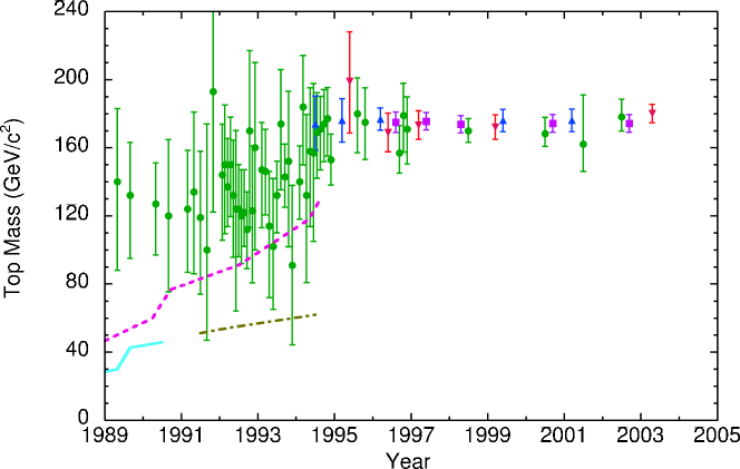
Fig. 2.: ($\diamondsuit$) Indirect bounds on the top-quark mass from precision electroweak data. ($\sqcap\!\!\!\!\sqcup$) World-average direct measurement of the top-quark mass; ($\bigtriangleup$) CDF and ($\bigtriangledown$) D0 measurements. Lower bounds from $p\bar{p}$ (dashed) and $e^{+}e^{-}$ (solid) colliders. Updated by C. Quigg from Ref. [11].

The precision electroweak data became much more precise in 1989 with the advent of the CERN Large Electron-Positron (LEP) collider and the Stanford Linear Collider (SLC). I show in Fig. 2 the top-quark mass extracted from precision electroweak analyses from 1989 to the present. As the data became more precise, and the lower bound from the Tevatron continued to increase, it became clear that the top quark is much heavier than expected. This culminated in the discovery of the top quark in 1995 [12, 13] with a mass around 175 GeV, in the range anticipated by precision electroweak analyses.

The top quark was not a central motivation for the S$p\bar{p}$S nor the Tevatron, but it proved to be one of the most important discoveries at these machines. We anticipated the existence of the top quark, and we used precision electroweak data to successfully determine the allowed mass range. This was a great success, and was part of the reason the 1999 Nobel Prize was awarded to G. ’t Hooft [14] and M. Veltman [15]. However, the large mass of the top quark was a real surprise.

Along the way, we developed new experimental techniques that could not have been dreamt of when the S$p\bar{p}$S and the Tevatron were being designed. For the top quark, the ability to tag $b$ quarks using a silicon vertex detector (SVX) is a very powerful tool. It wasn’t until 1983 that we discovered that the $b$ quark has a surprisingly long lifetime [16, 17] that might allow one to detect a secondary vertex from $b$ decay. By the mid 1980’s it was well appreciated that this could be used to tag $b$ jets at hadron colliders, but the anticipated efficiency was quite low [18]. When the top quark was discovered in 1995, we learned that the efficiency for SVX $b$-tagging is as much as $50\%$, yet another surprise in the saga of the top quark.

2 The LHC

The central motivation for the LHC is to discover the mechanism of electroweak symmetry breaking. Recall that this mechanism is not specified in the spontaneously-broken $SU(2)_{L}\times U(1)_{Y}$ gauge theory. The amplitude for the scattering of $W$ bosons in that theory is shown in Fig. 3(a). In the standard model, one introduces a Higgs field that acquires a vacuum expectation value and breaks the electroweak symmetry. This results in a new particle in the theory, the Higgs boson. Thus there is an additional diagram, involving the exchange of the Higgs boson, that contributes to the amplitude for $W$-boson scattering, shown in Fig. 3(b). For energies less than the Higgs-boson mass, the effective theory is the spontaneously-broken $SU(2)_{L}\times U(1)_{Y}$ gauge theory. The effective theory above the Higgs-boson mass includes the Higgs field, which provides the mechanism for electroweak symmetry breaking. Thus it is appropriate to refer to the Higgs-boson mass as the “scale of electroweak symmetry breaking” in the standard model.

Fig. 3.: (a) The effective theory of the weak interaction at energies less than the Higgs mass is the spontaneously-broken $SU(2)_{L}\times U(1)_{Y}$ gauge theory; (b) at energies above the Higgs mass, the effective theory is the standard model.

In the spontaneously-broken $SU(2)_{L}\times U(1)_{Y}$ gauge theory without a specific mechanism for symmetry breaking, the gauge symmetry is realized nonlinearly. When a specific mechanism is introduced, the gauge symmetry is realized linearly. Thus the general definition of the “scale of electroweak symmetry breaking” is the scale above which the gauge symmetry of the effective theory is realized linearly. The standard model is a specific example of this general definition.

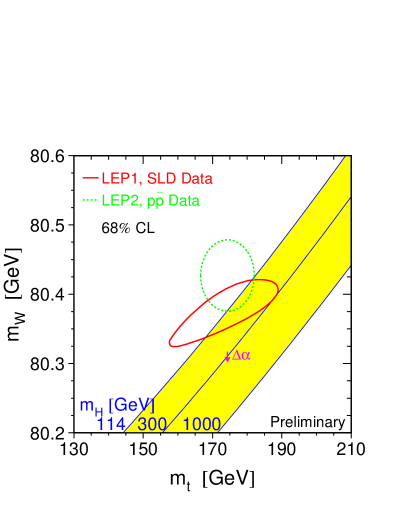
Fig. 4.: Lines of constant Higgs mass on a plot of $M_{W}$ vs. $m_{t}$. The dashed ellipse is the $68\%$ CL direct measurement of $M_{W}$ and $m_{t}$. The solid ellipse is the $68\%$ CL indirect measurement from precision electroweak data. From http://lepewwg.web.cern.ch/LEPEWWG.

Fig. 5.: Higgs-boson production (a) in association with a weak vector boson, (b) via weak-vector-boson fusion.

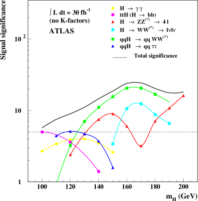
Fig. 6.: $S/\sqrt{B}$ for a variety of Higgs-boson production and decay channels at the LHC vs. the Higgs mass.

Let’s consider the possibility that the standard Higgs model is correct. Just as precision electroweak data honed in on the allowed range of the top-quark mass, we can use this data to determine the allowed range for the Higgs-boson mass. The precision electroweak data are summarized on a plot of the $W$ mass vs. the top-quark mass, shown in Fig. 4. Lines of constant Higgs mass are drawn on this plot. The elongated ellipse represents the precision electroweak data, assuming the standard Higgs model. The dashed ellipse indicates the direct measurement of the $W$ mass and the top-quark mass. The most striking thing about his plot is that the two ellipses overlap near the lines of constant Higgs mass. This did not have to happen: these two ellipses could have ended up anywhere on this plot (or even off of it), and they did not have to overlap. This indicates that the standard Higgs model is at least a good approximation to reality. Furthermore, the ellipses overlap near the lines of constant Higgs mass corresponding to small values of the Higgs mass. This indicates that the Higgs boson is not much heavier than the present lower bound of $m_{h}>114.4$ GeV [19].

Such an intermediate-mass Higgs boson may be accessible in Run II at the Tevatron via the associated production of the Higgs boson and a weak vector boson, as shown in Fig. 5(a) [20]. This is remarkable because the Higgs boson was not at all a motivation for the Tevatron. This search channel only became feasible once we realized that we could tag $b$ jets with high efficiency, since the Higgs boson decays dominantly to $b\bar{b}$ in the Higgs-mass region of interest. The discovery of the Higgs boson via this process requires a lot of integrated luminosity [21, 22]. However, we should keep in mind that our projections about the required luminosity for a given measurement are sometimes too conservative. A striking example is the projected accuracy in the measurement of the top-quark mass made in the TeV-2000 study in 1996, $\delta m_{t}=13$ GeV (with 70 pb^-1 of data) [21]. Just two years later CDF and D0 measured the mass with a combined accuracy of 5.1 GeV (with 100 pb^-1 of data) [23]. We greatly underestimated the sensitivity of the measurement, despite the fact that at the time we probably thought we were being optimistic. The lesson is that “data make you smarter” [24].

Studies also make you smarter. In the context of an intermediate-mass Higgs boson, this is exemplified by the production of the Higgs boson via weak-vector-boson fusion, shown in Fig. 5(b). This process was originally thought to be of interest primarily for a heavy Higgs boson, $m_{h}>2M_{W}$ [25]. However, in recent years it has been realized that it is also very important for an intermediate-mass Higgs boson [26]. I show in Fig. 6 the signal significance for an intermediate-mass Higgs boson at the LHC via a variety of production and decay channels. The importance of the weak-vector-boson channels is evident from this plot.

3 The view through the sunroof

Figure 7 shows the WMAP data on the temperature fluctuations in the cosmic microwave background radiation [27]. Cosmological parameters can be extracted from this data with impressive precision. The total energy density of the universe, in units of the critical density, is very close to unity,

$$\mathchar 266\relax_{TOT}=\mathchar 266\relax_{B}+\mathchar 266\relax_{DM}+\mathchar 266\relax_{\mathchar 259\relax}=1.02\pm 0.02\;,$$

where $\mathchar 266\relax_{B}$, $\mathchar 266\relax_{DM}$, $\mathchar 266\relax_{\mathchar 259\relax}$ are the baryon, dark-matter, and dark-energy densities in units of the critical density,

$$\mathchar 266\relax_{B} = 0.044\pm 0.004$$

$$\mathchar 266\relax_{DM} = 0.22\pm 0.04$$

$$\mathchar 266\relax_{\mathchar 259\relax} = 0.73\pm 0.04\;.$$

We have known about the existence of dark matter for a long time, and now the dark-matter density is known with good accuracy. Dark energy has come and gone throughout the decades, but now it looks like it is here to stay. In addition, $\mathchar 266\relax_{TOT}\approx 1$ and other features of the data are consistent with inflation.

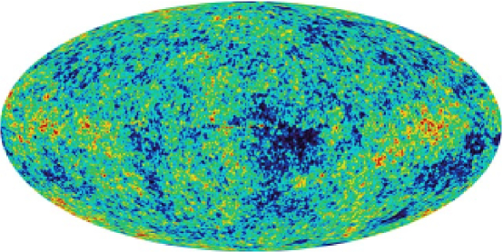
Fig. 7.: Temperature fluctuations in the cosmic microwave background as seen by WMAP. From Ref. [27].

Could we find dark matter at the LHC? The discovery of dark matter was not one of the original motivations for the LHC — there is no mention of it in the proceedings of the 1982 Snowmass study that gave birth to the SSC [28] — although it later became one of the goals of the project [29]. However, the discovery of dark matter, which makes up 22% of the universe, is potentially more exciting than understanding the mechanism of electroweak symmetry breaking.

Supersymmetry (SUSY) provides an attractive candidate for the dark matter, the “neutralino,” which is a linear combination of the photino, Zino, and Higgsinos. If it is the lightest supersymmetric particle, and $R$ parity is conserved, then it is stable. However, now that we know the dark-matter density with good accuracy, it turns out that supersymmetry generically produces too much dark matter. Figure 8 shows the regions of SUSY parameter space that are consistent with the dark-matter density, before and after the WMAP data. Before the WMAP data, there were large regions allowed, but after the data there are only slivers of parameter space that survive. This is noteworthy because these slivers represent regions in which special coincidences occur that allow the dark matter to annihilate. In the top two diagrams of Fig. 8, the slivers extending towards the right represent the case where the supersymmetric partner of the tau lepton is nearly degenerate with the neutralino, so it is present in sufficient abundance for co-annihilation to occur (e.g., $\chi^{0}\tilde{\tau}_{1}\to\gamma\tau$). In the bottom two diagrams, the slivers correspond to the neutralino mass being close to half the mass of a Higgs boson, such that annihilation occurs via the Higgs resonance. In the first of these two diagrams, there are two slivers — in the “funnel” between them, too much dark matter is annihilated. This is the most natural solution; one must be close to a Higgs resonance, but not right on top of it, to get the correct relic abundance of dark matter. Another natural solution, at very large values of $m_{0}$ (not shown in the figures), is the “focus-point” region [31].

Fig. 8.: The $(m_{1/2},m_{0})$ planes for (a) $\tan\beta=10,\mu>0$, (b) $\tan\beta=10,\mu<0$, (c) $\tan\beta=35,\mu<0$, and (d) $\tan\beta=50,\mu>0$ ($A_{0}=0$ in all cases). In each panel, the region allowed by the older cosmological constraint $0.1\leq\mathchar 266\relax_{\chi}h^{2}\leq 0.3$ has medium shading, and the region allowed by the newer cosmological constraint $0.094\leq\mathchar 266\relax_{\chi}h^{2}\leq 0.129$ has very dark shading. The disallowed region where $m_{\tilde{\tau}_{1}}<m_{\chi}$ has dark (red) shading. The regions excluded by $b\rightarrow s\gamma$ have medium (green) shading. (The regions of medium (pink) shading in panels (a,d), formerly favored by $g_{\mu}-2$, are now obsolete.) A dot-dashed line in panel (a) delineates the LEP constraint on the $\tilde{e}$ mass and the contours $m_{\chi^{\pm}}=104$ GeV ($m_{h}=114$ GeV) are shown as near-vertical black dashed (red dot-dashed) lines in panel (a) (each panel). From Ref. [30].

Dark energy is much harder to explain than dark matter. Like dark matter, dark energy was not anticipated. As far as we can tell, dark energy is a constant over space, and acts like a cosmological constant, $\mathchar 259\relax$. It is hard to understand why $\mathchar 259\relax\ll M_{P}^{2}$ ($M_{P}$ is the Planck scale), or even why $\mathchar 259\relax\ll v^{2}$ ($v$ is the Higgs-field vacuum expectation value). For many years it was assumed that $\mathchar 259\relax$ is exactly zero, and that we would some day discover the mechanism that ensures that it vanishes. Now we have the harder problem of explaining why it is so small and yet not exactly zero [32].

Another thing we learn by looking through the sunroof is that neutrinos, both solar and atmospheric, oscillate. This implies that neutrinos have a small mass. Like dark matter and dark energy, this is physics beyond the standard model.

Table 1.: The fermions of the first generation. The right-handed neutrino field, $N_{R}$, is not present in the standard model.

$Q_{L}\equiv\left(\begin{array}[]{l}u_{L}\\ d_{L}\end{array}\right)$	$\begin{array}[]{l}u_{R}\\ d_{R}\end{array}$
$L_{L}\equiv\left(\begin{array}[]{l}\nu_{L}\\ e_{L}\end{array}\right)$	$\begin{array}[]{l}N_{R}\\ e_{R}\end{array}$

I show in Table 1 the fermions of the first generation. I have added a right-handed neutrino field, $N_{R}$, which is not present in the standard model. It is plausible that such a field exists — why should all the other left-handed fields have right-handed partners, but not the neutrino? However, this field is special, because it is the only one that does not have $SU(2)_{L}\times U(1)_{Y}$ interactions — it is completely inert. Unlike the other fields, which are forbidden from having a mass by the $SU(2)_{L}\times U(1)_{Y}$ gauge symmetry, the field $N_{R}$ is allowed to have a mass, and therefore we expect that it does. The other fields acquire a mass, via their coupling to the Higgs field, only when the $SU(2)_{L}\times U(1)_{Y}$ gauge symmetry is spontaneously broken. This is illustrated in Fig. 9(a) for the electron, where the left- and right-handed electron fields together acquire a Dirac mass proportional to their coupling to the Higgs field times the Higgs vacuum-expectation value.

Fig. 9.: (a) The electron acquires a Dirac mass via its coupling to the Higgs field, $y_{e}$; (b) the neutrino acquires a Majorana mass via the square of its coupling to the Higgs field, $y_{\nu}$, and an intermediate, heavy, right-handed neutrino.

Since the right-handed neutrino field has a mass, it does not simply pair up with the left-handed neutrino field to generate a Dirac mass. Instead, it generates a Majorana mass for the left-handed neutrino field, as shown in Fig. 9(b). This requires two interactions with the Higgs field, so the neutrino mass is proportional to the square of the coupling to the Higgs field times the square of the Higgs vacuum-expectation value, divided by the mass of the right-handed neutrino field (which enters via its propagator). If $M_{R}$ is much greater than $v$, then the neutrino is very light. Taking $M_{R}$ to be around the scale of grand unification yields neutrino masses in the range $10^{-5}-10^{2}$ eV [33], consistent with what we know from neutrino oscillation experiments. Thus we anticipated neutrino masses from grand unification. However, we did not anticipate the large observed mixing angles, $\theta_{12}\approx 34^{\circ}$, $\theta_{23}\approx 45^{\circ}$. Like the top quark, this is another example where we anticipated the general framework, but not the details.

4 Grand Unification

Fig. 10.: Gauge coupling unification in the minimal supersymmetric standard model.

Fig. 11.: Gauge coupling unification in the standard model with two Higgs doublets plus their supersymmetric partners. The same result is obtained in the standard model with six Higgs doublets. From Ref. [38].

Since neutrino masses support the framework of grand unification, let’s consider the status of such theories. The standard model fits neatly into $SU(5)$ [34], but the couplings fail to unify at the grand-unified scale. As is well know, coupling unification is successful if one extends the standard model to include supersymmetry in the minimal way [35, 36, 37], as shown in Fig. 10. What is less well known is that this is due entirely to the extension of Higgs sector to include a second Higgs doublet and the superpartners of the two Higgs doublets. To illustrate this point, I show in Fig. 11 the evolution of the gauge couplings obtained by adding just the second Higgs doublet and the Higgs superpartners. Exactly the same evolution is obtained in the standard model with six Higgs doublets [38]. However, the unification scale is around $10^{14}$ GeV, which implies rapid proton decay in the $SU(5)$ model. One of the attractive features of supersymmetry is that it not only allows for coupling unification, it also pushes the unification scale up to around $10^{16}$ GeV, making it safe from rapid proton decay [39].

Once we accept the existence of the right-handed neutrino field, $N_{R}$, it is attractive to consider $SO(10)$ as the grand-unified gauge group [40, 41]. The fermions of a single generation fit into the $\bar{5}+10+1$ representation of $SU(5)$, where the $1$ is the $N_{R}$ field, which is simply tacked onto the theory. In contrast, the fermions of a single generation fill out the $16$ representation of $SO(10)$. Thus $SO(10)$ is more unified than $SU(5)$. It is possible that $SO(10)$ is spontaneously broken to $SU(5)$ at or above the grand-unified scale, in which case we are led back to the $SU(5)$ scenario discussed above. However, there are other possible symmetry-breaking patterns, which do not necessarily require weak-scale supersymmetry. A non-supersymmetric example is $SO(10)\to SU(4)_{c}\times SU(2)_{L}\times SU(2)_{R}\to SM$ [42]. In order to achieve coupling unification, there is an intermediate scale of symmetry breaking between the weak scale and the grand-unified scale [43]. Since this intermediate scale is adjusted to yield coupling unification, we lose the prediction of the weak mixing angle that is one of the successes of the supersymmetric $SU(5)$ theory.

Another reason weak-scale supersymmetry is attractive is that it stabilizes the hierarchy $m_{h}\ll M_{U}$, where $M_{U}$ is the unification scale (although it does not explain why the hierarchy exists). This stabilization results from the cancellation of quadratically-divergent corrections to the Higgs-boson mass from loops of particles and their supersymmetric partners, as shown in Fig. 12 [44, 45, 46]. However, weak-scale supersymmetry fails to stabilize the hierarchy $\mathchar 259\relax\ll v^{2}$, so it seems we are still missing a big part of the picture.

Fig. 12.: Quadratic divergences from loops of particles and their supersymmetric partners cancel in supersymmetric theories, exemplified here by Higgs and Higgsino loops.

I believe that $SO(10)\to SU(5)\to SM$ with weak-scale supersymmetry is the most attractive theory we’ve got, but it is unlikely that we have anticipated all the details, just as we failed to anticipate the top-quark mass and the neutrino mixing angles. The LHC will decide if weak-scale supersymmetry is really an outpost on the path to grand unification, or simply a mirage.

5 The Higgs Boson

As I discussed above, the LHC was designed to discover the mechanism of electroweak symmetry breaking. The evidence suggests that this involves a Higgs field (or fields) that acquires a vacuum-expectation value. Here I would like to list the intellectual reasons why the discovery of the Higgs boson (or bosons) is so important:

• We have no experience in particle physics with a fundamental scalar field, nor with a scalar field that acquires a vacuum-expectation value. We do have experience with a composite field that acquires a vacuum-expectation value in QCD, $\langle\bar{q}q\rangle$, where $q$ is a quark field. This breaks the chiral symmetry of QCD down to isospin. The analogue of this mechanism for electroweak symmetry breaking is called Technicolor, and is an alternative to a fundamental scalar field [47, 48].

  

  Fig. 13.: Like the graviton and the gauge bosons of the standard model, the Higgs boson mediates a fundamental force of nature.

• The Higgs boson mediates a new force of nature, just as the graviton mediates the gravitational force and the gauge bosons of the standard model mediate the strong and electroweak forces, as shown in Fig. 13. Unlike the graviton, which has spin 2, and the gauge bosons, which have spin 1, the Higgs boson has spin 0, since it is a scalar field.

• The Higgs field is responsible CKM mixing and $CP$ violation. The quarks acquire mass via their coupling to the Higgs field,

  $${\cal L}_{Yukawa}=\mathchar 256\relax^{ij}_{u}\bar{Q}_{L}^{i}\epsilon\phi^{*}u_{R}^{j}+\mathchar 256\relax^{ij}_{d}\bar{Q}_{L}^{i}\phi d_{R}^{j}$$

  ($Q_{L}$ is defined in Table 1) where the indicies $i,j=1,2,3$ indicate the generation. The fact that the Yukawa matrices $\mathchar 256\relax_{u},\mathchar 256\relax_{d}$ are nondiagonal leads to CKM mixing, and the fact that they are complex yields $CP$ violation. An analogous mechanism leads to MNS mixing in the lepton sector (evidenced via neutrino oscillations), as well as leptonic $CP$ violation (yet to be observed). We would like to understand the curious pattern of fermion masses and mixing observed in nature.

• We don’t understand why the cosmological constant is so much less than the vacuum-expectation value of the Higgs field, $\mathchar 259\relax\ll v^{2}$. One might imagine that there is some mechanism that forces it to zero, but then we have to explain why it is observed to be nonzero. “Quintessence” is another scalar field introduced to provide such an explanation [32].

• The WMAP measurements provide support for inflation, but we do not know the dynamics that drive inflation. Yet another scalar field, the “inflaton,” has been proposed for that purpose.

• As discussed above, gauge-coupling unification relies on the Higgs field (or fields). There may be yet more Higgs fields responsible for spontaneously breaking the grand-unified symmetry.

These observations show that the Higgs boson is not only central to the standard model, it is central to physics beyond the standard model. The LHC promises to open up an entirely new chapter in our quest to understand nature at a deeper level.

6 The Road Ahead

We still have a long road ahead of us, but it is worth the wait. As we approach our destination, we will encounter a landscape that is familiar in some ways, exotic in others. Recall that when the CERN $Sp\bar{p}S$ first began operation, there was a lot of confusion: monojets, a 40 GeV top quark, and so on. I believe that when we begin the operation of the LHC, the situation will be both confusing and exhilarating. It will require the best efforts of us all to make sense of it.

References

- 1. G. Arnison et al. [UA1 Collaboration], Phys. Lett. B 122, 103 (1983).
- 2. G. Arnison et al. [UA1 Collaboration], Phys. Lett. B 126, 398 (1983).
- 3. M. Banner et al. [UA2 Collaboration], Phys. Lett. B 122, 476 (1983).
- 4. P. Bagnaia et al. [UA2 Collaboration], Phys. Lett. B 129, 130 (1983).
- 5. C. Rubbia, Rev. Mod. Phys. 57, 699 (1985).
- 6. S. Van Der Meer, Rev. Mod. Phys. 57, 689 (1985).
- 7. S. W. Herb et al., Phys. Rev. Lett. 39, 252 (1977).
- 8. H. J. Behrend et al. [CELLO Collaboration], Phys. Lett. B 144, 297 (1984).
- 9. G. Arnison et al. [UA1 Collaboration], Phys. Lett. B 147, 493 (1984).
- 10. U. Amaldi et al., Phys. Rev. D 36, 1385 (1987).
- 11. C. Quigg, Phys. Today 50N5, 20 (1997).
- 12. F. Abe et al. [CDF Collaboration], Phys. Rev. Lett. 74, 2626 (1995) [arXiv:hep-ex/9503002].
- 13. S. Abachi et al. [D0 Collaboration], Phys. Rev. Lett. 74, 2632 (1995) [arXiv:hep-ex/9503003].
- 14. G. ’t Hooft, Rev. Mod. Phys. 72, 333 (2000) [Erratum-ibid. 74, 1343 (2003)].
- 15. M. J. Veltman, Rev. Mod. Phys. 72, 341 (2000).
- 16. E. Fernandez et al., Phys. Rev. Lett. 51, 1022 (1983).
- 17. N. Lockyer et al., Phys. Rev. Lett. 51, 1316 (1983).
- 18. J. E. Brau, K. T. Pitts and L. E. Price, in Proceedings of the 1988 DPF Summer Study on High-energy Physics in the 1990s (Snowmass 88), Snowmass, Colorado, 27 Jun - 15 Jul, 1988, ed. S. Jensen, p. 103.
- 19. ALEPH, DELPHI, L3, and OPAL Collaborations, The LEP Working Group for Higgs Boson Searches, CERN-EP/2003-011.
- 20. A. Stange, W. J. Marciano and S. Willenbrock, Phys. Rev. D 49, 1354 (1994) [arXiv:hep-ph/9309294].
- 21. D. Amidei et al. [TeV-2000 Study Group Collaboration], FERMILAB-PUB-96-082
- 22. M. Carena et al. [Higgs Working Group Collaboration], arXiv:hep-ph/0010338.
- 23. L. Demortier, R. Hall, R. Hughes, B. Klima, R. Roser and M. Strovink [The Top Averaging Group Collaboration], FERMILAB-TM-2084
- 24. D. Amidei and C. Brock, FERMINEWS 26, No. 1, p. 6 (January 17, 2003) [http://www.fnal.gov/pub/ferminews/ferminews03-01-17/p3.html].
- 25. R. N. Cahn and S. Dawson, Phys. Lett. B 136, 196 (1984) [Erratum-ibid. B 138, 464 (1984)].
- 26. D. Rainwater and D. Zeppenfeld, JHEP 9712, 005 (1997) [arXiv:hep-ph/9712271].
- 27. C. L. Bennett et al., arXiv:astro-ph/0302207.
- 28. Proceedings of the 1982 DPF Summer Study on Elementary Particle Physics and Future Facilities (Snowmass 82), Snowmass, Colorado, 28 Jun - 16 Jul, 1982, eds. R. Donaldson, R. Gustafson, and F. Paige.
- 29. C. Quigg and R. F. Schwitters, Science 231, 1522 (1986).
- 30. J. R. Ellis, K. A. Olive, Y. Santoso and V. C. Spanos, arXiv:hep-ph/0303043.
- 31. J. L. Feng, K. T. Matchev and F. Wilczek, Phys. Lett. B 482, 388 (2000) [arXiv:hep-ph/0004043].
- 32. S. M. Carroll, arXiv:astro-ph/0107571.
- 33. P. Langacker, Phys. Rept. 72, 185 (1981).
- 34. H. Georgi and S. L. Glashow, Phys. Rev. Lett. 32, 438 (1974).
- 35. J. R. Ellis, S. Kelley and D. V. Nanopoulos, Phys. Lett. B 260, 131 (1991).
- 36. U. Amaldi, W. de Boer and H. Furstenau, Phys. Lett. B 260, 447 (1991).
- 37. P. Langacker and M. Luo, Phys. Rev. D 44, 817 (1991).
- 38. S. Willenbrock, Phys. Lett. B 561, 130 (2003) [arXiv:hep-ph/0302168].
- 39. S. Dimopoulos, S. Raby and F. Wilczek, Phys. Rev. D 24, 1681 (1981).
- 40. H. Georgi, AIP Conf. Proc. 23, 575 (1975).
- 41. H. Fritzsch and P. Minkowski, Annals Phys. 93, 193 (1975).
- 42. J. C. Pati and A. Salam, Phys. Rev. D 10, 275 (1974).
- 43. N. G. Deshpande, E. Keith and P. B. Pal, Phys. Rev. D 46, 2261 (1993).
- 44. M. J. Veltman, Acta Phys. Polon. B 12, 437 (1981).
- 45. L. Maiani, in Proceedings of the Summer School on Particle Physics, Gif-Sur-Yvette, 1979, edited by G. Altarelli (IN2P3, Paris, 1980), p. 1.
- 46. E. Witten, Nucl. Phys. B 188, 513 (1981).
- 47. S. Weinberg, Phys. Rev. D 19, 1277 (1979).
- 48. L. Susskind, Phys. Rev. D 20, 2619 (1979).