Leptonic universality breaking in $\Upsilon$ decays as a probe of new physics

Abstract

In this work we examine the possible existence of new physics beyond the standard model which could modify the branching fractions of the leptonic (mainly tauonic) decays of bottomonium vector resonances below the $B\bar{B}$ threshold. The decay width is factorized as the product of two pieces: a) the probability of an intermediate pseudoscalar color-singlet $b\bar{b}$ state (coupling to the dominant Fock state of the Upsilon via a magnetic dipole transition) and a soft (undetected) photon; b) the annihilation width of the $b\bar{b}$ pair into two leptons, mediated by a non-standard CP-odd Higgs boson of mass about $10$ GeV, introducing a quadratic dependence on the lepton mass in the partial width. The process would be unwittingly ascribed to the $\Upsilon$ leptonic channel thereby (slightly) breaking lepton universality. A possible mixing of the pseudoscalar Higgs and bottomonium resonances is also considered. Finally, several experimental signatures to check out the validity of the conjecture are discussed.

PACS numbers: 14.80.Cp, 13.25.Gv, 14.80.-j
Keywords: Non-standard Higgs, New Physics, bottomonium leptonic decays, lepton universality

1 Introduction

The Standard Model (SM) has become nowadays the necessary reference to confront experimental data with theory: any possible discrepancy between them is commonly denoted as New Physics (NP), actually implying the need for some new assumptions or extensions of the basic physical postulates. In the SM, matter and gauge fields follow different statistics, the former being fermions and the latter bosons. As is well-known, there are important reasons to believe that this is quite unsatisfactory. One of the major motivations to extend the SM is to resolve the hierarchy and fine-tuning questions between the electroweak scale and the Planck scale. Supersymmetry is a very nice solution in this regard, since diagrams with superpartners exactly cancel the quadratic divergences of the SM diagrams. In particular, it requires that the boson sector of the SM including the Higgs structure should be enlarged with new scalar fields. Until recently, supersymmetry was thought as the only possibility to solve the hierarchy problem, partly because of the lack of known alternatives. However, a new formulation for the electroweak symmetry breaking (dubbed $``$little Higgs” theories [1]) has recently emerged where cancellation of divergences occur, conversely to supersymmetry, between particles with the same statistics. The (initially massless) Higgs fields can be seen in this framework as Goldstone bosons, adquiring a mass and becoming pseudo-Goldstone bosons via explicit symmetry breaking at the electroweak scale, but still protected by an approximate global symmetry which would keep them relatively light.

This is not the whole story, however. Another approach to solve the hierarchy problem aimed to the old idea on Kaluza-Klein extra dimensions, either in an ADD scenario [2, 3] or in a Randall-Sundrum model [4]. In both cases, the scalar sector would be increased by the presence of neutral bosons like scalar gravitons and radions (the latter associated to the quantum oscillations of the interbrane separation), eventually leading to measurable deviations from the SM [5, 6]. Moreover, let us cite another example of this kind of extensions of the SM: the axion model, originally introduced in [7, 8] as a consequence of the spontaneous breaking of the global $U(1)_{PQ}$ axial symmetry. Nowadays, the axion is a pseudoscalar field appearing in a variety of theories with different meanings including superstring theory, yielding sometimes a massless particle and others a massive one: in astrophysics the axion represents a good candidate of the cold dark matter component of the Universe.

Although there are well established mass bounds (e.g. from LEP searches [9]) for the standard Higgs boson and the Minimal Supersymmetric Standard Model (MSSM), the situation can be different in more general scenarios where the tight constraints on the parameters of the theory do not apply, leaving still room for light Higgs bosons compatible with present data although the point is currently controversial (see, for example, [10, 11, 12, 13]). As a suggestive example, let us mention that a possible mixing between Higgs bosons from a two doublet structure (which will deserve special attention in this paper) and resonances would alter the exclusion limits put by LEP data on light Higgs bosons since the branching fraction (BF) into tau pairs decreases considerably in this case [10, 14]. Moreover, in the so-called next to MSSM (NMSSM) a gauge singlet superfield is added to the MSSM spectrum [15, 16]: new CP-even and CP-odd Higgs bosons enter the game. For some choices of the parameters of this model, one can obtain very light pseudoscalar Higgs states evading the LEP constraints and whose detection might require some dedicated efforts at the LHC [17].

The search for axions or light Higgs bosons in the decays of heavy resonances has several attractive features: first, the couplings of the former to fermions are proportional to their masses and therefore enhanced with respect to lighter mesons. Second, theoretical calculations are more reliable, notably with the advent of non-relativistic quantum chromodynamics (NRQCD) [18, 19]. Indeed, intensive searches for a light Higgs-like boson (to be generically denoted by $\phi^{0}$ in this paper) have been performed according to the so-called Wilczek mechanism [20] in the radiative decay of vector heavy quarkonia like the Upsilon resonance (i.e. $\Upsilon{\rightarrow}\ \gamma\phi^{0}$). To date, none of all these searches has been successful, but have provided valuable constraints on the mass values of light Higgs bosons [21].

Nevertheless, in this paper we develop the key ideas already presented in [22, 23] on a possible signal of NP based on the $``$apparent” breaking of lepton universality in bottomonium decays. Stricto sensu, lepton universality implies that the electroweak couplings to gauge fields of all charged lepton species should be the same; according to our interpretation, the (would-be) dependence on the leptonic mass of the leptonic branching fractions (${\cal B}_{\ell\ell}$ ; $\ell=e,\mu,\tau$) of $\Upsilon$ resonances below the $B\bar{B}$ threshold, if experimentally confirmed by forthcoming measurements, might be viewed as a hint of the existence of a quite light Higgs - of mass about 10 GeV - deserving a closer look.

1.1 Two-Higgs Doublet Models

In its minimal version, the SM requires a complex scalar weak-isospin doublet to spontaneously break the electroweak gauge symmetry. As already commented, theories that try to resolve the hierarchy and fine-tuning problems imply the extension of the Higgs sector. Loosely speaking, the simplest way (i.e. adding the fewest number of arbitrary parameters) corresponds to assume an extra Higgs doublet, i.e. the Two-Higgs Doublet Model (2HDM) [21]. The Higgs content of this theory is the following: a charged pair ($H^{\pm}$), two neutral CP-even scalars ($h^{0}$, $H^{0}$) and a neutral CP-odd scalar ($A^{0}$) often referred as a pseudoscalar. Let us also note that diverse extended frameworks beyond the SM can lead to an effective theory at low energies equivalent to the 2HDM. On the other hand, there exist models with higher representations for the Higgs sector (e.g. Higgs triplets or the above-mentioned NMSSM) leading to more complicated structures [24].

Any two-doublet Higgs model has to cope with the potential problem of enhancing the flavor-changing neutral currents (FCNC). Several solutions have been proposed to overcome this serious difficulty. In the Type-I 2HDM only one of the Higgs doublets couple to quarks and leptons and, since the process which diagonalizes the mass matrix of quarks equally can diagonalize the Higgs coupling, there is no flavor-changing vertex for the Higgs bosons at the end. (Note that in such case the Higgs coupling to $b$ quarks is not enhanced.) Another extreme possibility to avoid FCNC’s is based on the assumption that one Higgs doublet does not couple to fermions at all whereas the other Higgs’ couples to fermions in the same way as in the minimal Higgs model. On the other hand, the Type-II 2HDM allows one of the Higgs doublet couple to the up quarks and leptons while the other Higgs doublet can couple to down-type quarks and leptons. This is the kind of model on which we shall focus in the following, excluding MSSM since current limits rule out a very light pseudoscalar Higgs boson [9] as advocated along this work. Nevertheless, other alternative scenarios as those mentioned in the Introduction can not be discarded.

Among other new parameters of the 2HDM, one of special phenomenological significance in this work is the ratio of the vacuum expectation values ($v_{1,2}$ of the Higgs down- and up-doublets respectively) usually denoted as $\tan{\beta}=v_{2}/v_{1}$, where $v_{1}^{2}+v_{2}^{2}=v^{2}$ with $v\simeq 246$ GeV fixed by the $W$ mass. Indeed, $\tan{\beta}$ governs the Yukawa couplings between Higgs bosons and fermions, thereby potentially enhancing the rate of processes forbidden by the SM, but allowed thanks to new contributions heralding the existence of NP.

The layout of the paper is the following: in section 2 we tentatively introduce the hypothesis of a light non-standard Higgs boson which could modify the leptonic decay rate of $\Upsilon$ resonances; in section 3 we firstly apply time ordered second-order perturbation theory for a two-step process: prior photon radiation from the Upsilon leading to a pseudoscalar intermediate state followed by its annihilation into a lepton pair mediated by a CP-odd Higgs. Alternatively, we consider in subsection 3.2 the factorization of the decay width assuming the existence of Fock states in hadrons containing (ultra)soft photons as low-energy degrees of freedom in analogy to gluons in NRQCD. In sections 4 and 5, we focus on a 2HDM(II) model and the effects of the postulated NP contribution on the leptonic branching fraction are analyzed in the light of current experimental data: we conclude from a statistical test that lepton universality can be rejected at a 10$\%$ level of significance. Possible mixing between a pseudoscalar Higgs and $\eta_{b}$ resonances is also considered, and its consequences on the hyperfine splitting between vector and pseudoscalar states. We finally gather technical details in three appendices at the end of the paper.

2 Searching for a light Higgs-like boson in $\Upsilon$ leptonic decays

The starting point of our considerations is the well-known Van Royen-Weisskopf formula [25] including the color factor for the leptonic width of a vector quarkonium state without neglecting leptonic masses,

$${\Gamma}^{(em)}_{\Upsilon\to\ell\ell}\ =\ 4\alpha^{2}Q_{b}^{2}\ \frac{|R_{n}(0)|^{2}}{m_{\Upsilon}^{2}}\ {\times}\ K(x_{\ell})$$ (1)

where $\alpha\ {\simeq}\ 1/137$ is the electromagnetic fine structure constant; $m_{\Upsilon}$ denotes the mass of the vector particle (a $\Upsilon(nS)$ resonance in this particular case) and $Q_{b}$ is the charge of the relevant (bottom) quark ($1/3$ in units of $e$); $R_{n}(0)$ stands for the non-relativistic radial wave function of the $b\overline{b}$ bound state at the origin; finally, the $``$kinematic” factor $K$ reads

$$K(x_{\ell})\ =\ (1+2x_{\ell})(1-4x_{\ell})^{1/2}$$ (2)

where $x_{\ell}=m_{\ell}^{2}/m_{\Upsilon}^{2}$. Leptonic masses are usually neglected in Eq.(1) (by setting $K$ equal to unity) except for the decay into $\tau^{+}\tau^{-}$ pairs. Let us note that $K(x_{\ell})$ is a decreasing function of $x_{\ell}$: the higher leptonic mass the smaller decay rate. Such $x_{\ell}$-dependence is quite weak for bottomonium and, consequently, we will assume that lepton universality implies the constancy of the width (1) for all lepton species.

However, in this work we are conjecturing the existence of a light Higgs-like particle whose mass would be close to the $\Upsilon$ mass and which could show up in the cascade decay:

$$\Upsilon\ {\rightarrow}\ \gamma\ \phi^{0}({\rightarrow}\ \ell^{+}\ell^{-})\ \ \ ;\ \ \ \ell=e,\mu,\tau$$ (3)

Actually, this process may be seen as a continuum radiative transition that in principle permits the coupling of the bottom quark-antiquark pair to a particle of variable mass and $J^{PC}$: $0^{++},0^{-+},1^{++},2^{++}...$ (always positive charge conjugation). In this investigation we will confine our attention to the two first possibilities: a scalar or a pseudoscalar boson. In fact, intermediate bound states and not the continuum will play a leading role in the process, as we shall see. In the language of perturbation theory, a magnetic dipole transition (M1) would yield at leading order a pseudoscalar $b\bar{b}$ state from the initial-state vector resonance, subsequently annihilating into a dilepton. Alternatively, there should be a certain probability that a pseudoscalar color-singlet $b\bar{b}$ system could exist in the Fock decomposition of the physical Upsilon state, as the light degrees of freedom would carry the remaining quantum numbers.

Throughout this work, we will focus on vector $\Upsilon$ states of the bottomonium family below open flavor , and the complete process (3) actually would be

$$\Upsilon\rightarrow\gamma_{s}\,b\bar{b}[n](\rightarrow\phi^{0}\rightarrow\ell^{+}\ell^{-})\,\,\ ;\,\,\ \ell=e,\mu,\tau$$ (4)

where $\gamma_{s}$ denotes a soft (= unobserved) photon and $b\bar{b}[n]$ stands for those intermediate states of different quantum numbers collectively denoted by $n$, either on the continuum or as bound states. Note that $\phi^{0}$ is not a real particle in the channel (4), conversely to the Wilczek mechanism [20], but a virtual state mediating the annihilation of a $b\bar{b}$ intermediate state into the final-state lepton pair. Hence, if the $\phi^{0}$ mass were quite close to the $\Upsilon$ mass, the Higgs propagator could enhance significantly the width of whole process. In fact, the analysis performed by OPAL [10] using LEP data assuming a mixing between Higgs bosons and bottomonium resonances [14] does not permit to exclude a light Higgs of mass around 10 GeV using reasonable $\tan{\beta}$ values in the 2HDM(II). Moreover, one should not dismiss other possible scenarios, as pointed out in the Introduction.

Since the radiated photon would escape detection in our guess , the NP channel (4) would be unwittingly ascribed to the leptonic decay mode of the Upsilon resonance, introducing in its ${\cal B}_{\ell\ell}$ a quadratic leptonic mass dependence opposite to that of Eq.(2) due to the Higgs coupling to fermions This is a cornerstone in our conjecture but likely of practical significance only for the $\tau^{+}\tau^{-}$ decay mode, where missing energy is experimentally required as one of the selection criteria[27]: events with photons of order 100 MeV would be included in the sample of tauonic decays, ultimately contributing to the measured leptonic BF. On the contrary, the electronic and muonic BF’s would be affected to a much lesser extent, both because of: i) the smaller leptonic mass; ii) the experimental constraint on the reconstructed dilepton invariant mass, which restricts severely the energy of possible $``$lost” photons .

3 Intermediate $b\bar{b}$ pseudoscalar states

Along this section, we examine the role played by intermediate states in the process (4) according to two different schemes: firstly, we use time-ordered perturbation theory (TOPT) to deal with the formation, via an electromagnetic transition from the initial-state $\Upsilon$, of a virtual $b\bar{b}$ state and its subsequent annihilation into a lepton pair. As an alternative approach, we rely on the separation between long- and short-distance physics following the main lines of a non-relativistic effective theory (NRET) like NRQCD [19] - albeit replacing a gluon by a photon in the usual Fock decomposition of hadronic bound states - and NRQED [29, 30]. Different results for the final widths in each approach come up, however; they are discussed in subsection 3.3. Finally, let us note that, despite we generically refer to the Upsilon ($\Upsilon$) in our study, actually we are focusing on the $\Upsilon(1S)$ state because of more precise data on its tauonic BF (${\cal B}_{\tau\tau}$) w.r.t. the $\Upsilon(2S)$, and not yet available for the $\Upsilon(3S)$.

3.1 Time-ordered perturbative calculation

Let us write the amplitude for the process (4) using TOPT at lowest order:

$$T_{\,\Upsilon\to\gamma_{s}\,\ell\ell}=\sum_{n}\frac{\langle\,\ell^{+}\ell^{-}|\,{\mbox{H}}\,|\,n\,\rangle\langle\,\gamma_{s}\,n\,|\,{\mbox{H}}\,|\,\Upsilon\,\rangle}{m_{\Upsilon}-E_{n}-k+i\epsilon}$$ (5)

The sum extends over all possible $b\bar{b}$ intermediate states with proper quantum numbers and energy $E_{n}$, and $k$ is the energy of the unobserved photon. Bottomonium states in a ${}^{1}S_{0}$ configuration should dominate the sum, as we are facing the radiative decay of a $\Upsilon$ resonance. Intermediary states of higher angular momentum will be suppressed, since the associated electromagnetic transitions would involve higher multipole moments; M1 transitions to $S$-wave states with different principal quantum numbers will neither be considered, as they involve orthogonal wave functions in the non-relativistic limit.

From expression (5) we also see that intermediate states with energies closer to the $\Upsilon$ mass are enhanced with respect to those of higher virtuality. In that sense, the continuum $b\bar{b}$ contribution, starting with a pair of $B\bar{B}$ mesons ($E_{B\bar{B}}\simeq 10.56$ GeV), is well above the $\Upsilon(1S)$ and $\Upsilon(2S)$ masses, and the main contributions to the decay would come from intermediate pseudoscalar $S$-wave bound states, i.e. the $\eta_{b}$ resonances, differing from the $\Upsilon$ resonances in virtue of the hyperfine structure.

Squaring the amplitude (5) and including phase space integrations, the width of the process reads

$$\Gamma_{\,\Upsilon\to\gamma_{s}\,\ell\ell} = \int dk\,\rho_{\gamma}\left|\frac{\langle\,\eta_{b}\,\gamma_{s}\,|\,{\mbox{H}}\,|\,\Upsilon\,\rangle}{m_{\Upsilon}-E_{\eta}-k+i\epsilon}\right|^{2}$$ (6)

$$\times\int dE_{\ell\ell}\,\,\rho_{\ell^{+}\ell^{-}}\,|\langle\,\ell^{+}\ell^{-}|\,{\mbox{H}}\,|\,\eta_{b}\,\rangle|^{2}\,2\pi\,\delta(m_{\Upsilon}-k-E_{\ell\ell})+\dots$$

where the dots stand for other intermediate states contributing to the sum in (5). For explicit expressions of the particle densities $\rho_{\gamma}$, $\rho_{\ell^{+}\ell^{-}}$, we refer the reader to [31]. The last integral amounts to the width of a $0^{-+}$ resonance with mass $m_{\eta_{b}^{*}}=m_{\Upsilon}-k$ decaying into a pair of leptons, which we will denote as $\Gamma_{\eta_{b}^{*}\to\ell\ell}$. Section 4 will be devoted to the calculation of this annihilation via the proposed Higgs exchange.

The matrix element squared for the M1 transition between spin-triplet and spin-singlet $S$-wave states of quarkonium can be written in terms of the $\Upsilon(nS)\to\gamma_{s}\,\eta_{b}^{*}(nS)$ width after performing the integration over allowed photon states with energy $k$,

$$2\pi\int\rho_{\gamma}\,\left|\langle\,\eta_{b}\,\gamma_{s}\,|\,{\mbox{H}}\,|\,\Upsilon\,\rangle\right|^{2}\ =\ \Gamma^{\,M1}_{\,\Upsilon\to\gamma_{s}\,\eta_{b}^{*}}\ \simeq\ \frac{16\alpha}{3}\Big{(}\frac{Q_{b}}{2m_{b}}\Big{)}^{2}k^{3}$$ (7)

where we emphasize the off-shellness of pseudoscalar resonance by writing $\eta_{b}^{*}$. In the last step, we used a non-relativistic approximation to estimate the width $\Gamma^{\,M1}_{\,\Upsilon\to\gamma_{s}\,\eta_{b}^{*}}$ [32]. We shall return later to this formula in greater detail. Plugging the above result into Eq.(6) one obtains

$$\Gamma_{\,\Upsilon\to\gamma_{s}\,\ell\ell}\ =\ \frac{16\alpha}{3}\Big{(}\frac{Q_{b}}{2m_{b}}\Big{)}^{2}\frac{1}{2\pi}\int_{0}^{\Lambda}dk\,\frac{k^{3}}{\left|m_{\Upsilon}-E_{\eta_{b}}-k+i\epsilon\right|^{2}}\,\,\Gamma_{\eta_{b}^{*}\to\ell\ell}$$ (8)

Under the soft photon hypothesis, we have restricted the integration over photon energies to an upper limit $\Lambda\ll m_{\eta_{b}}$, dictated by both experimental photon energy resolution and event selection criteria as pointed out in section 2. In that case we can safely retain the first term in the expansion of the $\eta_{b}$ energy, $E_{\eta_{b}}\ =\ \sqrt{m_{\eta_{b}}+k^{2}}\simeq m_{\eta_{b}}+k^{2}/2m_{\eta_{b}}+...$ in the denominator of (8):

$$\Gamma_{\,\Upsilon\to\gamma_{s}\,\ell\ell}=\frac{16\alpha}{3}\Big{(}\frac{Q_{b}}{2m_{b}}\Big{)}^{2}\,\bigg{\{}\frac{1}{2\pi}\int_{0}^{\Lambda}dk\,\frac{k^{3}}{\left|m_{\Upsilon}-m_{\eta_{b}}+i\Gamma_{\eta_{b}}/2-k\right|^{\,2}}\ \Gamma_{\eta_{b}^{*}\to\ell\ell}\bigg{\}}$$ (9)

The instability of the $\eta_{b}$ intermediate state has been taken into account by the substitution $m_{\eta_{b}}\to m_{\eta_{b}}-i\Gamma_{\eta_{b}}/2$, valid in the narrow-width case. A rough estimate of this width can be obtained through the pQCD relation [32]

$$\frac{\Gamma_{\eta_{b}}}{\Gamma_{\eta_{c}}}\simeq\frac{m_{b}}{m_{c}}\left[\frac{\alpha_{s}(m_{b})}{\alpha_{s}(m_{c})}\right]^{5}$$

With reasonable values of the quark masses, the running strong coupling and the measured $\Gamma_{\eta_{c}}=16\pm 3\,$MeV [28], we get $\Gamma_{\eta_{b}}\simeq 4\,$MeV.

Consider now the quantity between curly braces in Eq.(9):

$$\frac{1}{2\pi}\int_{0}^{\Lambda}dk\,\frac{k^{3}}{(m_{\Upsilon}-m_{\eta_{b}}-k)^{2}+\Gamma_{\eta_{b}}^{2}/4}\ \Gamma_{\eta_{b}^{*}\to\ell\ell}\equiv{\cal I}(\Lambda,\Delta E_{hs})$$ (10)

The mass difference $m_{\Upsilon}-m_{\eta_{b}}\equiv\Delta E_{hs}$ is the hyperfine splitting between the $\Upsilon(nS)-\eta_{b}(nS)$ partners. Different approaches suggest that $\Delta E_{hs}$ lies in the interval $\sim 35-150$ MeV for $n=1$ (see [33] for a compilation of theoretical results). If $\Lambda>\Delta E_{hs}+\Gamma_{\eta_{b}}$, i.e. the range of energies for the unobserved photon is higher that the mass difference $\Delta E_{hs}$, the integration region in Eq.(10) comprises the full $\eta_{b}$ resonance contribution; taking $\Lambda\simeq\Delta E_{hs}$ would reduce the result by a half, and values of $\Lambda$ below $\Delta E_{hs}-\Gamma_{\eta_{b}}$ would make ${\cal I}$ almost vanishing. Finally, a very large value of $\Lambda$ would make (10) quadratically divergent (and then $\Lambda$ can be seen as an ultraviolet regulator).

Now, keeping track of our discussion at the end of section 2, those events with photons of energies up to several hundred MeV would pass the selection criteria employed in experiments measuring the tauonic BF of $\Upsilon$ resonances. Therefore, one can safely take in this case ($\ell=\tau$) the upper limit $\Lambda$ in the integrals of Eqs. (8-10) of the order of few hundreds of MeV, well above the quantity $\Delta E_{hs}+\Gamma_{\eta_{b}}$, but always $\Lambda\ll m_{\eta_{b}}$.

We thus evaluate the integral in Eq.(10) and take the limit of small $\Gamma_{\eta_{b}}$, yielding

$${\cal I}(\Lambda,\Delta E_{hs})\ \simeq\ \frac{(\Delta E_{hs})^{3}}{\Gamma_{\eta_{b}}}\ \Gamma_{\eta_{b}\to\ell\ell}$$

The off-shell width $\Gamma_{\eta_{b}^{*}\to\ell\ell}$ has been transformed in this limit to the on-shell width $\Gamma_{\eta_{b}\to\ell\ell}$, as $m_{\eta_{b}^{*}}=m_{\Upsilon}-\Delta E_{hs}=m_{\eta_{b}}$. In section 4 we will obtain an expression for this partial width dominated by the postulated Higgs boson.

Finally, under the aforementioned assumption that the photon energy cutoff $\Lambda$ is large enough, the partial width of the whole decay reduces to the factorized formula

$$\Gamma_{\,\Upsilon\to\gamma_{s}\,\ell\ell}\ =\ \Gamma^{\,M1}_{\,\Upsilon\to\gamma_{s}\eta_{b}}\frac{\Gamma_{\eta_{b}\to\ell\ell}}{\Gamma_{\eta_{b}}}\ \simeq\ \frac{16\alpha}{3}\Big{(}\frac{Q_{b}}{2m_{b}}\Big{)}^{2}\Delta E_{hs}^{3}\,\frac{\Gamma_{\eta_{b}\to\ell\ell}}{\Gamma_{\eta_{b}}}$$ (11)

where $\Gamma^{\,M1}_{\,\Upsilon\to\gamma_{s}\eta_{b}}$ is now the on-shell M1 transition between real $\Upsilon(n)$ and $\eta_{b}(n)$ states (i.e. $k=\Delta E_{hs}$). Dividing both sides of Eq.(11) by the Upsilon total width $\Gamma_{\Upsilon}$, one gets the final BF as the product of two BF’s, namely ${\cal B}_{\,\Upsilon\to\gamma_{s}\,\ell\ell}={\cal B}_{\Upsilon\to\gamma_{s}{\eta}_{b}}\times{\cal B}_{\eta_{b}\to{\ell\ell}}$. We have thus proved that our approximation for the full process matches the corresponding expression to a cascade decay taking place through a $\eta_{b}^{*}$ intermediate state above threshold. Remarkably, no dependence on the $\Lambda$ parameter is left, provided that the condition $\Delta E_{hs}+\Gamma_{\eta_{b}}<\Lambda\ll m_{\eta_{b}}$ is satisfied.

As argued before, other possible intermediate contributions (i.e. $B\bar{B}$ continuum) are numerically less relevant due to their increasing mass difference ($m_{\Upsilon}-m_{B\bar{B}}$) in the denominator of Eq.(5); in fact, one can check that the interference between $\eta_{b}$ and continuum contributions in Eq.(6), assuming that the matrix elements $\langle\,\eta_{b}\,\gamma_{s}\,|\,{\mbox{H}}\,|\,\Upsilon\,\rangle$, $\langle\,B\bar{B}\,\gamma_{s}\,|\,{\mbox{H}}\,|\,\Upsilon\,\rangle$ have the same $k$-dependence, gives a correction which is well below 1% for both the $\Upsilon(1S)$ and $\Upsilon(2S)$ resonances using $\Delta E_{hs}\sim 100$ MeV and $\Lambda\sim 120$ MeV as reference values. Pure continuum contributions would be even more suppressed.

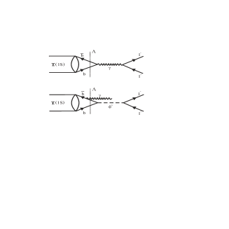
Figure 1: (a)[upper panel]: Electromagnetic annihilation of a $\Upsilon(1S)$ resonance into a charged lepton pair through a virtual photon; (b)[lower panel]: Hypothetical annihilation of a $b\bar{b}{[{}^{1}\!S_{0}^{(1)}]}$ state (existing either as a Fock component of the $\Upsilon$ resonance, or as a consequence of a M1 radiative transition) into a charged lepton pair through a Higgs-like particle (denoted by $\phi^{0}$). The vertical dotted line represents the separation between long-distance physics (on the l.h.s.) and short-distance physics (on the r.h.s.) corresponding to an arbitrary scale $\Lambda$ which can be taken of the order of one hundred MeV, i.e. the soft photon energy.

3.2 Long- and short-distance factorization according to NRET

Instead of supposing a final-state photon radiated by the Upsilon via a M1 transition as in the precedent section, we will now consider the soft $\gamma_{s}$ incorporated as a dynamical photon into a Fock state of the resonance, in analogy to soft gluons in the framework of NRQCD. Admittedly, the strong interaction rules the hadronic dynamics but electromagnetism still has small but observable consequences, e.g. isospin breaking effects [34].

In a naive quark model, quarkonium is treated as a nonrelativistic bound state of a quark-antiquark pair in a static color field which sets up an instantaneous confining potential. Although this picture has been remarkably successful in accounting for the properties and phenomenology of heavy quarkonia, it overlooks gluons whose wavelengths are larger that the bound state size: dynamical gluons permit a meaningful Fock decomposition (in the Coulomb gauge) of physical states beyond the leading non-relativistic description with important consequences both in decays and production of heavy quarkonium.

In particular, the $b\bar{b}$ system in a $\Upsilon$ vector resonance can exist in a configuration other than the dominant $J^{P}=1^{-}$ since the light degrees of freedom mainly formed by gluons and light quark-antiquark pairs can carry the remaining quantum numbers, albeit with a smaller probability. Moreover, it is arguable that soft photons should be included among those low-energy hadronic modes too, therefore allowing the heavy quark-antiquark system to be, for example, in a color-singlet, spin-singlet configuration, i.e. a $|b\bar{b}[{}^{1}\!S_{0}^{(1)}]+\gamma_{s}\rangle$ state . Hence, such dynamical photons would participate in some decay modes of heavy quarkonium, in analogy to dynamical gluons.

According to NRQCD, higher Fock states containing soft gluons indeed can participate actively in the decays of heavy quarkonium, as for example, its annihilation into light hadrons [19, 35]. On the one hand, the probabilities of possible Fock components are encoded in long-distance matrix elements; the heavy quark-antiquark annihilation itself, being a short-distance process, would be perturbatively calculable. On the other hand, details about the complicated nonperturbative hadronization of gluons into final-state light hadrons can be avoided in inclusive channels by assuming the hadronization probability equal to one.

Likewise, one can consider Fock states containing dynamical photons, i.e. pertaining to the hadron during a long-time scale as compared with the short-time process represented in our case by the $b\bar{b}$ annihilation into a dilepton, of order $1/m_{b}$. Thus, a dynamical (quasi-real) photon, stemming from a $|b\bar{b}[{}^{1}\!S_{0}^{(1)}]+\gamma_{s}\rangle$ Fock state, could end up (without need of hadronization) as a final-state photon - though undetected as postulated in this work. Obviously, important differences stand between dynamical gluons and photons so that it will be instructive to review several aspects of NRQCD relevant for our later development.

NRQCD is a low-energy effective theory for the strong interaction removing the unwanted degrees of freedom associated to the heavy quark mass. The following hierarchy between hadronic scales is usually assumed in heavy quarkonium: $m_{Q}\gg m_{Q}\bar{v}\gg m_{Q}\bar{v}^{2}\simeq\ {\Lambda}_{QCD}$, where $m_{Q}$ and $\bar{v}$ denotes the mass and relative velocity of the heavy quark respectively, and $\Lambda_{QCD}$ is the strong interaction scale. The bound state dynamics is chiefly dominated by the exchange of Coulombic gluons with four-momentum $(E\simeq m_{Q}\bar{v}^{2},\vec{p}\simeq m\bar{v})$; soft gluons have four-momenta of order $(m_{Q}\bar{v},m_{Q}\bar{v})$ and ultrasoft gluons of order $(m_{Q}\bar{v}^{2},m_{Q}\bar{v}^{2})$. Likely the above hierarchy makes sense for bottomonium since $\bar{v}^{2}\simeq 10^{-1}$; then the energy of ultrasoft degrees of freedom turns out to be of order $500$ MeV or less. In fact, the separation between energy scales is decisive in phenomenological applications of NRQCD.

Bodwin, Braaten and Lepage [19] showed in a rigorous way that inclusive annihilation decays of heavy quarkonium can be factorized according to soft and hard processes: a) Long-distance physics is encoded in matrix elements, providing the probability for finding the heavy quark and antiquark in a certain configuration within the meson which is suitable for annihilation in each particular case; b) The short-distance annihilation of the $Q\overline{Q}$ pair with given quantum numbers (color, spin, angular momentum and total angular momentum) which could be perturbatively calculated. Therefore, the decay width is written as

$$\Gamma(H)\ =\ \sum_{n}\tilde{\Gamma}_{Q\overline{Q}[n]}(\Lambda)\ \langle H|{\cal O}_{n}^{H}(\Lambda)|H\rangle$$ (12)

where $\Lambda$ is an ultraviolet cutoff of the effective theory, separating the high- and low-energy scales. The short-distance coefficient $\tilde{\Gamma}_{Q\overline{Q}[n]}(\Lambda)$ can be calculated as a perturbation series in $\alpha_{s}(2m_{Q})$. The long-distance parameter $\langle H|{\cal O}_{n}^{H}|H\rangle$ determines the probability for the quarkonium to be in the $[n]$-configuration of the Fock decomposition and can be interpreted as an overlap between the $Q\overline{Q}[n]$ state and the final hadronic state, requiring either a nonperturbative calculation (e.g. on the lattice) or the extraction from experimental data. Similar arguments apply to heavy quarkonium inclusive production (see, for example, [36] and references therein).

In close analogy to the above procedure, let us also introduce an energy parameter $\Lambda$ to separate short- from long-distance physics in the process under study in this work as shown in Fig.1. (One might identify numerically this $\Lambda$ parameter with the upper limit of the integrals (8-10) in the precedent section.) Thus, a factorization of the decay width of the $\Upsilon$ into two pieces is applied: a) the probability ${\cal P}^{\Upsilon}(\eta_{b}^{*}\gamma_{s})$ of the existence within the Upsilon of a $|b\bar{b}[{}^{1}\!S_{0}^{(1)}]+\gamma_{s}\rangle$ Fock state; b) the annihilation width ${\Gamma}_{\eta_{b}^{*}\to\ell\ell}$ into a lepton pair via Higgs boson exchange. Therefore, $\Gamma_{\,\Upsilon\to\gamma_{s}\,\ell\ell}$ can be written in this approach as the product

$$\Gamma_{\,\Upsilon\to\gamma_{s}\,\ell\ell}={\cal P}^{\Upsilon}(\eta_{b}^{*}\gamma_{s})\times{\Gamma}_{\eta_{b}^{*}\to\ell\ell}$$ (13)

This equation follows the spirit of the factorization given in Eq.(12). One important difference, however, is that the long-distance quantity ${\cal P}^{\Upsilon}(\eta_{b}^{*}\gamma_{s})$ can be calculated perturbatively in QED using a quark potential model (for the initial and final state wave functions are involved) because of the smallness of the electromagnetic coupling $\alpha$, in contrast to NRQCD matrix elements. On the other hand, the short-distance parameter ${\Gamma}_{\eta_{b}^{*}\to\ell\ell}$ in Eq.(13) which we may identify with a particular $\tilde{\Gamma}_{Q\overline{Q}[n]}$ coefficient in formula (12), can be calculated with the aid of the Feynman rules of the model under consideration, as we shall later see.

3.2.1 Estimate of the probability ${\cal P}^{\Upsilon}(\eta_{b}^{*}\gamma_{s})$

In NRQCD the probabilities for different Fock configurations of the heavy quark-antiquark pair in heavy quarkonium can be estimated according to the number and order of the chromoelectric and chromomagnetic transitions induced by the interaction effective Lagrangian, needed to reach such states from the lowest configuration or viceversa. Let us point out that in our particular case we are considering a mixed situation where electromagnetic transitions occur between bound states of quarks which are mainly governed by the strong interaction dynamics. Moreover, another caveat is in order: we will compute the transition rate between on-shell states, whereas the pseudoscalar $\eta_{b}^{*}$ state in (13) should be somewhat off-shell. Nevertheless, we will assume this off-shellness small on account of the low energy of the radiated photon.

As commented at the beginning of section 3, we are focusing on the $\Upsilon(1S)$ resonance, mainly because of much more precise experimental data on its tauonic BF as compared to the $\Upsilon(2S)$, as displayed in Table 1, and still missing for the $\Upsilon(3S)$. In addition, the larger number of possible intermediate pseudoscalar bound states for the two latter resonances would make more complicated the theoretical analysis as compared with the $\Upsilon(1S)$ state, where only the lowest $b\bar{b}[{}^{1}\!S_{0}^{(1)}]$ Fock configuration (i.e. a single $\eta_{b}(1S)$ state) should contribute to the final annihilation into a dilepton. Therefore, a textbook expression [32] has been employed to calculate the width corresponding to a transition between S-wave states, i.e. a direct M1-transition between the $\Upsilon(1S)$ and the $\eta_{b}(1S)$ resonances.

The probability of the Fock state $|\eta_{b}^{*}\gamma_{s}\rangle$ $``$inside” a $\Upsilon(1S)$ resonance is then estimated as the ratio,

$${\cal P}^{\Upsilon}(\eta_{b}^{*}\gamma_{s})\ \approx\ \frac{\Gamma^{M1}_{\Upsilon{\rightarrow}\gamma_{s}\eta_{b}}}{\Gamma_{\Upsilon}}\ {\simeq}\ \frac{1}{\Gamma_{\Upsilon}}\ \frac{4\alpha Q_{b}^{2}}{3m_{b}^{2}}\ \Delta E_{hs}^{3}\ \times\ |{\cal M}_{\Upsilon:\eta_{b}}|^{2}\ \sim 10^{-4}$$ (14)

using $m_{b}=M_{\Upsilon}/2\simeq 5$ GeV, and the hyperfine mass splitting between the $\Upsilon$ and $\eta_{b}$ states $\Delta E_{hs}\simeq 50$ MeV as a reference value . The matrix element ${\cal M}_{\Upsilon:\eta_{b}}$ is defined as

$${\cal M}_{\Upsilon:\eta_{b}}=\int_{0}^{\infty}dr\ u_{\Upsilon}(r)\ j_{0}(kr/2)\ u_{\eta_{b}}(r)$$

where $u_{i,f}(r)$ represents the reduced radial wave function of the initial and final resonance respectively, and $j_{0}$ is the spherical Bessel function. We have made in (14) the reasonable approximation: ${\cal M}_{\Upsilon:\eta_{b}}\approx 1$. Let us remark, however, that this parameter involves the wave functions of the $\Upsilon$ and $\eta_{b}$ resonances, actually constituting a nonperturbative matrix element appearing in the long-distance part of the factorized width, in analogy to conventional NRQCD.

In the absence of current experimental data, it is worth noting that the order-of-magnitude $\sim 10^{-4}$ of (14) agrees with more elaborated calculations. For example, Lähde [37] obtains for the partial width of the process $\Upsilon(1S)\rightarrow\eta_{b}(1S)\gamma$ the value 7.7 eV for $\Delta E_{hs}=59$ MeV, which corresponds to a BF of $1.5\times 10^{-4}$ in accordance with (14).

Let us now compare the partial widths of the $\Upsilon(1S)$ decays into three gluons and two gluons plus a photon by means of the ratio [26],

$$r=\frac{\Gamma(\Upsilon(1S)\rightarrow\gamma gg)}{\Gamma(\Upsilon(1S)\rightarrow ggg)}\ \simeq\ \frac{4}{5}\frac{\alpha}{\alpha_{s}}\biggl{(}1-2.6\frac{\alpha_{s}}{\pi}\biggr{)}\ \sim\ 10^{-2}$$ (15)

at the energy scale $\mu^{2}=m_{\Upsilon}^{2}$. Actually, $r$ can be crudely viewed as the relative probability (or suppression factor) of a $|b\bar{b}[{}^{1}\!S_{0}^{(1)}]+\gamma_{s}\rangle$ Fock state w.r.t. the corresponding $|b\bar{b}[{}^{1}\!S_{0}^{(8)}]+g\rangle$ Fock state in the $\Upsilon$ resonance. On the other hand, when the gluon energy is of order $m_{b}\bar{v}^{2}$ or less, the probability for the latter colored Fock state scales as $\bar{v}^{4}$ according to the NRQCD scaling-velocity rules [38, 19]. Thus, numerically ${\cal P}^{\Upsilon}(\eta_{b}^{*}\gamma_{s})\simeq r\times\bar{v}^{4}\sim 10^{-4}$, since $\bar{v}^{2}\simeq 10^{-1}$ for bottomonium, showing the same order-of-magnitude as Eq.(14). Hence, we will assume that Eq.(14) provides a reasonable estimate of the probability for the existence of a $\eta_{b}^{*}$ state within the Upsilon as a function of $\Delta E_{hs}$.

Combining the $``$master” formula (13) and equation (14), the NRET approach leads to

$$\Gamma_{\,\Upsilon\to\gamma_{s}\,\ell\ell}\ =\ \frac{\Gamma^{\,M1}_{\,\Upsilon\to\gamma_{s}\eta_{b}}}{\Gamma_{\Upsilon}}\ \Gamma_{\eta_{b}\to\ell\ell}\ \simeq\ \frac{1}{\Gamma_{\Upsilon}}\frac{16\alpha}{3}\Big{(}\frac{Q_{b}}{2m_{b}}\Big{)}^{2}\Delta E_{hs}^{3}\,\Gamma_{\eta_{b}\to\ell\ell}$$ (16)

for the final decay width, to be compared with Eq.(11) obtained from TOPT.

3.3 Discussion

From Eqs.(11) and (16) it becomes apparent that the calculations of the final width $\Gamma_{\,\Upsilon\to\gamma_{s}\,\ell\ell}$ based upon TOPT or upon factorization à la NRET lead to different results. Indeed, the total width $\Gamma_{\eta_{b}}$ of the $\eta_{b}$ resonance appears in the denominator of formula (11) after the approximations; instead, the total width $\Gamma_{\Upsilon}$ of the $\Upsilon$ resonance appears in formula (16). Since one expects $\Gamma_{\Upsilon}\ll\Gamma_{\eta_{b}}$ , the decay rate for the whole channel $\Upsilon\to\gamma_{s}\,\ell\ell$ stemming from the NRET factorization turns out to be much larger than the decay rate obtained from TOPT. In other words, both approaches are not dual each other.

Actually, the fact that one gets different expressions and hence dissimilar numerical values for the width $\Gamma_{\,\Upsilon\to\gamma_{s}\,\ell\ell}$ in both methods is not contradictory in itself for they are based on distinct physical assumptions. The time-ordered perturbative scheme with $\eta_{b}^{*}$ production above threshold essentially implies a cascade decay, i.e. photon emission and subsequent annihilation of the intermediate hadronic state. Only under this hypothesis and the narrow width approximation, the factorization given by Eq.(11) is justified. On the other hand, the factorization à la NRET postulated in Eq.(16) assumes that a pseudoscalar color-singlet $b\bar{b}$ state exists inside the $\Upsilon$ as a Fock state. Both starting points are different and the results stemming from each framework need not coincide .

In fact, equivalent situations can be found, e.g. in inclusive hadroproduction of heavy quarkonium at large transverse momentum [39], when comparing the color-singlet fragmentation mechanism (where all three perturbative final-state gluons are attached to the hard interaction Feynman diagram) versus the color-octet mechanism (where the emission of two soft gluons from a nonperturbative colored state takes place on a long-time scale). Another example where higher Fock states can compete with perturbative calculations is the explanation given by Braaten and Chen of the long-standing $\rho-\pi$ puzzle of $J/\psi$ and $\psi^{\prime}$ decays [40]. In general, their decays into light hadrons should occur by the annihilation of the $c\bar{c}$ pair into three gluons but the discrepancy with experiment is about two orders of magnitude in this channel. Instead, they argue that the process is dominated by the higher color-octet contribution $c\bar{c}[{}^{3}\!S_{1}^{(8)}]$, thereby annihilating into a light quark pair via $c\bar{c}\to g^{*}\to q\bar{q}$. The suppression of this decay mode for the $\psi^{\prime}$ is attributed to a dynamical effect which cancels the $c\bar{c}$ wavefunction at the origin. (Alternatively, Brodsky and Karliner [41] suggested that the decay into $\rho\pi$ should proceed through the intrinsic charm components of the light mesons.)

Hereafter, we will adopt the NRET factorization as given by the master equation (13) and the numerical estimates will be based on Eq.(16). The low-energy regime of the (ultra)soft photons provides confidence in this approach .

4 Effects of a light neutral Higgs on the leptonic decay width

Following a general scheme, fermions are supposed to couple to the $\phi^{0}$ Higgs field according to a Yukawa interaction term in the effective Lagrangian,

$${\cal L}_{int}^{\bar{f}f}\ =\ -\xi_{f}^{\phi}\ \frac{\phi^{0}}{v}m_{f}\bar{f}(i\gamma_{5})f$$ (17)

where $\xi_{f}^{\phi}$ denotes a factor depending on the type of the Higgs boson and the specific theory under consideration, which could enhance the coupling with a fermion (quark or lepton) of type $``$$f$” and therefore plays a crucial role in our conjecture. In particular, $\phi^{0}$ couples to the final-state leptons proportionally to their masses, ultimately required because of spin-flip in the interaction of a fermion with a (pseudo)scalar, thereby providing an experimental signature for checking the existence of a light Higgs in our study. Lastly, note that the $i\gamma_{5}$ matrix stands only in the case of a pseudoscalar $\phi^{0}$ field.

In this paper we are tentatively assuming that the mass of the light Higgs sought stands close to the $\Upsilon$ resonances below $B\bar{B}$ production: $m_{\phi^{0}}\ {\lesssim}\ 2m_{b}$. As will be argued from current experimental data in the next section, we suppose specifically that $m_{\phi^{0}}$ lies somewhere between the $\Upsilon(1S)$ and $\Upsilon(2S)$ masses, i.e.

$$m_{\Upsilon(1S)}\ {\lesssim}\ m_{\phi^{0}}\ {\lesssim}\ m_{\Upsilon(2S)}$$ (18)

Now, we define the mass difference: ${\Delta}m=|m_{\phi^{0}}-m_{\eta_{b}}|$, where $\eta_{b}$ denotes either a $1S$ or a $2S$ state. Accepting for simplicity that the Higgs boson stands halfway between the mass values of both resonances, we set ${\Delta}m\ {\simeq}\ 0.25$ GeV for an order-of-magnitude calculation.

Hence we write approximately for the scalar tree-level propagator of the $\phi^{0}$ particle in the process (4) entering in the evaluation of $\Gamma_{\eta_{b}\to\ell\ell}$,

$$\frac{1}{(m_{\eta_{b}}^{2}-m_{\phi^{0}}^{2})^{2}+m_{\phi^{0}}^{2}\Gamma_{\phi^{0}}^{2}}\ \simeq\ \frac{1}{(m_{\eta_{b}}^{2}-m_{\phi^{0}}^{2})^{2}}\ \simeq\ \frac{1}{4\ m_{\eta_{b}}^{2}\ ({\Delta}m)^{2}}$$ (19)

where the total width of the Higgs boson $\Gamma_{\phi^{0}}$ has been neglected assuming that $(\Delta m)^{2}\gg\Gamma_{\phi^{0}}^{2}$. We will make a consistency check of this point in subsection 5.1 using numerical values.

Performing a comparison between the widths of both leptonic decay processes (i.e. ${\Gamma}_{\eta_{b}\to\ell\ell}$ versus ${\Gamma}^{(em)}_{\Upsilon\to\ell\ell}$), one concludes with the aid of Eqs.(17-19) and (1) that

$${\Gamma}_{\eta_{b}\to\ell\ell}\simeq\frac{3m_{b}^{4}m_{\ell}^{2}(1-4x_{\ell})^{1/2}|R_{n}(0)|^{2}\xi_{b}^{2}\xi_{\ell}^{2}}{2\pi^{2}(m_{\eta_{b}}^{2}-m_{\phi^{0}}^{2})^{2}v^{4}}\simeq\frac{3\xi_{b}^{2}\xi_{\ell}^{2}}{32\pi^{2}Q_{b}^{2}\alpha^{2}v^{4}}\ \frac{m_{b}^{4}m_{\ell}^{2}}{{\Delta}m^{2}v^{4}}\ \frac{1}{1+2x_{\ell}}{\times}\ {\Gamma}^{(em)}_{\Upsilon\to\ell\ell}$$ (20)

Above we used the non-relativistic approximation (more precisely the static approximation) when assuming null relative momentum of heavy quarks inside quarkonium, and the same wave function at the origin for both the $\Upsilon$ vector state and the $b\bar{b}[{}^{1}\!S_{0}^{(1)}]$ intermediate bound state on account of heavy-quark spin symmetry [19]. Then, the decay amplitude squared of the pseudoscalar state into a $J^{PC}=0^{++}$ (CP-even) Higgs vanishes and only a $0^{-+}$ (CP-odd) Higgs would couple to pseudoscalar quarkonium in this limit. Therefore, the Higgs boson hunted in this way should be properly denoted by $A^{0}$ and, consequently, this notation instead of the generic $\phi^{0}$ will be employed for it from now on.

4.1 Modification of the leptonic BF due to a light CP-odd Higgs contribution

The BF for channel (4) can be readily obtained inserting Eq.(20) into Eq.(16) and afterwards dividing by $\Gamma_{\Upsilon}$, as

$${\cal B}_{\Upsilon{\rightarrow}\gamma_{s}\ell\ell}\ \simeq\ \biggl{[}\frac{\xi_{b}^{2}\xi_{\ell}^{2}m_{b}^{2}m_{\ell}^{2}\,\Delta E_{hs}^{\,3}}{8\pi^{2}{\alpha}(1+2x_{\ell})\Gamma_{\Upsilon}{\Delta}m^{2}v^{4}}\biggr{]}\times{\cal B}_{\ell\ell}$$ (21)

so one can compare the relative rates by means of the following ratio

$${\cal R}=\frac{{\cal B}_{\Upsilon{\rightarrow}\gamma_{s}\ell\ell}}{{\cal B}_{\ell\ell}}\simeq\biggl{[}\frac{\xi_{b}^{2}\xi_{\ell}^{2}m_{b}^{2}\,\Delta E_{hs}^{\,3}}{8\pi^{2}{\alpha}(1+2x_{\ell})\Gamma_{\Upsilon}v^{4}}\biggr{]}\times\frac{m_{\ell}^{2}}{{\Delta}m^{2}}$$ (22)

where we are assuming in the denominator that the main contribution to the leptonic channel comes from the photon-exchange graph of Fig.1(a). Let us point out once again that, since the $\gamma_{s}$ remains undetected, the NP contribution would be experimentally ascribed to the leptonic channel of the $\Upsilon$ resonance. Thus, the ratio (22) represents the fraction of leptonic decays mediated by a CP-odd Higgs, ultimately responsible for the breaking of leptonic universality due to the quadratic mass term $m_{\ell}^{2}$.

Now, to facilitate the comparison of our results with other searches for Higgs bosons, we identify in the following the $\xi_{f}$ factor with the 2HDM (Type II) parameter for the universal down-type fermion coupling to a CP-odd Higgs, i.e. $\xi_{b}=\xi_{\ell}=\tan{\beta}$ [21]. Inserting numerical values into (22) and keeping the leading term in $m_{\ell}^{2}$, one gets the interval

$${\cal R}\ \simeq\ (1.5{\cdot}10^{-7}-1.2{\cdot}10^{-5})\ {\times}\ \tan{}^{4}\beta\ \times\ m_{\ell}^{2}$$ (23)

where use was made of the approximation $m_{A^{0}}\simeq 2m_{b}\simeq 10$ GeV, and the broad range $35-150$ MeV for the possible hyperfine mass diference $\Delta E_{hs}$ [33]; $m_{\ell}$ is expressed in GeV.

Table 1: Measured leptonic BF’s (${\cal B}_{\ell\ell}$) and error bars ($\sigma_{\ell}$) in $\%$, of $\Upsilon(1S)$ and $\Upsilon(2S)$ (from [28]).

channel:	$e^{+}e^{-}$	$\mu^{+}\mu^{-}$	$\tau^{+}\tau^{-}$
$\Upsilon(1S)$	$2.38\pm 0.11$	$2.48\pm 0.06$	$2.67\pm 0.16$
$\Upsilon(2S)$	$1.34\pm 0.20$	$1.31\pm 0.21$	$1.7\pm 1.6$

4.2 Possible $A^{0}-\eta_{b}$ mixing

Long time ago, the authors of references [42, 43] pointed out the possibility of mixing between a light Higgs (either a CP-even or a CP-odd boson) and bottomonium resonances (scalar or pseudoscalar, respectively). Later, Drees and Hikasa [14] made an exhaustive analysis of the phenomenological consequences of the mixing on the properties of both resonances and Higgs bosons. In view of new and forthcoming data on the bottomonium sector from B factories [44, 45], we are particularly interested to apply those ideas looking for experimental signatures to provide an additional check on our conjecture of a light CP-odd Higgs particle.

On the one hand, the mixing can enhance notably the $gg$ decay mode of the Higgs boson [14], ultimately increasing its total decay width. A net effect would be an important decrease of the Higgs tauonic BF (when the $A^{0}$ mass ranges from 9.4 GeV to 11.0 GeV, especially if it lies close to the $\eta_{b}$ masses [14]). An exciting experimental consequence arises in the search for Higgs particles carried out at LEP: higher $\tan{\beta}$ values are allowed than those upper bounds derived from the analysis without considering the mixing [10, 11, 12].

Interestingly, the mixing with a CP-odd Higgs could also modify the properties of the pseudoscalar resonances, i.e. the $\eta_{b}$ states. Thus, even for moderate $\tan{\beta}$ one might expect a disagreement between forthcoming experimental measurements of the hyperfine splitting $m_{\Upsilon}-m_{\eta_{b}}$, and theoretical predictions based on potential models, lattice NRQCD or pQCD [33]. We will come back to this discussion in our numerical analysis of subsection 5.1.

5 Lepton universality breaking?

Let us confront our predictions based on the existence of a CP-odd Higgs boson with experimental results on $\Upsilon$ leptonic decays [28] summarized in Table 1. Indeed, current data show a slight rise of the decay rate with the lepton mass when comparing the $\tau^{+}\tau^{-}$ decay mode with the other two ($e^{+}e^{-}$ and $\mu^{+}\mu^{-}$) modes. However, error bars ($\sigma_{\ell}$) are too large (especially in the $\Upsilon(2S)$ case) to permit a thorough check of the lepton mass dependence as expressed in (23). Nevertheless, we have applied a hypothesis test (see appendix A) to check lepton universality using the $\Upsilon(1S)$ and $\Upsilon(2S)$ data displayed in Table 1.

The null hypothesis (i.e. lepton universality) is compared against the alternative hypothesis stemming from the Higgs contribution predicting a larger (and positive) value of the measured mean of the ${\cal B}_{\ell\ell}$’s differences. Thereby, we conclude that lepton universality can be rejected at a $10\%$ level of significance. As a cornerstone of this work, such slight but measurable variation of the leptonic decay rate (by a ${\cal O}(10)\%$ factor) from the electronic/muonic channel to the tauonic channel can be interpreted theoretically according to the 2HDM upon a reasonable choice of its parameters (e.g. $\tan{\beta}$) as we shall see below.

5.1 Values of $\tan{\beta}$, $A^{0}-\eta_{b}$ mixing and discussion

In order to explain the rise of the tauonic BF by a $\sim 10\%$ factor w.r.t. the electronic/muonic decay modes, one obtains from Eq.(23) that $\tan{\beta}$ should roughly lie over the range:

$$7\ {\lesssim}\ \tan{\beta}\ {\lesssim}\ 21$$ (24)

depending on the value of $\Delta E_{hs}$, namely from 150 MeV down to 35 MeV, whose limits remain somewhat arbitrary however. The partial width for the tauonic decay mode of the $\Upsilon(1S)$ mediated by the CP-odd Higgs turns out to be $\Gamma_{\,\Upsilon\to\gamma_{s}\,\tau\tau}\simeq 140$ eV.

A caveat is in order: the above interval is purely indicative since there are several sources of uncertainty in its calculation, like the actual mass of the hypothetical Higgs and not merely the guess made in Eq.(18) or the crude estimate of the probability ${\cal P}^{\Upsilon}(\eta_{b}^{*}\gamma_{s})$. In fact, higher values of $\tan{\beta}$ were obtained in our earlier work [22] because lower photon energies were used (i.e. between 10 and 50 MeV). Actually, letting ${\cal P}^{\Upsilon}(\eta_{b}^{*}\gamma_{s})$ vary, the range given in Eq.(24) changes accordingly and somewhat higher values cannot be ruled out at all. In sum, our calculations are only approximate and we cannot claim a well-defined interval for $\tan{\beta}$ but just an indication on the values needed to interpret a possible lepton universality breakdown according to our hypothesis . Nevertheless, we perform below a consistency check of (24) concerning several partial widths of the $\eta_{b}$ and $A^{0}$ particles.

Firstly, let us insert the values of $\tan{\beta}$ given by Eq.(24) into Eq.(20) to compute ${\Gamma}_{\eta_{b}\to\tau\tau}$; notice that a high value of $\tan{\beta}$ might yield a large partial width for the $\eta_{b}$ resonance, as compared with the expectation $\Gamma_{\eta_{b}}\simeq 4$ MeV obtained in section 3.1. In fact, using the interval given in (24) one gets ${\Gamma}_{\eta_{b}\to\tau\tau}$ varying from $44$ keV up to 3.56 MeV. Therefore, taking into account the NP contribution to the total decay rate, the Higgs-mediated tauonic BF of the $\eta_{b}$ resonance should stay over the range $0.01\ {\lesssim}\ {\Gamma}_{\eta_{b}\to\tau\tau}/\Gamma_{\eta_{b}}\ {\lesssim}\ 0.5$.

On the other hand, the decay width of a CP-odd Higgs boson into a tauonic or a $c\bar{c}$ pair in the 2HDM(II) can be obtained, respectively, from the expressions: [14]

$$\Gamma(A^{0}\rightarrow\tau^{+}\tau^{-}) \simeq \frac{m_{\tau}^{2}\tan{}^{2}\beta}{8\pi v^{2}}\ m_{A^{0}}\ (1-4x_{\tau})^{1/2}$$ (25)

$$\Gamma(A^{0}\rightarrow c\bar{c}) \simeq \frac{3m_{c}^{2}\cot{}^{2}\beta}{8\pi v^{2}}\ m_{A^{0}}\ (1-4x_{c})^{1/2}$$ (26)

where $x_{\tau}=m_{\tau}^{2}/m_{A^{0}}^{2}$ and $x_{c}=m_{c}^{2}/m_{A^{0}}^{2}$. Below open bottom production, even for moderate $\tan{\beta}$, the $A^{0}$ decay mode would be dominated by the tauonic channel, i.e.

$$\Gamma_{A^{0}}\ \simeq\ \Gamma(A^{0}\rightarrow\tau^{+}\tau^{-})\ \simeq\ 1-10\ MeV$$ (27)

Thus we can confirm the validity of the approximation made in Eq.(19) for the Higgs propagator, i.e. $\Delta m^{2}\gg\Gamma_{A^{0}}^{2}$ (where we tentatively set $\Delta m=250$ MeV).

As commented in subsection 4.2, there is another interesting consequence of our conjecture related to bottomonium spectroscopy due to the mixing between a CP-odd Higgs and $\eta_{b}$ states. (In appendix B we introduce the notation and basic formulae.) Indeed, using the values of $\tan{\beta}$ from Eq.(24) the mixing parameter defined in Eq.(B.2) turns out to be $\delta m^{2}\simeq 1.0-3.1$ GeV². Therefore, such $\eta_{b}-A^{0}$ mixing could induce an observable mass shift of the physical $\eta_{b}$ states which would eventually increase the hyperfine splitting between pseudoscalar and vector resonances w.r.t. a variety of calculations within the SM [33].

Let us now write the masses of the mixed (physical) states as a function of the masses of the unmixed states (marked by a subscript $`$0’, i.e. $\eta_{b0}$ and $A_{0}^{0}$) with the aid of the expression derived from Eq.(B.5) for narrow states and $m_{\eta_{b0}}\simeq m_{A_{0}^{0}}$,

$$m_{\eta_{b},A^{0}}^{2}\ \simeq\ \frac{1}{2}(m_{A_{0}^{0}}^{2}+m_{\eta_{b0}}^{2})\ \pm\ \ \frac{1}{2}[(m_{A_{0}^{0}}^{2}-m_{\eta_{b0}}^{2})^{2}+4(\delta m^{2})^{2}]^{1/2}$$ (28)

Taking as a particular case $\tan{\beta}=16$ ($\delta m^{2}\simeq 2.3$ GeV²), $m_{\eta_{b0}}=9.4$ GeV and $m_{A_{0}^{0}}=9.5$ GeV, we get approximately $m_{\eta_{b}}\simeq 9.32$ GeV and $m_{A^{0}}\simeq 9.58$ GeV, compatible with our tentative hypothesis on the Higgs mass (i.e. ${\Delta}m=|m_{A^{0}}-m_{\eta_{b}}|\simeq 0.25$ GeV) and the experimental mass so far measured for the $\eta_{b}$ meson [33, 28].

6 Summary

In this paper we have interpreted a possible breakdown of lepton universality in $\Upsilon$ leptonic decays (suggested by current experimental data at a $10\%$ level of significance) in terms of a non-standard CP-odd Higgs boson of mass around $10$ GeV, thereby introducing a quadratic dependence on the leptonic mass in the corresponding BF’s. Higher-order corrections within the SM (involving the one-loop $\eta_{b}$ decay into two photons, as estimated in appendix C) fail by far to explain this effect.

The existence of a CP-odd Higgs of mass about 10 GeV mixing with pseudoscalar $b\bar{b}$ resonances should display very clean experimental signatures and therefore could be easily tested with present facilities:

• $``$Apparent” breaking of lepton universality when comparing the BF of the $\tau^{+}\tau^{-}$ decay mode on the one hand, and the BF’s of the electronic and muonic modes on the other. Experimental hints of this possible signature triggered this work [22].

• Presence of monoenergetic photons with energy of order 100 MeV (hence above detection threshold) in those events mediated by the CP-odd Higgs boson (estimated about 10$\%$ of all $\Upsilon$ tauonic decays). This observation would eventually become a convincing evidence of our working hypothesis.

• The $\Upsilon-\eta_{b}$ hyperfine splitting larger than SM expectations, caused by the $A^{0}-\eta_{b}$ mixing. Also a rather large total width of the $\eta_{b}$ resonance due to the NP channel (especially for the higher values of $\tan{\beta}$ shown in (24)).

Although we have focused on a light CP-odd Higgs boson according to a 2HDM(II) for numerical computations, the main conclusions may be extended to other pseudoscalar Higgs-like particles with analogous phenomenological features, as outlined in the Introduction. We thus stress the relevance for checking our conjecture of new measurements of spectroscopy and leptonic decays of the Upsilon family below $B\bar{B}$ threshold in B factories (BaBar [44], Belle[45]) and CLEO [48].

Acknowledgements

I thank G. Bodwin, N. Horwitz, C. Hugonie, M. Krawczyk, F. Martínez-Vidal, P. Ruiz and J. Soto for helpful discussions.

Appendices

Appendix A Lepton universality breaking: hypothesis testing

In Table 2 we show the differences between the branching fractions of the leptonic channels defined as ${\Delta}_{\ell\ell^{\prime}}={\cal B}_{\ell^{\prime}\ell^{\prime}}-{\cal B}_{\ell\ell}$ ($\ell^{\prime},\ell=e,\mu,\tau$) for both $\Upsilon(1S)$ and $\Upsilon(2S)$ resonances, obtained from Table 1 in the main text. Dividing them by their respective experimental errors $\sigma_{\ell\ell^{\prime}}=\sqrt{\sigma_{\ell}^{2}+\sigma_{\ell^{\prime}}^{2}}$ (see also Table 1) one gets the ratios ${\Delta}_{\ell\ell^{\prime}}/\sigma_{\ell\ell^{\prime}}$. Only four of these quantities can be considered as independent. Moreover, in view of the small difference between the electron and the muon masses as compared with the tau mass, we will base our analysis on the comparison between the electron and the muon decay modes on one side, versus the tauonic mode on the other side .

In this analysis, we are especially interested in the alternative hypothesis based on the existence of a light Higgs boson enhancing the decay rate as a growing function of the leptonic squared mass, in opposition to the kinematic factor (2). Therefore, the region of rejection for our statistical test should lie only on one side (or tail) of the ${\Delta}_{\ell\ell^{\prime}}/\sigma_{\ell\ell^{\prime}}$ variable distribution (i.e. positive values if $m_{\ell^{\prime}}>m_{\ell}$), in particular above a preassigned critical value [49, 50]. In other words, we have performed a one-tailed test [49, 50] using the sample consisting of the four independent BF differences between the electronic and the muonic channels versus the tauonic decay mode as explained above (i.e. ${\Delta}_{e\tau}/\sigma_{e\tau}$, ${\Delta}_{\mu\tau}/\sigma_{\mu\tau}$). For the sake of simplicity, we will assume that such differences follow a normal probability distribution with a mean of $0.7775$, obtained from the four ${\Delta}_{\ell\tau}/{\sigma}_{\ell\tau}$ independent values ($\ell=e,\mu$).

Next, let us define the test statistic: $T={\langle}{\Delta}_{\ell\tau}/{\sigma}_{\ell\tau}{\rangle}{\times}\sqrt{N}\simeq 1.555$, where $N=4$ stands for the number of independent points. Indeed note that we are dealing with a Gaussian of unity variance after dividing all differences by their respective errors. Now, we will choose the critical value to be ${\simeq}\ 1.288$ corresponding to a significance level of 10$\%$ in the test. Lepton universality plays the role of the null hypothesis predicting a mean zero (or slightly less), against the alternative (composite) hypothesis stemming from the postulated Higgs contribution predicting a mean value larger than zero . Since experimental data imply that $T>1.288$, we can reject the lepton universality hypothesis at a $10\%$ level of significance . Certainly, this result alone is not statistically significant enough to make any serious claim about the rejection of the lepton universality hypothesis in this particular process, but points out the interest to investigate further the alternative hypothesis stemming from our conjecture on the existence of a light Higgs.

Table 2: All six differences ${\Delta}_{\ell\ell^{\prime}}$ (obtained from Table 1 in the main text) between the leptonic BF’s (in $\%$) of $\Upsilon(1S)$ and $\Upsilon(2S)$ resonances separately. Subscript ${\ell}\ell^{\prime}$ denotes the difference between channels into ${\ell}\bar{\ell}$ and ${\ell}^{\prime}\bar{\ell}^{\prime}$ lepton pairs respectively, i.e. ${\Delta}_{\ell\ell^{\prime}}={\cal B}_{\ell^{\prime}\ell^{\prime}}-{\cal B}_{\ell\ell}$; the ${\sigma}_{\ell\ell^{\prime}}$ values were obtained from Table 1 by summing the error bars in quadrature, i.e. $\sigma_{\ell\ell^{\prime}}=\sqrt{\sigma_{\ell}^{2}+\sigma_{\ell^{\prime}}^{2}}$. Only two ${\Delta}_{\ell\ell^{\prime}}/{\sigma}_{\ell\ell^{\prime}}$ values for each resonance can be considered as truly independent, amounting altogether to a total number of four independent points.

channels	${\Delta}_{\ell\ell^{\prime}}$	$\sigma_{\ell\ell^{\prime}}$	${\Delta}_{\ell\ell^{\prime}}/\sigma_{\ell\ell^{\prime}}$
$\Upsilon(1S)_{e{\mu}}$	$0.1$	$0.125$	$+0.8$
$\Upsilon(1S)_{\mu{\tau}}$	$0.19$	$0.17$	$+1.12$
$\Upsilon(1S)_{e{\tau}}$	$0.29$	$0.19$	$+1.53$
$\Upsilon(2S)_{e{\mu}}$	$-0.03$	$0.29$	$-0.10$
$\Upsilon(2S)_{\mu{\tau}}$	$0.39$	$1.61$	$+0.24$
$\Upsilon(2S)_{e{\tau}}$	$0.36$	$1.61$	$+0.22$

Appendix B Mixing between a CP-odd Higgs and pseudoscalar resonances of bottomonium

The mixing between Higgs and resonances is described by the introduction of off-diagonal elements denoted by $\delta m^{2}$ in the mass matrix. In our case,

$${\cal M}_{0}^{2}\ =\ \left(\begin{array}[]{cc}m_{A_{0}^{0}}^{2}-im_{A_{0}^{0}}\Gamma_{A_{0}^{0}}&\delta m^{2}\\ \delta m^{2}&m_{\eta_{b0}}^{2}-im_{\eta_{b0}}\Gamma_{\eta_{b0}}\end{array}\right)$$ (B.1)

where the subindex $`$0’ indicates unmixed states. The off-diagonal element $\delta m^{2}$ can be computed within the framework of a nonrelativistic quark potential model. For the pseudoscalar case under study, one can write [14]

$$\delta m^{2}\ =\ \xi_{b}\ \biggl{(}\frac{3m_{\eta_{b}}^{3}}{4\pi v^{2}}\biggr{)}^{1/2}|R_{\eta_{b}}(0)|$$ (B.2)

Notice that $\delta m^{2}$ is proportional to $\xi_{b}$, i.e. $\tan{\beta}$ in the 2HDM(II); high values of the latter implies that mixing effects can be important over a large mass region. Substituting numerical values (for the radial wave function at the origin we used the potential model estimate from [51] $|R_{\eta_{b}}(0)|^{2}=$ 6.5 GeV³) one finds (in GeV² units)

$$\delta m^{2}\ \simeq\ 0.146\ \times\ \xi_{b}$$ (B.3)

It is convenient to introduce the complex quantity

$$\Delta^{2}\ =\ \biggl{[}\frac{1}{4}(m_{A_{0}^{0}}^{2}-m_{\eta_{b0}}^{2}-im_{A_{0}^{0}}\Gamma_{A_{0}^{0}}+im_{\eta_{b0}}\Gamma_{\eta_{b0}})^{2}+(\delta m^{2})^{2}\biggr{]}^{1/2}$$ (B.4)

and the mixing quantity $\sin{}2\theta=\delta m^{2}/\Delta^{2}$, where $\theta$ is the (complex) mixing angle of the unmixed $\eta_{b0}$ resonance and $A_{0}^{0}$ Higgs boson giving rise to the physical eigenstates. The masses and decay widths of the mixed (physical) states are thus

$$m_{1,2}^{2}-im_{1,2}\Gamma_{1,2}\ =\ \frac{1}{2}(m_{A_{0}^{0}}^{2}+m_{\eta_{b0}}^{2}-im_{\eta_{b0}}\Gamma_{\eta_{b0}}-im_{A_{0}^{0}}\Gamma_{A_{0}^{0}}\ {\pm}\ \Delta^{2})$$ (B.5)

where subscripts $1,2$ refer to a Higgs-like state and a resonance state respectively, if $m_{A_{0}^{0}}>m_{\eta_{b0}}$; the converse if $m_{A_{0}^{0}}<m_{\eta_{b0}}$.

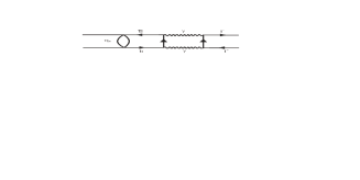
Figure 2: One-loop process within the SM potentially contributing to the dependence of the leptonic BF on the mass of the final-state leptons.

Appendix C $\eta_{b}\rightarrow\ell^{+}\ell^{-}$: one-loop calculation within the Standard Model

In this appendix we consider within the SM an alternative possibility to the Higgs conjecture of a rising leptonic BF of bottomonium with the leptonic mass, based on the electromagnetic decay into a lepton pair of the $\eta_{b}$ state subsequent to the magnetic dipole transition advocated in this work (see Fig.2). Since the width for the $\eta_{b}$ decay into two photons has been recently calculated elsewhere [52], obtaining the range $\Gamma(\eta_{b}\rightarrow\gamma\gamma)\simeq 0.4-0.5$ keV, we can use the following estimate according to the SM:

$$\Gamma_{SM}(\eta_{b}\rightarrow\ell^{+}\ell^{-})\simeq\Gamma(\eta_{b}\ \rightarrow\ \gamma\gamma){\times}\frac{\alpha^{2}m_{\ell}^{2}}{m_{\eta_{b}}^{2}}\frac{1}{2\lambda}\ \biggl{(}\log{\frac{1+\lambda}{1-\lambda}}\biggr{)}^{2}\ll{\Gamma}_{\eta_{b}\to\ell\ell}$$ (C.1)

where $\lambda=(1-4m_{\ell}^{2}/m_{\eta_{b}}^{2})^{1/2}$. The above equation corresponds to the unitary bound due to the absorptive contribution of the two-photon exchange. The last inequality is readily obtained by setting the numerical values for $\tan{\beta}$ used in this work to get $\Gamma_{\eta_{b}\to\ell\ell}$ for any leptonic species.

References

- [1] N. Arkani-Hamed, A.G. Cohen and H. Georgi, Phys. Lett. B513, 232 (2001).
- [2] N. Arkani-Hamed, S. Dimopoulos and G.R. Dvali, Phys. Lett. B429, 263 (1998).
- [3] I. Antoniadis et al., Phys. Lett. B436, 257 (1998).
- [4] L. Randall and R. Sundrum, Phys. Rev. Lett. 83, 3370 (1999).
- [5] T. Han, J.D. Lykken and R-J Zhang, Phys. Rev. D59, 105006-1 (1999).
- [6] G.F. Giudice, R. Rattazzi and J.D. Wells, Nucl. Phys. B595, 250 (2001).
- [7] F. Wilczek, Phys. Rev. Lett. 40, 279 (1978).
- [8] S. Weinberg, Phys. Rev. Lett. 40, 223 (1978).
- [9] U. Schwickerath, hep-ph/0205126.
- [10] Opal Collaboration, Eur. Phys. J. C23, 397 (2002).
- [11] M. Krawczyk et al., Eur. Phys. J. C19, 463 (2001).
- [12] M. Krawczyk, Acta Phys. Polon. B33, 2621 (2002).
- [13] K. Cheung and O.C.W. Kong, hep-ph/0302111.
- [14] M. Drees and K-I Hikasa, Phys. Rev. D41, 1547 (1990).
- [15] H.P. Nilles et al., Phys. Lett. B120, 346 (1983).
- [16] J.R. Ellis et al., Phys. Rev. D39, 844 (1989).
- [17] U. Ellwanger, J.F. Gunion, C. Hugonie and S. Moretti, hep-ph/0305109.
- [18] W.E. Caswell and G.P. Lepage, Phys. Lett. B167, 437 (1986).
- [19] G.T. Bodwin, E. Braaten, G.P. Lepage, Phys. Rev. D51, 1125 (1995).
- [20] F. Wilczek, Phys. Rev. Lett. 39, 1304 (1977).
- [21] J. Gunion et al., The Higgs Hunter’s Guide (Addison-Wesley, 1990).
- [22] M.A. Sanchis-Lozano, Mod. Phys. Lett. A17, 2265 (2002).
- [23] M.A. Sanchis-Lozano, hep-ph/0210364.
- [24] J.F. Gunion, hep-ph/0212150.
- [25] R. Van Royen and V.F. Weisskopf, Nuo. Cim 50, 617 (1967).
- [26] E. Leader and E. Predazzi, An introduction to gauge theories and modern particle physics (Cambridge University Press, 1996).
- [27] CLEO Collaboration, Phys. Lett. B340, 129 (1994).
- [28] Hagiwara et al., Particle Data Group, Phys. Rev. D66,010001 (2002).
- [29] P. Labelle, Phys. Rev. D58,093013 (1998).
- [30] A. Pineda and J. Soto, hep-ph/9707481.
- [31] J.J. Sakurai, Advanced Quantum Mechanics (Addison-Wesley, 1967).
- [32] A. Le Yaouanc et al., Hadron transitions in the quark model (Gordon and Breach Science Publishers, 1988).
- [33] A. Heister et al., Phys. Lett. B530, 56 (2002).
- [34] G. Ecker et al., Nucl. Phys. B591, 419 (2000).
- [35] E. Braaten, hep-ph/9810390.
- [36] J.L. Domenech-Garret and M.A. Sanchis-Lozano, Nucl. Phys. B601, 395 (2001).
- [37] T.A. Lähde, Nucl. Phys. A714, 183 (2003).
- [38] G.A. Schuler, hep-ph/9702230.
- [39] P. Nason et al., hep-ph/0003142.
- [40] Y.-Q. Chen and E. Braaten, Phys. Rev. Lett. 80, 5060 (1998).
- [41] S.J. Brodsky and M. Karliner, Phys. Rev. Lett. 78, 4682 (1997).
- [42] H.E. Haber, G.L. Kane and T.Sterling, Nucl. Phys. B161, 493 (1979).
- [43] J. Ellis et al., Phys. Lett. B83, 339 (1979).
- [44] BaBar Collaboration, Nucl. Instr. Meth. A479, 1 (2002).
- [45] Belle Collaboration, Nucl. Instr. Meth. A479, 117 (2002).
- [46] K. Cheung, C-H Chou and O.C.W. Kong, Phys. Rev. D64, 111301 (2001).
- [47] A. Nyffeler, hep-ph/0305135.
- [48] CLEO Collaboration, hep-ex/0301016.
- [49] A.G. Frodesen et al., Probability ans statistics in particle physics (Universitetsforlaget, 1979).
- [50] B.R. Martin, Statistics for Physicists (Academic Press, London, 1971).
- [51] E. Eichten and C. Quigg, hep-ph/9503356.
- [52] N. Fabiano, hep-ph/0209283.