Particle abundances and spectra in the hydrodynamical description of relativistic nuclear collisions with light projectiles

Abstract

We show that a hydrodynamical model with continuous particle emission instead of sudden freeze out may explain both the observed strange particle and pion abundances and transverse mass spectra for light projectile at SPS energy. We found that the observed enhancement of pion production corresponds, within the context of continuous emission, to the maximal entropy production.

1 Introduction

The main purpose of the ongoing and future heavy ion programs at the high energy laboratories (CERN, BNL) is to investigate the formation and properties of hot dense matter, in particular, the phase transition from hadronic matter to quark gluon plasma (hereafter QGP) predicted by Quantum Chromodynamics (QCD). Various possible signatures of the appearance of the QGP have been suggested: entropy increase (due to the release of new degrees of freedom, namely color), strangeness increase (due to enhanced strange quark production and faster equilibration), $J/\psi$ suppression (due to color screening or collision with hard gluons) or enhancement at higher energy (due to recombination of dissociated $c\bar{c}$ pairs), production of leptons and photons (emitted from a thermalized QGP and unaffected by strong interactions), etc. These signals have been studied extensively in experiments (see for example [1]). More recently, the observed high transverse momentum depletion in Au+Au central collisions at RHIC energies (jet quenching) and also its absence in d+Au collisions, together with the system-size dependence of mono-jet formation, have been considered as a convincing evidence of the formation of QGP at RHIC[2]. On the other hand, some of the above mentioned signals are purely of thermodynamical nature and sometimes their significance is not well defined for finite systems. In such cases, a more careful analysis would be necessary to clarify the effect of finiteness and dynamical evolution of the system on these signals[3]. Some authors suggest that the incident energy dependence of several quantities should be studied and they claim that the set of incident energy dependences of particle multiplicity, average transverse momentum and kaon-pion ratio as a whole indicates the appearance of the mixed phase in central collisions at SPS energies[4]. In fact, if we consider one specific signal of thermodynamical nature, there are many factors which may give a similar response of the claimed signal. For example, it is well known that the hadronic final state interaction also works to suppress $J/\psi$ and the system size dependence should be carefully studied to extract the significance of the observed data. Therefore, it is always important to study and grasp the hadronic effects on other proposed signals.

A major problem to trace back any signature unambiguously to a quark gluon phase is that it is still unknown which theoretical description describes best high energy nuclear collisions. On one extreme, one might use a microscopic model. In principle, such approach would provide a faithful realization of the true physical processes if all the relevant physical degrees of freedom and corresponding interactions were incorporated appropriately. However, in practice, this is not possible and some hypothesis and simplifications are necessarily introduced. For example, we may restrict ourselves to pure hadronic degrees of freedom, but is is known that such models fail[6] to reproduce simultaneously strange and non-strange particle data in nucleon-nucleon collisions and central nucleus-nucleus collisions at SPS energies. Partonic microscopic models are expected to work at energies higher than SPS. One promising approach to describe the final state interactions in heavy ion collisions is the UrQMD model[5]. However, due to the complexity of the calculation and many uncertainties of input data such as hadronic cross sections, it is not easy to get a simple physical insight for the behaviour of the observed quantities.

On the other extreme, one might use a thermal or hydrodynamical model. In such models, it is assumed that a fireball (region filled with dense hadronic matter or QGP in local thermal and chemical equilibrium) is formed in a high energy heavy ion collision and evolves. Hydrodynamical models have been used successfully to describe various kinds of data from AGS to RHIC energies. In particular, at SPS, they are able to account for strangeness data but, in some simplest versions, fail to predict large enough pion abundances (cf. next section). However such an approach has a great advantage compared to the microscopic models in the sense that very few input data are necessary because of the assumption of the local thermal equilibrium. Furthermore, we know that this macroscopic description works quite well suggesting that the local thermal equilibrium in heavy ion collisions is a reasonable approximation. Thus one might ask whether it is possible to introduce a correction to the local thermodynamical equilibrium and its effects on the observed particle abundances. The aim of this paper is to study this problem. We will argue that, within a very simple and natural picture of particle emission (continuous emission), the observed particle abundances and spectra, including strange particles are consistently reproduced. In addition, we show that the non-equilibrium component leads to an increase of entropy of the system, hence a substantial pion increase compared to the usual sudden freezeout mechanism.

2 Hydrodynamical description with (standard) freeze out emission

In the standard hydrodynamical models, one assumes that particle emission, called in this case freeze out, occurs on a sharp three-dimensional surface (defined for example by $T(x,y,z,t)=$ constant). Before crossing it, particles have a hydrodynamical behavior, and after, they free-stream toward the detectors, keeping memory of the conditions (flow, temperature) of where and when they crossed the three dimensional surface. The Cooper-Frye formula [9] gives the invariant momentum distribution in this case

$$Ed^{3}N/dp^{3}=\int_{\sigma}d\sigma_{\mu}p^{\mu}f(x,p).$$ (1)

$d\sigma_{\mu}$ is the surface element 4-vector of the freeze out surface $\sigma$ and $f$ the distribution function of the type of particles considered. This is the formula implicitly used in all standard thermal and hydrodynamical model calculations. It can be integrated to get the particle abundance, which depends only on the freeze out parameters , e.g. $T_{f.out}$.

Freeze out parameters can be extracted by analyzing experimental particle abundances. This has been done by many groups (for a review see e.g. [12]). The models have some variations among them in particular some fit $4\pi$ quantities while others consider quantities in fixed rapidity window, each approach having its own qualities and draw-backs. For a number of these approaches, it was noted that while they can reproduce strange particle abundances, they underpredict the pion abundance. This was first noted by [13] in a study of NA35 data and emphasized by [14, 15] in an analysis of the WA85 strange particle ratios and EMU05 specific net charge $D_{q}\equiv(N^{+}-N^{-})/(N^{+}+N^{-})$ (with $N^{+}$ and N^-, the positive and negative charge multiplicity respectively). A similar problem arises with the Pb+Pb data from NA49 [16, 17].

Various possible improvements have been suggested so that these models could yield both the correct strange particle and pion multiplicities: sequential freeze out [18], hadronic equation of state with excluded volume corrections [19, 20, 17] non-zero pion chemical potential [13, 20, 16], equilibrated plasma undergoing sudden hadronization and immediate decoupling [14, 15, 21], etc. In this paper we follow a different strategy. We feel that the assumption of sudden freeze out on a 3-dimensional surface is a drastic one; in addition it is not sustained by simulations using microscopic models [22]. So we study a different particle emission mechanism, continuous emission.

Before we turn to this, let us note that, to compare particle abundances in the continuous emission and freeze out scenarios, we will use a simplified framework to describe the fluid expansion, namely we suppose longitudinal expansion only and longitudinal boost invariance [23]. This approximation allows to carry out some calculations analytically and turns the physics involved more transparent. It is implicit however that this description applies at best to the midrapidity region and light projectiles (for S+S data, transverse expansion must be small, see e.g. [24]). We should therefore consider midrapidity data such as S+S data from NA35 or WA94, or S+W data from WA85. In fact since we want to consider strange particles and non-strange as well, we will concentrate on NA35 data. In this simplified framework, in the case of a fluid with freeze out at a constant temperature and chemical potential, the Cooper-Frye formula (1) can be re-written ignoring transverse expansion as [25]

$$\frac{dN}{dyp_{\perp}dp_{\perp}}_{\mid y=0}=\frac{gR^{2}}{2\pi}\tau_{f.out}(T_{f.out},T_{0},\tau_{0})m_{\perp}\sum_{n=1}^{\infty}(\mp)^{n+1}\exp(\frac{n\mu_{f.out}}{T_{f.out}})K_{1}(\frac{nm_{\perp}}{T_{f.out}})$$ (2)

(The plus sign corresponds to bosons and minus, to fermions.) It depends on the conditions at freeze out: $T_{f.out}$ and $\mu_{f.out}=\mu_{b\,f.out}B+\mu_{S\,f.out}S$, with B and S the baryon number and strangeness of the hadron species considered, and $\mu_{S\,f.out}(\mu_{b\,f.out},T_{f.out})$ obtained by imposing strangeness neutrality. So the experimental spectra of particles teach us in that case what the conditions were at freeze out.

3 Hydrodynamical description with continuous emission

The notion that particle emission does not necessarily occur on a three dimensional surface but may be continuous was incorporated in a hydrodynamical description in [26]. In this model, the fluid is assumed to have two components, a free part plus an interacting part and its distribution function reads

$$f(x,p)=f_{free}(x,p)+f_{int}(x,p).$$ (3)

$f_{free}$ counts all the particles that last scattered earlier at some point and are at time $x^{0}$ in $\vec{x}$. $f_{int}$ describes all the particles that are still interacting (i.e. that will suffer collisions at time $>x^{0}$). The invariant momentum distribution is then

$$Ed^{3}N/dp^{3}=\int d^{4}x\,D_{\mu}[p^{\mu}f_{free}(x,p)].$$ (4)

$D_{\mu}[p^{\mu}f_{free}(x,p)]$ is a covariant divergence in general coordinates and $d^{4}x$ is the invariant volume element. A priori formula (4) is sensitive to the whole fluid history and not just to freeze out conditions as in formula (1).

In the simplified framework that we will use to compare particle abundances in the continuous emission and freeze out scenarios, we can approximate the equation of continuous emission (4) as [26]

$$\frac{dN}{dyp_{\perp}dp_{\perp}}_{\mid y=0}\sim\frac{2g}{(2\pi)^{2}}\int_{{\cal P}=0.5}d\phi d\eta\frac{m_{\perp}\cosh\eta\tau_{F}\rho d\rho+p_{\perp}\cos\phi\rho_{F}\tau d\tau}{\exp((m_{\perp}\cosh\eta-\mu)/T)\pm 1}$$ (5)

where ${\cal P}$ is the probability to escape without collision calculated with a Glauber formula, $\tau_{F}$ and $\rho_{F}$ are respectively solution of ${\cal P}(\tau_{F},\rho,\phi,\eta;v_{\perp})=0.5$ and ${\cal P}(\tau,\rho_{F},\phi,\eta;v_{\perp})=0.5$ where $v_{\perp}$ is the particle transverse velocity. In (5), various $T$ and $\mu=\mu_{b}B+\mu_{S}S$ appear ($\mu_{S}$ is obtained from strangeness neutrality), reflecting the whole fluid history, not just $T_{f.out}$ and $\mu_{b\,f.out}$. This history is known by solving the hydrodynamical equations of a hadronic gas with continuous emission; it depends only on the initial conditions $T_{0}$ and $\mu_{b0}$ at the initial time $\tau_{0}$ (we use the standard value $\tau_{0}=1\,fm$). Therefore (5) only depends on the initial conditions. We expect that heavy particles, due to thermal suppression, will bring information on early times when they are more numerous. Fast particles can escape more easily from dense matter, so they will probe early times, whereas slow particles will probe late times, when they are finally in diluted matter and make their last collision. Light particles such as the pion should probe the whole fluid history.

4 Results for continuous emission

In [27], we showed that it is possible to find initial conditions for the hydrodynamical evolution of the fluid that leads to WA85 strange particle ratios. In this paper, we want to broader this study. First we want to show that not just ratios, but abundances can be reproduced for a certain set of initial conditions. This is not trivial: for freeze out, fitting abundances or ratios is not very different because of volume cancellation, but not for the continuous emission which is a process sensitive to the whole fluid history, particle mass and particle velocity. Second, we want to check that for the same initial conditions that reproduce abundances, spectra can be reproduced.

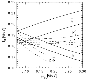
Figure 1: Allowed region for the initial conditions determined from the NA35 S+S midrapidity data.

Abundances can be obtained by integrating (5). Figure 1 shows the allowed region of initial conditions that lead to the experimental NA35 $y=0$ values [28] $\Lambda=1.26\pm 0.22_{p_{\perp}>0.5GeV}$, $\overline{\Lambda}=0.44\pm 0.16_{p_{\perp}>0.5GeV}$, $K_{S}^{0}=1.30\pm 0.22_{p_{\perp}>0.62GeV}$, $h^{-}=26\pm 1$ and $p-\overline{p}=3.2\pm 1.0$. We do not use the $K^{+}$ and $K^{-}$ abundances because they were measured outside the mid-rapidity region. Considering only strange particles, the allowed window is $T_{0}\sim 183-188$ MeV, $\mu_{b0}\sim 70-125$ MeV, with an ideal hadron gas equation of state and the strangeness saturation factor (a multiplicative factor for (5)) $\gamma_{s}=1.3$. Including the $p-\bar{p}$ abundance decreases the window for $\mu_{b0}$ to $\sim 70-105$ MeV. Finally including the abundance of negative particles leads to the small window $T_{0}\sim 185$ MeV and $\mu_{b0}\sim 100$ MeV.

Using a more sofisticated equation of state, the value of $T_{0}$ might be decreased [27] by some 10-15 % i.e. to 155-165 MeV, compatible with (i.e. below) QCD lattice values for the phase transition temperature from QGP to hadronic matter. Our value of $\gamma_{S}$ is above 1 and this might look surprising. However, its value is decreased by some 15 % when looking at a more realistic equation of state. In addition, we have imposed strangeness neutrality, it is possible that this is a too strong constraint when analyzing data taken in a very restricted rapidity region (see [29] where a similar problem was encountered). Note that using a larger value of $\gamma_{s}$, the size of the allowed window for initial conditions in figure 1 increases. Aside of the uncertainty in the equation of state, there are other factors that influence the precise location and size of the window but few: value of the cross section, $=2\,fm^{2}$, (taken constant for simplicity here) in the Glauber formula, value of the cutoff ${\cal P}=0.5$ which in fact is equivalent to a change in the cross section [26], and value of the initial time for the hydrodynamical evolution for which the canonical value of $\tau_{0}=1\,fm$ was assumed.

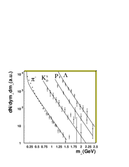
Figure 2: Transverse mass spectrum computed for the initial conditions obtained in figure 1 and comparison with NA35 (all-y) data. No decays included.

With the initial conditions determined by figure 1, particle spectra can be computed and compared with (all rapidity) NA35 data. This is shown in figure 2. The agreement is reasonable. No decays have been included, this should in particular lead to an improvement of the low $m_{\perp}$ pion spectrum.

Therefore there exist initial conditions of the hydrodynamical expansion such that NA35 strange and non-strange particle abundances and spectra can be reproduced simultaneously without extra assumption, in contrast to some of the freeze out models mentioned above. In fact it is puzzling that the continuous model leads to so many more pions than the freeze out model and it is necessary to investigate the reason.

To illustrate more precisely the difference between (simple) freeze out and continuous emission scenarios, we compare in table 1 results from both scenarios, with $T_{0}=185MeV$ and $\mu_{b0}=100MeV$ for the continuous emission case, $T_{f.out}=185MeV$ and $\mu_{b\,f.out}=100MeV$ for the freeze out case (with the scaling factor $\tau_{f.out}$ in (2) taken equal to $1\,fm$) . For both cases, we assume that initially the matter is a hadron gas and $\gamma_{s}=1.3$. Heavy particles, in the continuous emission case, due to thermal suppression, are mostly emitted early [27], i.e. in similar conditions than in the freeze out model in the case $\mu_{b\,0}=0$ and for some longer time if $\mu_{b\,0}\neq 0$. Pions in the freeze out case are too few as discussed previously: 15.7 instead of $26\pm 1$. Pions in the continuous emission case, on the other side, are emitted early and then on, and we get substantially more of them, 27 in agreement with data.

In a hydrodynamical model without shocks and dissipation, entropy is conserved. In the usual freeze out scenario, this is an important point because the initial entropy can be determined from the final multiplicity. To illustrate this connection, let us consider a thermalized massless pion fluid. In this case, the entropy density is related to the pion density at all temperature by $s=3.6n_{\pi}$. Therefore knowing the pion number at freeze out (from data) $N_{\pi}^{f.out}$, one can infer the entropy at freeze out $S^{f.out}$ and the initial value of the entropy

$$S_{0}=S^{f.out}=3.6N_{\pi}^{f.out}$$ (6)

(since entropy is conserved).

In the continuous emission case, we can compute the number of free particles in principle from (4)

$$N_{\pi}^{free} = \int d^{4}x\int d^{3}pD_{\mu}(\frac{p^{\mu}}{E}f_{free})$$

$$= \int d^{4}xD_{\mu}\left[\frac{g}{(2\pi)^{3}}\int d^{3}p\frac{p^{\mu}}{E}\frac{1}{e^{(u.p)/T}-1}\frac{\cal P}{1-{\cal P}}\right]$$

$$= \int d^{4}xa(x)n_{th}^{m=0}(x)$$

where we used the factorization property arising from the zero mass assumption [26]) and introduced a kind of weight, $a(x)\equiv D_{\mu}(A^{\mu}n_{th}^{m=0})/n_{th}^{m=0}$ with $A^{\mu}=(\int d\Omega/(4\pi)\,{\cal P}/(1-{\cal P}),\int d\Omega\sin\theta\cos\phi/(4\pi)\,{\cal P}/(1-{\cal P}),\int d\Omega\sin\theta\sin\phi/(4\pi)\,{\cal P}/(1-{\cal P}),\int d\Omega\cos\theta/(4\pi)\,{\cal P}/(1-{\cal P}))$.

We re-write (7) by assuming that the fluid is divided in small volumes $V_{\alpha}(\tau)$ moving with it and time is discretized with $\tau_{i+1}=\tau_{i}+\Delta\tau$, so

$$N_{\pi}^{free}=\sum_{\alpha=1}^{\infty}\sum_{i=1}^{\infty}\Delta\tau\Delta V_{\alpha}(\tau_{i})a(\tau_{i})n_{th}^{m=0}(\tau_{i})$$ (8)

At time $\tau_{i}$, $\Delta V_{\alpha}(\tau_{i})$ contains a mixture of free plus thermalized particles and we suppose that the thermalized pions break into those which have just done their last collisions (joining the free component of the fluid) and those which remain interacting. This interacting component is supposed to have reached thermal equilibrium at $\tau_{i+1}$ and the process of separation between free and interacting part repeats itself. We note that both the separation (free/interacting) process and the re-thermalization one (even if incomplete) lead to entropy increase, which can manifests itself as pions. Exactly how much entropy is created and how much appears as pions is model-dependent, but this effect should always be present. Depending on the process involved, this can be a substantial effect. Indeed as shown in table 1 and discussed above, in the particular case of continuous emission with $f_{int}\sim f_{th}$ (complete rethermalization), the amount of extra pions can even reach 70%. It would be worth checking if this is the case with the improved description of continuous emission [30]. The hypothesis $f_{int}\sim f_{th}$ corresponds to the upper limit of entropy production. It is interesting to note that the observed pion abundance is reproduced just by the maximal entropy production within the present mechanism. Comparing results from UrQMD and the thermal statistical model [5], it was shown that the entropy density per baryon density increases by 15 % with increasing times, or alternatively for temperatures decreasing from 161 to 126 MeV, in a central cell $5\times 5\times 5fm^{3}$ for Pb+Pb at SPS. In our case, for such a central cell, away from the border, we have initially little continuous emission and the entropy per baryon increases slowly. The large increase of pion abundance obtained above occurs in the space-time domain where continuous emission becomes considerable.

5 Conclusion

In this paper, we discussed data on strange and non-strange particles at ultrarelativistic energy with light projectiles, from a hydrodynamical point of view. Some versions of the standard model with sudden freeze out can reproduce the strange particle data but underpredicts the pion abundance, if no extra assumption is made. In addition, it is usually necessary to assume two different freezeouts, chemical and thermal, to account for both strange particle abundances and particle transverse mass spectra. We showed that a hydrodynamical model with a more precise emission process, continuous emission, can reproduce both the strange and non-strange particle abundances without extra assumption in addition to being consistent with other types of experimental data such as transverse mass spectra. In the two freeze outs case, typical parameters are chemical freeze out temperature, baryonic potential and strangeness saturation factor as well as thermal freeze out temperature and baryonic potential; they are fixed by data. In the continuous emission, the parameters are: the initial conditions $T_{0}$, $\mu_{b0}$ and $\gamma_{s}$, which are fixed by data; the average interacting cross section and initial time were chosen to have the canonical values $2\,fm^{2}$ and $1\,fm$. We note that while in freeze out models, data give information only on the freeze out conditions, in continuous emission, observables depend on the whole fluid history. Therefore what observables teach us depend on the emission model. This point is reinforced by a comparison of Bose-Einstein correlations for freeze out and continuous emission [31]

Our main point is the following: in the usual freeze out scenario, a large pion number may be associated with a large entropy (cf. (6)). Here we showed that a large pion number can be generated by continuous emission. The reason for this increase is entropy generation during the separation and rethermalization processes occurring during continuous emission. We stressed that how large is this increase is model-dependent, but in any case this possibility sheds a new light on the problem of pion emission at SPS. For freeze out, a large experimental value of $N_{\pi}$ implies a large initial entropy $S_{0}$ and may be considered a hint of QGP formation (see e.g. [14, 15]). For continuous emission, a large pion number and entropy may be a natural outcome independently of QGP formation. Consequently, a better understanding of particle emission in the hydrodynamical regime is necessary to assess the possibility of QGP formation in relativistic heavy ion collisions.

References

Table 1: Comparison of experimental particle abundances with continuous emission and freeze out predictions for S+S collisions at midrapidity.

• 	experimental value	continuous emission	freeze out
  $\Lambda$	1.26$\pm$0.22	0.96	0.92
  $\bar{\Lambda}$	0.44$\pm$0.16	0.29	0.46
  $p-\bar{p}$	3.2$\pm$1.0	3.12	1.32
  $h^{-}$	26$\pm$1	27	15.7
  $K^{0}_{S}$	1.3$\pm$0.22	1.23	1.06

References

- [1] Harris J W and Müller B 1996 Ann. Rev. Nucl. Part. Sc. 46 71
- [2] Adler S S et al. nucl-ex/0306021 Adams J et al. nucl-ex/0306024; Back B B et al. nucl-ex/0306025; Gyulassy M Talk at the 8th International Wigner Symposium
- [3] Stöcker et al. 2002 AIP Conference Proceedings vol 631 p 553
- [4] Gazdzicki M and Gorenstein M I 1999 Acta Phys. Polon. B30 2705 Gazdzicki M et al. hep-ph0303041 Gazdzicki M hep-ph/0305176
- [5] Bravina L V et al. 1999 Phys. Rev. C 60 024904
- [6] Odyniec G J 1998 Nucl. Phys. A 638 135c
- [7] Müller B 1999 Nucl. Phys. A 661 272c Antinori F et al. 1999 Nucl. Phys. A 661 130c
- [8] Geiger K 1998 Nucl. Phys. A 638 551c
- [9] Cooper F and Frye G 1974 Phys. Rev. D 10 186
- [10] Arbex N, Grassi F, Hama Y and Socolowski Jr. O 2001 Phys. Rev. C 64 064906
- [11] Broniowski W and Florkowski W 2001 Phys. Rev. Lett. 87 272302.
- [12] Cleymans J and Redlich K 1999 Phys. Rev. C 60 054908 Braun-Munzinger P et al. nucl-th/0304013
- [13] Davidson N J et al. 1992 Z. Phys. C 56 319
- [14] Letessier J et al. 1993 Phys. Rev. Lett. 70 3530.
- [15] Letessier J et al. 1995 Phys. Rev. D 51 3408
- [16] Tomášik B, Wiedemann U A and Heinz U nucl-th/9907096
- [17] Yen G D and Gorenstein M I 1999 Phys.Rev.C 59 2788
- [18] Cleymans J et al. 1993 Z. Phys. C 58 347
- [19] Ritchie R A et al. 1997 Z. Phys. C 75 535
- [20] Yen G D et al. 1997 Phys. Rev. C 56 2210
- [21] Letessier J and Rafelski J 1999 Phys. Rev. C 59 947
- [22] Bravina L et al. 1995 Phys. Lett. B 354 196 Bravina L et al. 1999 Phys. Rev. C 60 044905 Sorge H 1996 Phys. Lett. B 373 16 S.Bass et al. 1999 Phys. Rev. C 60 021902
- [23] Hwa R C 1974 Phys. Rev. D 10 2260 Chiu C B and Wang K H 1975 Phys. Rev. D 12 272 Sudarchan E C and Wang K H 1975 Phys. Rev. D 12 902 Bjorken J D 1983 Phys. Rev. D 27 140
- [24] Schnedermann E et al. 1993 Phys. Rev. C 48 2462 Schnedermann E et al. 1994 Phys. Rev. C 50 1675
- [25] Ruuskanen P V 1987 Acta Physica Polonica B 18 551
- [26] Grassi F, Hama Y and Kodama T 1995 Phys. Lett. B 355 9 Grassi F, Hama Y and Kodama T 1996 Z. Phys. C 73 153
- [27] Grassi F and Socolowski Jr. O 1998 Phys. Rev. Lett. 80 1170
- [28] Bartke J et al. 1990 Z. Phys. C 48 191 Bartke J et al. 1993 Z. Phys. C 58 367 Bartke J et al. 1994 Z. Phys. C 64 195 Bartke J et al. 1994 Phys. Rev. Lett. 72 1419
- [29] Sollfrank J et al. 1994 Z. Phys. C 61 659
- [30] Sinyukov Yu M, Akkelin S V and Hama Y 2002 Phys. Rev. Lett. 89 052301
- [31] Grassi F, Hama Y, Padula S and Socolowski Jr. O 2000 Phys. Rev. C 62 044904
-