IPPP/03/37

DCPT/03/74

23rd July 2003

Hadronic Radiation Patterns in
Vector Boson Fusion Higgs Production

V. A. Khoze, W. J. Stirling and P. H. Williams

Institute for Particle Physics Phenomenology

University of Durham

Durham, DH1 3LE, U.K.

We consider the hadronic radiation patterns for the generic process of $b\bar{b}+2\;$forward jet production at the LHC, where the (centrally produced) $b\bar{b}$ originate either from a Higgs, a $Z$ or from standard QCD production processes. A numerical technique for evaluating the radiation patterns for non-trivial final states is introduced and shown to agree with the standard analytic results for more simple processes. Significant differences between the radiation patterns for the Higgs signal and the background processes are observed and quantified. This suggests that hadronic radiation patterns could be used as an additional diagnostic tool in Higgs searches in this channel at the LHC.

1 Introduction

The distribution of soft hadrons or jets accompanying energetic final–state particles in hard scattering processes is governed by the underlying colour dynamics at short distances [1, 2, 3, 4]. The soft hadrons paint the colour portrait of the parton hard scattering, and can therefore act as a ‘partonometer’ [1, 2, 3, 4, 5, 6, 7, 8, 9, 10, 11, 12]. Since signal and background processes at hadron colliders can have very different colour structures (compare for example the $s$–channel colour singlet process $gg\to H\to b\bar{b}$ with the colour octet process $q\bar{q}\to g^{*}\to b\bar{b}$), the distribution of accompanying soft hadronic radiation in the events can provide a useful additional diagnostic tool for identifying new physics processes.

Examples that have been studied in the literature in this way include Higgs [13], $Z^{\prime}$ [9] and leptoquark [14] production. In each case the new particle production process was shown to have its own particular colour footprint, distinctively different from the corresponding background process.

Quite remarkably, because of the property of Local Parton Hadron Duality (see for example Refs. [2, 3, 15]) the distribution of soft hadrons can be well described by the amplitudes for producing a single additional soft gluon. The angular distribution of soft particles typically takes the form of an ‘antenna pattern’ multiplying the leading–order hard scattering matrix element squared. Confirmation of the validity of this approach comes from studies of the production of soft hadrons and jets accompanying large $E_{T}$ jet and $W+$jet production by the CDF [16] and D0 collaborations [17] at the Fermilab Tevatron.

One of the most important physics goals of the CERN LHC $pp$ collider is the discovery of the Higgs boson. Many scenarios, corresponding to different production and decay channels, have been investigated, see for example the studies reported in Refs. [18, 19, 20]. In a recent paper [21], we have studied Higgs production via vector boson fusion at the LHC, $qq\to qqH$, where the colour–singlet nature of the $V^{*}V^{*}\to H$ production process naturally gives rise to rapidity gaps between the centrally produced Higgs and the forward jets. The most delicate issue in calculating the cross section for processes with these rapidity gaps concerns the soft survival factor $\hat{S}^{2}$. This non-universal factor has been calculated in a number of models for various rapidity gap processes, see for example [22] and references therein. Although there is reasonable agreement between these model expectations, it is always difficult to guarantee the precision of predictions which rely on soft physics. However, in [21] we argued that the calculations of $\hat{S}^{2}$ can be checked experimentally by computing and measuring the event rate for a suitable calibrating process, for example the production of a $Z$ boson with the same rapidity gap and jet configuration as for the (comparatively light) Higgs, see also [28].

In this paper we adopt a different approach to the same problem. Rather than considering the case where the emission of soft hadrons between the jets and central Higgs is suppressed (rapidity gaps), we instead discuss the inclusive distribution using the antenna pattern approach to quantify the relative amounts of soft hadron emission in the signal and background events. In other words, we quantify how ‘quiet’ the signal events are compared to the otherwise irreducible background events.

Thus we have in mind the following type of scenario. Suppose an invariant mass peak is observed in a sample of (tagged) $b\bar{b}$ events in which there are energetic forward jets, typical of the vector–boson production process. If such events do indeed correspond to Higgs production, then the distribution of accompanying soft radiation in the event — which we take to mean the angular distribution of hadrons or ‘minijets’ with energies of at most a few GeV, well separated from the beam and final–state energetic jet directions — will look very different from that expected in background QCD production of $b\bar{b}+2\;$jet events. Again, the analogous process of $Z(\to b\bar{b})+2\;$jet production can be used to calibrate the analysis, since these events are, as we shall see, also generally quieter than the QCD backgrounds.

Thus in this study we will consider the hadronic radiation patterns for the generic process of $b\bar{b}+2\;$forward jet production, where the (central) $b\bar{b}$ originate either from a Higgs, a $Z$ or from standard QCD production processes. We will chose configurations (i.e. cuts on the rapidities and tranvserse momenta of the final–state particles) that maximise the Higgs signal to background ratio, see [21].

The paper is organised as follows. In the following section we consider the antenna patterns for Higgs and $Z$ production accompanied by two forward jets. We show that for these colour—singlet production processes, fairly simple analytic expressions can be derived. However this is not the case for the more complicated QCD background processes. In Section 3 we show that the radiation patterns for these can be calculated using a more general numerical technique, which indeed can be applied to arbitrarily complicated processes. Section 4 summarises our results and presents our conclusions.

2 Hadronic Antenna Patterns for Higgs and $Z+2$ Jet Production

2.1 Higgs and Electroweak $Z$ Production

The signal process we are interested in is Higgs production via vector boson fusion, shown in Fig. 1, with subsequent decay of the Higgs to $b\bar{b}$.

Figure 1: Higgs production via electroweak vector boson fusion.

Furthermore, we restrict our considerations to the case where the outgoing quark jets are forward in rapidity and the Higgs decay products are central in the detector. Throughout this paper, we work in the zero width approximation for the Higgs and $Z$. As vector boson fusion involves no colour flow in the $t$-channel, the radiation pattern is simply that of the $2\rightarrow 2$ process $qq^{\prime}\rightarrow qq^{\prime}$, with an additional colour disconnected $b\bar{b}$. These were calculated in [9]. Note also that we work with massless quarks. The radiation pattern is defined as the ratio of the $2\rightarrow n+1$ and $2\rightarrow n$ matrix elements using the soft gluon approximation in the former. The dependence on the soft gluon momentum $k$ then enters via the eikonal factors (‘antennae’) [1, 3]

$$[ij]\equiv\frac{p_{i}\cdot p_{j}}{(p_{i}\cdot k)(p_{j}\cdot k)}.$$ (2.1)

For the signal $q(p_{1})\,q^{\prime}(p_{2})\rightarrow q(p_{3})\,q^{\prime}(p_{4})+g(k)$ we have

$$\overline{\sum}|\mathcal{M}|^{2}=\frac{g_{s}^{6}C_{F}}{N_{c}}\left(\frac{s^{2}+u^{2}}{t^{2}}\right)2C_{F}([13]+[24])$$ (2.2)

with $s\equiv(p_{1}+p_{2})^{2}$, $t\equiv(p_{1}-p_{3})^{2}$, $u\equiv(p_{1}-p_{4})^{2}$.

We then normalise this by the matrix element for the leading order process $q(p_{1})\,q^{\prime}(p_{2})\rightarrow q(p_{3})\,q^{\prime}(p_{4})$:

$$\overline{\sum}|\mathcal{M}|^{2}=\frac{g_{s}^{4}C_{F}}{N_{c}}\left(\frac{s^{2}+u^{2}}{t^{2}}\right).$$ (2.3)

Note that in this particular case, the $2\rightarrow 3$ matrix element in the soft gluon limit factorises into the form $(2\rightarrow n\textrm{ matrix element})\times(\textrm{antenna factor})$. This feature is not universal, being restricted to only very simple cases such as this. The antenna pattern is then

$$\mathcal{R}(qq^{\prime}\rightarrow qq^{\prime})=g_{s}^{-2}\frac{|\overline{\mathcal{M}}_{3}|^{2}(qq^{\prime}\rightarrow qq^{\prime}+g)}{|\overline{\mathcal{M}}_{2}|^{2}(qq^{\prime}\rightarrow qq^{\prime})}=2C_{F}([13]+[24]).$$ (2.4)

As we are working in the zero width approximation we can include the decay of the Higgs into (massless) $b\bar{b}$ by simply adding the antenna for this colour disconnected part. The hadronic radiation pattern for $q(p_{1})\,q^{\prime}(p_{2})\,\rightarrow q(p_{3})\,q^{\prime}(p_{4})\,H\;;\;H\rightarrow b(p_{5})\,\bar{b}(p_{6})$ is then

$$\mathcal{R}(H)=2C_{F}([13]+[24]+[56]).$$ (2.5)

In order to visualise the pattern we must specify the kinematics and pick a relevant configuration for the incoming and outgoing particles. We label the four-momenta by

$$a(p_{1})+b(p_{2})\rightarrow c(p_{3})+d(p_{4})+\cdots+g(k),$$ (2.6)

where the gluon is soft relative to the other large-$E_{T}$ final state partons, i.e. $k\ll E_{T}$. We ignore the gluon momentum in the energy-momentum constraints, work in the overall parton centre of momentum frame, fix the Higgs to be at rest in that frame and its decay products at $(\eta_{\textrm{b}},\phi_{\textrm{b}})=(0,\pi/2)$ and $(0,3\pi/2)$. With the notation $p^{\mu}=(E,p_{x},p_{y},p_{z})$, the momenta are then

$$p_{1}^{\mu} = (m_{H}/2+E_{T}\cosh\eta_{\textrm{jet}},0,0,m_{H}/2+E_{T}\cosh\eta_{\textrm{jet}}),$$

$$p_{2}^{\mu} = (m_{H}/2+E_{T}\cosh\eta_{\textrm{jet}},0,0,-m_{H}/2-E_{T}\cosh\eta_{\textrm{jet}}),$$

$$p_{3}^{\mu} = (E_{T}\cosh\eta_{\textrm{jet}},0,E_{T},E_{T}\sinh\eta_{\textrm{jet}}),$$

$$p_{4}^{\mu} = (E_{T}\cosh\eta_{\textrm{jet}},0,-E_{T},-E_{T}\sinh\eta_{\textrm{jet}}),$$

$$p_{H}^{\mu} = (m_{H},0,0,0),$$

$$p_{b}^{\mu} = (m_{H}/2,m_{H}/2,0,0),$$

$$p_{\bar{b}}^{\mu} = (m_{H}/2,-m_{H}/2,0,0),$$

$$k^{\mu} = (k_{T}\cosh\eta_{\textrm{g}},k_{T}\sin\phi_{\textrm{g}},k_{T}\cos\phi_{\textrm{g}},k_{T}\sinh\eta_{\textrm{g}}).$$ (2.7)

This is the appropriate form for studying the angular distribution of the soft gluon, parametrised by $\eta_{\textrm{g}}$ and $\phi_{\textrm{g}}$. Using the kinematics of Eq. (2.1) with Eq. (2.5) gives

$$\mathcal{R}(H) = \frac{2C_{F}}{k_{T}^{2}}\left\{\frac{\cosh\eta_{\textrm{jet}}-\sinh\eta_{\textrm{jet}}}{(\cosh\eta_{\textrm{g}}-\sinh\eta_{\textrm{g}})(\cosh\eta_{\textrm{jet}}\cosh\eta_{\textrm{g}}-\cos\phi_{\textrm{g}}-\sinh\eta_{\textrm{jet}}\sinh\eta_{\textrm{g}})}\right.$$ (2.8)

$$+ \frac{\cosh\eta_{\textrm{jet}}-\sinh\eta_{\textrm{jet}}}{(\cosh\eta_{\textrm{g}}+\sinh\eta_{\textrm{g}})(\cosh\eta_{\textrm{jet}}\cosh\eta_{\textrm{g}}+\cos\phi_{\textrm{g}}+\sinh\eta_{\textrm{jet}}\sinh\eta_{\textrm{g}})}$$

$$+ \left.\frac{2}{(\cosh\eta_{\textrm{g}}-\sin(\phi_{\textrm{g}}+\pi))(\cosh\eta_{\textrm{g}}+\sin(\phi_{\textrm{g}}+\pi))}\right\}$$

Note that the result is independent of $E_{T}$ and $m_{H}$ and that collinear singularities are situated at $(\eta_{\textrm{g}},\phi_{\textrm{g}})=(\eta_{\textrm{jet}},\pi)\,,(-\eta_{\textrm{jet}},0)\,,(0,\pi/2)\,\textrm{and}\,(0,3\pi/2)$. As an illustration, Figure 2 shows $k_{T}^{2}{\cal R}(H)$ with $\eta_{\textrm{jet}}=3.5$.

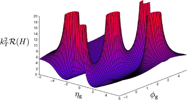
Figure 2: Antenna pattern for $qq^{\prime}\rightarrow qq^{\prime}H\,;\,H\rightarrow b\bar{b}$. Here $\eta_{\textrm{jet}}=3.5$.

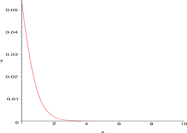
Figure 3: The point $(\eta_{\textrm{g}},\phi_{\textrm{g}})=(0,\pi/2)$ in ${\cal R}(qq^{\prime}\rightarrow qq^{\prime})$ as one varies $\eta_{\textrm{jet}}$. As the jets move apart, the antenna falls to zero.

One can clearly see that a colour connection exists between the initial state parton $p_{1}$ and final state jet $p_{3}$, similarly with $p_{2}$ and $p_{4}$, and also between the $b$-quark jets. The antenna pattern is small between the jets and the $b$’s as there is no colour connection between these — this is the ‘rapidity gap’ phenomenon. The emission of soft gluons in the rapidity gaps decreases as the gap widens. This is illustrated in the case without the $b$-quark antenna (Fig. 3), which shows the antenna pattern at $(\eta_{\textrm{g}},\phi_{\textrm{g}})=(0,\pi/2)$ as a function of $\eta_{\textrm{jet}}$.

Figure 4: Electroweak $Z$ production.

Next we consider the analogous electroweak $Z$ production process (Fig. 4), which can in principle be used to calibrate the Higgs production process. In this case the variety of diagrams at leading order means that there is no exact eikonal factorisation. However in the kinematic limit we are interested in — forward jets and central $Z$ production — the dominant amplitude is again the one involving $t$–channel $W$ exchange, i.e. $WW\to Z$, and the antenna pattern is trivially identical to that for Higgs production. We will prove this result, and consider its implications, when we discuss how to calculate antenna patterns numerically below.

2.2 QCD $Z$ Production

Figure 5: QCD $Z+2$ forward jet production.

In practice, $Z+2\;$jet production can also occur by ${\cal O}(\alpha_{S}^{2}\alpha_{W})$ QCD production involving $t$-channel gluon exchange, see Fig. 5d. Because of the different colour structure of such diagrams we would expect a very different antenna pattern.

Once again there is no exact factorisation of an overall soft gluon form factor and therefore no simple expression for the radiation pattern. However, as for electroweak $Z$ production the factorisation is restored in the forward jet – central $Z$ limit, in which case the antenna pattern is identical to that for the QCD ${\cal O}(\alpha_{S}^{2})$ $qq^{\prime}\to qq^{\prime}$ production process [9], i.e.

$$\mathcal{R}(QCD\,\,Z)\to 2C_{F}([14]+[23])+\frac{1}{N_{c}}[12;34]+2C_{F}[56],$$ (2.9)

where

$$[ij;kl]\equiv 2[ij]+2[kl]-[ik]-[il]-[jk]-[jl].$$ (2.10)

Substituting the kinematics of Eq. (2.1) and plotting the resulting analytic expression with $\eta_{\textrm{jet}}=3.5$, one obtains Figure 6.

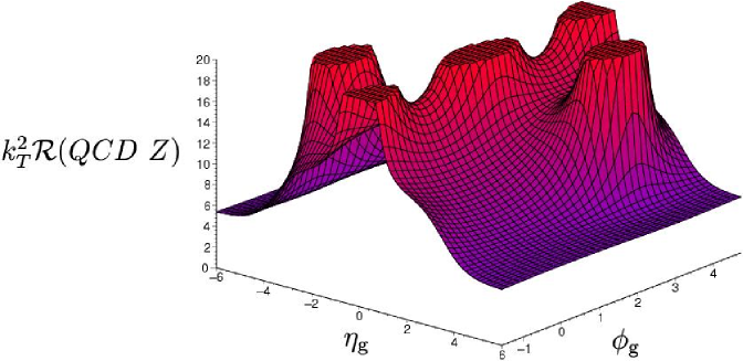
Figure 6: Antenna pattern for $qq^{\prime}\rightarrow qq^{\prime}Z\,\textrm{(QCD)}\,;\,Z\rightarrow b\bar{b}$ with $\eta_{\textrm{jet}}=3.5$.

Before commenting on the differences, we note that both Figures 2 and 6 exhibit the same limiting behaviour

$$\lim_{|\eta_{g}|\rightarrow\infty}k_{T}^{2}\mathcal{R}(H,QCD\,\,Z)=4C_{F},$$ (2.11)

as a consequence of both processes having initial state quarks. They are also identical as one approaches the collinear singularities corresponding to the final state $b$–jets:

$$\lim_{(\eta_{\textrm{g}},\phi_{\textrm{g}})\rightarrow(\eta_{\textrm{jet}},\phi_{\textrm{jet}})}k_{T}^{2}\mathcal{R}(H,QCD\,\,Z)\rightarrow 4C_{F}\frac{1}{\cosh^{2}(\eta_{\textrm{g}}-\eta_{\textrm{jet}})-\cos^{2}(\phi_{\textrm{g}}-\phi_{\textrm{jet}})}.$$ (2.12)

The difference in the colour flow shows up in the region between the two final state forward quark jets, as expected. Taking the ratio of the two patterns makes this difference plain (Fig. 7). The maximum difference occurs at $(\eta_{\textrm{g}},\phi_{\textrm{g}})=(-4.4,0)$ and $(\eta_{\textrm{g}},\phi_{\textrm{g}})=(4.4,\pi)$ when the ratio attains the value $2.3$. This shows the colour connection between the initial state (at $\eta_{\textrm{g}}=\pm\infty$) and the forward jets in the Higgs production case that is suppressed by a factor ${\cal O}(\frac{1}{N_{c}^{2}})$ in the QCD Z-production case. Another interesting phase space point is at $(\eta_{\textrm{g}},\phi_{\textrm{g}})=(0,0)$, i.e. the central region transverse to the $b\bar{b}$ axis. Here the radiation pattern increases by a factor of three going from Higgs to QCD $Z$ production, indicating the presence of an additional underlying colour connection in the latter case.

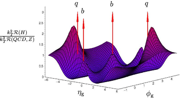
Figure 7: Ratio of Higgs to QCD $Z$ production antenna patterns. The ratio is unity at the position of the jets (indicated by arrows) and in the forward and backward limits $|\eta_{\textrm{g}}|\rightarrow\infty$.

3 Numerical Hadronic Antenna Patterns

An important (and dominant) background to the processes considered in the previous section comes from QCD ${\cal O}(\alpha_{S}^{3})$ $b\bar{b}+2\;$ jet production when $M_{b\bar{b}}\sim M_{H,Z}$. Some sample diagrams are shown in Fig. 8. There is clearly no unique and simple colour flow associated with these diagrams, and hence no compact analytic antenna pattern can be derived. This is an example of a situation where there is no factorisation of the form $(2\rightarrow 4\textrm{ matrix element})\times(\textrm{antenna factor})$.

Figure 8: Examples of QCD dijet plus $b\bar{b}$ production diagrams.

However we can instead use a purely numerical method in which we compare the values of the $2\rightarrow n$ and $2\rightarrow n+1$ matrix elements at each point in phase space, their ratio in the soft gluon limit defining the antenna pattern. In order to verify that this methodology works, and in particular to establish how soft the gluon has to be before the limiting pattern is reached to some level of precision, we first make a numerical evaluation of the analytic radiation patterns discussed in the previous section.

3.1 Comparison of Numerical and Analytic Antenna Patterns for Signal Processes

Unlike the analytic case, where we can simply ignore the momentum of the soft gluon in assigning a kinematic configuration that respects momentum conservation, we must account for the numerically finite gluon momentum in evaluating the matrix elements. Thus there is a degree of arbitrariness introduced. We choose to assign the momenta such that the central boson or $b\bar{b}$ system cancels the $3$-momentum of the soft gluon. In other words

$$p^{\mu}_{Z,H,b\bar{b}}=\left(\sqrt{m_{Z,H}^{2}+k^{2}},-\underline{k}\right).$$ (3.1)

Therefore the value of the antenna pattern depends on the specific $k_{T}$ that we choose for the soft gluon, but in such a way that $k_{T}^{2}\mathcal{R}$ tends to a finite limit as $k_{T}\to 0$. Figure 9 illustrates this by taking the ratio of the numerical $qq^{\prime}\rightarrow qq^{\prime}H$ antenna pattern with the analytic $qq^{\prime}\rightarrow qq^{\prime}$ antenna pattern for $k_{T\,g}=1$ GeV. The ratio is close to unity, except when the gluon rapidity is very large. In this region the ‘soft’ gluon carries a significant amount of energy and begins to distort the overall kinematics. For numerical purposes only, as a formal check that this effect is under control, we can set $k_{T\,g}$ to be sufficiently (and artificially) small to make sure the analytic result is recovered everywhere. Thus Fig. 10 shows the same ratio for $k_{T\,g}=10^{-5}$ GeV – no deviation from unity is now discernible. Note that we will always use $k_{T\,g}=1$ GeV in making predictions for the antenna patterns using the numerical treatment. Since our ultimate aim is to compare two numerically generated antenna patterns in signal to background studies, the discrepancies at large gluon rapidity visible in Fig. 9 will exactly cancel in the comparison.

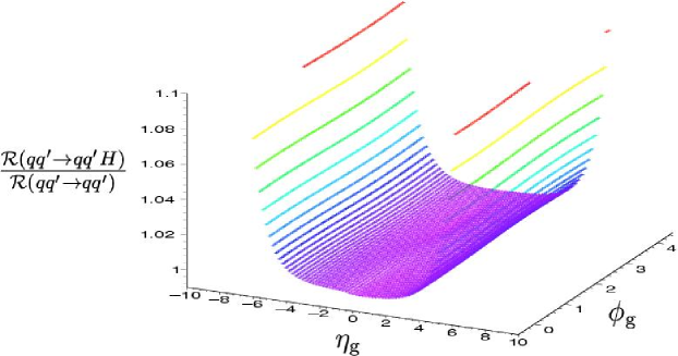
Figure 9: Ratio of numerical $qq^{\prime}\rightarrow qq^{\prime}H$ to analytic $qq^{\prime}\rightarrow qq^{\prime}$ antenna patterns with $|\eta_{\textrm{jet}}|=2$ and $k_{T\textrm{g}}=1$ GeV.

Figure 10: Ratio of numerical $qq^{\prime}\rightarrow qq^{\prime}H$ to analytic $qq^{\prime}\rightarrow qq^{\prime}$ antenna patterns with $|\eta_{\textrm{jet}}|=2$ and $k_{T\textrm{g}}=10^{-5}$ GeV.

As already pointed out, the antenna pattern for the full electroweak $qq^{\prime}\rightarrow qq^{\prime}Z$ process is not given by the simple analytic approximation, except when the jets are far forward. We can now illustrate this using the numerical method. Thus Figs. 11 and 12 show the ratio of the numerical electroweak $qq^{\prime}\rightarrow qq^{\prime}Z$ antenna pattern with the analytic electroweak $qq^{\prime}\rightarrow qq^{\prime}$ antenna pattern for the choice of $|\eta_{\textrm{jet}}|=2$ and $|\eta_{\textrm{jet}}|=4$ with $k_{T}=10^{-5}$ GeV. In the former case, the agreement with the analytic antenna pattern is only at the 10% level. The discrepancy is due to the contribution of the $Z$-sstrahlung diagrams (Fig. 4b) in the numerical case. However, as one forces the quark jets to be more forward the discrepancy decreases. Therefore, as long as we require the jets to be forward (i.e. $|t|\ll\sqrt{s}$), the analytic approximation is valid.

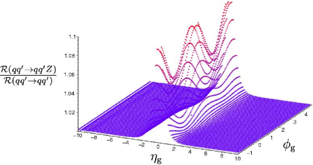
Figure 11: Ratio of numerical EW $qq^{\prime}\rightarrow qq^{\prime}Z$ to analytic $qq^{\prime}\rightarrow qq^{\prime}$ antenna patterns with $|\eta_{\textrm{jet}}|=2$ and $k_{T\textrm{g}}=10^{-5}$ GeV.

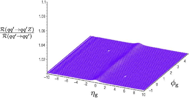
Figure 12: Ratio of numerical EW $qq^{\prime}\rightarrow qq^{\prime}Z$ to analytic $qq^{\prime}\rightarrow qq^{\prime}$ antenna patterns with $|\eta_{\textrm{jet}}|=4$ and $k_{T\textrm{g}}=10^{-5}$ GeV.

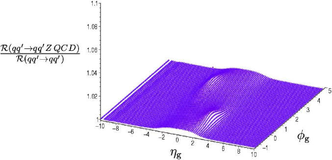
Figure 13: Ratio of numerical QCD $qq^{\prime}\rightarrow qq^{\prime}Z$ to analytic $qq^{\prime}\rightarrow qq^{\prime}$ antenna patterns with $|\eta_{\textrm{jet}}|=2$ and $k_{T\textrm{g}}=10^{-5}$ GeV.

Figures 13 and 14 show the same qualitative effect in the QCD mediated $Z$ production case. The deviation from our approximation that $|t|\ll\sqrt{s}$ is noticeably less than in the electroweak case. The reason for this is that in the electroweak case we are kinematically disturbing a delicate interplay between the numerator and the denominator in the term describing the colour connection between $p_{1}$ and $p_{3}$

$$[13]=\frac{p_{1}\cdot p_{3}}{(p_{1}\cdot k)(p_{3}\cdot k)}$$ (3.2)

In particular, due to the smallness of the numerator, this contribution is strongly suppressed for the radiation outside the narrow cones around the directions of the incoming and outgoing partons. Contrast this with the QCD $Z$ production case where the dominant colour connection is between $p_{1}$ and $p_{4}$

$$[14]=\frac{p_{1}\cdot p_{4}}{(p_{1}\cdot k)(p_{4}\cdot k)}$$ (3.3)

Here the numerator is not small. This cancellation is therefore more stable and our kinematic disturbance has less effect.

Figure 14: Ratio of numerical QCD $qq^{\prime}\rightarrow qq^{\prime}Z$ to analytic $qq^{\prime}\rightarrow qq^{\prime}$ antenna patterns with $|\eta_{\textrm{jet}}|=4$ and $k_{T\textrm{g}}=10^{-5}$ GeV.

3.2 Numerical Antenna Patterns for Background Processes

Figure 15 shows the numerical antenna pattern for the QCD mediated process $qq^{\prime}\rightarrow qq^{\prime}b\bar{b}$.

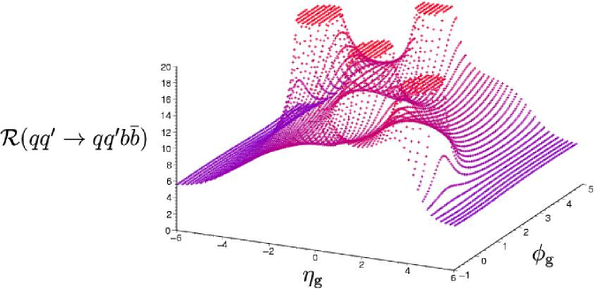
Figure 15: Numerical antenna pattern for $qq^{\prime}\rightarrow qq^{\prime}b\bar{b}$ with $|\eta_{\textrm{jet}}|=4$ and $k_{T\textrm{g}}=1$ GeV.

We will again focus mainly on the background process with initial state quarks, to allow comparison with the signal processes. In any case, the typical $\sqrt{\hat{s}}$ of the parton–level process is typically several TeV at the LHC, so we are working at high $x$ and quark initiated processes will dominate. Therefore the antenna patterns for the signal and background processes become identical near the beam and final state $b$–quark directions, being dominated by the (universal) collinear singularity for emission off quark lines.

Figure 16 shows the radiation pattern for the background QCD process $qg\rightarrow qgb\bar{b}$ with $|\eta_{\textrm{jet}}|=4$ and $k_{T\textrm{g}}=1$ GeV. As expected, the pattern is much more complicated than that for the signal $H$ or $Z$ production processes. Colour strings can now connect many more pairs of initial and final state particles, and the overall level of radiation is higher as a result. However in the directions of the incoming and outgoing partons, the distribution of soft radiation is the same as that for the signal processes. Thus, in particular, the distribution approaches $4C_{F}$ for large positive $\eta_{\textrm{g}}$, cf. Eq. (2.11).

For completeness, we show in Figs. 16 – 19 the corresponding antenna patterns for the other QCD $2\to 2+(b\bar{b})$ processes. The most obvious differences are in the size of the distributions near the incoming and outgoing partons, where the limiting $4C_{F}$ behaviour for emission off quarks is replaced by $4C_{A}$ for emission off gluons.

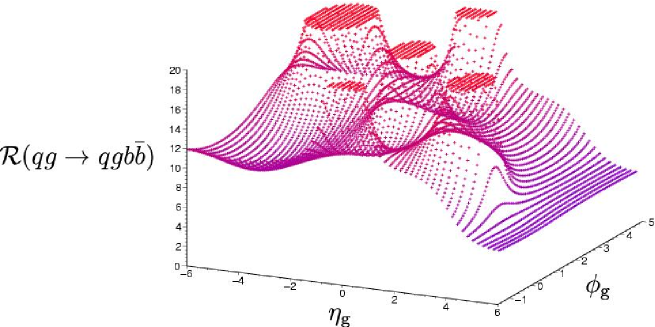
Figure 16: Numerical antenna pattern for $qg\rightarrow qgb\bar{b}$ with $|\eta_{\textrm{jet}}|=4$ and $k_{T\textrm{g}}=1$ GeV.

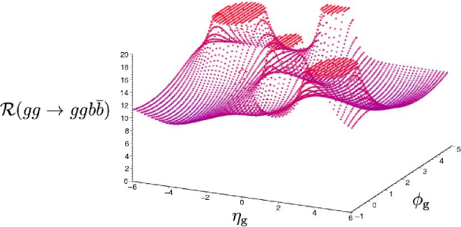
Figure 17: Numerical antenna pattern for $gg\rightarrow ggb\bar{b}$ with $|\eta_{\textrm{jet}}|=4$ and $k_{T\textrm{g}}=1$ GeV.

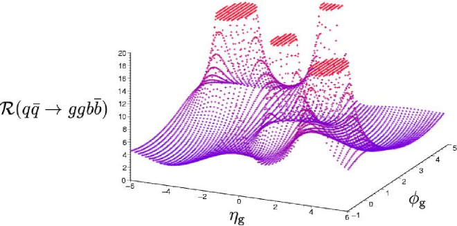
Figure 18: Numerical antenna pattern for $q\bar{q}\rightarrow ggb\bar{b}$ with $|\eta_{\textrm{jet}}|=4$ and $k_{T\textrm{g}}=1$ GeV.

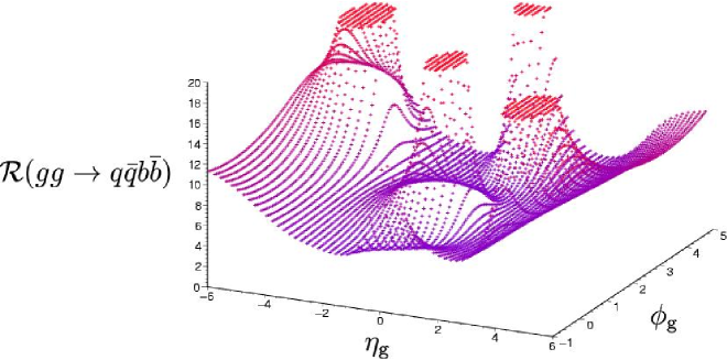
Figure 19: Numerical antenna pattern for $gg\rightarrow q\bar{q}b\bar{b}$ with $|\eta_{\textrm{jet}}|=4$ and $k_{T\textrm{g}}=1$ GeV.

The interesting quantities are of course the differences between the signals and backgrounds. Figure 20 shows the ratio of numerical $qq^{\prime}\rightarrow qq^{\prime}H;\,H\rightarrow b\bar{b}$ to numerical $qq^{\prime}\rightarrow qq^{\prime}b\bar{b}$ antenna patterns, for the same typical kinematic configuration as before, i.e. $|\eta_{\textrm{jet}}|=4$ and $k_{T\,g}=1$ GeV. We see that the ratio (i) falls to near zero between the central and forward particles (rapidity gap effect), (ii) is larger than one between the final-state $b\bar{b}$ pair, (iii) is larger than one between the forward jets and the beam (the [13] and [24] connection in the signal), and (iv) approaches unity in the forward/backward directions and at the locations (marked as arrows) of the incoming and outgoing particles. Over the whole $(\eta,\phi)$ plot, the ratio varies in size from a minimum of $0.03$ to a maximum of $2.3$, i.e. a factor of $70$. The corresponding ratio of the antenna patterns for the electroweak $Z$ production and QCD background is of course very similar.

We next consider (Fig. 21) the ratio of the QCD $Z$-production and background $qq^{\prime}\rightarrow qq^{\prime}b\bar{b}$ antenna patterns. There is much less structure here than there was in the corresponding Higgs case – note in particular that the rapidity gap dip between the forward and central particles is absent, and indeed that the ratio is close to one everywhere except near the central $b$ jets. In the $Z$ production case, there is always a colour string connecting the $b$ and the $\bar{b}$, and this results in the ratio increasing to a maximum of about 1.5 between these two particles. This value has a weak dependence on the rapidities of the forward jets. Figure  shows the slice through Fig. 21 at $\eta_{\textrm{g}}=0$ as $|\eta_{\textrm{jet}}|$ is varied from 1 to 8. The ratio is always one at $\phi_{\textrm{jet}}=\pi$ and $3\pi/2$, the location of the $b$ and $\bar{b}$.

Figure 20: Ratio of numerical $qq^{\prime}\rightarrow qq^{\prime}H;\,H\rightarrow b\bar{b}$ to numerical $qq^{\prime}\rightarrow qq^{\prime}b\bar{b}$ with $|\eta_{\textrm{jet}}|=4$ and $k_{T\,g}=1$ GeV.

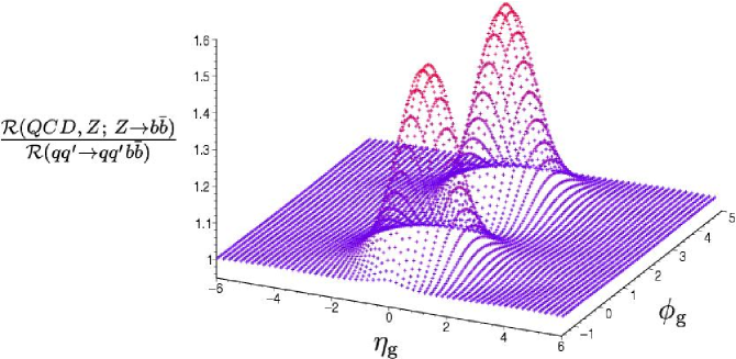
Figure 21: Ratio of numerical QCD $qq^{\prime}\rightarrow qq^{\prime}Z;\,Z\rightarrow b\bar{b}$ to numerical $qq^{\prime}\rightarrow qq^{\prime}b\bar{b}$ with $|\eta_{\textrm{jet}}|=4$ and $k_{T\,g}=1$ GeV.

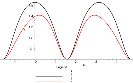
Figure 22: Slice in $\eta_{\textrm{g}}=0$ of Fig. 21 as the rapidity of the forward jets is varied.

4 Conclusions

Hadronic radiation patterns can provide a useful additional tool enabling us to improve the separation of Higgs production from the conventional QCD-induced backgrounds. In this paper we have focused on the vector boson fusion mechanism of Higgs production in the events with two forward tagging jets. We find that the fairly simple analytical expressions reflecting the coherent structure of QCD radiation off the multi-parton system (antenna pattern) can serve quite successfully as a qualitative guide for the more general numerical calculational technique, which in turn can be applied to a large variety of complicated processes.

The analysis presented here should be regarded as a ‘first look’ at the possibilities offered by hadronic flow patterns in searching for the Higgs in vector boson fusion. Of course, ultimately there is no substitute for a detailed Monte Carlo study including detector effects. However the results presented here indicate that the effects can be potentially large, and therefore that more detailed studies are definitely worthwhile.

References

-
[1]
Yu.L. Dokshitzer, V.A. Khoze and
S.I. Troyan, in Proc. 6th Int. Conf. on Physics in Collision,
ed. M. Derrick (World Scientific, Singapore, 1987), p.417.
Yu.L. Dokshitzer, V.A. Khoze and S.I. Troyan, Sov. J. Nucl. Phys. 46 (1987) 712. -
[2]
Yu.L. Dokshitzer, V.A. Khoze,
A.H. Mueller and S.I. Troyan, Rev. Mod. Phys. 60 (1988) 373.
V. A. Khoze and W. Ochs, Int. J. Mod. Phys. A12 (1997) 2949;
V. A. Khoze, W. Ochs and J. Wosiek, At the Frontier of Particle Physics, Ed. M. Shifman, v.2, 1101, [arXiv:hep-ph/0009298].
J. R. Andersen et al, J. Phys. G28 (2002) 2509 and references therein. - [3] Yu.L. Dokshitzer, V.A. Khoze, A.H. Mueller and S.I. Troyan, “Basics of Perturbative QCD”, ed. J. Tran Thanh Van, Editions Frontiéres, Gif-sur-Yvette, 1991.
-
[4]
R.K. Ellis, G. Marchesini and
B.R. Webber, Nucl. Phys. B286 (1987) 643; Erratum
Nucl. Phys. B294 (1987) 1180.
R.K. Ellis, presented at “Les Rencontres de Physique de la Vallee d’Aoste”, La Thuile, Italy, March 1987, preprint FERMILAB-Conf-87/108-T (1987). - [5] Yu.L. Dokshitzer, V.A. Khoze and S.I. Troyan, Sov. J. Nucl. Phys. 50 (1989) 505.
- [6] Yu.L. Dokshitzer, V.A. Khoze and T. Sjöstrand, Phys. Lett. B274 (1992) 116.
- [7] G. Marchesini and B.R. Webber, Nucl. Phys. B330 (1990) 261.
- [8] D. Zeppenfeld, Acta Phys. Polon. B27 (1996) 1653, [arXiv:hep-ph/9603315].
- [9] J. Ellis, V.A. Khoze and W.J. Stirling, Zeit. Phys. C75 (1997) 287.
- [10] V.A. Khoze and W.J. Stirling, Zeit. Phys. C76 (1997) 59.
- [11] J. Amundson, J. Pumplin and C. Schmidt, Phys. Rev. D57 (1998) 527.
-
[12]
V.A. Khoze, S. Lupia and W. Ochs,
Eur. Phys. J. C5 (1998) 77, [arXiv:hep-ph/9711392];
J. M. Butterworth, V. A. Khoze and W. Ochs, J. Phys. G25 (1999) 1457;
M. A. Buican, V. A. Khoze and W. Ochs, Eur. Phys. J. C28 (2003) 313.
C. F. Berger, T. Kúcs and G. Sterman, [arXiv:hep-ph/0212343].
C. F. Berger, T. Kúcs and G. Sterman, [arXiv:hep-ph/0303051]. - [13] M. Heyssler, V. A. Khoze and W. J. Stirling, Eur. Phys. J. C7 (1999) 475 [arXiv:hep-ph/9805490].
- [14] M.M. Heyssler and W.J. Stirling, Phys. Lett. B407 (1997) 259.
- [15] Ya.I. Azimov, Yu.L. Dokshitzer, V.A. Khoze and S.I. Troyan, Z. Phys. C27 (1985) 65; C31 (1986) 213.
- [16] CDF collaboration: F. Abe et al., Phys. Rev. D50 (1994) 5562.
- [17] D0 collaboration: B. Abbott et al., Phys. Lett. B414 (1997) 419; preprint FERMILAB-Conf-97-372-E; N. Varelas, preprint FERMILAB-Conf-97-346-E.
- [18] M. Carena and H. E. Haber, Prog. Part. Nucl. Phys. 50 (2003) 63 [arXiv:hep-ph/0208209].
- [19] ATLAS: Detector and physics performance technical design report, CERN-LHCC-99-14.
- [20] CMS Technical Proposal, CERN/LHC/94-43 LHCC/P1 (December 1994).
- [21] V. A. Khoze, M. G. Ryskin, W. J. Stirling and P. H. Williams, Eur. Phys. J. C26 (2003) 429 [arXiv:hep-ph/0207365].
- [22] A. B. Kaidalov, V. A. Khoze, A. D. Martin and M. G. Ryskin, Eur. Phys. J. C21 (2001) 521.
- [23] V. A. Khoze, A. D. Martin and M. G. Ryskin, Eur. Phys. J. C23 (2002) 311.
- [24] Ya.I. Azimov, Yu.L. Dokshitzer, V.A. Khoze and S.I. Troyan, Phys. Lett. B165 (1985) 147.
- [25] V.A. Khoze, J. Ohnemus and W.J. Stirling, Phys. Rev. D49 (1994) 1237.
- [26] Yu.L. Dokshitzer, V.A. Khoze and S.I. Troyan, J. Phys. G17 (1991) 1481; ibid. G17 (1991) 1602; Phys. Rev. D53 (1996) 89.
- [27] A. De Roeck, V. A. Khoze, A. D. Martin, R. Orava and M. G. Ryskin, Eur. Phys. J. C 25 (2002) 391 [arXiv:hep-ph/0207042].
- [28] H. Chehime and D. Zeppenfeld, Phys. Rev. D 47 (1993) 3898.