Lifetime of Kaonium

Abstract

The kaon–antikaon system is studied in both the atomic and the strongly interacting sector. We discuss the influence of the structures of the $f_{0}(980)$ and the $a_{0}(980)$ mesons on the lifetime of kaonium. The strong interactions are generated by vector meson exchange within the framework of the standard $SU(3)_{V}\times SU(3)_{A}$ invariant effective Lagrangian. In the atomic sector, the energy levels and decay widths of kaonium are determined by an eigenvalue equation of the Kudryavtsev–Popov type, with the strong interaction effects entering through the complex scattering length for $K\bar{K}$ scattering and annihilation. The presence of two scalar mesons, $f_{0}(980)$ and $a_{0}(980)$, leads to a ground state energy for the kaonium atom that is shifted above the point Coulomb value by a few hundred eV. The effect on the lifetime for the kaonium decay into two pions is much more dramatic. This lifetime is reduced by two orders of magnitude from $1.2\times 10^{-16}$ sec for annihilation in a pure Coulomb field down to $3.2\times 10^{-18}$ sec when the strong interactions are included. The analysis of the two photon decay width of the $f_{0}(980)$ suggests a generalization of the molecular picture which reduces the lifetime of kaonium still further to $1.1\times 10^{-18}\textrm{ sec}$.

I Introduction

There has been substantial experimental progress in the field of meson spectroscopy during the last decade amsler . In the energy region up to 2 GeV, more scalar-isoscalar mesons have been established than can be accounted for by a quark-antiquark structure godfrey . The structure of the scalar meson with lowest mass, the $f_{0}(980)$, has been controversial for many years. The $f_{0}(980)$ might be a $q\bar{q}$ state Montanet2000 ; Anisovich2000 , a $q^{2}\bar{q}^{2}$ state achasov82 , or a $K\bar{K}$ molecule WS90 .

The radiative decay of the $\phi$-meson provides a particularly strong argument for a $q^{2}\bar{q}^{2}$ interpretation of both the $f_{0}(980)$ and the $a_{0}(980)$ mesons, as was first pointed out by N.N. Achasov and V.N. Ivanchenkoachasov82 . Both the recent Novosibirsk dataachassov00 and the KLOE dataKLOE can be reproduced by a calculation which generates those mesons dynamically, howeveroller03 . Since in Ref.oller03 Oller had to introduce a $\phi\rightarrow\gamma K^{0}\bar{K}^{0}$ contact interaction, the issue remains controversialachasov03 .

The production of two neutral pions in ultrarelativistic pion proton reactions shows a strong dependence of the S-wave amplitude on the momentum transferred between the proton and the neutron for invariant two-pion masses in the vicinity of 1 GeVgams ; gunter01 . This fact has been interpreted as evidence for a hard component of the $f_{0}(980)$, see e.g. Ref. Achasov1 . A recent calculation based on a model which allows for a dynamical generation of the $f_{0}(980)$ provides a good description of the datasassen03 . On the other hand, the model employed in Ref.sassen03 also includes a bare scalar resonance. Given this situation, we feel that a simplified calculation might be helpful.

In this paper, we develop an analytical model which generates the $f_{0}(980)$ meson as a bound $K\bar{K}$ structure. This model makes specific predictions for the structure of the exotic atom Kaonium. In a second step, we work out the predictions for Kaonium based on the meson-exchange model of Ref.sassen03 .

The molecular interpretation is consistent with the small binding energy $\sim 10$–$20$ MeV of the $K\bar{K}$ system relative to its reduced mass $M_{K}\approx 496$ MeV. This suggests a non–relativisic effective field theory approachLLR02 that has also been used recently to study both pioniumGLRG01 ; HadAtom02 as well as ${\cal O}(\alpha^{6})$ QED recoil and radiative corrections to the positronium spectrumCMY99 . With this in mind we use the standard $SU(3)_{V}\times SU(3)_{A}$ LagrangiandeSwart63 to describe the dynamics of the $K\bar{K}$ interactionLohse90 ; Jansen95 and decay via the exchange of $\rho,\omega,\phi,K^{*}....$ vector mesons. The coupling constants appearing in the Lagrangian are related via $SU(3)$ symmetry to the $\rho\pi\pi$ coupling constant $g_{\rho\pi\pi}$, which in turn can be obtained from the KSRF relationKSRF66 . Thus once the decision on the form of Lagrangian has been taken, only physical meson masses and known coupling constants enter into the calculations.

We work in the non–relativistic limit in which case two important simplifications occur: (i) only $t$–channel exchange diagrams survive, and (ii) the resulting one–meson exchange potentials become local. This in turn means that one can reduce the Bethe–Salpeter (BS) integral equation for the bound states of the interacting $K\bar{K}$ system to a local two–body Schroedinger wave equation that offers a significant simplification over working with integral equationsLohse90 ; Sassen01 .

After a brief recall of the derivation of the wave equation for non–relativistic local potentials from the BS equation in Section II, the calculation of one meson exchange potentials involving both direct $\rho,\omega,\phi$ transfer between $K$ and $\bar{K}$ as well as $K\bar{K}\to K\bar{K}$ scattering via two–pion intermediate states involving $K^{*}$ exchanges is carried out in Section III. We refer to these potentials collectively as one–boson exchange (OBE) potentials. The last contribution is essential to describe the $K\bar{K}\to 2\pi$ decay channel. Then we make use of the fact that one can describe the low–energy properties of $K\bar{K}$ very adequately in the effective range approximation, to replace the OBE potentials by phase–equivalent potentials of the Bargmann typeBargmann49 that give rise to the same scattering length and effective range. These potentials offer the unique advantage of having known analytic solutions so that the associated Jost functions can be constructed explicitly.

A knowledge of the Jost functions in turn determines both the scattering and bound state properties of the $K\bar{K}$ system without futher approximationNewton56 . In Section IV we carry out this program and compute both the mass and decay width of the kaonic molecule from the relevant Jost function that includes annihilation contributions. The resulting complex total energy for this system is $(981-25i)$ MeV that is in reasonable agreement with the recent experimental data from Fermilabfermilab2001 that give $[(975\pm 3)-(22\pm 2)i]$ MeV.

We also give computed elastic and reaction cross sections for $K\bar{K}$ scattering, the $\pi\pi$ inelasticities, and the cross section for the inverse process, $\pi^{+}\pi^{-}\to K\bar{K}$, for which data exists, using detailed balance. Those calculations disagree with the measured cross section, particularly near thresholdSDP73 ; ADM77 ; BHyams1973 .

On the other hand the similarity in the pole position in both the recent Fermilab measurements as well as the calculated position of this pole is striking. We also show that the molecular picture is totally inadequate for describing the 2 photon decay width of $f_{0}(980)$, which comes out to be an order of magnitude larger than experiment. Taken together with the overall underestimate of the $\pi^{+}\pi^{-}\to K\bar{K}$ data, this suggests that the $f_{0}(980)$ ground state cannot be a pure molecular state (see alsoDeser54 ). This point is taken further at the end of Section IV.

We take up the discussion of kaonium in Section V. Since kaonium is a mixture of isoscalar and isovector states due to isospin–breaking introduced by the Coulomb potential, we appeal to the no–internal–mixing approximation that was introduced in connection with isobaric analog states in nuclei. In this approximation one joins linear combinations of the $I=0$ and $I=1$ isospin amplitudes in the external region where only the Coulomb field is important, onto (in this case) known solutions of good isospin of the wave equation in the internal region where the strong field is dominant. This allows one to construct the Jost function for kaonium without further approximation. Only momenta of ${\cal O}(M_{K}\alpha)$, where $\alpha\approx 1/137$, are of interest for kaonium. This fact allows one to recast the condition that its bound states are given by the zeros of the Jost function in the lower half of the complex momentum plane as an eigenvalue equation of the Kudryavtsev–Popov typeKP79 , in which the strong field effects only enter through the $K^{+}K^{-}$ scattering length. The solutions of this equation show that the kaonium levels are shifted upwards from their pure Coulomb values and acquire lifetimes between $10^{-18}$–$10^{-16}$ sec in the presence of the $K\bar{K}$ molecular ground state.

We also show explicitly that the strong field introduces an additional node into the eigenfunctions of kaonium that lies at the $K^{+}K^{-}$ scattering length. The kaonium levels are therefore to be viewed as excited states of the kaonic molecule in the combined Coulomb and strong fields of the system. This in turn has the effect of enhancing the $K^{+}K^{-}\to 2\pi$ annihilation widths by two orders of magnitude over what they would have been under Coulomb binding of the charged kaon pair alone.

II formalism

In order to obtain a non–relativistic equation for describing possible bound states of a $K\bar{K}$ meson pair resulting from vector meson exchange between them we briefly recall the derivation given by Landau and LifshitzLL82 that starts out with the four–point vertex $i\Gamma[p_{3},p_{4};p_{1},p_{2}]$ that enters the Bethe–Salpeter (BS) equation. The $p_{1},p_{2}$ and $p_{3},p_{4}$ are incoming and outgoing meson four momenta respectively. Then the homogeneous equation for this vertex that determines the bound state poles of the BS equation is

$$i\Gamma[p_{3},p_{4};p_{1},p_{2}] = \int\frac{d^{4}q}{(2\pi)^{4}}i\hat{\Gamma}[p_{3},p_{4};q,p_{3}+p_{4}-q](-i)D(q)(-i)D(p_{3}+p_{4}-q)i\Gamma[q,p_{3}+p_{4}-q;p_{1}p_{2}]$$ (1)

All momentum labels formally flow from right to left, and the sum of each pair on either side of the semi–colon equals the total four momentum $P$ of the incoming pair which is conserved throughout the diagrammatic equation. The hatted vertex is the irreducible piece that generates $\Gamma$ by iteration. The $D^{\prime}s$ are meson propagators. For a free meson of four momentum $q$ and mass $M$ one has

$$-iD(q)=\frac{i}{q^{2}-M^{2}+i0}\approx(\frac{1}{2M})\frac{i}{q_{0}-M-{\bf q}^{2}/2M+i0}$$ (2)

if in addition we move to the non–relativistic limit by formally suppressing propagation “backwards” in time, i.e. by omitting the anti–particle pole in the upper half of the complex $q_{0}$ plane. We noteLL82 that the momenta $p_{1},p_{2}$ are simply labels in (1) that are not determined by the equation at all. So one can simply drop them. The other simplification is to observe that the combination

$$\chi(p_{3},p_{4})=D(p_{3})\Gamma[p_{3},p_{4}]D(p_{4})$$ (3)

appears under the integral sign. Thus one can equally well recast Eq. (1) as an integral equation for $\chi(p_{3},p_{4})$. This is most usefully written down in the center of mass (CM) system for which $[p_{3},p_{4}]=\pm p+P/2$ with $p=[p_{0},\bf p]$ and $P=[P_{0},0]$, where $P_{0}$ is the total energy in the CM frame. Then the equation determining the bound states readsLL82

$$i\chi(p,P)=D(p+\frac{1}{2}P)D(-p+\frac{1}{2}P)\int\frac{d^{4}q}{(2\pi)^{4}}\hat{\Gamma}[p+\frac{1}{2}P,-p+\frac{1}{2}P;q+\frac{1}{2}P,-q+\frac{1}{2}P]\chi(q,P)$$

(4)

where $\chi(p_{3},p_{4})=\chi(p+P/2,-p+P/2)\equiv\chi(p,P)$.

To make further progress towards a non–relativistic equation, the vertex $\hat{\Gamma}$ should not depend on the time components of the relative outgoing and incoming four momenta $p=[p_{0},\bf p]$ and $q=[q_{0},\bf q]$, i.e.

$$\hat{\Gamma}[p+\frac{1}{2}P,-p+\frac{1}{2}P;q+\frac{1}{2}P,-q+\frac{1}{2}P]\approx\hat{\Gamma}[{\bf p},{\bf q},P_{0}]$$ (5)

Should this be the case one can then integrate out these time components from $\chi$ to obtain what is effectively the $3D$ fourier transform of the wave function for relative motion,

$$\psi({\bf p})=\int_{-\infty}^{\infty}\frac{dp_{0}}{2\pi}\chi(p,P)$$ (6)

Carrying out the integrals over the time components of the relative four momenta one finally arrives at the desired equation,

$$(\frac{{\bf p^{2}}}{M}+2M-P_{0})\psi({\bf p})-\int\frac{d^{3}{\bf q}}{(2\pi)^{3}}\frac{\hat{\Gamma}[{\bf p},{\bf q},P_{0}]}{4M^{2}}\psi({\bf q})=0$$ (7)

that makes use of the non–relativistic approximation

$$\int_{-\infty}^{\infty}\frac{dp_{0}}{2\pi i}D(p+\frac{1}{2}P_{0})(D(-p+\frac{1}{2}P_{0})\approx\frac{1}{4M^{2}}\Big{(}\frac{1}{{\bf p^{2}}/M+2M-P_{0}}\Big{)}$$ (8)

as given by Eq. (2). One recognises Eq. (7) as the Schroedinger wave equation in momentum space for relative motion in a potential

$$V({\bf p},{\bf q})=-\frac{\hat{\Gamma}[{\bf p},{\bf q},P_{0}]}{4M^{2}}$$ (9)

and binding energy $\varepsilon=2M-P_{0}\geq 0$. Should $\hat{\Gamma}[{\bf p},{\bf q},P_{0}]$ only depend on the difference $\bf{p-q}$, the corresponding potential will be local in coordinate space. Since $\hat{\Gamma}$ is a $relativistic$ proper vertex that in lowest order gives the $T$ matrix, the mass factor $1/4M^{2}$ that converts $\hat{\Gamma}$ into a non–relativistic potential is the same factorGLRG01 that relates the relativistic $T$ matrix to its non–relativistic counterpart.

III One boson exchange potentials

In the following we use Eq. (9) to investigate the possible binding of the $K\bar{K}$ system via one-boson exchange potentials by constructing $\hat{\Gamma}$ from the relevant pieces of the standard $SU(3)_{V}\times SU(3)_{A}$ invariant Lagrangian, the derivation and properties of which are described in detail in Ref. deSwart63 . For $K\bar{K}$ scattering the relevant interaction Lagrangians for our purposes are

$${\cal L}_{KK\rho}=g_{KK\rho}[K^{\dagger}\vec{\tau}\partial_{\mu}K]\vec{\rho}^{\mu}+cc$$

$${\cal L}_{KK\omega}=g_{KK\omega}[K^{\dagger}\partial_{\mu}K]\omega^{\mu}+cc$$

$${\cal L}_{KK\phi}=g_{KK\phi}[K^{\dagger}\partial_{\mu}K]\phi^{\mu}+cc$$ (10)

which, together with

$${\cal L}_{\pi KK^{*}}=g_{\pi KK^{*}}[\partial^{\mu}\vec{\pi}\cdot K^{\dagger}\vec{\tau}K^{*}_{\mu}-\vec{\pi}\cdot\partial^{\mu}K^{\dagger}\vec{\tau}K^{*}_{\mu}]+cc$$ (11)

generate interaction potentials for $K\bar{K}\to K\bar{K}$ scattering via $\rho,\omega,\phi$ vector meson exchange, as well as for $K\bar{K}\to\pi\pi$ annihilation via $K^{*}(892)$ strange meson exchange. The $K^{\prime}s$ are all isospin doublets and $cc$ stands for the additional charge conjugation contribution with $K\to\bar{K}$, $K^{*}\to\bar{K}^{*}$.

The coupling constants in these expressions are all fixed in terms of the $\rho\pi\pi$ coupling constant $g_{\rho\pi\pi}$ by $SU(3)$ symmetry relationsdeSwart63 ,

$$g_{KK\rho}=g_{\bar{K}\bar{K}\rho}=\frac{1}{2}g_{\rho\pi\pi}$$

$$g_{KK\omega}=g_{\bar{K}\bar{K}\omega}=-\frac{1}{2}g_{\rho\pi\pi}$$

$$g_{KK\phi}=g_{\bar{K}\bar{K}\phi}=\frac{1}{\sqrt{2}}g_{\rho\pi\pi}$$

$$g_{\pi KK^{*}}=g_{\pi\bar{K}\bar{K}^{*}}=-\frac{1}{2}g_{\rho\pi\pi}$$ (12)

On the other hand the $\rho\pi\pi$ coupling is determined by the KSRF relationKSRF66 as $g_{\rho\pi\pi}\approx M_{\rho}/(\sqrt{2}f_{\pi})\approx 6$ in terms of the $\rho$ meson mass $M_{\rho}$ and the pion weak decay constant $f_{\pi}\approx 93$MeV. In this sense, then, there are no free parameters in the calculation of the exchange potentials. They only contain physical meson masses and known coupling constants.

In the non–relativistic limit, $p_{i}+p_{j}\approx[M_{i}+M_{j},0]$, $p_{i}-p_{j}\approx[0,{\bf p}_{i}-{\bf p}_{j}]$ only the $t$–channel scattering diagrams are relevant for determining $\hat{\Gamma}$. In this limit these amplitudes all have a common Yukawa–like form

$$\hat{\Gamma}[p+\frac{1}{2}P,-p+\frac{1}{2}P;q+\frac{1}{2}P,-q+\frac{1}{2}P]\approx g^{2}C_{I}n_{s}\frac{(M_{1}+M_{3})(M_{2}+M_{4})}{M^{2}+{\bf k}^{2}}$$ (13)

in momentum space, where ${\bf k}={\bf p}-{\bf q}$ is the $t$ channel $3$–momentum transfer, and $M_{i}$ are the masses in the indicated entrance and exit channels; M is the mass of the exchanged boson and $g$ the coupling constant. The isospin and boson identity factors $C_{I}$ and $n_{s}$ in Eq. (13) are given inLohse90 . They are $C_{0}=[3,1,1]$ and $C_{1}=[-1,1,1]$ and $n_{s}=1$ for $\rho,\omega,\phi$ exchange in the $K\bar{K}\to K\bar{K}$ isoscalar and isovector channels. The corresponding values for $K^{*}$ exchange in the $K\bar{K}\to\pi\pi$ isoscalar and isovector channels are $C_{0}=-\sqrt{6}$, $C_{1}=-2$, and $n_{s}=1/\sqrt{2}$.

III.1 $K\bar{K}$ exchange potentials

Since $\hat{\Gamma}$ is only a function of the $3$–momentum transfer, the resulting potentials in Eq. (9) are attractive local Yukawa potentials in coordinate space, and the determination of their possible bound states is numerically straightforward. While not necessary for convergence in the non–relativistic case, we, however, also include at each vertex in Eq. (13) the form factor containing an arbitrary cutoff $\Lambda$

$$F^{t}({\bf k})=\Big{(}\frac{2\Lambda^{2}-M^{2}}{2\Lambda^{2}+{\bf k}^{2}}\Big{)}^{2}$$ (14)

that was used in Lohse90 ; Sassen01 to obtain convergence in scattering calculations based on the relativistic $\hat{\Gamma}$ vertices. ¿From Eq. (9) the coordinate space non–relativistic $K\bar{K}\to K\bar{K}$ potential associated with the exchange of boson $M$ is then

$$V(r)=-g^{2}C_{I}U(M,r)$$ (15)

after division by $4M_{K}^{2}$ where $M_{K}$ is the kaon mass, and $U(M,r)$ is the fourier transform

$$U(M,r)=\int\frac{d^{3}{\bf k}}{(2\pi)^{3}}\frac{[F^{t}({\bf k})]^{2}}{M^{2}+{\bf k}^{2}}e^{i\vec{k}\cdot\vec{r}}=$$

$$\frac{1}{4\pi}\Big{\{}\frac{e^{-Mr}}{r}-\frac{e^{-\sqrt{2}\Lambda r}}{r}\Big{[}1+\frac{1}{16}(11-\frac{M^{2}}{2\Lambda^{2}}+\frac{M^{4}}{4\Lambda^{4}})(1-\frac{M^{2}}{2\Lambda^{2}})(\sqrt{2}\Lambda r)+$$

$$\frac{1}{16}(3-\frac{M^{2}}{2\Lambda^{2}})(1-\frac{M^{2}}{2\Lambda^{2}})^{2}(\sqrt{2}\Lambda r)^{2}+\frac{1}{48}(1-\frac{M^{2}}{2\Lambda^{2}})^{3}(\sqrt{2}\Lambda r)^{3}\Big{]}\Big{\}}$$ (16)

The resulting $K\bar{K}$ potential due to $\rho,\omega,\phi$ exchange are attractive in both isospin channels $I=0$ and $1$,

$$V_{I=0}(r)=-g^{2}_{\rho\pi\pi}\Big{\{}\frac{3}{4}U(M_{\rho},r)+\frac{1}{4}U(M_{\omega},r)+\frac{1}{2}U(M_{\phi},r)\Big{\}}$$ (17)

and

$$V_{I=1}(r)=-g^{2}_{\rho\pi\pi}\Big{\{}-\frac{1}{4}U(M_{\rho},r)+\frac{1}{4}U(M_{\omega},r)+\frac{1}{2}U(M_{\phi},r)\Big{\}}$$ (18)

but too weakly so in the latter channel due to an almost complete cancellation between $\rho$ and $\omega$ exchange to support a bound state. In deriving these expressions we have exploited the $SU(3)$ relations (12) to express all coupling constants in terms of $g_{\rho\pi\pi}$.

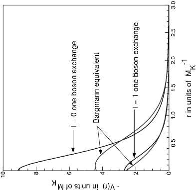
Figure 1: One boson exchange potentials using a cutoff of $\Lambda$ = 4 GeV. The coupling constant is $\alpha_{s}=2.9$ and the masses of the exchanged mesons are ($M_{\rho},M_{\omega},M_{\phi})=(769,783,1019)$ MeV. The analytical Bargmann potentials that reproduce the same scattering lengths and effective ranges as the original one boson exchange potentials are shown as companion curves.

These potentials are plotted in Fig. 1 for a strong coupling constant $\alpha_{s}=g^{2}_{\rho\pi\pi}/4\pi=2.9$ and cutoff $\Lambda=4$ GeV. In principle $\Lambda$ can be different for each exchanged bosonLohse90 . One notes that the $V_{I}$ are now finite at the origin, in contrast to the sum of pure Yukawa potentials to which they reduce as $\Lambda\to\infty$.

The coordinate space version of the wave equation Eq. (7) that describes the relative $s$–state motion in these potentials becomes the usual Schroedinger equation

$$[\bigtriangledown^{2}+k^{2}-M_{K}V_{I}(r)]\psi(r)=0$$ (19)

with total CM energy $P_{0}=2M_{K}+k^{2}/M_{K}$. We ignore the charged to neutral kaon mass difference and work with an average kaon mass $M_{K}$. By numerically constructing the $k\to 0$ scattering solutions one easily obtains the scattering lengths and effective ranges that enter into the effective range expansion of the $s$–wave phase shifts $\delta(k)$

$$k\cot\delta(k)=-\frac{1}{a_{I}}+\frac{1}{2}r_{I}k^{2}+\cdots$$ (20)

in the two channels as

$$a_{0}=5.835M^{-1}_{K},\quad r_{0}=1.187M^{-1}_{K}\quad({\rm isoscalar})$$

$$a_{1}=-0.401M^{-1}_{K},\quad r_{1}=3.702M^{-1}_{K}\quad({\rm isovector})$$ (21)

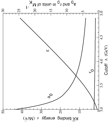
Figure 2: Dependence of the $K\bar{K}$ binding energy $\varepsilon$ (left hand scale), scattering length $a_{0}$ and effective range $r_{0}$ (right hand scale) on the choice of cutoff $\Lambda$ used in the form factor for the isosalar one boson exchange potential.

Thus only the isoscalar potential supports a bound state. Its binding energy is calculated to be $\varepsilon=18.63$ MeV, placing the total mass for the bound $K\bar{K}$ system at $P_{0}=2M_{K}-\varepsilon=973.4$ MeV. Fig. 2 illustrates the sensitivity of $\varepsilon$, $a_{0}$ and $r_{0}$ on the choice of cutoff for this channel. For $\Lambda\gtrsim 4$ GeV the values of $a_{0}$ and $r_{0}$ are only weakly dependent on $\Lambda$.

Even though the isovector potential does not support a bound state the $a_{0}(980)$ can be fully explained by this model as a threshold effect Jansen95 . Effects of the $a_{0}(980)$ thus are included in the calculation though it should be noticed that decays to the $\pi\eta$-channel are not considered in the analytical model.

III.2 Shape–independent approach

The relatively small (on a hadronic scale) binding energy $\varepsilon/M_{K}\sim 0.04$ in the isoscalar channel (and no binding at all in the isovector channel) indicates that an effective range approach should be applicable. This is confirmed by recalculating the binding energy from the effective range formulaNewton56 $\varepsilon\approx\kappa^{2}/M_{K}=18.60$ MeV where $\kappa=-a=0.194M_{K}$, see Eq. (27) below. Consequently it is entirely sufficient to characterize the $K\bar{K}$ interaction at low energies in terms of a scattering length and an effective range: the actual shape of the potential is immaterial.

We make use of this feature in the following to replace the strong potentials $V_{I}$ in Eqns.(17) and (18) by analytic potentials of the Bargmann type given below that are phase equivalent to them. BargmannBargmann49 (see alsoNewton60 for an in depth overview) has shown how to construct families of potentials that give rise to a prescribed Jost function $f(k)$. If one chooses

$$f(k)=\frac{k-ia}{k-ib}$$ (22)

then the potential that leads to this Jost function can be determined. It is Bargmann49 ; Newton60 ,

$$V_{I}(r)=-\frac{1}{M_{K}}\frac{8b^{2}}{b^{2}-a^{2}}\Big{[}\frac{e^{br}}{b-a}+\frac{e^{-br}}{b+a}\Big{]}^{-2}$$ (23)

For this potential the effective range expansion is exact:

$$k\cot\delta(k)=\frac{ba}{b-a}+\frac{k^{2}}{b-a}$$ (24)

This allows one to identify the scattering length and effective range as

$$a_{I}=-\frac{b-a}{ba},\quad r_{I}=\frac{2}{b-a}$$ (25)

where the actual values of the parameters $a$ and $b$ will depend on the isospin channel.

Fixing $a$ and $b$ is obviously equivalent to prescribing the scattering length and effective range. If $a$ is negative, $a=-\kappa$, say, then $f(k)$ has a zero at $k=-i\kappa$ in the lower half of the complex $k$ plane, and there is a bound stateNewton60 of binding energy $\varepsilon_{s}=\kappa^{2}/M_{K}$. Both the scattering and bound state wave functions of the Bargmann potential in Eq. (23) are known explicitly. Further details will be found in the Appendix. The availability of such analytic solutions will be important for including the effects of the $K\bar{K}\to\pi\pi$ decay channel non–perturbatively as discussed below.

Now invert Eq. (25) to construct phase equivalent potentials that have the same scattering length and effective range as the original exchange potentials in Eqs. (17) and (18). The required values of $a$ and $b$ are

$$a=- \frac{1}{r_{I}}\Big{[}1-\sqrt{1-2r_{I}/a_{I}}\Big{]}$$

$$b= \frac{1}{r_{I}}\Big{[}1+\sqrt{1-2r_{I}/a_{I}}\Big{]}$$ (26)

or

$$a=-0.1936{\rm M_{K}}\quad b=1.491{\rm M_{K}}\quad({\rm isoscalar})$$

$$a=+0.9219{\rm M_{K}}\quad b=1.462{\rm M_{K}}\quad({\rm isovector})$$ (27)

for the two channels in question. These parameters are summarized in Table 1 for easy reference. The resulting set of phase equivalent potentials are included in Fig. 1.

III.3 $K\bar{K}$ annihilation potential

¿From Eq. (13) one reads off the irreducible vertex for $K\bar{K}\to\pi\pi$ via $K^{*}$ exchange, as

$$\hat{\Gamma}(K\bar{K}\to\pi\pi)\approx-C_{I}n_{s}g^{2}_{\pi KK^{*}}\frac{(M_{\pi}+M_{K})^{2}}{M_{K^{*}}^{2}}$$ (28)

where $n_{s}C_{I}=-\sqrt{3}$ or $-\sqrt{2}$ in the isoscalar or isovector channel. We have neglected the $3$–momentum transfer relative to the large $K^{*}(892)$ mass. As shown in Fig. 3, this amounts to introducing point vertices that can contribute to $K\bar{K}$ scattering via an intermediate pion loop. The contribution from this interaction is complex due to the possibility of on–shell decays $K\bar{K}\to\pi\pi$ in the intermediate state, and the resulting $K\bar{K}$ bound state acquires a width. The details are as follows: calling the contribution from Fig. 3 $i\hat{\Gamma}^{(1)}$ one finds

$$i\hat{\Gamma}^{(1)} =i\hat{\Gamma}^{2}(K\bar{K}\to\pi\pi)\int\frac{d^{3}{\bf l}}{(2\pi)^{3}}\int_{-\infty}^{\infty}\frac{dl_{0}}{2\pi i}D(l+\frac{1}{2}P_{0})D(-l+\frac{1}{2}P_{0})$$ (29)

$$=i\hat{\Gamma}^{2}(K\bar{K}\to\pi\pi)\frac{1}{4M^{2}_{\pi}}\int\frac{d^{3}{\bf l}}{(2\pi)^{3}}\frac{1}{{\bf l}^{2}/M_{\pi}+2M_{\pi}-P_{0}}$$

$$=i\hat{\Gamma}^{2}(K\bar{K}\to\pi\pi)\frac{J(P_{0})}{4M^{2}_{\pi}}$$

in view of Eq. (8). As summarized briefly in Eqs. (107) and (108) of the Appendix the three dimensional integral $J(P_{0})$ can be dimensionally regulated in $d$ dimensions without difficulty to obtain a finite resultGLRG01 for $d\to 3$. The associated annihilation potential $V_{K\bar{K}}$ is then obtained from Eq. (9) as an attractive contact potential in coordinate space,

$$V_{K\bar{K}}(r)=-\frac{\hat{\Gamma}^{2}(K\bar{K}\to\pi\pi)}{(4M^{2}_{K})(4M^{2}_{\pi})}J(P_{0})\delta^{3}({\bf r})=-c^{2}_{0}\delta^{3}({\bf r})$$ (30)

with

$$c^{2}_{0}=\frac{3}{16}\frac{(g^{2}_{\pi KK^{*}})^{2}}{M_{\pi}^{2}M_{K}^{2}}\Big{(}\frac{M_{\pi}+M_{K}}{M_{K^{*}}}\Big{)}^{4}J(P_{0})\quad{(\rm isoscalar})$$ (31)

The value of this factor in the isovector channel is $c_{1}^{2}=\frac{2}{3}c_{0}^{2}$. The function

$$J(P_{0})=i\frac{M_{\pi}}{4\pi}\Big{[}M_{\pi}(P_{0}-2M_{\pi})\Big{]}^{1/2}$$ (32)

is a complex function of $P_{0}$ that is positive and pure imaginary along the upper lip of the branch cut extending from $2M_{\pi}$ to $\infty$ along the real $P_{0}$ axis, see Eq. (108).

III.4 Jost function for a finite plus delta function potential at the origin

We investigate the influence of the annihilation potential on the properties of the $K\bar{K}$ system by constructing the revised Jost function for the sum $V_{I}+V_{K\bar{K}}$. Since $V_{K\bar{K}}$ is a contact interaction, and the solutions in the potential $V_{I}$ are known, this can be done without approximation. The new scattering problem to be solved reads

$$[\bigtriangledown^{2}+k^{2}-M_{K}V_{I}(r)+M_{K}c^{2}_{I}\delta^{3}({\bf r})]\psi(r)=0$$ (33)

Consider isospin $I=0$. The presence of the delta function potential obliges one to give up the boundary condition $\varphi(k,r)\sim r\to 0$ on the scattering wave function $\varphi(k,r)=r\psi(k,r)$ at the origin in favor of prescribing its logarithmic derivative $\varphi^{\prime}/\varphi$ thereNewton60 . By integrating Eq. (33) over the volume of an infinitesimal sphere centered at the origin, one finds that the logarithmic derivative at the origin is fixed by the strength of the delta potential according to

$$\frac{\varphi^{\prime}}{\varphi}=\frac{4\pi}{M_{K}c^{2}_{0}}=\zeta$$ (34)

The point is now that for $r>0$ both the boundary condition on $\varphi(k,r)$ and the closed form of irregular solution of Eq. (33) are known explicitly: they are given by Eqs. (34) and (88) respectively. By constructing the Wronskian of this pair in the limit $r\to 0$ one obtains the revised Jost function as

$$f(k)=W[f,\varphi]=\Big{[}(\zeta+ik)\frac{k-ia}{k-ib}+i\frac{b^{2}-a^{2}}{k-ib}\Big{]}$$ (35)

after setting lim $\varphi(k,r)\to 1$ for convenience. This choice is unimportant since neither the root of $f(k)$ nor the scattering phase shift depends on it. The value of the logarithmic derivative $\zeta$ is $k$–dependent through $P_{0}$: from Eqs. (31) and (34) one finds

$$\zeta(k)=-\frac{256i}{3\alpha^{2}_{s}}M_{\pi}M_{K}\Big{(}\frac{M_{K^{*}}}{M_{K}+M_{\pi}}\Big{)}^{4}[M_{\pi}(P_{0}-2M_{\pi})]^{-1/2},$$

$$P_{0}=2M_{K}+\frac{k^{2}}{M_{K}}$$ (36)

after taking the $SU(3)$ value $g_{\pi KK^{*}}=-g_{\rho\pi\pi}/2$ for the coupling constant.

IV Numerical results

The single equation (35) contains all the necessary information on the scattering and bound states of the two–body $K\bar{K}$ system. Moreover, this information can be extracted without further approximation. We use this form of $f(k)$ to identify the revised scattering length and effective range as well as the bound state energy in the presence of $K\bar{K}\to 2\pi$ annihilation.

IV.0.1 Effective range expansion

The $K\bar{K}\to\pi\pi$ annihilation channel renders the scattering matrix $S(k)=f(k)/f(-k)$ non–unitary, since now $f^{*}(k)\neq f(-k)$. This can be seen directly from Eq. (35) after noting that the logarithmic derivative $\zeta$ is even in $k$ and purely negative imaginary for real $k$. The scattering phase shift is now complex. In order to identify the scattering length and effective range in the presence of absorption, one can either maintain the expansion (20), thereby introducing complex effective range parametersDeser54 ; KP79 , or definePetersen71 these in terms of the real part $\delta(k)$ of the total phase shift (not the phase of $S(k)$),

$$S(k)=f(k)/f(-k)=\eta e^{2i\delta(k)},\quad 0<\eta<1$$ (37)

In the latter case

$$k\cot\delta(k)=ik\frac{S(k)+\eta}{S(k)-\eta}=ik\frac{f(k)|f(-k)|+f(-k)|f(k)|}{f(k)|f(-k)|-f(-k)|f(k)|}$$ (38)

that shows explicitly that $k\cot\delta(k)$ is an even function of $k$. Set $\zeta(k)=-i\xi(k)$ in Eq. (35) for the Jost function, and then expand the right hand side to ${\cal O}(k^{2})$. After some calculation one establishes the revised effective range expansion

$$k\cot\delta(k)=-\frac{1}{a^{\prime}_{0}}+\frac{1}{2}r^{\prime}_{0}k^{2}+\cdots$$ (39)

with the exact expressions

$$-\frac{1}{a^{\prime}_{0}}=\frac{b}{b-a}\Big{\{}\frac{a^{2}\xi^{2}+(b^{2}-a^{2})^{2}}{a\xi^{2}-2ab^{2}+a^{3}-b^{3}}\Big{\}}$$ (40)

and

$$\frac{1}{2}r^{\prime}_{0}=\frac{a^{2}(b^{2}-a^{2})^{4}+a(b+a)[a^{3}(b-a)(5b^{2}-3a^{2})+b^{4}(a^{2}-2ab+2b^{2})]\xi^{2}}{(b-a)[a^{2}\xi^{2}+(b^{2}-a^{2})^{2}][a^{3}-b^{3}-2ab^{2}+a\xi^{2}]^{2}}+$$

$$\frac{a(b+a)[a(b-a)(b^{2}-3a^{2})-b^{4}]\xi^{4}+a^{4}\xi^{6}}{(b-a)[a^{2}\xi^{2}+(b^{2}-a^{2})^{2}][a^{3}-b^{3}-2ab^{2}+a\xi^{2}]^{2}}-$$

$$2\xi\xi^{\prime}ab^{4}\frac{[(a^{2}+ab-b^{2})(a^{3}-ab^{2}-b^{3})+a^{2}\xi^{2}(b+a)]}{(b-a)[a^{2}\xi^{2}+(b^{2}-a^{2})^{2}][a^{3}-b^{3}-2ab^{2}+a\xi^{2}]^{2}}$$ (41)

for the new inverse scattering length and effective range. Here

$$\xi=i\zeta=\frac{256}{3\alpha^{2}_{s}}M_{\pi}M_{K}\Big{(}\frac{M_{K^{*}}}{M_{K}+M_{\pi}}\Big{)}^{4}[M_{\pi}(2M_{K}-2M_{\pi})]^{-1/2}=17.409M_{K}$$

$$\xi^{\prime}=i\frac{\partial\zeta}{\partial k^{2}}=-\frac{128}{3\alpha^{2}_{s}}\sqrt{M_{\pi}}\Big{(}\frac{M_{K^{*}}}{M_{K}+M_{\pi}}\Big{)}^{4}[(2M_{K}-2M_{\pi})]^{-3/2}=-6.064M^{-1}_{K}$$ (42)

at $k=0$, and the primes serve to distinguish these scattering lengths and ranges from those appearing in Eq. (24), to which they reduce in the no annihilation limit $\xi\to\infty$. The numerical values of $\xi$ and $\xi^{\prime}$ have been calculated for meson masses $M_{\pi}=140$ MeV, $M_{K}=496$ MeV, $M_{K^{*}}=892$ MeV and coupling constant $\alpha_{s}=2.9$. Using these together with the values for $a$ and $b$ given in Table 1, one obtains

$$a^{\prime}_{0}=4.281M^{-1}_{K};\quad r^{\prime}_{0}=3.203M^{-1}_{K}\quad({\rm isoscalar})$$ (43)

as predictions for the $K\bar{K}$ isoscalar scattering length and effective range in the presence of absorption. The corresponding values for the isovector channel are still

$$a^{\prime}_{1}=-0.401M^{-1}_{K};\quad r^{\prime}_{1}=3.702M^{-1}_{K}\quad({\rm isovector})$$ (44)

since there is no annihilation contribution from the $l=0,\;I=1$ partial wave to the $K\bar{K}$ scattering amplitude due to the identity of the outgoing pions in the isospin representation. Higher partial waves cannot contribute in any event due to the contact nature of the annihilation interaction. In fact the $a_{0}(980)\to 2\pi$ decay channel is forbidden by $G$–parity. Thus the isovector scattering length remains real if, as here, the $\pi\eta$ decays are ignored.

IV.0.2 Bound states for $I=0$

The bound states of Eq. (33) are determinedNewton60 by the complex root(s) of $f(k)$ in Eq. (35), with Im$k<0$, i.e.

$$(\zeta(k)+ik)(k-ia)+i(b^{2}-a^{2})=0$$ (45)

Let $k=p-i\kappa$, $\kappa>0$ be such a root. Then the total mass $M$ and decay width $\Gamma$ of a bound $K\bar{K}$ pair at rest reads

$$P_{0}=M-\frac{i}{2}\Gamma=2M_{k}+\frac{(p-i\kappa)^{2}}{M_{K}}$$ (46)

This root can only be found numerically as will be done shortly. However, since the magnitude of the absorptive coupling $M^{2}_{K}|c^{2}_{0}|\sim 4\pi M_{K}/\xi\sim 0.7$ is quite small relative to the isoscalar potential strength, a perturbative solution in inverse powers of $\zeta$ is useful. Replace $\zeta$ by its value $-i\xi$ at $k=0$ (more correctly $k\approx-i\kappa$ but the difference is quantitatively insignificant). Then Eq. (45) reduces to a quadratic equation for $k$. The relevant root is

$$k=\frac{b^{2}-\kappa^{2}}{\xi}-i\kappa+O(\xi^{-2})\approx(0.1255-0.1936i)M_{K}$$ (47)

where $k=ia=-i\kappa=-0.1936M_{K}i$ is the root leading to the bound state in the absence of absorption, and $b=1.491M_{K}$. Working to the same order in $\xi^{-1}$ (i.e. neglecting the real part of $k$), one finds that

$$P_{0}\approx 2M_{K}-\frac{\kappa^{2}}{M_{K}}-2i\kappa\frac{(b^{2}-\kappa^{2})}{M_{K}\xi}$$ (48)

Since $4\pi\psi^{2}(0)=2\kappa(b^{2}-\kappa^{2})$ from Eq. (94) the result in Eq. (48) is equivalent to treating the annihilation potential $-c^{2}_{0}\delta^{3}({\bf r})$ as a first order perturbation of $P_{0}$,

$$P_{0}\approx 2M_{K}-\frac{\kappa^{2}}{M_{K}}-\frac{i}{2}\Gamma;\quad\Gamma=-2ic^{2}_{0}\psi^{2}(0)=\frac{8\pi}{M_{K}\xi}\psi^{2}(0)$$ (49)

Upon recalling that $-i\xi^{-1}\sim-J(P_{0})$, one sees from this form that the complex solution for $P_{0}$ always lies on the $second$ sheet $-2\pi\leq\phi\leq 0$ of the cut complex $P_{0}$ plane for $J(P_{0})$. Otherwise the signs of the imaginary parts of $P_{0}$ and $-J(P_{0})$ will differ, and no solution is possible. Taking cognizance of this fact the exact root of Eq. (45) and resulting value for $P_{0}$ are found numerically to be

$$k=(0.1254-0.1972i)M_{K};\quad P_{0}=(981-25i){\rm MeV}$$ (50)

using the the previously determined values of $a$ and $b$ shown in Table 1. Notice that the exact value of $k$ lies rather close to the perturbation estimate given by Eq. (47)

The exact numerical results for the Bargmann potential that is phase–equivalent to Eq. (17) are given in the first row of Table 2. We contrast these results with the mass and width calculations based on the Weinstein–Isgur non–relativistic potential modelWS90 , as well as the predictions of Morgan and PenningtonMP93 , based on a parametrization of the Jost function with parameters determined from experimental phase shifts. These calculations are also compared with the earlier experimental results summarized by the Particle Data Group (PDG)PDG92 , as well as the recent data from the Fermilab E791 Collaborationfermilab2001 .

In order to extract Bargmann potential parameters that would lead to the mass and width values of either Weinstein–Isgur, or Morgan and Pennington, we have turned Eq. (45) around and asked what values of $a$ and $b$ produce a root $k=p-i\kappa$ that gives a prescribed value of the complex total energy in Eq. (46). The answer is

$$a=-\kappa-p\frac{\nu+\kappa}{p-\xi}$$ (51)

$$b=\sqrt{a^{2}-p(p-\xi)+(\nu+\kappa)(a+\kappa)}$$ (52)

after setting $\zeta(p-i\kappa)=\nu-i\xi$. We have treated the experimental data in the same way. These relations allow one to establish a direct link between the mass and decay width of the bound $K\bar{K}$ state, and thence extract the isoscalar scattering length and effective range via Eqs. (40) and (41), or Eqs. (63) and (64).

The effective range expansion parameters obtained in this way for the the Weinstein–Isgur calculations, the Morgan–Pennington fits, the PDG data, and the Fermilab data, are also shown in Table 2. Collectively these results are all internally consistent, and suggest that the non–relativistic OBE potential that includes absorption via $K^{*}$ exchange, provides a natural description for the properties of the $f_{0}(980)$ scalar meson as a bound $K\bar{K}$ pair. In particular, the prediction of the correct decay width from $K^{*}$ exchange, which is parameter–free and can be treated without approximation, adds weight to this interpretation. In this connection it is also interesting to compare with the current–algebra predictionRHLRT2002 of $\Gamma\approx 660$ MeV for the much larger decay width ($600-1000$ MeV, also dominantly into two pions) of the $f_{0}(400-1200)$ or $\sigma$ scalar meson, that is considered as a candidate for $q\bar{q}$ bound state.

IV.0.3 Two–photon decay of $f_{0}(980)$

The two–photon decay of the $f_{0}(980)$, considered as a bound kaon–antikaon pair, can be treated by the same method. Working in a suitable gauge, the two–photon annihilation potential $V_{\gamma\gamma}$ is given by the single diagram in Fig. 3 with the $K\bar{K}\to 2\pi$ vertices and pion propagators replaced by the analagous electromagnetic $K^{+}K^{-}\to 2\gamma$ (”seagull”) vertices and photon propagators, after division by two to compensate for crossing. One obtains

$$V_{\gamma\gamma}=-c^{2}_{\gamma\gamma}\delta^{3}({\bf r})$$ (53)

Without counterterms, $c^{2}_{\gamma\gamma}$ is formally divergent due to the photon loop. However, the imaginary part is finite,

$${\rm Im}c^{2}_{\gamma\gamma}=\frac{1}{2}(\frac{2\pi\alpha^{2}}{M^{2}_{K}})$$ (54)

where $\alpha=e^{2}/4\pi\approx 1/137$ is the fine structure constant. The two–photon decay width then follows from the second expression in Eq. (49) as

$$\Gamma_{\gamma\gamma}=2{\rm Im}c^{2}_{\gamma\gamma}\psi^{2}_{K^{+}K^{-}}=\frac{2\pi\alpha^{2}}{M^{2}_{K}}\psi^{2}_{K^{+}K^{-}}=\frac{\alpha^{2}\kappa(b^{2}-\kappa^{2})}{2M^{2}_{K}}=5.59{\rm keV}$$ (55)

where $\psi_{K^{+}K^{-}}=\psi<K^{+}K^{-}|K\bar{K}>$ is the probability amplitude for finding a $K^{+}K^{-}$ pair in the $f_{0}(980)$ ground state. For a state of good isospin, $<K^{+}K^{-}|K\bar{K}>\,\,=1/\sqrt{2}$. One can verify this result independently by noting that the coefficient $2\pi\alpha^{2}/M^{2}_{K}=v\sigma_{\gamma\gamma}$, where $\sigma_{\gamma\gamma}$ gives the low velocity cross section for the annihilation of free, charged boson–antiboson pairs of relative velocity $v$ into two photonsIZ80 . The decay width of the bound state is then calculated in the standard wayIZ80 as $\sigma_{\gamma\gamma}$ times the flux density, or $\sigma_{\gamma\gamma}\times v\psi^{2}_{K^{+}K^{-}}$, which just reproduces Eq. (55).

The numerical value found above for $\Gamma_{\gamma\gamma}$ is an order of magnitude larger than both the estimate given in Barnes1985 and also the currently quoted value of $0.39^{+0.10}_{-0.13}$ keV from experimentPRD96 . In the molecular picture this discrepancy comes about because of the extreme sensitivity of the spatial wave function at the origin to the assumed binding energy of the $K\bar{K}$ pair. In Barnes1985 the author estimates $\psi(0)\approx\frac{1}{10}M^{3/2}_{K}$ using a gaussian potential fitted to a binding energy of $10$ MeV. This is a factor $\sim 3$ smaller than our estimate of $\psi(0)$ that corresponds to a binding energy of $18.6$ MeV, which in turn increases our estimated width by an order of magnitude over that given inBarnes1985 (see Fig. 11).

On the other hand the $2\pi$ decay width, which is also proportional to $\psi^{2}(0)$, is correctly reproduced by our wave function. Thus it would not seem possible to reproduce both the measured pole position of the $f_{0}(980)$ decaying state in the complex plane and at the same time the two photon decay width in the molecular picture without intoducing some additional mechanism that reduces the fractional parentage $f_{p}=\,\,<K^{+}K^{-}|K\bar{K}>$ of $K^{+}K^{-}$ in the $f_{0}(980)$ ground state. For, apart from this factor, the branching ratio of electromagnetic to hadronic decays is given by the expression

$$\frac{\Gamma_{\gamma\gamma}}{\Gamma}\approx\frac{\alpha^{2}\xi}{8M_{K}}|f_{p}|^{2}=\frac{2}{3\sqrt{2}}\Big{(}\frac{e^{2}}{g^{2}_{\pi KK^{*}}}\Big{)}^{2}\Big{(}\frac{M_{K^{*}}}{M_{\pi}+M_{K}}\Big{)}^{4}\Big{(}\frac{M_{\pi}}{M_{K}-M_{\pi}}\Big{)}^{1/2}|f_{p}|^{2}\approx 1.2\times 10^{-4}|f_{p}|^{2}$$ (56)

that contains known physical constants if one adopts the $SU(3)$ value $g_{\pi KK^{*}}=-1/2g_{\rho\pi\pi}$ for the $K\to\pi K^{*}$ coupling constant again. The only less well–determined constant in this expression is $g_{\rho\pi\pi}$. However, the spread between the various estimatesLohse90 ; Jansen95 of this coupling is not nearly large enough to cause the branching ratio to alter by an order of magnitude. This, then leaves $f_{p}$. Since $\Gamma_{\gamma\gamma}/\Gamma\sim 10^{-5}$ experimentally, one would require $f_{p}\sim 1/\sqrt{10}$ down from $1/\sqrt{2}$, suggesting that the assumption of a pure $K\bar{K}$ molecular ground state of good isospin is oversimplified.

A competing picture for the structure of $f_{0}(980)$ as a four–quark state has been developed inachasov82 , which leads to an estimate $\Gamma(f_{0}(980)\to\gamma\gamma)\approx 0.27$ keV Achasov82 that is also (with a particular choice of parameters) not in contradiction with experiment. One has therefore to conclude that agreement or otherwise between the calculated and experimental $2\gamma$ decay width of $f_{0}(980)$ by itself is too ambiguous for deciding between a molecular versus a $q^{2}\bar{q}^{2}$ four–quark structure of this meson, and that some mixture of these two extreme pictures is probably indicated.

IV.0.4 $K\bar{K}$ cross sections and complex scattering lengths

The linear combination of scattering amplitudes of isospin zero and one, $f_{p}=(f_{0}+f_{1})/2=(S_{p}-1)/2ik$ determines the $s$–wave $S$ matrix as $S_{p}=(S_{0}+S_{1})/2$ for the scattering and reaction cross sections for $K\bar{K}$ scattering in the absence of Coulomb interactions. One has

$$\sigma_{elas}=\frac{\pi}{k^{2}}|1-S_{p}|^{2},\quad\sigma_{r}=\frac{\pi}{k^{2}}(1-|S_{p}|^{2})$$ (57)

where $k$ is the relative momentum of the colliding pair. The reaction cross section has in turn contributions from the (quasi–elastic) “charge transfer” channel, $K^{+}K^{-}\leftrightarrow K^{0}\bar{K}^{0}$, in addition to the two–pion annihilation channel. One finds $\sigma_{r}=\sigma_{ex}+\sigma_{a}$, with

$$\sigma_{ex}=\frac{\pi}{k^{2}}|(\frac{S_{0}-S_{1}}{2})|^{2},\quad\sigma_{a}=\frac{1}{2}(\sigma^{(0)}_{a}+\sigma^{(1)}_{a})$$ (58)

since the annihilation cross section $\sigma_{a}$ is simply the average of the corresponding annihilation cross sections

$$\sigma^{(I)}_{a}=\frac{\pi}{k^{2}}(1-|S_{I}|^{2})$$ (59)

in the separate isospin channels that add incoherently.

The S–matrix elements of good isospin, $S_{I}$, appearing in these expressions are given directly by Eq. (37) in terms of the Jost functions for each isospin channel as

$$S_{I}(k)=\Big{[}\Big{(}\frac{(\xi-k)(k-ia)-(b^{2}-a^{2})}{(\xi+k)(k+ia)+(b^{2}-a^{2})}\Big{)}\Big{(}\frac{k+ib}{k-ib}\Big{)}\Big{]}_{I}$$ (60)

where the parameters in this expression refer to a specific isospin as indicated. Then

$$\sigma^{(I)}_{elas}=\frac{4\pi}{b^{2}+k^{2}}\Big{[}\frac{(b^{2}-a^{2}+ba+k^{2})^{2}+(b-a)^{2}\xi^{2}}{a^{2}(\xi+k)^{2}+(b^{2}-a^{2}+k(\xi+k))^{2}}\Big{]}$$

$$\sigma^{(I)}_{a}=\frac{4\pi\xi}{k}\Big{[}\frac{b^{2}+k^{2}}{a^{2}(\xi+k)^{2}+(b^{2}-a^{2}+k(\xi+k))^{2}}\Big{]}$$ (61)

Note that $\sigma^{(I)}_{a}\sim 1/k$ at small $k$ as befits a true absorption cross section. One can confirm the expression for the annihilation cross section $\sigma^{(I)}_{a}$ by considering the flux loss in each isospin channel out of the radial wave function $\varphi(k,r)/f(-k)$ for scattering, into an infinitesimal sphere located at the origin. Employing the boundary conditions $\varphi(k,r)\to 1$, $\varphi^{\prime}(k,r)\to\zeta$ as $r\to 0$ used to obtain the Jost function $f(k)$ of Eq. (35), this flux loss is given without approximation by $8\pi/(M_{K}|f(-k)|^{2})$. This is identical with the right hand side of the second of Eqs. (61) after division by the incident flux $v=2k/M_{K}$.

Finally, taking the first option mentioned above Eq. (37) and expanding expanding $k\cot\delta_{I}(k)$, where $\delta_{I}$ is the phase of $S_{I}(k)=exp(2i\delta_{I})$, one has

$$k\cot\delta_{I}(k)=-1/a^{eff}_{I}+\frac{1}{2}r^{eff}_{I}k^{2}+\cdots$$ (62)

where the complex scattering length and effective range are given by the much simpler expressions

$$a^{eff}_{I} = \big{[}\frac{b^{2}-a^{2}+ba-i(b-a)\xi}{b(b^{2}-a^{2}+ia\xi)}\Big{]}$$ (63)

and

$$r^{eff}_{I} = -\frac{2(b-a)(\xi+ia)^{2}}{[b^{2}-a^{2}+ba-i(b-a)\xi)]^{2}}$$ (64)

Values of these quantities in the $I=0$ and $I=1$ channels are listed in Table 3. Note that for $I=1$, these expressions reduce to those in Eq. (25). The Re$(a^{eff}_{I})$ of course coincide with the previous results, Eq. (40), for the scattering lengths when annihilation is present. From Eqs. (57) to (59) the zero momentum elastic, charge transfer, and annihilation cross sections are given by

$$\sigma_{elas}=4\pi|a^{eff}_{p}|^{2},\quad\sigma_{ex}=4\pi|a^{eff}_{n}|^{2},\quad\sigma_{a}=-\frac{4\pi}{k}Im(a^{eff}_{p})$$ (65)

in the effective range approximation in terms of $a^{eff}_{p}=(a^{eff}_{0}+a^{eff}_{1})/2$, the common $K^{+}K^{-}$ or $K^{0}\bar{K}^{0}$ scattering length in the absence of Coulomb interactions, and $a^{eff}_{n}=(a^{eff}_{0}-a^{eff}_{1})/2$.

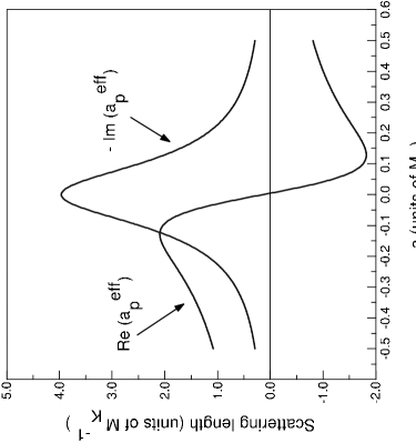
Figure 4: Real and imaginary parts of the complex scattering length $a^{eff}_{p}$ as a function of the parameter $a$ of the isoscalar Bargmann potential. The remaining parameters are as in Table 1. The $f_{0}(980)$ ground state becomes unbound as Re$(a^{eff}_{p})$ passes through zero from positive to negative values.

One can show from Eq. (63) that the sign of Re$(a^{eff}_{I})$ is determined by the sign of the “bare” scattering length $a_{I}$ given by Eq. (25) in the absence of absorption, and hence the sign of the parameter $a$ of the Bargmann potential that controls the existence $(a<0)$ or not $(a>0)$ of a bound state in channel $I$; Im$(a^{eff}_{I})$ is independent of this sign. Fig. 4 illustrates how the real and imaginary parts of $a^{eff}_{p}$ would vary should this parameter vary (i.e. the binding energy vary) in the isoscalar channel. The remaining parameters for this illustration have been kept the same as in Table 1. However, the effects for small variations in the binding energy from real to virtual around zero are not large: for example by simply switching the sign of $a$ to $+0.9136M_{K}$ in Table 1 (thereby also unbinding the isoscalar channel), causes $\sigma_{elas}$ to decrease by $\sim 20\%$ from $106$ to $86$ mb while $\sigma_{a}$ remains unchanged.

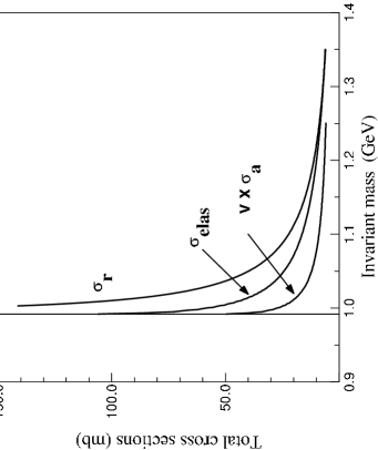
Figure 5: Calculated total $s$–wave elastic, reaction and $v\times$ the annihilation cross sections as a function of the invariant mass $P_{0}$ of the colliding kaon–antikaon pair. The vertical line indicates the threshold value at $2M_{K}$.

Calculations of the total elastic, reaction, and $v$ times the annihilation cross sections based on Eqs. (57) and (58) are shown in Fig. 5. However, as there are as yet no reported measurements of $K\bar{K}$ scattering with which to compare any of these cross sections, we have attempted to use detailed balance to derive the $\pi^{+}\pi^{-}\to K\bar{K}$ cross section, for which measurements do existSDP73 . In this case the latter cross section can be exactly related to the $I=0$ absorption cross section for $K\bar{K}\to\pi\pi$ defined by Eq. (59) as follows (see Eq. (106))

$$p^{2}\sigma_{a}(\pi^{+}\pi^{-}\to K\bar{K})=\frac{2}{3}k^{2}\sigma^{(0)}_{a}=\frac{2\pi}{3}(1-\eta^{2}_{0})$$ (66)

where $\eta_{0}=|S_{0}(k)|$ is the $K\bar{K}$ inelasticity, and where $p$ and $k$ are the relative momenta of the pion or kaon pair of the same total CM energy.

The two curves marked $(a)+(b)$ in Fig. 6 (the upper one includes Coulomb distortionLL58 via the factor $|f^{(-)}_{c}(k,d)|^{-2}\approx 2\pi\eta[exp(2\pi\eta)-1]^{-1}$ taken from Eq. (103) of the Appendix for $kd\sim\mu\alpha d\ll 1$) show the inferred results for $\sigma_{a}(\pi^{+}\pi^{-}\to K\bar{K})$, where they are compared with $\pi^{+}\pi^{-}$ scattering dataSDP73 ; ADM77 , and the fit, curve $(c)$, to these data using a parametrized $\pi\pi$ scattering amplitude with parameters extracted from these experiments. The extraction procedure is documented in detail inSDP73 . A coupled channel treatment of the $\pi\pi$–$K\bar{K}$ system leads to similar resultsLohse90 ; Sassen01 ; julich03 (especially julich03 ) shown by curves $(d)$ and $(e)$.

Fig. 6 clearly shows that the strong enhancement of the cross section near threshold is not adequately reproduced by the pure molecular picture. The same remark holds for the calculated $\pi\pi$ inelasticity, discussed below, that is correspondingly somewhat too large near threshold ( Fig. 7).

The pure molecular picture agrees reasonably well with the result obtained by that coupled channel calculation of julich03 which omits the bare scalar meson state $f_{0}^{\prime}$ (curve $(d)$). This numerical finding justifies the assumptions made in order to obtain a simple analytical model. In order to obtain a good agreement with the data, the introduction of an explicit bare scalar meson state is necessary (curve $(e)$), however.

The parametrized $\pi\pi$ scattering amplitudes as taken from experimentSDP73 (curve (c)) assume the existence of a pole on the second Riemann sheet just below the $K\bar{K}$ threshold at $[997\pm 6-(27\pm 8)i)]$ MeV in the $\pi\pi$ scattering amplitude. The experimentally inferred value of this pole lies reasonably close to the value of the pole on the second sheet for a decaying $f_{0}(980)$ bound state given in Table 2, that has been calculated from the very different points of view presented here and elsewhereWS90 .

A further experimental check on these calculations is provided by comparing with the data BHyams1973 for the $\pi\pi$ isoscalar inelasticity parameter $\eta_{0}(\pi\pi)$. Since we have assumed that only coupling between the $\pi\pi$ and $K\bar{K}$ channels is important, this paramater equals the $K\bar{K}$ inelasticity parameter $\eta_{0}(K\bar{K})=|S_{0}(k)|$ that may be calculated directly from Eq. (60). The resulting prediction for $\eta_{0}(\pi\pi)$ is given in Fig. 7. For comparison we also show the behavior of $\eta_{0}(\pi\pi)$ that follows from a fully relativistic treatment of the pion loop integral under Pauli–Villars regularization with cutoff $\Lambda_{PV}=4$ GeV (the result is rather insensitive to the actual choice of cutoff). There is no difference in the two calculations near threshold. However, the relativistic version becomes more elastic than the non–relativistic calculation with increasing CM energy.

V Kaonium

Besides the isoscalar $K\bar{K}$ bound system, the $K^{+}K^{-}$ component of this state can bind to form a kaonium atom in the long range Coulomb potential. In the following we construct the Jost function that determines the bound states and decay widths of kaonium, that may then be calculated without approximation. The hamiltonian now also includes the Coulomb field $V_{c}=\alpha Q\bar{Q}/r$, ($Q,\bar{Q}$ are particle, antiparticle charge operators) that breaks isospin. However, due to the very disparate length scales $\sim M^{-1}_{K}$ and $\sim(\alpha M_{K})^{-1}$ over which the strong and much weaker Coulomb interactions operate, isospin breaking is essentially confined to that region of space $r\geq d$ outside the range of the strong potential. In this region the wave function reads

$$\frac{1}{r}\Big{(}\varphi_{p}|K^{+}K^{-}>+\varphi_{n}|K^{0}\bar{K}^{0}>\Big{)},\quad r\geq d$$ (67)

where $\varphi_{p}$ and $\varphi_{n}$ describe the $s$–wave radial motion of $K^{+}K^{-}$ and $K^{0}\bar{K}^{0}$ separately in the external region,

$$(\frac{d^{2}}{dr^{2}}+k^{2}-M_{K}V_{c})\varphi_{p}=0,\quad r>d$$

$$(\frac{d^{2}}{dr^{2}}+k^{2})\varphi_{n}=0,\quad r>d$$ (68)

Inside of this range we can ignore isospin breaking entirely due to the dominance of the strong isospin conserving interaction (no internal mixing approximationDR65 ; RHL69 ) and work with states of good isospin. To obtain the Jost function we therefore need to join the linear combinations $-(\varphi_{p}\pm\varphi_{n})/\sqrt{2}$ corresponding to $I=0$ and $1$ in the external region $r\geq d$ onto the known solutions for the complex potentials in Eq. (33) in the internal region $r\leq d$. The latter are given by $\varphi(k,r)$ of Eq. (89) with the appropriate values of $a$, $b$ and $\zeta$ taken from Table 1 for each isospin channel.

For $r>d$ the solution describing the scattering of a $K^{+}K^{-}$ pair is given by the standard expression

$$\varphi_{p}(r)=f^{(-)}_{c}(k,r)-S(k)e^{2i\sigma}f^{(+)}_{c}(k,r)$$ (69)

The $f^{(-)}_{c}(k,r)$ and $f^{(+)}_{c}(k,r)=f^{*(-)}_{c}(k,r)$ represent incoming (outgoing) waves in the Coulomb field, $S(k)$ is the scattering matrix of non–Coulombic origin, $\sigma=arg\Gamma(1+i\eta)$ the Coulomb phase shift and $i\eta=\mu\alpha/ik$ the Coulomb parameter for attractive interactions; $\mu=M_{K}/2$ is the reduced mass. The $f^{(\pm)}_{c}(k,r)$ are proportional to Whittaker functions. One hasRGN66

$$f^{(-)}_{c}(k,r)=e^{\pi\eta/2}W_{i\eta,\frac{1}{2}}(2ikr)$$

$$\approx\frac{e^{\pi\eta/2}}{\Gamma(1-i\eta)}\Big{\{}1-ikr-2\mu\alpha r[\ln 2ikr+\psi(1-i\eta)+2\gamma-1]+\cdots\Big{\}},\quad kr\to 0$$ (70)

where the small $kr$ behavior of $f^{(-)}_{c}(k,r)$ involvesGR80 the standard $\psi$–function, and $\gamma=0.57721$ is the Euler constant.

The $S$–matrix in Eq. (69) is determined by the logarithmic derivative $\zeta_{p}=\varphi^{\prime}_{p}/\varphi_{p}$ of $\varphi_{p}$ at $r=d$. In detail,

$$S(k)=e^{-2i(\sigma-\rho)}\Big{(}\frac{\zeta_{p}-\zeta_{c}}{\zeta_{p}-\zeta^{*}_{c}}\Big{)}$$ (71)

where $\zeta_{c}=f^{\prime(-)}_{c}/f^{(-)}_{c}$ is the logarithmic derivative of the incoming Coulomb wave at $r=d$, and $\rho=\arg f^{(-)}_{c}(k,d)$. Thus the Jost function describing kaonium is proportional to $\zeta_{p}-\zeta_{c}$. To find itRHL69 we determine the value of $\zeta_{p}$ by matching $\varphi_{p}\pm\varphi_{n}$ onto the internal solutions $\varphi_{0}$ and $\varphi_{1}$ of good isospin, where $\varphi_{n}\sim exp(ikr)$ is a pure outgoing wave. Due the large difference in space behavior of the strong $(br\gg 1)$ and Coulombic $(kr\ll 1)$ wave functions near $r\sim d$ for momenta $k\sim\mu\alpha$ of interest for kaonium, the $\varphi(k,r)$ have already reached their asymptotic behavior, while the $f^{(\pm)}_{c}(k,r)$ are still given by their small $kr$ approximation. The matching of value and derivative at $r=d$ is therefore particularly simple to perform. One finds

$$\frac{1}{\zeta_{p}}=\frac{1}{2}\Big{(}\frac{1}{\zeta_{0}}+\frac{1}{\zeta_{1}}\Big{)}$$ (72)

where the logarithmic derivatives $\zeta_{I}=\varphi_{I}^{\prime}/\varphi_{I}$ of the internal wave functions carrying good isospin $I$ are

$$\zeta_{I}=ik\Big{(}\frac{f(k)e^{ikd}+f(-k)e^{-ikd}}{f(k)e^{ikd}-f(-k)e^{-ikd}}\Big{)}_{I}$$ (73)

The eigenvalue condition $\zeta_{p}=\zeta_{c}$ that determines complex energies of kaonium then reads

$$1-\frac{1}{2}\zeta_{c}(\frac{1}{\zeta_{0}}+\frac{1}{\zeta_{1}})=0$$ (74)

This equation contains no free parameters. The Jost functions $f(k)$ in the $\zeta_{I}$ all have pre–determined constants for each isospin channel as given in Table 1, and come from Eq. (35) if annihilation is included, or Eq. (22) if it is not.

It is useful to express the roots of Eq. (74) in the form $k_{\lambda}=-i\lambda\mu\alpha$ since then $\lambda^{-1}\to 1,2,3,...$ for a pure Coulomb field, and also to recognise that the logarithmic derivatives $\zeta_{I}$ can be replaced by their zero momentum values with impunity because $k$ is always ${\cal O}(\mu\alpha)$ for kaonium. Then

$$\frac{1}{\zeta_{I}}\approx-(a^{eff}_{I}-d)+O(1/\zeta^{2})$$ (75)

in terms of the complex scattering length of Eq. (63).

Using these forms for the $\zeta_{I}$, the eigenvalue condition (74) can be reformulated in terms of the complex scattering length $a^{eff}_{p}$ for $K^{+}K^{-}$ scattering as

$$a^{eff}_{p}=\frac{1}{2}(a^{eff}_{0}+a^{eff}_{1})=\Big{(}1-\frac{1}{\zeta_{c}d}\Big{)}d$$ (76)

This leads to an eigenvalue equation of the Kudryavtsev–Popov (KP) typeKP79 ,

$$1/a^{eff}_{p}=2\mu\alpha\Big{[}\psi(1-1/\lambda)+\frac{1}{2}\lambda+\ln(2\lambda\mu\alpha d)+2\gamma\Big{]}$$ (77)

The logarithmic derivative $\zeta_{c}(k)$ of the Coulomb wave function has been calculated at $k_{\lambda}=-i\lambda\mu\alpha$ from Eq. (70).

The resulting complex energy spectrum for kaonium is then given by

$$E_{\lambda}-\frac{i}{2}\Gamma_{\lambda}=-\frac{1}{4}\lambda^{2}M_{K}\alpha^{2}$$ (78)

The solutions of the KP equation are dominated by the $\psi$–function on the right hand side that has poles at $\lambda=1/n$, for integer $n$. These poles just reproduce the pure Coulomb spectrum of kaonium. The strong interaction changes this behavior by moving $\lambda$ off these poles to $\lambda=(n+\delta)^{-1}$, where $\delta$ is complex and not necessarily small. In Table 4 we list a series of exact numerical eigenvalues $\lambda$ of the KP equation, and the associated complex energy spectrum for kaonium. These computations use the value

$$a^{eff}_{p}=(1.940-1.199i)M^{-1}_{K}=(0.77-0.48i){\rm fm}$$ (79)

for the complex scattering length calculated from Eq. (63) plus the data given in Table 3. Notice that the $a_{0}(980)$ admixture introduced via the isovector scattering length $a_{1}$ only contributes to the real part of the $K^{+}K^{-}$ effective scattering length that enters into the calculation of the level shifts and decay widths of kaonium. The imaginary part is entirely determined by the isoscalar piece of the strong interactions. However, due to the non–linear nature of the eigenvalue problem, the isovector contribution nevertheless influences both the real and imaginary parts of the resulting energy spectrum. Only in the perturbative limit (to be described below) does the $a_{0}(980)$ mode contribute solely to the level shifts.

For comparison we have also used the isospin zero and one scattering lengths $\hat{a}^{eff}_{0}=(0.86-1.82i)$ fm and $\hat{a}^{eff}_{1}=(0.06-0.77i)$ fm, based on a recent investigationjulich03 into the effects of a high lying scalar isoscalar quark antiquark configuration (which we refer to as $f_{0}^{\prime}$) mixed into the $K\bar{K}$ molecular ground state. Here the effect of the $\pi\eta$-channel is included too. The $K^{+}K^{-}$ scattering length then becomes

$$\hat{a}^{eff}_{p}=(1.156-3.268i)M^{-1}_{K}=(0.46-1.30i){\rm fm}$$ (80)

instead of Eq. (79).

The predictions for kaonium are given in Tables 4 and 5, while Table 6 summarizes the decrease in lifetime of the ground state as the complexity of the $K^{+}K^{-}$ interaction is increased. In particular, Table VI shows that the lifetime of kaonium is reduced further by about a factor of three once annihilation in the isovector channel is introduced via the $\pi\eta$ decay of the $a_{0}(980)$. These results are qualitatively similar to those given by other approaches to the problem of kaonium formation and decaySWycech . One notes from Tables 4 and 5 that Re$\lambda<1/n$, corresponding to a positive shift of the Coulomb level when the strong interaction supports a bound state (the sign of the real part of the scattering length determines the sign of the level shift). In addition to causing repulsive shifts of the Coulomb levels the strong field introduces a decay width due to $K^{+}K^{-}\to 2\pi$ annihilation with a lifetime of $\sim 10^{-18}$ sec (the two–photon annihilation lifetime at ${\cal O}(M^{-1}_{K}\alpha^{-5})\sim 10^{-13}$ sec, or one in $10^{5}$ decays, is too long to compete). It also introduces an extra node into all the eigenfunctions of kaonium. This means that the kaonium levels represent excited states in the combined Coulomb plus strong fields of the $K\bar{K}$ system. As will be discussed in more detail below, the occurrence of this node is responsible for making the kaonium lifetime two orders of magnitude shorter than the $\sim 10^{-16}$ sec it would have been had the $K^{+}K^{-}$ pair only been bound by a Coulomb field.

Let us briefly indicate how these features come about. The appearance of the additional radial node is required by the fact that the $1s$ state of relative motion has been usurped by the $K\bar{K}$ ground state in the strong potential. So the ground and excited levels of kaonium have to have a $2s,3s...$ character with one additional node. This node is always positioned in the close proximity of the $K^{+}K^{-}$ scattering length, independent of the excitation energy. It is real or virtual depending on whether the strong interaction supports a real ($a_{p}>0$) or a virtual ($a_{p}<0$) bound state. This comes about as follows. The kaonium levels are all weakly bound at $k\sim\mu\alpha$ so that their radial wave functions in the inner region all become nearly identical with the zero energy wave functions of $K\bar{K}$ in the strong potential alone. These functions [see Eq. (99)] all have a node at $r=a_{p}$ in the effective range approximation. The remaining nodes are supplied by the Whittaker function $W_{1/\lambda,\frac{1}{2}}(2\lambda\mu\alpha r)$ in the external region, $r\geq d$. They are almost identical with those of a pure Coulomb field bound state wave function where $\lambda=1/n$.

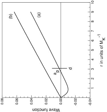
Figure 8: Kaonium ground state radial wave functions: (a) with and (b) without the meson exchange fields present. In (a) the strong field solution, Eq. (97), is joined smoothly at $r=d$ onto the Whittaker function $W_{1/\lambda,\frac{1}{2}}(2\lambda\mu\alpha r)$ for $\lambda=0.981$. The node in this solution falls at the $K^{+}K^{-}$ scattering length $a_{p}$. In (b) the solution $W_{1,\frac{1}{2}}(2\mu\alpha r)=2\mu\alpha r\>\exp{(-\mu\alpha r)}$ for a pure Coulomb field, $\lambda=1$, is plotted for the same range of $r$. To set the scale, note that the Bohr radius of kaonium would fall at $\sim 300$ units to the right of this figure.

The eigenfunction for the lowest state of kaonium is illustrated in Fig. 8 (with absorption suppressed). It is clear from this figure that the actual choice of the cutoff $d$ is immaterial if taken anywhere in the region where the wave function behaves linearly. A closed form for the bound state eigenfunctions $\varphi_{1/\lambda}$ of kaonium labelled by the quantum number $\lambda^{-1}$ is given in Eq. (97) in the Appendix. From that one calculates that the gradient at the origin is enhanced by the factor $b/a$ in both isospin channels over that of the pure Coulomb state. Physically this comes about because the strong potentials draw the $K^{+}K^{-}$ pair much closer together, thereby increasing the probability density of finding them at the origin by $(b^{2}/a^{2})_{I}$ (notice $b>|a|$ from Eq. (26)) in each isospin component, where they annihilate. In the isoscalar channel, which is strongly attractive, the effect is especially marked, $(b^{2}/a^{2})_{0}\sim 60$. On the other hand the isovector channel only supports a virtual state. Hence the concentration of probability density at the origin in this channel is much weaker, $(b^{2}/a^{2})_{1}\sim 3$.

The effect of this factor in the isoscalar channel is quite dramatic. It increases the decay width of kaonium by two orders of magnitude (with a corresponding decrease in lifetime) over what it would have been in the absence of the strong potentials $V_{I}$. One can illustrate this qualitatively by appealing to the perturbative solutionKP79 ; Deser54 of the KP equation for the complex energy shift. For the ground state this reads

$$\Delta E-\frac{i}{2}\Gamma\approx\frac{1}{2}M^{2}_{K}\alpha^{3}a^{eff}_{p}=\frac{1}{2}M^{2}_{K}\alpha^{3}a_{p}-\frac{1}{2}M^{2}_{K}\alpha^{3}\xi^{-1}\big{[}\frac{1}{2}(\frac{b^{2}}{a^{2}})_{0}\big{]}$$ (81)

that equals either $(0.187-0.116i)$ keV, or $(0.187-0.164i)$ keV depending on whether the value (79) or its low absorption version $\xi\gg 1$ taken from Eq. (63),

$$a^{eff}_{p}\approx\frac{(a_{0}+a_{1})}{2}-\frac{i}{2}(\frac{b^{2}}{a^{2}\xi})_{0}=(1.940-1.703)M^{-1}_{K}$$ (82)

is used for the effective scattering length. The $a_{I}$ are the bare scattering lengths of Eq. (25) as before. The last approximation places the role of the isoscalar probability density admixture $(b^{2}/a^{2})_{0}$ in the kaonium ground state explicity in evidence.

Neither approximation is very accurate in comparison with the exact solution of $(0.181-0.107i)$ keV, but can be used to illustrate the effect of strong interactions decreasing the lifetime of kaonium against what it would have been in a pure Coulomb field. One sees this as follows. The decay width in Eq. (81) is directly related to the “annihilation at rest” cross section

$$\sigma_{a}\approx-\frac{4\pi}{k}Im(a^{eff}_{p})=\frac{4\pi}{k}\frac{1}{2}\big{[}\frac{b^{2}\xi}{a^{2}\xi^{2}+(b^{2}-a^{2})^{2}}\big{]}_{0}\approx\frac{4\pi}{k\xi}\big{[}\frac{1}{2}(\frac{b^{2}}{a^{2}})_{0}\big{]}$$ (83)

as $\Gamma=v\phi^{2}(0)\sigma_{a}$, upon multiplication by the flux factor $v\times\phi^{2}(0)$ where $\phi^{2}(0)=M^{3}_{K}\alpha^{3}/8\pi$ gives the probability per unit volume for finding the $K^{+}K^{-}$ pair at the origin when bound by the Coulomb field alone; $v=k/\mu$ is their relative velocity. On the other hand when the strong potential is absent, the scattering lengths $a^{eff}_{0}\to-i/\xi$ and $a^{eff}_{1}\to 0$ are pure imaginary and zero respectively, so that $a^{eff}_{p}\to-i/2\xi=-0.028iM^{-1}_{K}$, and the corresponding free annihilation cross section becomes

$$\sigma_{a,free}=\frac{4\pi}{k\xi}(\frac{1}{2})\approx\sigma_{a}/\theta,\quad\theta\sim 42\;{\rm to}\;60$$ (84)

if we use the unexpanded or expanded version of $\sigma_{a}$ in Eq. (83). The factor $\theta$ reflects the modification of the kaonium ground state due to the strong interactions.

In this case there is no energy shift at all, and the decay half–width is $\frac{1}{2}\Gamma_{free}=0.0028$ keV, leading to a lifetime of $\tau_{free}=1.2\times 10^{-16}$ sec. So the $K^{+}K^{-}\to 2\pi$ strong potential assisted annihilation lifetime drops by roughly the factor $\theta$ from $1.2\times 10^{-16}$ sec that it would have been in a pure Coulomb field, to $3.2\times 10^{-18}$ sec as given by the exact solution of the KP equation. Table 6 summarizes the change in lifetime of the kaonium ground state as the complexity of the $K^{+}K^{-}$ interaction changes from assuming free annihilation at rest in a Coulomb field, to including one–boson exchange, to adding $f^{\prime}_{0}$ mixing, for determining the scattering length.

We note in passing from the center expression for $\sigma_{a}$ in Eq. (83) that if the bound state occurs at zero energy ($a=0$), the corresponding enhancement of the annihilation width is maximal. Also, while generally true of the exact solutions of the KP equation, the perturbative solution given in Eq. (81) makes it evident that the sign of the level shift goes along with the sign of the scattering length, which is positive for bound and negative for unbound or virtual states.

We close this section with a comment on to what extent the results for kaonium might be considered as ”parameter–free”. Apart from specifying a Lagrangian with the attendant assumption of $SU(3)$ symmetry that fixes the various coupling constants in terms of $g_{\rho\pi\pi}$, that we in turn fixed from the KSRF relation, the only arbitrary parameter in these calculations was the form factor cutoff $\Lambda$ introduced in Section IIIA. The choice $\Lambda=4$ GeV, that was also used in Ref. Lohse90 , led to calculated scattering lengths and effective ranges for the $K\bar{K}$ system, that were then duplicated by constructing an equivalent Bargmann potential that depended on two parameters $a$ and $b$. This in turn gave predictions for the mass and width of a bound $K\bar{K}$ molecular state in reasonable accord with the known experimental mass and width of the $f_{0}(980)$ scalar meson. However, as already demonstrated in Table 2, one can turn the argument around without materially affecting any of our conclusions for kaonium, by asserting that the Bargmann parameters $a$ and $b$ are actually pre–determined from experiment in the strong interaction sector, thus leaving the kaonium sector without any free parameters at all.

Similar remarks hold true for the calculated cross sections shown in Figs. 5 and 6. Once $a$ and $b$ have been fixed from experiment or otherwise, no further adjustable parameters enter into these calculations. The actual values of $a$ and $b$ as determined by any of the five alternatives shown in Table 2 do not in fact differ very much.

VI Discussion

In this investigation we have shown that one meson exchange potentials derived from a standard $SU(3)_{V}\times SU(3)_{A}$ Lagrangian in the non–relativistic limit are sufficient to bind $K\bar{K}$ into a kaonic molecule with a mass and decay width that closely match the experimental values of the $f_{0}(980)$ isoscalar meson. We have also shown that the same potentials, in combination with detailed balance, lead to a prediction of the $\pi^{+}\pi^{-}\to K\bar{K}$ cross section that is too low especially near threshold.

We have further demonstrated that there are specific, experimentally observable effects in the energy level shifts and decay properties of the kaonium spectrum, in the presence of a $K\bar{K}$ molecular ground state. The existence of such a bound $K\bar{K}$ pair would be reflected in positive energy level shifts in the kaonium Coulomb spectrum (due to level repulsion), plus enhanced $K^{+}K^{-}\to 2\pi$ decay widths. On the other hand, unbound or virtually bound (and therefore weakly correlated) $K\bar{K}$ pairs produce negative energy level shifts and a weak enhancement of the decay widths. Since the sign of the level shifts and the enhancement of the decay widths go together with the presence or absence of a strongly correlated $K\bar{K}$ pair in the ground state, measurements of the level shifts and decay widths in kaonium could provide another probe for investigating to what extent the $f_{0}(980)$ meson ground state has a $K\bar{K}$ molecular component. From the experimental point of view it is important to stress that, as for protoniumKP79 which has a very similar decay width, the $1s-2s$ level spacing of $\sim 5.1$keV in kaonium is many times the estimated decay widths $\lesssim 200$ eV, so that these levels remain distinguishable in the presence of the $2\pi$ decay channel.

Notwithstanding the results reported in Barnes1985 , we again stress the conflict that exists between the pure molecular description of the $f_{0}(980)$ ground state and the calculated $2\gamma$ decay width. In Barnes1985 a binding energy of $10$ MeV for the kaonium molecule was assumed, that leads to a width of $\sim 0.6$ keV. However, most recent data show a resonance energy that corresponds to a pole in the complex plane, which translates into a binding energy of $18$ to $20$ MeV for the molecular potential. This increase in binding energy enhances the value of the spatial wave function at the origin by a factor of three, see Fig. 11. One way of understanding the origin of this discrepancy is to generalise the molecular picture of the $f_{0}(980)$ to a superposition of a $K\bar{K}$ component and a hard component. In the Jülich model Lohse90 a $f^{\prime}_{0}$ state has been considered in addition to the pure molecule in order to reproduce the large inelasticities of the $\pi\pi$ phase shifts in the vicinity of the $K\bar{K}$ threshold. The $f^{\prime}_{0}$ state may be interpreted as either a $q\bar{q}$ or as a $q^{2}\bar{q}^{2}$ configuration. As pointed out by Achasovachasov82 and confirmed by current algebraRHLRT2002 , the large decay width of the former into two pions may disqualify a $q\bar{q}$ interpretation of the additional component $f^{\prime}_{0}$. The effect of the $f^{\prime}_{0}$ component in the $f_{0}(980)$ meson introduced in the Jülich model is to reduce the lifetime of kaonium from $3.2\times 10^{-18}$ sec to $1.1\times 10^{-18}$ sec. The presently available data concerning the inelasticities of the $\pi\pi$ phase shifts, and in particular the $\pi^{+}\pi^{-}\to K\bar{K}$ cross sections, do not allow one to disentangle the components of the $f_{0}(980)$ structure in a model independent way. High resolution data for two kaon production near to the threshold will be undertaken at COSY in the near future.

VII Acknowledgements

One of us (RHL) would like to thank Prof. Speth of the Institut für Kernphysik Theory Division, Forschungszentrum, Jülich, for the exceptional hospitality of the institute, and for financial support. It is a pleasure to thank M. Büscher, D. Gotta, C. Hanhart and A. E.Kudryavtsev for useful discussions.

*

Appendix A

A.1 Isospin phase conventions

In order to construct two–meson states of good isospin using conventional Clebsch–Gordan coefficients the following phase conventions are useful.

If one choosesPetersen71 as basis states $|\pi^{\pm}>=\mp|\pi,\pm 1>$, and $|\pi^{0}>=|\pi,0>$ for charged and neutral pions, the two–pion state of good isospin $|I=0,I_{3}=0>$ is, for example,

$$|(\pi\pi)_{0}>=-\sqrt{\frac{1}{3}}\Big{[}|\pi^{+}(1)\pi^{-}(2)>+|\pi^{-}(1)\pi^{+}(2)>+|\pi^{0}(1)\pi^{0}(2)>\Big{]}$$ (85)

Since the pions are identical bosons in the isospin basis, one has to include a space part of the two–pion wave function that is symmetric in particle label interchange to accompany $|I=0,I_{3}=0>$. The normalization of the symmetrized product of the two–pion space wave function introduces an additional factor $n_{s}=1/\sqrt{2}$.

For the kaon and anti–kaon isospin doublet and anti–doublet the analogous convention is, in matrix form,

$$K=\left(\begin{array}[]{c}K^{+}\\ K^{0}\\ \end{array}\right),\quad\bar{K}=\left(\begin{array}[]{c}\bar{K}^{0}\\ -K^{-}\\ \end{array}\right)$$

Consequently the isoscalar and isovector combinations $|I=0,I_{3}=0>$ and $|I=1,I_{3}=0>$ are

$$|(K\bar{K})_{0}>=-\frac{1}{\sqrt{2}}[|K^{+}(1)K^{-}(2)>+|K^{0}(1)\bar{K}^{0}(2)>]$$

$$|(K\bar{K})_{1}>=-\frac{1}{\sqrt{2}}[|K^{+}(1)K^{-}(2)>-|K^{0}(1)\bar{K}^{0}(2)>]$$ (86)

These relations lead immediately to the values of the isospin coefficients $C_{I}$ and $n_{s}$ quoted below Eq. (13) in the text.

A.2 Wave functions for the Bargmann potentials

We briefly summarize some results of Bargmann for constructing phase equivalent potentials. As shown inBargmann49 the assumed form Eq. (22) for the Jost function gives rise to a family of potentials that lead to this form for $f(k)$: the simplest one of this family is given by Eq. (23). Let $\psi(r)=r^{-1}\varphi(r)$, and replace the OBE potentials by this form for $V_{I}$. Then

$$\varphi^{\prime\prime}+(k^{2}-M_{K}V_{I})\varphi=0$$ (87)

for $K\bar{K}$ $s$–wave scattering. The two linearly independent solutions $f(\pm k,r)$ for this equation that are irregular at the origin are known in closed form by constructionBargmann49 ; Newton60

$$f(k,r) =e^{-ikr}\frac{k-ib[b\sinh(br)+a\cosh(br)][b\cosh(br)+a\sinh(br)]^{-1}}{k-ib}$$ (88)

$$\to e^{-ikr},\quad r\to\infty$$

A general solution of Eq. (87) can be written as a linear combination of the $f(\pm k,r)$,

$$\varphi(k,r)=\frac{i}{2k}[f(-k)f(k,r)-f(k)f(-k,r)]$$ (89)

where the coefficient $f(k)$ is the Jost function. It can be shown quite generallyNewton60 that $f(k)$ is determined by the Wronskian of $f(k,r)$ and $\varphi(k,r)$:

$$f(k)=W[f(k,r),\varphi(k,r)]=[f\varphi^{\prime}-f^{\prime}\varphi]$$ (90)

Since $W$ is independent of $r$ this can be evaluated at any convenient point, in particular at the origin. The value of $f(k)$ is determined by how $\varphi$ behaves at the origin. If $\varphi\sim r$, then $f(k)=f(k,0)=(k-ia)/(k-ib)$ as in Eq. (22). This is the usual case. On the other hand if $\varphi$ does not vanish at the origin, but instead possess a finite logarithmic derivative there, then $f(k)$ is given by Eq. (35).

In the first case one obtains the usual scattering solution of Eq. (87) that vanishes at the origin as

$$\varphi(k,r) =\frac{\sin kr}{k}+\frac{b^{2}-a^{2}}{b^{2}+k^{2}}\frac{1}{k}\frac{k\sinh(br)\cos(kr)-b\cosh(br)\sin(kr)}{a\sinh(br)+b\cosh(br)}$$ (91)

If $a=-\kappa$ is negative, then $f(k)$ has a zero in the lower half of the complex $k$-plane, corresponding to a bound state with binding energy $\varepsilon=\kappa^{2}/M_{K}$. The associated bound state wave function is found by setting $a=-\kappa$ and $k=-i\kappa$ in Eq. (91) to find

$$\varphi(-i\kappa,r) =\frac{\sinh(br)}{b\cosh(br)-\kappa\sinh(br)}e^{-\kappa r}$$ (92)

The normalization of this bound state is also available from a knowledge of the Jost function:

$$\int_{0}^{\infty}dr\varphi^{2}(-i\kappa,r)=\frac{i}{4\kappa^{2}}f(i\kappa)\frac{\partial f(k)}{\partial k}_{k\to-i\kappa}=\frac{i}{4\kappa^{2}}f(i\kappa)\dot{f}(-i\kappa)=\frac{1}{2\kappa(b^{2}-\kappa^{2})}$$ (93)

since $f(k)=(k+i\kappa)/(k-ib)$. The normalized bound state is then given by

$$\psi(r)=(\sqrt{4\pi}r)^{-1}\sqrt{2\kappa(b^{2}-\kappa^{2})}\frac{\sinh(br)}{b\cosh(br)-\kappa\sinh(br)}e^{-\kappa r}$$ (94)

In Fig. 11 we compare the radial eigenfunction as obtained by numerically solving for the $K\bar{K}$ isoscalar bound state in the one boson exchange potential of Eq. (17), with the analytical solution given by Eq. (94) for the phase equivalent Bargmann potential. Except in the vicinity of the origin, where the numerical solution is underestimated by a factor $\sim 1.2$, the two wave functions are essentially identical. Also shown is the wave function at $10\textrm{ MeV}$ binding in a gaussian potential that was used in Barnes1985 to estimate $\psi(0)$.

Finally in Fig. 12 we illustrate the variation of the spatial wave function $\psi(0)$ of Eq. (94) as a function of its binding energy. This plot was obtained by using the calculated variation of $a_{0}$, $r_{0}$ and $\varepsilon$ with cutoff as shown in Fig. 2 for the one boson exchange potential to obtain the parameters $a=-\kappa$ and $b$ at each binding energy.

The inclusion of the annihilation potential changes the solution for the radial eigenfunction from $\varphi(-i\kappa,r)$ to the complex solution

$$\tilde{\varphi}(k_{r},r)=f(k_{r},r)/f(k_{r},0)\quad$$ (95)

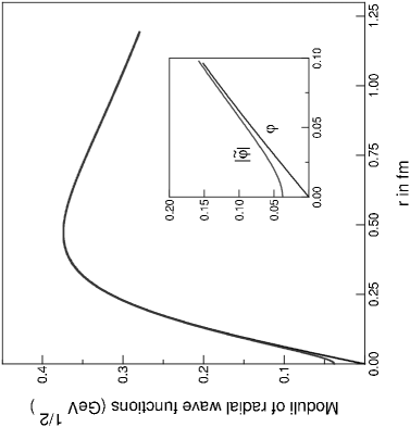
Figure 9: A plot of (the moduli of) the normalized radial wave functions $\tilde{\varphi}(k_{r},r)$ and $\varphi(-i\kappa,r)$ that include and exclude annihilation effects respectively. The inset details their behavior for small $r$. Notice that $|\tilde{\varphi}(k_{r},r)|$ “heals” to $\varphi(-i\kappa,r)$ within $0.1$ fm away from the origin.

where $k_{r}=(0.1254-0.1972i)M_{K}$ is the root of the Jost function in the presence of annihilation as given by Eq. (50). One readily verifies that $\tilde{\varphi}(k_{r},0)=1$ and $\tilde{\varphi}^{\prime}(k_{r},0)=\zeta=-i\xi$ as required. A comparative plot of the normalized versions of the moduli of $\tilde{\varphi}(k_{r},r)$ and $\varphi(-i\kappa,r)$ is given in Fig. 9. Since the derivative of $\tilde{\varphi}(k_{r},r)$ at the origin is purely imaginary, its modulus has a zero derivative there. This is clearly visible in the inset in Fig. 9, that also shows how $|\tilde{\varphi}(k_{r},r)|$ “heals” within $0.1$ fm away from the origin from the effects of the annihilation potential to rejoin the real solution $\varphi(-i\kappa,r)$. Either eigenfunction leads to a rms molecular radius of $\sqrt{<r^{2}>}\approx 1.62$ fm, (i.e. about two proton charge radii).

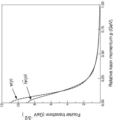
Figure 10: Normalized fourier transforms of the spatial wave functions $\tilde{\psi}(r)$ with and $\psi(r)$ without annihilation.

The momentum content of the normalized spatial wave functions $\psi(r)=(\sqrt{4\pi}r)^{-1}\varphi(-i\kappa,r)$ and $\tilde{\psi}(r)=(\sqrt{4\pi}r)^{-1}\tilde{\varphi}(k_{r},r)$ is given by their fourier transforms $\psi(p)$ and $\tilde{\psi}(p)$. These are shown in Fig. 10 for relative meson momenta up to $1$ GeV. As expected from Fig. 9, the effect of the annihilation potential is to redistribute the momentum to higher values, while at the same time leaving the characteristic value of $<p^{2}>$ at $\sim 0.08$ GeV² for the relative meson momentum squared in the molecule.

A.3 Matching of isospin amplitudes

The wave functions of kaonium in the inner, or isospin conserving region are given by Eq. (89). These solutions either vanish at the origin, or possess a given logarithmic there, depending on the form of $f(k)$ that is chosen. Matching either form onto the linear combinations $\varphi\pm\varphi_{n}$ of the outside solutions at $r=d$, one finds the consistency condition

$$\left(\begin{array}[]{cc}\zeta_{0}-\zeta_{p}&\zeta_{0}-\zeta_{n}\\ \zeta_{1}-\zeta_{p}&-\zeta_{1}+\zeta_{n}\\ \end{array}\right)\left(\begin{array}[]{c}\varphi_{p}\\ \varphi_{n}\\ \end{array}\right)=0$$

where $\zeta_{n}=\varphi_{n}^{\prime}/\varphi_{n}$. The other logarithmic derivatives have been defined in the main text. At momenta $k\sim\mu\alpha$ of relevance for kaonium, $\zeta_{n}=ik$ is much smaller than any of these so we simply drop it and find

$$\frac{1}{\zeta_{p}}\approx\frac{1}{2}\big{(}\frac{1}{\zeta_{0}}+\frac{1}{\zeta_{1}}\big{)};\quad\varphi_{n}/\varphi_{p}\approx-1+\zeta_{p}/\zeta_{0}=1-\zeta_{p}/\zeta_{1}$$ (96)

The eigenvalue condition $\zeta_{p}=\zeta_{c}$ determines the values of $k=-i\kappa$, which are pure imaginary in the absence of absorption, for the bound states of kaonium, and at the same time removes the outgoing wave piece of $\varphi_{p}$ from Eq. (69). Then the matching conditions show that the kaonium eigenfunctions that join smoothly onto the pure decaying state $f^{(-)}_{c}(-i\kappa r)\sim W_{1/\lambda,\frac{1}{2}}(2\kappa r)$ outside the strong potential are given by a linear combination of isospin zero and one internal functions as

$$\varphi_{1/\lambda}(r) =\frac{1}{2}\zeta_{c}f_{c}\Big{[}\frac{1}{\zeta_{0}}\frac{\varphi_{0}(-i\kappa,r)}{\varphi_{0}(-i\kappa,d)}+\frac{1}{\zeta_{1}}\frac{\varphi_{1}(-i\kappa,r)}{\varphi_{1}(-i\kappa,d)}\Big{]},\quad r\leq d$$ (97)

$$=f_{c}(-i\kappa,r),\quad r\geq d$$

where $\zeta_{c}=\zeta_{c}(-i\kappa)$ and $f_{c}=f^{(-)}_{c}(-i\kappa,d)$. We have labelled these eigenfunctions with the “quantum number” $\lambda^{-1}=\mu\alpha/\kappa$ that reverts to an integer for a pure Coulomb field. One verifies immediately that the matching of value at $r=d$ is guaranteed by the eigenvalue condition (74) or (96), while the derivatives match identically from the definition of the logarithmic derivatives.

These eigenfunctions develop a common additional node at the $K^{+}K^{-}$ scattering length, independent of the energy of the kaonium level. Consider the case where the scattering length is real. Then this happens because $\kappa\sim\mu\alpha\ll M_{K}$ is very small so that the behavior of the $\varphi_{I}(-i\kappa,r)$ differ but little from their zero energy behavior. From Eq. (91) this is

$$\varphi(0,r) =\frac{b-a}{b^{2}}\Big{\{}\frac{(b+a)\sinh(br)}{b\cosh(br)+a\sinh(br)}+r\frac{ba}{b-a}\frac{b\sinh(br)+a\cosh(br)}{b\cosh(br)+a\sinh(br)}\Big{\}}$$ (98)

$$\sim r,\quad br\ll 1$$

$$\sim\frac{a}{b}(r-a_{I}),\quad br\gg 1$$

where $a$ and $b$ refer to channel $I$. Inserting this information into Eq. (97), one finds that

$$\varphi_{1/\lambda}\sim-(\zeta_{c}a_{p})f_{c}(1-r/a_{p})$$ (99)

outside the range of the strong interaction.

We return to the neglect of the $K^{0}$–$K^{\pm}$ mass difference $\Delta$ in calculating the logarithmic derivative $\zeta_{n}$ for the $K^{0}\bar{K}^{0}$ channel. Including $\zeta_{n}=-\sqrt{2M_{K}\Delta}$ leads to a revised version of the eigenvalue equation (74) that now reads

$$1-\frac{1}{2}(\zeta_{c}+\zeta_{n})\big{(}\frac{1}{\zeta_{0}}+\frac{1}{\zeta_{1}}\big{)}+\frac{\zeta_{c}\zeta_{n}}{\zeta_{0}\zeta_{1}}=0$$ (100)

The lowest eigenvalue of this equation is $\lambda=0.9860+0.0061i$ instead of $0.9863+0.0082i$, an inessential change. The reason is the dominating influence of the isoscalar channel for which $\zeta_{0}d\approx 18.0-10.5i$, that overshadows the remaining logarithmic derivatives, which are all ${\cal O}(1)$, and suppresses the last term in Eq. (100).

A.4 Coulomb distortion

It is also useful to document the modification due to the Coulomb interaction on the low–momentum behavior of the absorption cross section as given by the second of Eqs. (65). Using Eqs. (71), (72) and (75), one finds that

$$\sigma_{a}\approx\frac{4\pi}{k^{2}}Im(a^{eff}_{p})Im(\zeta_{c})\approx-\frac{4\pi}{k}\frac{Im(a^{eff}_{p})}{|f^{(-)}_{c}(k,d)|^{2}}$$ (101)

since $Im(\zeta_{c})=-k|f^{(-)}_{c}(k,d)|^{-2}$ is the imaginary part of the logarithmic derivative $\zeta_{c}$ of the incoming Coulomb wave. The latter relation is easily found by writing $f^{(-)}_{c}(k,r)={\rm exp}(i\sigma)(G(k,r)-iF(k,r))$ in terms of the regular and irregular Coulomb solutions $F(k,r)\sim\sin(kr-\eta\ln 2kr+\sigma)$, $G(k,r)\sim\cos(kr-\eta\ln 2kr+\sigma)$, so that

$$\zeta_{c}=\Big{(}\frac{GG^{\prime}+FF^{\prime}-ik}{G^{2}+F^{2}}\Big{)}_{r=d}$$ (102)

after using the Wronskian relation $(GF^{\prime}-G^{\prime}F)=k$ that holds for all $r$. For $kd\sim\mu\alpha d<<1$ one finds from Eq. (70) that

$$|f_{c}^{(-)}(k,d)|^{2} =\Big{(}\frac{e^{2\pi\eta}-1}{2\pi\eta}\Big{)}\Big{[}\Big{(}1-2\mu\alpha d(\ln 2\mu\alpha d+2\gamma-1)\Big{)}^{2}+\Big{(}\frac{2\pi\mu\alpha d}{(e^{2\pi\eta}-1)}\Big{)}^{2}\Big{]}$$ (103)

$$\sim\Big{(}\frac{e^{2\pi\eta}-1}{2\pi\eta}\Big{)},\quad\eta=-\mu\alpha/k$$

in agreement with Ref. LL58 .

A.5 Detailed balance

If one ignores the real one–boson exchange potential $V_{I}$ in Eq. (33), then the Jost function for $K\bar{K}$ scattering due to the annihilation part alone is simply $f(k)=\zeta+ik$. This gives rise to a $s$–wave $I=0$ scattering length of

$$4\pi a_{0}(K\bar{K})=-M_{K}c^{2}_{0}$$ (104)

after using the definition (34) for $\zeta$. However, since $\pi\pi$ annihilation into $K\bar{K}$ is described by the same diagram in Fig. 3 with the pion and kaon lines interchanged, the $I=0,\;\pi\pi$ scattering length due to this process alone is also given to the same approximation by the expression as above, but with $M_{\pi}$ and $M_{K}$ interchanged in the product $M_{K}c^{2}_{0}$, i.e.

$$4\pi a_{0}(\pi\pi)=-[M_{K}c^{2}_{0}]_{M_{\pi}\leftrightarrow M_{K}}=-\frac{k}{p}M_{K}c^{2}_{0}=4\pi a_{0}(K\bar{K})\left(\frac{k}{p}\right)$$ (105)

We have used Eq. (31) to perform the mass interchange. Here $p$ and $k$ are the relative momenta of a pion or kaon pair with the same total CM energy $P_{0}$. There is no contribution to the $a_{2}(\pi\pi)$ scattering length from Fig. 3 in the $I=2$ channel, since the intermediate kaon loop can at most carry $I=1$. Consequently detailed balance holds between the $I=0$ absorption cross section $\sigma^{(0)}_{a}(\pi\pi\to K\bar{K})$ and its inverse $\sigma^{(0)}_{a}(K\bar{K}\to\pi\pi)$ when viewed in the isospin basis under the above approximations.

However the physical $\pi^{+}\pi^{-}$ channel is described by the scattering length $a(\pi^{+}\pi^{-})=\frac{2}{3}a_{0}(\pi\pi)+\frac{1}{3}a_{2}(\pi\pi)$. But $Im\big{(}a_{2}(\pi\pi)\big{)}=0$, so

$$\sigma_{a}(\pi^{+}\pi^{-}\to K\bar{K})=-\frac{4\pi}{p}Im\left(\frac{2}{3}a_{0}(\pi\pi)\right)=\frac{2}{3}\frac{k^{2}}{p^{2}}\sigma^{(0)}_{a}(K\bar{K}\to\pi\pi)$$ (106)

provided that $P_{0}\geq 2M_{K}$.

A.6 Dimensional regularization of $J(P_{0})$

Replace the three–dimensional integral in Eq. (29) by its analog in $d$ dimensionsGLRG01 ,

$$J(P_{0}) =\int\frac{d^{3}{\bf l}}{(2\pi)^{3}}\Big{(}\frac{1}{{\bf l^{2}}/M+2M-P_{0}}\Big{)}\to\frac{1}{(4\pi)^{d/2}}\frac{1}{\Gamma(d/2)}\int_{0}^{\infty}dL^{2}\frac{(L^{2})^{d/2-1}}{L^{2}/M+2M-P_{0}}$$ (107)

$$=\Big{[}M(2M-P_{0})\Big{]}^{d/2-1}\frac{M}{(4\pi)^{d/2}}\Gamma[1-d/2]$$

or, as $d\to 3$,

$$J(P_{0})=-\frac{M}{4\pi}\Big{[}M(2M-P_{0}\Big{]}^{1/2}=\frac{M}{4\pi}\Big{[}M|(P_{0}-2M)|\Big{]}^{1/2}e^{i(\phi+\pi)/2}\quad 0<\phi<2\pi\quad JP$$ (108)

on the first sheet of the complex $P_{0}$ plane. Note that $J(P_{0})$ is pure imaginary and positive on the upper lip of the cut $\phi=0$ extending from $2M$ to $\infty$. The analytic continuation to the second sheet through the cut starting at the branch point $P_{0}=2M$ is obtained by taking $-2\pi<\phi<0$.

Figure 3: Replacement of the irreducible $K\bar{K}$ scattering diagram involving the exchange of two $K^{*}$’s by an equivalent pion loop diagram with point vertices.

Figure 6: The $\pi^{+}\pi^{-}\to K\bar{K}$ cross section given by detailed balance, Eq. (66), as a function of the $K\bar{K}$ invariant mass $P_{0}$. The two curves designated (a)+(b) give the results with (upper curve) and without (lower curve) Coulomb distortion. Also shown are the $\pi^{+}\pi^{-}\to K\bar{K}$ experimental dataSDP73 (closed circles), and ADM77 (crosses). Curve (c)) is a fit to these data using the parametrized scattering matrix of SDP73 . Curves $(d)$ and $(e)$ correspond to coupled channel calculations of the $\pi^{+}\pi^{-}\rightarrow K\bar{K}$ cross section with (curve $(e)$) and without (curve $(d)$) $f_{0}^{\prime}$ mixing.

Figure 7: The $\pi\pi$ inelasticity parameter $\eta_{0}(\pi\pi)$ as a function of the CM energy. The experimental data is taken from BHyams1973 . The upper curve shows the behavior of the inelasticity given by a fully relativistic calculation of the pion loop integral.

Figure 11: Comparison of the bound state wave function obtained numerically (curve $(a)$) for the isoscalar one boson exchange potential of Eq. (17), with that given by the analytical solution, Eq. (94), for the equivalent Bargmann potential (curve $(b)$). Curve $(c)$ shows the wave function in a gaussian potential adjusted to give a binding energy of $10\textrm{ MeV}$ Barnes1985 .

Figure 12: Variation of the spatial wave function $\psi(0)$, Eq. (94), with binding energy.

Table 1: Parameters of the Bargmann potentials, Eq. (23), that give rise to identical scattering lengths and effective ranges as the one boson exchange potentials in Eqs. (17) and (18). The last column gives the value of the logarithmic derivative that determines the strength the annihilation potential. The units are $M_{K}$.

Isospin	$a$	$b$	$\zeta$
$I=0$	$-0.1936$	$1.491$	$-17.409i$
$I=1$	$+0.9219$	$1.462$	$-26.114i$

Table 2: Summary of calculated isoscalar $K\bar{K}$ scattering lengths $a^{\prime}_{0}$ and effective ranges $r^{\prime}_{0}$ (in units $M^{-1}_{K}$), based on the $a$ and $b$ Bargmann potential parameters (in units $M_{K}$) that reproduce the complex bound state at $P_{0}$ shown in column two. The physical constants that enter into these calculations are: $(M_{\pi},M_{K},M_{K^{*}})=(140,496,892)$ MeV, and $\alpha_{s}=g^{2}_{\rho\pi\pi}/4\pi\approx 2.9$, using the KSRF value of $g_{\rho\pi\pi}\approx 6$. The last four rows list the values of $a$ and $b$, and the resulting isoscalar scattering lengths and effective ranges that would be required to reproduce the theoretical results of Weinstein and Isgur (WI), the fits of Morgan and Pennington (MP), and the experimental data.

Source	$P_{0}=M-i\Gamma/2$ (MeV)	$a$	$b$	$a^{\prime}_{0}$	$r^{\prime}_{0}$
This calculation	$981-25i$	$-0.194$	$1.491$	$4.28$	$3.20$
WIWS90	$972-16i$	$-0.213$	$1.170$	$5.01$	$2.12$
MPMP93	$970-24i$	$-0.231$	$1.367$	$4.30$	$2.16$
PDGPDG92	$(974\pm 3)-(24\pm 5)i$	$-0.22\pm 0.02$	$1.41\pm 0.16$	$4.35\pm 0.49$	$2.46\pm 0.35$
E791 fermilab2001	$(975\pm 3)-(22\pm 2)i$	$-0.21\pm 0.02$	$1.37\pm 0.05$	$4.52\pm 0.20$	$2.51\pm 0.33$

Table 3: Complex scattering lengths and effective ranges for isospin zero and one scattering channels as calculated from Eq. (63), as well as from coupled channel calculations with the $f_{0}^{\prime}$ and the $\pi\eta$-channeljulich03 included (in units of $M^{-1}_{K}$).

	Isospin	$a^{eff}_{I}$	$r^{eff}_{I}$
One boson exchange	$\begin{array}[]{c}I=0\\ I=1\end{array}$	$\begin{array}[]{c}4.281-2.398i\\ -0.401\end{array}$	$\begin{array}[]{c}1.169-0.178i\\ 3.702\end{array}$
$+f_{0}^{\prime}$ mixing $+\pi\eta$-channel	$\begin{array}[]{c}I=0\\ I=1\end{array}$	$\begin{array}[]{c}$2.165-4.592i$\\ $0.147-1.944i$\end{array}$	$\begin{array}[]{c}$0.151-0.404i$\\ $-1.463-0.202i$\end{array}$

Table 4: Complex level shifts and lifetimes due to the strong interactions away from the point Coulomb value $-\frac{1}{4}\alpha^{2}M_{K}/n^{2}=-6.607/n^{2}$ keV for the ground and excited $s$–states of kaonium. Numerical solutions of the Kudryavtsev–Popov equation have been generated for the $K^{+}K^{-}$ scattering length $a^{eff}_{p}=(1.940-1.199i)M^{-1}_{K}$ given by Eq. (79). The matching radius is $d\sim 3M^{-1}_{K}$. The real part of $\lambda$ lies close the sequence $1/1,1/2,1/3,1/4,\cdots$ for a pure Coulomb spectrum.

Level	$\lambda$	$\Delta E-i\Gamma/2$ (keV)	Lifetime ($\times 10^{-18}$ sec)
$3^{rd}$	$0.2491+0.0005i$	$0.003-0.002i$	$199$
$2^{nd}$	$0.3318+0.0009i$	$0.007-0.004i$	$84$
$1^{st}$	$0.4965+0.0020i$	$0.023-0.013i$	$25$
Ground	$0.9863+0.0079i$	$0.180-0.103i$	$3.2$

Table 5: A repeat of the calculations described in Table 4, but for the scattering length $\hat{a}^{eff}_{p}=(1.156-3.268i)M^{-1}_{K}$ of Eq. (80) which has been taken from the model of Ref.julich03 that includes $f_{0}^{\prime}$ mixing and the $+\pi\eta$-channel. This choice leads to lifetimes of about a factor three shorter than those given in Table 4.

Level	$\lambda$	$\Delta E-i\Gamma/2$ (keV)	Lifetime ($\times 10^{-18}$ sec)
$3^{rd}$	$0.2494+0.0014i$	$0.002-0.005i$	$71$
$2^{nd}$	$0.3322+0.0025i$	$0.005-0.011i$	$30$
$1^{st}$	$0.4975+0.0056i$	$0.017-0.037i$	$8.9$
Ground	$0.9899+0.0223i$	$0.137-0.291i$	$1.1$

Table 6: A comparison of predicted lifetimes of the kaonium ground state for increasing complexity of the $K^{+}K^{-}$ interaction.

	Scattering length (fm)	$\tau(K^{+}K^{-}\to\pi\pi)$ (sec)
Free annihilation at rest	$0.00-0.01i$	$1.2\times 10^{-16}$
+One boson exchange	$0.77-0.48i$	$3.2\times 10^{-18}$
+ $f_{0}^{\prime}$ mixing $+\pi\eta$-channeljulich03	$0.46-1.30i$	$1.1\times 10^{-18}$

References

- (1) C. Amsler, Rev. Mod. Phys. 70, 1293 (1998).
- (2) S. Godfrey and J. Napolitano, Rev. Mod. Phys. 71, 1411 (1999).
- (3) L. Montanet, Nucl.Phys. B86, 381 (2000).
- (4) V.V. Anisovich et al., Phys. Lett. B480, 19 (2000).
- (5) N.N. Achasov and V. N. Ivanchenko, Nucl. Phys. B315, 465 (1989).
- (6) J. Weinstein and N. Isgur, Phys. Rev. Lett. 48, 659 (1982); Phys. Rev. D 27, 588 (1983); Phys. Rev. D 41, 2236 (1990).
- (7) N.N. Achasov et al., Phys. Lett. B485, 349 (2000).
- (8) A. Aloisio et al., Phys. Lett. B537, 21 (2002).
- (9) J. A. Oller, Nucl. Phys.A714, 161 (2003).
- (10) N.N. Achasov, hep-ph/0309118
- (11) D. Alde et al. (GAMS), Z. Phys. C66, 375 (1995).
- (12) J. Gunter et al. (E852), Phys. Rev. D64, 072003 (2001).
- (13) N.N. Achasov et al., Phys. Rev. D58, 054011 (1998).
- (14) F. P. Sassen et al., Phys. Rev. D68, 036003 (2003).
- (15) E. Lipartia, V. E. Lyubovitskij, A. Rusetsky, Physics Lett. B 533, 285 (2002).
- (16) J. Gasser, V. E. Lyubovitskij, A. Rusetsky, and A. Gall, Phys. Rev. D 64, 016008 (2001).
- (17) For a recent review, see ”Proceedings of the International Workshop on Hadronic Atoms”, CERN, Geneva, October 14–15, 2002, ed. L. Afanasyev, A. Lanaro, J. Schacher, arXiv:hep–ph/0301266 v1.
- (18) A. Czarnecki, K. Melnikov, A. Yelkhovsky, Phys. Rev. A 59, 4316 (1999).
- (19) J.J. de Swart, Rev. Mod. Phys.35, 916 (1963).
- (20) D. Lohse, J. W. Dorso, K. Holinde, J. Speth, Nucl. Phys., A516, 513 (1990).
- (21) G. Janßen, B. D. Pearce, K. Holinde, J. Speth, Phys. Rev. D 52, 2690 (1995).
- (22) K.Kawarabayashi, M. Susuki, Phys. Rev. Lett. 16, 255 (1966); X. Riazuddin, X. Fayyazuddin, Phys. Rev. 147, 1071 (1966).
- (23) F. P. Sassen, Diplomarbeit, Rheinischen Freidrich–Wilhelms–Universität, Bonn (2001), (unpublished).
- (24) V. Bargmann, Rev. Mod. Phys.21, 488 (1949).
- (25) R. G. Newton, Phys. Rev. 105, 763 (1956).
- (26) E. M. Aitala et al. (Fermilab E791 Collab.), Phys. Rev. Lett. 86, 765 (2001).
- (27) S. D. Protopopescu et al., Phys. Rev. D 7, 1279 (1973).
- (28) A. D. Martin et. al., Nucl. Phys. B 121, 514 (1977)
- (29) B. Hyams et al. Nucl. Phys. B 64, 134 (1973)
- (30) S. Deser, M. L. Goldberger, K. Baumann and W. Thirring, Phys. Rev. 96, 774 (1954).
- (31) A. E. Kudryavtsev and V. S. Popov, JEPT Lett. 29, 280 (1979); V.S. Popov, A. E. Kudryavtsev and V.D. Mur, Sov.Phys. JETP 50, 865 (1979).
- (32) See, for example, L. D. Landau and E. M. Lifshitz, Quantum Electrodynamics, Course of Theoretical Physics, Vol. 4, Second Edition, (Pergammon Press, 1982 ).
- (33) R. G. Newton, J. Math. Phys. 1, 319 (1960).
- (34) J. L. Peterson, Physics Reports 2 C, 151 (1971).
- (35) Particle Data Group, K. Hikasa et al., Phys. Rev. D 45, S1 (1992).
- (36) D. Morgan and M. R. Pennington, Phys. Lett., B 258, 444 (1991); Phys. Rev. D 48, 1185 (1993). M.Boglione and M. R. Pennington, Phys. Rev. D65, 114010 (2002).
- (37) R. H. Lemmer and R. Tegen, Phys. Rev. C 66, 065202 (2002).
- (38) C. Itzykson and J. Zuber, Quantum Field Theory (McGraw–Hill, New York, 1980).
- (39) T. Barnes, Phys. Lett. 165B, 434 (1985).
- (40) K. Hagiwara et al. (Particle Data Group), Phys.Rev. D66, 010001 (2002).
- (41) N.N. Achasov, S.A. Devyanin, and G.N. Shestakov, Phys. Lett. 108B 134, (1982); N.N. Achasov, Phys. Usp. 41, 1149 (1998).
- (42) D. Robson, Phys. Rev. 137, 535 (1965).
- (43) R. H. Lemmer, Cargese Lectures in Physics, edited by M. Jean (Gordon and Breach, 1969), Vol. 3, p. 483.
- (44) S. Wycech, and A.M. Green, Nucl. Phys. A562, 446 (1993); S.V. Bashinsky, and B.O. Kerbikov, Phys. At. Nucl. 59, 1979 (1996).
- (45) O. Krehl, R. Rapp, and J. Speth, Phys. Lett. B390, 23 (1997).
- (46) See, for example, R. G. Newton, Scattering Theory of Waves and Particles, (McGraw–Hill Book Company, New York, 1966).
- (47) L.D. Landau and E. M. Lifshitz, Quantum Mechanics, Vol. 3, (Pergamon Press Ltd., London. 1958).
- (48) See, for example, I. S. Gradshteyn and I. M. Ryzhik, Table of Integrals, Series, and Products, (Academic Press, New York, 1980).