Nonperturbative aspects of the QCD analytic invariant charge

Abstract

In the framework of the analytic approach to Quantum Chromodynamics a new model for the strong running coupling has recently been developed. Its underlying idea is to impose the analyticity requirement on the perturbative expansion of the renormalization group $\beta$ function for restoring the correct analytic properties of the latter. The proposed model possesses a number of appealing features. Namely, the analytic invariant charge has no unphysical singularities at any loop level; it contains no free parameters; it has universal behavior both in ultraviolet and infrared regions at any loop level; and it possesses a fair higher loop and scheme stability. The extension of this model to the timelike region revealed the asymmetrical behavior of the running coupling in the intermediate- and low-energy domains of spacelike and timelike regions, that is essential when one handles the experimental data. The developed approach enables one to describe, in a consistent way, various strong interaction processes both of perturbative and intrinsically nonperturbative nature.

1 INTRODUCTION

Theoretical analysis of hadron dynamics in main part relies upon the renormalization group (RG) method. Meantime, the construction of exact solutions to the RG equations is still far from being feasible. Usually, in order to describe the strong interaction processes in asymptotical ultraviolet (UV) region, one applies the RG method together with perturbative calculations. In this case, the outcoming approximate solutions to the RG equations are used for quantitative analysis of experimental data. However, such solutions have unphysical singularities in the infrared (IR) domain, that contradicts the basic principles of local Quantum Field Theory (QFT).

An effective way to overcome such difficulties consists in invoking into consideration the analyticity requirement, which follows from the general principles of local QFT. This prescription became the underlying idea of the so-called analytic approach to QFT, which was first formulated in late 1950s [1]. Lately this approach has been extended to Quantum Chromodynamics (QCD) [2], and applied to the “analytization” of perturbative series for the QCD observables [3]. The term “analytization” means the restoring of the correct analytic properties in the $q^{2}$ variable of a quantity under consideration by making use of the Källén–Lehmann integral representation

$$\Bigl{\{}\,\mbox{\sf A}(q^{2})\,\Bigr{\}}_{\!\mbox{\scriptsize an}}=\int_{0}^{\infty}\!\frac{\varrho(\sigma)}{\sigma+q^{2}}\,d\sigma$$ (1)

with the spectral function defined by the initial (perturbative) expression for a quantity in hand:

$$\varrho(\sigma)=\frac{1}{2\pi i}\lim_{\varepsilon\to 0_{+}}\Bigl{[}\mbox{\sf A}(-\sigma-i\varepsilon)-\mbox{\sf A}(-\sigma+i\varepsilon)\Bigr{]}.$$ (2)

2 ANALYTIC INVARIANT CHARGE

First of all, let us consider the renormalization group equation for the strong running coupling:

$$\frac{d\,\ln\bigl{[}g^{2}(\mu)\bigr{]}}{d\,\ln\mu^{2}}=\beta\Bigl{(}g(\mu)\Bigr{)}.$$ (3)

In the framework of perturbative approach the $\beta$ function on the right-hand side of this equation can be represented as a power series

$$\beta\Bigl{(}g(\mu)\Bigr{)}\!=\!-\!\left\{\beta_{0}\!\left[\frac{g^{2}(\mu)}{16\pi^{2}}\right]\!+\!\beta_{1}\!\left[\frac{g^{2}(\mu)}{16\pi^{2}}\right]^{2}\!\!+...\!\right\}\!,$$ (4)

where $\beta_{0}=11-2\,n_{\mbox{\scriptsize f}}\,/\,3,\,$ $\beta_{1}=102-38\,n_{\mbox{\scriptsize f}}\,/\,3$, and $n_{\mbox{\scriptsize f}}$ is the number of active quarks. Introducing the standard notations $\alpha_{\mbox{\scriptsize s}}(\mu^{2})=g^{2}(\mu)/(4\pi)$ and $\widetilde{\alpha}_{\mbox{\scriptsize}}(\mu^{2})=\alpha(\mu^{2})\,\beta_{0}/(4\pi)$, one can rewrite the RG equation (3) at the $\ell$-loop level in the form

$$\frac{d\,\ln\bigl{[}\widetilde{\alpha}^{(\ell)}_{\mbox{\scriptsize s}}(\mu^{2})\bigr{]}}{d\,\ln\mu^{2}}=-\sum_{j=0}^{\ell-1}B_{j}\left[\widetilde{\alpha}^{(\ell)}_{\mbox{\scriptsize s}}(\mu^{2})\right]^{j+1},$$ (5)

where $B_{j}=\beta_{j}/\beta_{0}^{j+1}$. It is well-known that the solution to this equation has unphysical singularities at any loop level. Thus, the strong running coupling gains unphysical singularities due to perturbative approximation of the renormalization group $\beta$ function (4). However, the fundamental principles of local QFT require the invariant charge $\alpha_{\mbox{\scriptsize s}}(q^{2})$ to have a definite analytic properties in the $q^{2}$ variable. Namely, there must be the only cut along the negative semiaxis of real $q^{2}$ [2].

In the framework of developed model [4, 5] the analyticity requirement is imposed on the $\beta$ function perturbative expansion for restoring its correct analytic properties. This leads to the following RG equation for the analytic invariant charge:

$$\frac{d\,\ln\bigl{[}\widetilde{\alpha}^{(\ell)}_{\mbox{\scriptsize an}}(\mu^{2})\bigr{]}}{d\,\ln\mu^{2}}=-\left\{\sum_{j=0}^{\ell-1}B_{j}\Bigl{[}\widetilde{\alpha}^{(\ell)}_{\mbox{\scriptsize s}}(\mu^{2})\Bigr{]}^{j+1}\right\}_{\!\mbox{\scriptsize an}}\!\!.$$ (6)

At the one-loop level this equation can be integrated explicitly with the result [4]

$$\alpha^{(1)}_{\mbox{\scriptsize an}}(q^{2})=\frac{4\pi}{\beta_{0}}\,\frac{z-1}{z\,\ln z},\qquad z=\frac{q^{2}}{\Lambda^{2}}.$$ (7)

At the higher loop levels only the integral representation for the analytic invariant charge (AIC) was derived. So, at the $\ell$-loop level the solution to the RG equation (6) takes the form [5, 6]:

$$\alpha^{(\ell)}_{\mbox{\scriptsize an}}(q^{2})=\frac{4\pi}{\beta_{0}}\,\frac{z-1}{z\,\ln z}\,\exp\!\left[\int_{0}^{\infty}\!{\cal P}^{(\ell)}(\sigma)\,\frac{d\sigma}{\sigma}\right],$$ (8)

with ${\cal P}^{(\ell)}(\sigma)\!\!=\!\!\left[{\cal R}^{(\ell)}(\sigma)-{\cal R}^{(1)}(\sigma)\right]\ln(1\!+\!\sigma/z)$, and

$${\cal R}^{(\ell)}(\sigma) = \lim_{\varepsilon\to 0_{+}}\sum_{j=0}^{\ell-1}\frac{B_{j}}{2\pi i}\left\{\Bigl{[}\widetilde{\alpha}^{(\ell)}_{\mbox{\scriptsize s}}(-\sigma-i\varepsilon)\Bigr{]}^{j+1}\right.\nopagebreak$$ (9)

$$\left.-\Bigl{[}\widetilde{\alpha}^{(\ell)}_{\mbox{\scriptsize s}}(-\sigma+i\varepsilon)\Bigr{]}^{j+1}\right\}.$$

It is worth mentioning also that the representation of the Källén–Lehmann type holds for the analytic invariant charge (8)

$$\alpha^{(\ell)}_{\mbox{\scriptsize an}}(q^{2})=\frac{4\pi}{\beta_{0}}\int_{0}^{\infty}\frac{\rho^{(\ell)}(\sigma)}{\sigma+z}\,d\sigma,$$ (10)

where the $\ell$-loop spectral density $\rho^{(\ell)}(\sigma)$ is defined by Eqs. (18)–(19) of Ref. [5].

The analytic invariant charge (8) possesses a number of appealing features. First of all, it has no unphysical singularities at any loop level. Then, the developed model contains no adjustable parameters, i.e., similarly to perturbative approach, $\Lambda_{\mbox{\tiny QCD}}$ remains the basic characterizing parameter of the theory. The AIC also incorporates UV asymptotic freedom with IR enhancement in a single expression, that plays an essential role in applications of developed model.

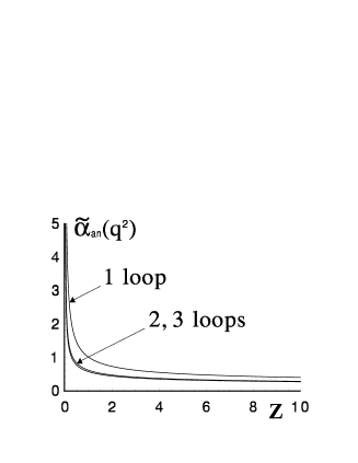
Figure 1: The QCD analytic invariant charge (8) at different loop levels, $z=q^{2}/\Lambda^{2}$.

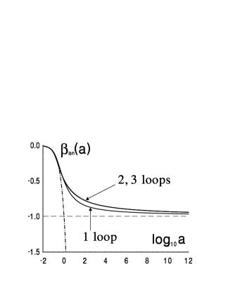
Figure 2: The $\beta$ function corresponding to the AIC (8) at different loop levels. The one-loop perturbative result is shown as the dot-dashed curve.

Figure 1 shows the running coupling $\widetilde{\alpha}_{\mbox{\scriptsize an}}(q^{2})=\alpha_{\mbox{\scriptsize an}}(q^{2})\,\beta_{0}/(4\pi)$ at different loop levels. In particular, it is follows from this figure that AIC (8) possesses a good higher loop stability. The study of the relevant $\beta$ function at the higher loop levels also enables one to elucidate the asymptotic behavior of the AIC. So, the $\beta$ function in hand

$$\beta^{(\ell)}_{\mbox{\scriptsize an}}(a)=\frac{d\,\ln a(\mu^{2})}{d\,\ln\mu^{2}},\qquad a(\mu^{2})\equiv\widetilde{\alpha}^{(\ell)}_{\mbox{\scriptsize an}}(\mu^{2})$$ (11)

was proved to have the universal asymptotics at any loop level [6]. Namely, it coincides with the perturbative result $\beta^{(1)}_{\mbox{\scriptsize s}}(a)=-a$ at small values of running coupling and tends to the minus unity at large $a$ (see Figure 2). In turn, this trait of the $\beta$ function implies that the AIC (8) itself possesses the universal asymptotics both in the ultraviolet $[\widetilde{\alpha}^{(\ell)}_{\mbox{\scriptsize an}}(q^{2})\simeq 1/\ln(q^{2}/\Lambda^{2})]$ and infrared $[\widetilde{\alpha}^{(\ell)}_{\mbox{\scriptsize an}}(q^{2})\simeq\Lambda^{2}/q^{2}]$ regions at any loop level. The detailed analysis of the properties of analytic running coupling can be found in Refs. [6, 7].

3 TIMELIKE REGION

For the consistent description of some strong interaction processes one has to employ the running coupling in the timelike region ($s=-q^{2}>0$). By making use of the prescription elaborated in Ref. [8] the continuation of AIC to the timelike domain has recently been performed

$$\widehat{\alpha}^{(\ell)}_{\mbox{\scriptsize an}}(s)=\frac{4\pi}{\beta_{0}}\,\int_{s/\Lambda^{2}}^{\infty}\rho^{(\ell)}(\sigma)\,\frac{d\sigma}{\sigma}$$ (12)

(see Ref. [5] for the details). Here the running coupling in the spacelike region is denoted by $\alpha(q^{2})$ and in the timelike region by $\widehat{\alpha}(s)$. It is worth noting also that the obtained result (12) confirms the hypothesis due to Schwinger concerning proportionality between the $\beta$ function and relevant spectral density (see Refs. [5, 8]).

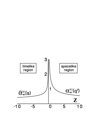
Figure 3: The one-loop analytic running coupling in the spacelike (7) and timelike (12) regions.

The plots of the one-loop analytic invariant charge in the spacelike and timelike domains are shown in Figure 3. In the ultraviolet limit these functions have identical behavior determined by the asymptotic freedom. However, there is asymmetry between them in the intermediate- and low-energy regions. The relative difference between $\widehat{\alpha}^{(1)}_{\mbox{\scriptsize an}}(s)$ and $\alpha^{(1)}_{\mbox{\scriptsize an}}(q^{2})$ is about several percents at the scale of the $Z$ boson mass, and increases when approaching the infrared domain. Apparently, this circumstance must be taken into account when one handles the experimental data.

4 PHENOMENOLOGICAL
APPLICATIONS

A decisive test of the self-consistency of any model for the strong interaction is its applicability to description of diverse QCD processes.

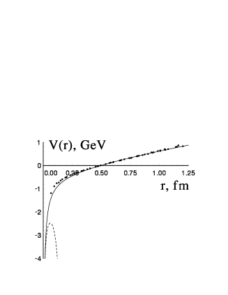
Figure 4: The constructed quark–antiquark potential $V(r)$ (solid curve) and the quenched lattice data ($\bullet$); $\Lambda=670\,$MeV, $n_{\mbox{\scriptsize f}}=0$. The dashed curve denotes the relevant perturbative result.

It was shown [4, 9] that the analytic running coupling (7) explicitly leads to the confining static quark–antiquark potential

$$V(r)\simeq\frac{8\pi}{3\beta_{0}}\frac{1}{r_{0}}\,\frac{r/r_{0}}{2\,\ln(r/r_{0})},\qquad r\to\infty,$$ (13)

where $r_{0}^{-1}=\Lambda\,e^{C}$ is a reference scale, and $C\simeq 0.577...$ denotes the Euler’s constant. At the same time, this potential has the standard behavior, determined by the asymptotic freedom, at small distances. The potential derived is found to be in a good agreement with the relevant lattice simulation data [10] (see Figure 4). The obtained one-loop estimation of the scale parameter $\Lambda=(670\pm 8)\,$MeV for $n_{\mbox{\scriptsize f}}=0$ active quarks corresponds to the value $\Lambda=(590\pm 10)\,$MeV in the region of three active quarks (see also Ref. [9]).

It was found [6] that there are symmetries, which relate the analytic invariant charge and the corresponding $\beta$ function in the UV and IR domains. One might anticipate that they could also be revealed in some intrinsically nonperturbative strong interaction processes. It is worth mentioning here the recently discovered symmetry related to the size distribution of instantons $D(\rho)$. Namely, the lattice simulation data [11] for the quantity $D^{\mbox{\tiny CI}}(\rho)=D(\rho)\left(\rho/\rho_{0}\right)^{N_{c}/6}$, where

$$D(\rho)=b\left[\frac{2\pi}{\alpha(\rho)}\right]^{2N_{c}}\exp\!\left[-\frac{2\pi}{\alpha(\rho)}\right],$$ (14)

have been observed to satisfy the conformal inversion symmetry $D^{\mbox{\tiny CI}}(\rho)=D^{\mbox{\tiny CI}}(\rho_{0}^{2}/\rho)$ [12]. In turn, this relation imposes a certain constraint onto the properties of the QCD running coupling $\alpha(\rho)$ at small and large distances. Proceeding from this, the analytic invariant charge (7) has recently been rediscovered and proved [12] to reproduce explicitly the conformal inversion symmetry of $D^{\mbox{\tiny CI}}(\rho)$.

The AIC has also been applied to description of the gluon condensate ($\Lambda=(631\pm 79)\,$MeV), inclusive $\tau$ lepton decay ($\Lambda=(524\pm 68)\,$MeV), and $e^{+}e^{-}$ annihilation into hadrons ($\Lambda=(490\pm 76)\,$MeV). Thus, the applications of the model developed to description of diverse strong interaction processes ultimately lead to congruous estimation of the parameter $\Lambda_{\mbox{\tiny QCD}}$. Namely, at the one-loop level with three active quarks $\Lambda=(557\pm 36)\,$MeV. Apparently, this testifies that the AIC substantially incorporates, in a consistent way, both perturbative and intrinsically nonperturbative aspects of Quantum Chromodynamics.

5 CONCLUSIONS

We have shown that the proposed way of involving the analyticity requirement into the RG method leads to qualitatively new features of the strong running coupling. Ultimately, this enables one to describe, in a consistent way, various strong interaction processes both of perturbative and intrinsically nonperturbative nature.

References

- [1] P.J. Redmond, Phys. Rev. 112 (1958) 1404; N.N. Bogoliubov, A.A. Logunov, and D.V. Shirkov, Sov. Phys. JETP 37 (1960) 574.
- [2] D.V. Shirkov and I.L. Solovtsov, Phys. Rev. Lett. 79 (1997) 1209.
- [3] I.L. Solovtsov and D.V. Shirkov, Theor. Math. Phys. 120 (1999) 482; D.V. Shirkov, Eur. Phys. J. C 22 (2001) 331.
- [4] A.V. Nesterenko, Phys. Rev. D 62 (2000) 094028.
- [5] A.V. Nesterenko, Phys. Rev. D 64 (2001) 116009.
- [6] A.V. Nesterenko and I.L. Solovtsov, Mod. Phys. Lett. A 16 (2001) 2517.
- [7] A.V. Nesterenko, Mod. Phys. Lett. A 15 (2000) 2401.
- [8] K.A. Milton and I.L. Solovtsov, Phys. Rev. D 55 (1997) 5295.
- [9] A.V. Nesterenko, hep-ph/0305091.
- [10] G.S. Bali et al., Phys. Rev. D 62 (2000) 054503.
- [11] D.A. Smith and M.J. Teper, Phys. Rev. D 58 (1998) 014505; A. Ringwald and F. Schrempp, Phys. Lett. B 459 (1999) 249; Phys. Lett. B 503 (2001) 331.
- [12] F. Schrempp, J. Phys. G 28 (2002) 915.