Next-to-leading order calculation of three-jet observables in hadron-hadron collision

Abstract

The production of the three jets in hadron-hardon collision is the first more complex process which allow us to define a branch of variables in order to do more precise measurement of the strong coupling and the parton distribution function of the proton. This process is also suitable for studying the geometrical properties of the hadronic final state at hadron colliders. This requires next-to-leading order prediction of the three-jet observables. In this paper we describe the theoretical formalism of such a calculation with sufficient details. We use a the dipole method to construct Monte Carlo program for calculating three-jet observables at next-to-leading order accuracy. We present a theoretical prediction for inclusive and exclusive cross section and for some relevant event shape variables like transverse thrust, transverse jet broadening and $E_{t3}$ variable.

I Introduction

In high energy hadron-hadron collision the processes with purely hadronic final state is one of the clearest processes to test the Quantum Chromodynamics (QCD) an measure its parameters simultaneously. According to the perturbative QCD the cross section of this processes is a convolution of a long- and a short distance part.

The long distance dependent part is the parton distribution function of the incoming hadrons. This function is universal, process independent and we can measure it in any basics process for example deeply inelastic scattering.

The short distance part is the partonic cross section that can be calculated in perturbative QCD as a function of a single parameter, the strong coupling (${\alpha_{s}}$). The main advantage of the hadronic final states at hadron-hadron colliders is that it is possible to measure the strong coupling and the PDF function simultaneously.

The production of three jets is the first process which can provide complex final state to define a branch of jet observables in order to be able to do more precise measurement of the strong coupling and give better determination of the parton distribution function. On the other hand this process allow us to do more advanced studies of the hadronic final states by measuring its geometrical properties. In order to be able to make quantitative prediction it is essential to perform the computations at least next-to-leading (NLO) accuracy. In hadron collision the most easily calculated one- and two-jet cross sections have so far been calculated at NLO level Giele et al. (1993); Kunszt and Soper (1992). At next-to-leading level some inclusive three-jet observables were calculated by Giele and Kilgore Kilgore and Giele ; Kilgore and Giele (1997) and by the author Nagy (2002). Furthermore, Z. Trócsányi also calculated the three-jet cross section in effective parton distribution function approximation Trócsányi (1996).

The main difficulty of the next-to-leading order calculations is the presence of the singularities. In general, when evaluating higher order QCD cross section, one has to consider real-emission contributions and virtual corrections and one has to deal with different type of the singularities. The ultraviolet singularities presented in the virtual contributions and they are removed by the renormalization. The infrared singularities presented both in the virtual and real contribution but the sum of them is finite. In the last few years the theoretical developments made possible the next-to-leading order calculation for three-jet quantities. There are several general methods available for the cancellation of the infrared divergences that can be used for setting up a Monte Carlo program Nagy and Trócsányi (1997); Frixione et al. (1996); Catani and Seymour (1997). In computing the NLO correction we use the dipole formalism of Catani-Seymour Catani and Seymour (1997) that we modified slightly in order to have a better control on the numerical calculation. This scheme is discussed in details in the next section.

The advantages of using the dipole method are the followings: i) no approximation is made; ii) the exact phase space factorization allows full control over the efficient generation of the phase space; iii) neither the use of color ordered subamplitudes, nor symmetrization, nor partial fractioning of the matrix elements is required; iv) Lorentz invariance is maintained, therefore, the switch between various frames can be achieved by simply transforming the momenta; v) the use of crossing functions is avoided; vi) it can be implemented in an actual program in a fully process independent way.

The important theoretical development that made possible the three-jet calculation was that the relevant one-loop amplitudes for the relevant subprocesses became available. For the $0\to ggggg$ Bern et al. (1993), $0\to q\bar{q}ggg$ subprocesses the amplitudes were calculated by Bern, Dixon and Kosower Bern et al. (1995) and for the $0\to q\bar{q}Q\bar{Q}g$ subprocess it was given by Kunszt, Signer and Trócsányi Kunszt et al. (1994). The relevant six parton tree-level matrix elements are also available Gunion and Kunszt (1985, 1986a, 1986b); Kuijf (1991).

In this paper we give sufficient details of our work and present several new results for next-to-leading order prediction of three-jet observables in hadron-hadron collision that were not published before and they could be interesting in an experimental analysis. In the Sec. II we give details of the analytic and numeric calculation and describe the structure of our result. In the Sec. III we present complete NLO predictions for three-jet inclusive cross sections and their energy fraction distribution (Dalitz variables) using the inclusive $k_{\perp}$-algorithm Ellis and Soper (1993) and the midcone algorithm Blazey et al. (2000). We define the thrust and jet broadening event shapes variables in the transverse plane. We show some subjet result using the exclusive $k_{\perp}$-algorithm Catani et al. (1993). Sec. IV contains our conclusion.

II Details of the calculation

II.1 The method

The next-to-leading order cross section for the process with two initial state hadrons is the convolution of the parton density functions of the incoming hadrons and the hard scattering cross section,

$$\sigma(p,\bar{p})=\sum_{a,b}\int_{0}^{1}\!\!d\eta\,f_{a/H}(\eta,\mu_{F}^{2})\int_{0}^{1}\!\!d\bar{\eta}\,f_{b/\bar{H}}(\bar{\eta},\mu_{F}^{2})$$

$$\times\left[\sigma^{LO}_{ab}(\eta p,\bar{\eta}\bar{p})+\sigma^{NLO}_{ab}(\eta p,\bar{\eta}\bar{p})\right]\;\;,$$ (1)

where $f_{i/H}$ is the density of the partons of type $i$ in the incoming hadron $H$ at the $\mu_{F}$ factorization scale. The corresponding parton level cross sections are

$$\sigma^{LO}_{ab}(p,\bar{p})\equiv\int_{3}d\sigma^{B}_{ab}(p,\bar{p})=\int_{3}d\Gamma^{(3)}\langle|{\cal M}^{(3)}_{ab}|^{2}\rangle F_{J}^{(3)}\;\;,$$ (2)

and the next-to-leading order correction is sum of three integrals

$$\sigma^{NLO}_{ab}(p,\bar{p})\equiv\int d\sigma^{NLO}_{ab}(p,\bar{p})$$

$$\quad=\int_{4}d\sigma^{R}_{ab}(p,\bar{p})+\int_{3}d\sigma^{V}_{ab}(p,\bar{p})+\int_{3}d\sigma^{C}_{ab}(p,\bar{p})\;\;,\qquad$$ (3)

where $d\sigma^{R}$ and $d\sigma^{V}$ are the real and virtual contributions to the cross section. The contribution $d\sigma^{C}$ represents the collinear subtraction counter term. The pole structure of this term is well defined but the finite part is factorization scale dependent. The actual form of the finite part in the expression of the $d\sigma^{C}$ defines the factorization scheme. In our calculations we chose the commonly used $\overline{\rm MS}$ subtraction scheme. The parton density functions are also scheme dependent, so that this dependence cancels in the hadronic cross section of Eq. (II.1).

The three integrals on the right hand side of Eq. (II.1) are separately divergent but their sum is finite provided by the jet function $F_{J}^{(m)}$ defines an infrared safe quantity, which formally means that

$$F_{J}^{(4)}\longrightarrow F_{J}^{(3)}\;\;,$$ (4)

in any case where the four-parton and three-parton configurations are kinematically degenerate. The presence of the singularities means that the separate pieces have to be regularized and the divergences have to be cancelled. We use the dimensional regularization in $d=4-2\epsilon$ dimensions in which case the divergences are replaced double poles $1/\epsilon^{2}$ and single poles $1/\epsilon$. We assume that ultraviolet renormalization of all Green functions to one-loop order has been carried out, so the divergences are infrared origin. In order to get the finite sum a slightly modified version of the Catani-Seymour Catani and Seymour (1997) dipole method is used in our calculations.

The reason for modifying the original dipole formalism is numerical. The essence of the dipole method is to define a single subtraction term $d\sigma^{A}$, the dipole subtraction term, that regularizes the divergences in the real term which comes form the soft and collinear regions. Thus, the three singular integrals in Eq. (II.1) are substituted by three finite ones:

$$\sigma^{NLO}_{ab}(p,\bar{p})=\sigma^{NLO}_{ab\{4\}}(p,\bar{p})+\sigma^{NLO}_{ab\{3\}}(p,\bar{p})$$

$$\quad+\int_{0}^{1}dx\left[\hat{\sigma}^{NLO}_{ab\{3\}}(x,xp,\bar{p})+\hat{\sigma}^{NLO}_{ab\{3\}}(x,p,x\bar{p})\right]\;\;,\qquad$$ (5)

where the four-parton integral is given by

$$\sigma^{NLO}_{ab\{3\}}(p,\bar{p})=\int_{4}\left[d\sigma^{R}_{ab}(p,\bar{p})_{\epsilon=0}-d\sigma^{A}_{ab}(p,\bar{p})_{\epsilon=0}\right]\;\;.$$ (6)

We have two three-parton contribution to the NLO correction. The second term on the right hand side of Eq. (II.1) is the sum of the one-loop contribution and a Born term convoluted by an universal singular factor $\mathrm{I}$,

$$\sigma^{NLO}_{ab\{3\}}(p,\bar{p})=\int_{3}\left[d\sigma^{V}_{ab}(p,\bar{p})+d\sigma^{B}_{ab}(p,\bar{p})\otimes{\mbox{\boldmath$\mathrm{I}$}}\right]_{\epsilon=0}\;\;.$$ (7)

The factor $\mathrm{I}$ contains all the $\epsilon$ poles which come from the $d\sigma^{A}$ and $d\sigma^{C}$ that are necessary to cancel the (equal and with opposite sign) poles in $d\sigma^{V}$. The last term in Eq. (II.1) is a finite remainder that is left after factorization of initial-state collinear singularities into the non-perturbative distribution functions (parton density function),

$$\int_{0}^{1}dx\,\hat{\sigma}^{NLO}_{ab\{3\}}(x,xp,\bar{p})=\sum_{a^{\prime}}\int_{0}^{1}dx$$

$$\qquad\int_{3}\left[d\sigma^{B}_{a^{\prime}b}(xp,\bar{p})\otimes({\mbox{\boldmath$\mathrm{P}$}}(x)+{\mbox{\boldmath$\mathrm{K}$}}(x))^{aa^{\prime}}\right]_{\epsilon=0}\;,$$ (8)

where the $x$-dependent functions $\mathrm{P}$ and $\mathrm{K}$ are similar (but finite for $\epsilon\to 0$) to the factor $\mathrm{I}$. These functions are universal, that is, they are independent of scattering process and of the jet observables.

There are several ways to define the $d\sigma^{A}$ dipole subtraction term, but all must lead to the same finite next-to-leading order correction. In this program a slight modification of the Catani-Seymour subtraction term was implemented by defining the dipole term as a function of a parameter $\alpha\in(0,1]$ which controls the volume of the dipole phase space. In the $e^{+}e^{-}$ annihilation case this modification of the dipole formalism was discussed in Ref. Nagy and Trocsanyi (1999) what we generalize for the hadron-hadron collision.

In this subsection we recall only those dipole factorization formulaes that are relevant in our calculation. We don’t want to give the precise definition of every variables, functions, factors we just use the same notation of the original paper of the dipole method Catani and Seymour (1997).

The $d\sigma^{A}$ local counter term is provided by the dipole factorization of the tree level squared matrix element. Thus we can define

$$d\sigma_{ab}^{A} = \sum_{\{4\}}d\Gamma^{(4)}(p_{a},p_{b},p_{1},...,p_{4})\frac{1}{S_{\{4\}}}$$ (9)

$$\qquad\times\Bigg{\{}\sum_{\mathrm{pairs}\atop i,j}\sum_{k\neq i,j}{\cal D}_{ij,k}(p_{a},p_{b},p_{1},...,p_{4})F_{J}^{(3)}(p_{a},p_{b},p_{1},..,\tilde{p}_{ij},\tilde{p}_{k},..,p_{4})\Theta(y_{ij,k}<\alpha)$$

$$\qquad\qquad+\sum_{\mathrm{pairs}\atop i,j}\left[{\cal D}_{ij}^{a}(p_{a},p_{b},p_{1},...,p_{4})F_{J}^{(3)}(\tilde{p}_{a},p_{b},p_{1},..,\tilde{p}_{ij},..,p_{4})\Theta(1-x_{ij,a}<\alpha)+(a\leftrightarrow b)\right]$$

$$\qquad\qquad+\sum_{i\neq k}\left[{\cal D}_{k}^{ai}(p_{a},p_{b},p_{1},...,p_{4})F_{J}^{(3)}(\tilde{p}_{a},p_{b},p_{1},..,\tilde{p}_{k},..,p_{4})\Theta(u_{i}<\alpha)+(a\leftrightarrow b)\right]$$

$$\qquad\qquad+\sum_{i}\left[{\cal D}^{ai,b}(p_{a},p_{b},p_{1},...,p_{4})F_{J}^{(3)}(\tilde{p}_{a},p_{b},\tilde{p}_{1},...,\tilde{p}_{4})\Theta(\tilde{v}_{i}<\alpha)+(a\leftrightarrow b)\right]\Bigg{\}}\;\;,$$

where $d\Gamma^{(4)}$ is the four-parton phase space including all the factors that are QCD independent, $\sum_{\{4\}}$ denotes the sum over all the configurations with $4$ partons and $S_{\{4\}}$ is the Bose symmetry factor of the identical partons in the final state. The ${\cal D}_{ij,k}$, ${\cal D}_{ij}^{a}$, ${\cal D}_{k}^{ai}$ and ${\cal D}^{ai,b}$ are the dipole terms. The function $F_{J}^{(3)}$ is the jet function which acts over the three-parton dipole phase space. The $y_{ij,k}$, $x_{ij,a}$, $u_{i}$, $\tilde{v}_{i}$ are the dipole variables defined by the dipole factorization of the phase space. The dipole factorization of the phase space is exact phase space factorization which means there is no approximation used in the kinematically degenerated regions (soft, collinear and soft-collinear). We found it makes the Monte Carlo integral more stable because the real contribution and the subtraction terms are defined in same phase space point.

In Eq. (9) the $\alpha=1$ case means the full dipole subtraction and it gives back the original dipole subtraction terms. In a computer program the large number of dipoles terms and complicated analytic structure of the expressions makes the evaluation of the subtraction terms rather time consuming. Using this cut dipole phase space we can speed up the program. The parameter $\alpha$ is also useful to check our program by varying the value of $\alpha$ and checking whether the full correction is independent of this parameter.

The most serious numerical defect of the subtraction schemes is the missed binning. This happens when a huge positive weight from the real part and the corresponding huge negative weight form the subtraction term are filled into different histogram bins. It is obvious this cut can increase the numerical stability of the Monte Carlo program by decreasing the size of the dipole phase space which reduces the chance of the missed binning.

The introduced $\alpha$ phase space cut parameter requires to redefine the $\mathrm{I}$ and ${\mbox{\boldmath$\mathrm{K}$}}(x)$ flavour kernels. The singular factor $\mathrm{I}$ is given by

$${\bf I}(p_{1},...,p_{m};\alpha;\epsilon) = -\frac{{\alpha_{s}}}{2\pi}\frac{1}{\Gamma(1-\epsilon)}\sum_{I}\frac{1}{{\mbox{\boldmath$\mathrm{T}$}}_{I}^{2}}{\cal V}_{I}(\alpha,\epsilon)$$ (10)

$$\times \sum_{J\neq I}{\mbox{\boldmath$\mathrm{T}$}}_{I}\cdot{\mbox{\boldmath$\mathrm{T}$}}_{J}\left(\frac{4\pi\mu^{2}}{2p_{I}p_{J}}\right)^{\epsilon}\;\;,\;\;$$

where the indices $I,J$ runs over both final and initial state parton and the $p_{I}\cdot p_{J}$ dot-products are always positive and

$${\cal V}_{i}(\alpha,\epsilon) = {\mbox{\boldmath$\mathrm{T}$}}_{i}^{2}\left(\frac{1}{\epsilon^{2}}-\frac{\pi^{2}}{3}\right)+\gamma_{i}\frac{1}{\epsilon}$$ (11)

$$+ \gamma_{i}+K_{i}(\alpha)+{\cal O}(\epsilon)\,,$$

where

$$K_{i}(\alpha)=K_{i}-{\mbox{\boldmath$\mathrm{T}$}}_{i}^{2}\ln^{2}\alpha+\gamma_{i}\left(\alpha-1-\ln\alpha\right)\;\;.$$ (12)

The $K_{i}$ and $\gamma_{i}$ constants are defined in the Eq. (5.90) and Eq. (7.28) in Ref. Catani and Seymour (1997). The ${\mbox{\boldmath$\mathrm{K}$}}(x,\alpha)$ flavour kernel is given by the followings:

$${\bf K}^{a,a^{\prime}}(x,\alpha) = \frac{{\alpha_{s}}}{2\pi}\Bigg{\{}\overline{K}^{aa^{\prime}}(x,\alpha)-K^{aa^{\prime}}_{F.S.}(x)-{\mbox{\boldmath$\mathrm{T}$}}_{b}\cdot{\mbox{\boldmath$\mathrm{T}$}}_{a^{\prime}}\frac{1}{{\mbox{\boldmath$\mathrm{T}$}}_{a^{\prime}}^{2}}\widetilde{K}^{aa^{\prime}}(x,\alpha)$$ (13)

$$\qquad+\delta^{aa^{\prime}}\sum_{i}{\mbox{\boldmath$\mathrm{T}$}}_{i}\cdot{\mbox{\boldmath$\mathrm{T}$}}_{a}\frac{\gamma_{i}}{{\mbox{\boldmath$\mathrm{T}$}}_{i}^{2}}\left[\left(\frac{1}{1-x}\right)_{1-\alpha}+\alpha\,\delta(1-x)\right]\Bigg{\}}\;\;,\qquad\quad$$

where $K^{aa^{\prime}}_{F.S.}(x)$ is defined by the factorization scheme. In the case of the $\overline{\mathrm{MS}}$ scheme this functions are identically zero. The flavour functions $\overline{K}^{ab}(x,\alpha)$ are

$$\overline{K}^{ab}(x,\alpha) = \hat{P}^{\prime}_{ab}(x)+P^{ab}_{reg}(x)\ln\frac{\alpha(1-x)}{x}+\delta^{ab}{\mbox{\boldmath$\mathrm{T}$}}_{a}^{2}\delta(1-x)\ln^{2}\alpha$$ (14)

$$+ \delta^{ab}\left[{\mbox{\boldmath$\mathrm{T}$}}_{a}^{2}\left(\frac{2}{1-x}\ln\frac{1-x}{x}\right)_{+}-\delta(1-x)\left(\gamma_{a}+K_{a}(\alpha)-\frac{5}{6}\pi^{2}{\mbox{\boldmath$\mathrm{T}$}}_{a}^{2}\right)\right]$$

$$+ \delta^{ab}{\mbox{\boldmath$\mathrm{T}$}}_{a}^{2}\frac{2}{1-x}\left(\ln\frac{\alpha(2-x)}{1+\alpha-x}-\ln\frac{2-x}{1-x}\Theta(x<1-\alpha)\right)\;\;.$$

The $\widetilde{K}^{ab}(x,\alpha)$ flavour kernels are defined by

$$\widetilde{K}^{ab}(x,\alpha) = P_{reg}^{ab}(x)\ln\frac{1-x}{\alpha}+<\hat{P}_{a,b}(x,\epsilon=0)>\ln\alpha(x)-\delta^{ab}{\mbox{\boldmath$\mathrm{T}$}}_{a}^{2}\left[\left(\frac{2}{1-x}\ln\frac{1}{1-x}\right)_{1-\alpha}+\frac{\pi^{2}}{3}\delta(1-x)\right]$$ (15)

$$+ \delta^{ab}{\mbox{\boldmath$\mathrm{T}$}}_{a}^{2}\frac{2}{1-x}\left[\ln\frac{1+\alpha-x}{\alpha}-\ln(2-x)\Theta(x>1-\alpha)\right]\;\;,$$

where function $\alpha(x)$ is given by the following

$$\alpha(x)=\min\left\{1,\frac{\alpha}{1-x}\right\}\;\;.$$ (16)

The definition of the Altarelli-Parisi probabilities ($P^{ab}_{reg}(x)$, $\hat{P}^{\prime}_{ab}(x)$) and splitting functions ($<\hat{P}_{a,b}(x,\epsilon)>$) are given in Appendix C in Ref. Catani and Seymour (1997). The “$\beta=1-\alpha$” prescription is defined by

$$\int_{0}^{1}dx\left(\frac{1}{1-x}\right)_{\beta}f(x)=\int_{\beta}^{1}dx\frac{f(x)-f(1)}{1-x}\;\;.$$ (17)

II.2 Structure of the results

Once the phase space integrations are carried out, we write the NLO jet cross section in the following form:

$$\sigma^{n\rm{jet}}_{AB} = \sum_{a,b}\int_{0}^{1}d\eta\int_{0}^{1}d\bar{\eta}f_{a/A}(\eta,\mu_{F}^{2})f_{b/B}(\bar{\eta},\mu_{F}^{2})$$ (18)

$$\times \hat{\sigma}_{ab}^{n\rm{jet}}\left[p_{a},p_{b},{\alpha_{s}}(\mu_{R}^{2}),\mu_{R}^{2}/Q_{HS}^{2},\mu_{F}^{2}/Q_{HS}^{2}\right]\;,\;$$

where $f_{i/H}(\eta,\mu_{F}^{2})$ represents the patron distribution function of the incoming hadron defined at the factorization scale $\mu_{F}=x_{F}Q_{HS}$, $\eta_{a,b}$ is the fraction of the proton momentum carried by the scattered partons $p_{a,b}$, $Q_{HS}$ is the hard scale that characterizes the parton scattering which could be $E_{T}$ of the jet, jet mass of the event, etc and $\mu_{R}=x_{R}Q_{HS}$ is the renormalization scale.

In the presented leading- and next-to-leading order results we use the C/C++ implementation c-l of the LHAPDF library Giele et al. (2001) with CTEQ6 Pumplin et al. (2002) parton distribution function and with the corresponding ${\alpha_{s}}$ expression which is included in this library. The CTEQ6 set was fitted using the two-loop running coupling with ${\alpha_{s}}(M_{Z^{0}})=0.118$.

To ensure the correctness of the result several check was performed: (i) the Born level two-, three- and for-jet cross sections were compared to the prediction of NJETS Kuijf (1991) program and perfect agreement was found; (ii) singular behaviour of the real and dipole subtraction terms were checked numerically in randomly chosen phase space points; (iii) the total NLO corrections was independent of the $\alpha$ parameters that controls the dipole phase space; (iv) the program is based on the NLOJET++ program library c-l that was used other already well tested processes.

In the NLO calculation the difference of the real contributions and the dipole subtraction terms is still singular but these are integrable square root singularities. Integrating these singularities by simple Monte Carlo integration technique (choosing random values of the integration variables uniformly) is not efficient way because the variance of the estimate of the integral is infinite and we are not able to estimate the statistical error of the integral. To improve the stability and the convergence of the Monte Carlo integral the phase space is generated by multi-channel weighted phase space generator Kleiss and Pittau (1994).

III Results

In this section we study those jet observables which could be interesting in the jet studies at hadron-hadron colliders. We show some examples of inclusive three-jet cross sections, energy fraction distributions of the jets, event shapes variables and sub-jet rates. To present inclusive jet cross section and some related jet observables like energy fraction distribution we use the Ellis-Soper inclusive $k_{\perp}$ algorithm Ellis and Soper (1993) and the midpoint cone algorithm Blazey et al. (2000). To do sub-jet studies and calculate some jet clustering algorithm related event shape variable like flipping variable we use the exclusive $k_{\perp}$ algorithm which was defined by Catani et. al. in Ref. Catani et al. (1993). We also present some jet clustering independent event shape distribution which are defined in the transverse plane (transverse thrust and transverse jet broadening).

III.1 Three-jet inclusive cross sections

The most important jet quantities are the inclusive jet cross section and its transverse distribution. In hadron-hadron collision for jet studies a variant of the cone algorithms was used. Unfortunately those algorithms which were used at the first run of the Tevatron are infrared and/or collinear unsafe or only safe up to a given order in the perturbative calculation. It is essential that the used jet algorithm to be infrared safe all order otherwise the perturbative calculation and the perturbative prediction are unstable. Using an almost infrared unsafe jet algorithm we are not able to estimate the effect of the higher order contributions due to the variation of the renormalization and factorization scales. The other problem with this type of the jet algorithms is that they are logarithmically sensitive to the detector resolution (energy and angular resolution). That is bad because in the fix order perturbative calculation it is impossible or hard to consider or simulate precisely these effects Seymour (1998).

In this subsection we use the Ellis-Soper inclusive $k_{\perp}$ algorithm and the midcone iterative cone algorithm which are infrared and collinear safe to all orders. In both cases we consider only those jets as hard final state jets which have at least $20$GeV transverse energy and are in the $|\eta|<2$ pseudo-rapidity interval. The total jet transverse energy must be larger than $80$GeV. The renormalization and factorization scales are characterised by the hard scale which is the third of the total jet transverse momentum

$$Q_{HS}=\frac{1}{3}\sum_{j=1}^{n_{J}}p_{T}^{\mathrm{jet}}(j)\;\;.$$ (19)

All jet contributes to this sum which passed the cuts.

Figure 1: The fix order QCD predictions for the inclusive three-jet differential cross sections of the transverse momentum of the leading jet obtained using the inclusive $k_{\perp}$ and midcone algorithms. The bands indicate the theoretical uncertainty due to the variation of the scales $x_{R,F}$ between $0.5$ and $2$. The grey band is the leading order and the dark grey band is the next-to-leading order. The inset figures show the $K$ factor and its scale dependence. The solid line represents the $x_{R,F}=1$ scale choice.

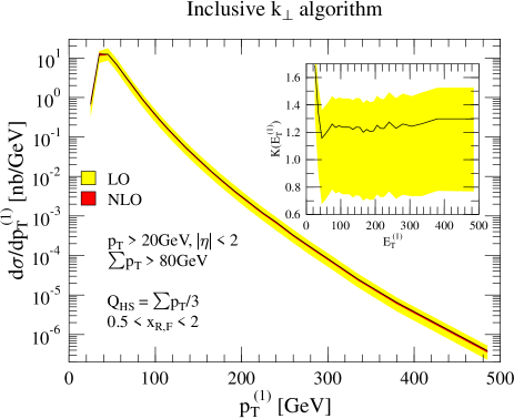
Calculating the transverse energy distribution of the leading jet and comparing the leading and the next-to-leading order fix order predictions we can see in the $k_{\perp}$ case if the scales are set to $x_{R,F}=1$ the NLO correction is about $25-30\%$ as shown in Figure 1. The $K=\sigma^{NLO}/\sigma^{LO}$ factor strongly depends on the scale choice but the NLO prediction is stable. Varying the scales between $0.5$ and $2$ the scale uncertainty of the NLO prediction is about $8-10\%$ which is significantly smaller than the leading order uncertainty which is about $100\%$ or more.

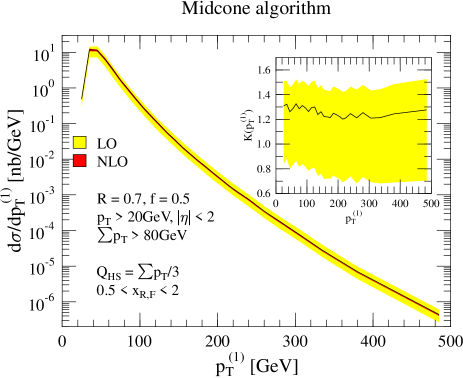
Using the midcone algorithm we got a very similar result. In this calculation the cone size is $R=0.7$ and the merge/split threshold parameter is $f=0.5$. In this case the NLO correction is about $20-30\%$ with the $x_{R,F}=1$ scales.

In Table 1 the NLO cross sections are tabulated. Comparing the values we can see that $k_{\perp}$ algorithm gives higher cross section in the low $E_{T}$ region while in the high $E_{T}$ region the cone result is higher. The difference between the two results is less than $10\%$ almost everywhere.

Table 1: Next-to-leading order results for the differential distribution the three jet inclusive cross sections as function of the transverse energy of leading jet. The scales are $x_{R,F}=1$. The errors are the statistical error of the Monte Carlo integration.

$E_{T}^{(1)}$	$k_{\perp}$ algorithm	midcone algorithm
GeV	nb/GeV	nb/GeV
$20-30$	$(6.745\pm 0.240)\cdot 10^{-1}$	$(4.961\pm 0.387)\cdot 10^{-1}$
$30-40$	$(1.245\pm 0.009)\cdot 10^{1}$	$(1.174\pm 0.019)\cdot 10^{1}$
$40-50$	$(1.252\pm 0.009)\cdot 10^{1}$	$(1.148\pm 0.014)\cdot 10^{1}$
$50-60$	$(6.966\pm 0.042)\cdot 10^{0}$	$(6.522\pm 0.077)\cdot 10^{0}$
$60-70$	$(3.509\pm 0.020)\cdot 10^{0}$	$(3.338\pm 0.034)\cdot 10^{0}$
$70-80$	$(1.799\pm 0.009)\cdot 10^{0}$	$(1.662\pm 0.017)\cdot 10^{0}$
$80-90$	$(9.175\pm 0.049)\cdot 10^{-1}$	$(9.003\pm 0.096)\cdot 10^{-1}$
$90-100$	$(4.991\pm 0.026)\cdot 10^{-1}$	$(4.884\pm 0.054)\cdot 10^{-1}$
$100-110$	$(2.755\pm 0.015)\cdot 10^{-1}$	$(2.713\pm 0.028)\cdot 10^{-1}$
$110-120$	$(1.583\pm 0.009)\cdot 10^{-1}$	$(1.595\pm 0.018)\cdot 10^{-1}$
$120-130$	$(9.362\pm 0.057)\cdot 10^{-2}$	$(9.452\pm 0.011)\cdot 10^{-2}$
$130-140$	$(5.554\pm 0.035)\cdot 10^{-2}$	$(5.607\pm 0.069)\cdot 10^{-2}$
$140-150$	$(3.461\pm 0.022)\cdot 10^{-2}$	$(3.517\pm 0.045)\cdot 10^{-2}$
$150-160$	$(2.164\pm 0.015)\cdot 10^{-2}$	$(2.152\pm 0.030)\cdot 10^{-2}$
$160-170$	$(1.350\pm 0.010)\cdot 10^{-2}$	$(1.398\pm 0.019)\cdot 10^{-2}$
$170-180$	$(8.784\pm 0.068)\cdot 10^{-3}$	$(9.103\pm 0.135)\cdot 10^{-3}$
$180-190$	$(5.725\pm 0.049)\cdot 10^{-3}$	$(6.110\pm 0.099)\cdot 10^{-3}$
$190-200$	$(3.806\pm 0.032)\cdot 10^{-3}$	$(4.014\pm 0.065)\cdot 10^{-3}$
$200-210$	$(2.592\pm 0.022)\cdot 10^{-3}$	$(2.698\pm 0.048)\cdot 10^{-3}$
$210-220$	$(1.740\pm 0.016)\cdot 10^{-3}$	$(1.786\pm 0.034)\cdot 10^{-3}$
$220-230$	$(1.185\pm 0.011)\cdot 10^{-3}$	$(1.243\pm 0.025)\cdot 10^{-3}$
$230-250$	$(7.048\pm 0.057)\cdot 10^{-4}$	$(7.503\pm 0.121)\cdot 10^{-4}$
$250-270$	$(3.270\pm 0.036)\cdot 10^{-4}$	$(3.471\pm 0.080)\cdot 10^{-4}$
$270-290$	$(1.646\pm 0.020)\cdot 10^{-4}$	$(1.797\pm 0.042)\cdot 10^{-4}$
$290-320$	$(7.041\pm 0.068)\cdot 10^{-5}$	$(7.754\pm 0.155)\cdot 10^{-5}$
$320-350$	$(2.530\pm 0.031)\cdot 10^{-5}$	$(2.781\pm 0.057)\cdot 10^{-5}$
$350-410$	$(6.471\pm 0.064)\cdot 10^{-6}$	$(6.993\pm 0.129)\cdot 10^{-6}$
$410-560$	$(3.864\pm 0.044)\cdot 10^{-7}$	$(4.391\pm 0.096)\cdot 10^{-7}$

III.2 Topology of the three-jet events

One can study the structure of the three-jet events. We can define variables which test certain properties of the jets. These quantities could be any azimuthal correlation between the jets or the energy fraction of the three leading jets.

The energy fraction of the three leading jets (leading in transverse energy) was measured by the CDF collaboration Abe et al. (1992); Brandl and Seidel (2000). This quantity is defined in centre of mass frame of the three jets. The jets are ordered and labeled by energy in the rest frame ($E_{1}\,>\,E_{2}\,>\,E_{3}$). The energy fraction variable (usually called Dalitz variables) are given by

$$X_{i}=\frac{2E_{i}}{E_{1}+E_{2}+E_{3}}\;\;,\qquad i=1,2,3\;\;.$$ (20)

The variable $X_{1}$ varies between $2/3$ and $1$, $X_{2}$ between $1/2$ and $1$, and $X_{3}$ between $0$ and $2/3$. There are only two independent variables since $X_{1}+X_{2}+X_{3}=2$. We use only the first two variables.

In the experimental analysis the iterative cone algorithm was used with an additional cut on the jets. It was required that the jets were well separated. This additional cut ensures that the cross section is calculable order by order in perturbation theory but the jet algorithm is still not fully infrared safe, it is almost infrared unsafe Seymour (1998).

To get stable theoretical predictions in our calculations we use the inclusive $k_{\perp}$ and midcone jet algorithms to resolve jets with the same cuts what was used in Ref. Brandl and Seidel (2000). All jets are required to have at least $20$GeV transverse energy and they must lay in the $|\eta|<2$ pseudo-rapidity window. We calculate the normalised differential distributions of the $X_{1}$ and $X_{2}$ variables and the double differential distribution of these variables. In these calculations the renormalization and factorization scales are set to the third of the total jet transverse energy Eq. (19).

Figure 2: The scale dependence of the total 3-jet cross sections.

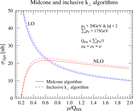
The distributions are normalised by the total 3-jet cross section plotted in Figure 2. We can see the NLO correction reduced the scale dependence of perturbative prediction. The scale uncertainty of the NLO result is about $10-12\%$ varying the scales on the $0.6<x_{R,F}<2$ range while the LO uncertainty is much higher $38-40\%$. The corrections with the $x_{R,F}=1$ scale choice are about $30\%$.

Figure 3: Next-to-leading order perturbative prediction for normalised double differential distribution ($1/\sigma d\sigma/dX_{1}dX_{2}$) of the energy fraction variables $X_{1}$ and $X_{2}$ using the midcone and inclusive $k_{\perp}$ algorithm.

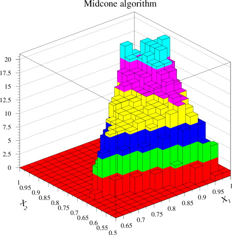
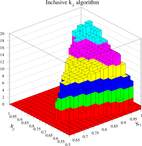
The double differential distributions of the variables $X_{1}$ and $X_{2}$ are plotted in Figures 3. The phase space would populate the available $X_{1}$, $X_{2}$ region uniformly. Deviation from the uniform distribution shows the effect of the QCD dynamics.

Taking the double differential distribution and projecting on either axis the distributions of variables $X_{1}$ and $X_{2}$ can be obtained.

Figure 4: The energy fraction distribution of the leading ($X_{1}$) and second leading ($X_{2}$) jets. The upper figure is result with the inclusive $k_{\perp}$ algorithm and the lower figures shows the midcone result.

In Figure 4 the differential distributions of the energy fractions are plotted in the inclusive $k_{\perp}$ and midcone algorithm cases.

Comparing the leading order result to the next-to-leading order result we can see that the NLO distribution of the leading jet is less peaked than the LO but in the case of the $X_{2}$ distribution the NLO result is more peaked around $0.65$. The NLO correction of the distributions is small.

Comparing the two algorithms to each other we can say that the distributions are very similar and there is not too much difference. The $X_{1}$ distribution of the inclusive $k_{\perp}$ algorithm is a little bit more peaked and the $X_{2}$ distribution is a little bit flatter than in the midcone case. The corresponding peaks are in the same positions.

III.3 Three-jet event shapes

We can distinguish two type of the event shapes. One can calculate and measure the event shapes which are associated to a jet algorithm. Generally we can say that this type of variables gives information about any geometrical property of the jets in a $n$-jet event. Or we can define event shape variables which measure any geometrical property of the event e.g thrust or jet bordering.

Using the exclusive $k_{\perp}$ algorithm there is a natural way to introduce event shape variables. The prescription of this algorithm introduces a stopping parameter $d_{cut}$ (resolution variable), that defines the hard scale of the process and separates the event into a hard scattering part and a low-$p_{T}$ part (beam-jet).

Defining the $d_{cut}$ resolution variable event-by-event we can calculate the differential distribution of the $E_{tn}$ event shape variable. Denoting by $d_{m}$ the smallest resolution variable when the event has $m$ hard final state jets the $E_{tn}$ event shape variable is defined by

$$E_{tn}^{2}=\max_{m\geq n}\{d_{m}\}\;\;.$$ (21)

Figure 5: Distribution of the $E_{t3}$ event shape variable at LO an NLO level. The bands indicate the theoretical uncertainty due to the variation of the scales $x_{R,F}$ between $0.5$ and $2$. The grey band is the leading order and the black band is the next-to-leading order. The inset figure shows the $K$ factor and its scale dependence. The solid line represents the $x_{R,F}=1$ scale choice.

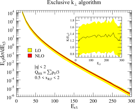
We plotted the differential distribution of the $E_{t3}$ event shape variable in Figure 5. In this calculation the $|\eta|<2$ pseudo-rapidity cut was applied for every hard final state jet. The renormalization and factorization scales were given by $\mu_{R,F}=x_{R,F}Q_{HS}$ where the hard scale is the average transverse momentum of the three jets

$$Q_{HS}=\frac{1}{3}\sum_{j=1}^{3}p_{T}^{\mathrm{jet}}(j)\;\;.$$ (22)

Comparing the next-to-leading order result to the leading order result we see that the LO prediction strongly depends on the scales. Varying the scale parameters $x_{R,F}$ between $0.5$ and $2$ the scale uncertainty of the NLO result is about $15\%$ in contrast to the LO scale uncertainty which is about $80\%$. Setting the scales to $x_{R,F}=1$ we see that the NLO correction is about $20-35\%$.

One can define event shapes on the transverse plane. Important example is the transverse thrust which is defined by

$$T_{\perp}=\max_{\vec{n}}\frac{\sum_{i\in C_{N}}|\vec{p}_{\perp,i}\cdot\vec{n}|}{\sum_{i\in C_{N}}|\vec{p}_{\perp,i}|}\;\;,$$ (23)

where $\vec{p}_{\perp,i}$ is the transverse component of the parton (hadron) momentum. The unit vector that $\vec{n}$ maximises the ratios of the sums is usually called thrust axis. In these sum only those particles are counted which are fulfil all selection criteria $C_{N}$. This selection must be infrared safe. In this calculation we required that the pseudo-rapidity of those particles which contribute to $T_{\perp}$ must be in the $[-1.1,1.1]$ pseudo-rapidity window thus we have

$$C_{N}=\{i\;\;:\quad|\eta_{i}|<1.1\;\;,\quad i=1,\dots,N\}\;\;,$$ (24)

where $N$ is the number of particles in the event. This definition of the thrust for hadron colliders gives an infrared safe longitudinally boost invariant quantity.

The jet broadening $B_{\perp}$ is an associated quantity to the thrust. Using the thrust axis we can define $B_{\perp}$ on the transverse plane by the following formulae

$$B_{\perp}=\frac{\sum_{i\in C_{N}}|\vec{p}_{\perp,i}\times\vec{n}|}{2\sum_{i\in C_{N}}|\vec{p}_{\perp,i}|}\;\;.$$ (25)

In Figure 6 the differential distributions of the transverse thrust and the transverse jet broadening have been plotted at LO and NLO level. In this calculation the total transverse energy is larger than $100$GeV

$$H_{T}\equiv\sum_{i\in C_{N}}E_{T,i}>100\mathrm{GeV}\;\;.$$ (26)

The perturbative results logarithmically divergent at the edge of the phase space. This divergence occurs at $T_{\perp}=1$ and $T=2/3$ in the thrust distribution and at $B_{\perp}=0$ and $B=1/3$ in the jet broadening distribution. Setting the scale to the total transverse energy the NLO order correction in the middle of the distribution where the effect of the logarithm is small is $30-35\%$ for the thrust and $20-45\%$ for jet broadening as it is shown in the inset figure. It is necessary to do all order resummation of the leading and next-to-leading logarithms to be able to do quantitative comparison of the theory to the data.

Figure 6: Distribution of $1-T_{\perp}$ and $B_{\perp}$ event shape variable at LO (dashed line) and NLO (solid line) level. The scales were set to $\mu_{R,F}=H_{T}$. The inset figure shows the $K$-factors.

One can define the average value of the event shape variables as function of the total transverse energy. This quantity is given bay the following ratio:

$$\langle O_{3}\rangle_{\delta}=\left(\frac{d\sigma}{dH_{T}}\right)^{-1}\int_{\delta}^{1}dO_{3}O_{3}\frac{d\sigma}{dO_{3}dH_{T}}\;\;,$$ (27)

where $O_{3}$ could be either $1-T_{\perp}$ or $B_{\perp}$.

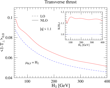
Figure 7 shows the average value of the transverse thrust. With the $\mu_{R,F}=H_{T}$ scale choice it was found that the NLO correction is small about $15\%$. The NLO correction doesn’t change the shape of the distribution as it is shown by the K-factor plot. This result indicate that the NLO fix order prediction might describe the data itself with good accuracy.

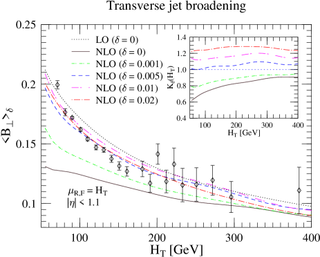
Figure 8 shows the average value of the transverse jet broadening. The CDF collaboration Abe et al. (1991) measured this distribution with $\delta=0$ choice and the data was compared to the leading order QCD prediction. Comparing the data to the NLO prediction the difference between the data and the theory is huge. This can happen because the contribution of the large logarithms from the small $B_{\perp}$ region is very large and in the NLO case it causes a huge negative effect. It is clear that the fix order calculation is unable to describe the data itself. The resummation of the large logarithms is important Banfi et al. (2003).

As shown in Fig. 6 the large negative contributions come form the small $B_{\perp}$ region ($B_{\perp}<0.02$). Resuming the leading and the next-to-leading logarithms the $B_{\perp}d\sigma/dB_{\perp}$ distribution is positive definite and we can expect that it is reasonable small in the small $B_{\perp}$ region. On the other hand Fig. 6 indicates that the NLO fix order calculation is stable prediction in the large ($B_{\perp}>0.2$) region. Assuming that the all order contribution of the $B_{\perp}<0.02$ region to the average value is small and changing the $\delta$ parameter we can make a better comparison of the data and the NLO prediction. In Fig. 8 we can see that the $\langle B_{\perp}\rangle_{0.0}$ and the $\langle B_{\perp}\rangle_{0.001}$ NLO results suffer on the effect of the large logarithm but changing the $\delta$ parameter between $0.005$ and $0.02$ the NLO prediction is stable and hardly depends on the $\delta$ parameter and the agreement with the data is much better. The inset figure shows the $K_{\delta}=\langle B_{\perp}\rangle_{\delta}^{NLO}/\langle B_{\perp}\rangle_{\delta}^{LO}$ factor. For $0.005<\delta<0.02$ the NLO correction is positive, nearly constant and it is maximum $30\%$.

Of course this is not a precise analysis and without the resummation of the leading and next-to-leading logarithms the quantitative comparison of the current data and the theory is impossible but it can help to understand the huge discrepancy between the data and the NLO prediction. It also indicate that the NLO prediction can describe the data itself very well if $\delta>0.005$.

Figure 7: Average value of the $1-T_{\perp}$ event shape variable at $\delta=0$ at LO (dashed line) and NLO (solid line) level. The scales were set to $\mu_{R,F}=H_{T}$. The inset figure shows the $K$-factor.

Figure 8: Average value of the $B_{\perp}$ event shape variable at $\delta=0$ at LO and NLO level for $\delta=0,0.001,0.005,0.01,0.02$. The scales were set to $\mu_{R,F}=H_{T}$. The markers (diamonds) and the error bars represent the CDF data Abe et al. (1991) and its statistical error. The inset figure shows the $K$-factors.

III.4 Sub-jet fractions

In this subsection we study the sub-jet multiplicities of the events. We use the exclusive $k_{\perp}$ algorithm Catani et al. (1993). The jets are defined in a two-step clustering procedure. The first step of the algorithm identifies the low-$p_{T}$ scattering fragments and includes them in the beam jets, thus factorizing the hard scattering subprocess. The scale of the hard final state jets is $E_{cut}$ the stopping parameter of this clustering step. Defining the sub-jet resolution variable $y_{cut}=Q_{0}/E_{cut}$ the second step of the algorithm resolves the sub-jet structure of the hard final state jets.

The $n$ sub-jet rate is defined by the ratio of the $n$ sub-jet cross section and the total cross section as

$$R_{n}(E_{cut},y_{cut})=\frac{\sigma_{n}(E_{cut},y_{cut})}{\sigma_{tot}(E_{cut})}\;\;,$$ (28)

where the $\sigma$ is the total cross section defined by the sum of the $n$-jet cross section at the $E_{cut}$ scale

$$\sigma_{tot}(E_{cut})=\sum_{n=2}^{\infty}\sigma_{n}(E_{cut})=\int_{E_{cut}}^{\infty}dE_{t2}\frac{d\sigma}{dE_{t2}}\;\;.$$ (29)

The $E_{t2}$ variable is the smallest value of the $E_{cut}$ resolution variable where the event has two jets. Using the similar event shape variables $y_{n}$ and $y_{n+1}$ of the second step we can define the exclusive sub-jet cross section at a given $E_{cut}$ scale by

$$\sigma_{n}(E_{cut},y_{cut}) = \int_{E_{cut}}^{\infty}dE_{t2}\left[\int_{y_{cut}}^{\infty}dy_{n}\frac{d\sigma}{dE_{t2}dy_{n}}\right.$$ (30)

$$\quad-\left.\int_{y_{cut}}^{\infty}dy_{n+1}\frac{d\sigma}{dE_{t2}dy_{n+1}}\right]\;\;.\;\;$$

In the fix order perturbation calculation we can calculate the $3$-sub-jet ratio at NLO level ($R_{3}^{NLO}(E_{cut},y_{cut})$) and the $4$-sub-jet ratio at LO level ($R_{4}^{LO}(E_{cut},y_{cut})$). From the definition of the $n$-sub-jet ratios we have the normalisation condition

$$1=\sum_{i=2}^{\infty}R_{n}(E_{cut},y_{cut})\;\;.$$ (31)

Using this relation the 2-sub-jet ration can be obtained at next-to-next-to-leading order level (NNLO)

$$R_{2}^{NNLO}(E_{cut},y_{cut})=1-R_{3}^{NLO}(E_{cut},y_{cut})$$

$$\qquad\qquad-R_{4}^{LO}(E_{cut},y_{cut})+{\cal O}({\alpha_{s}}^{3})\;\;.\;\;$$ (32)

Analogously to the $e^{+}e^{-}$-annihilation we can define the sub-jet multiplicity

$$N(E_{cut},y_{cut})=\sum_{n=2}^{\infty}nR_{n}(E_{cut},y_{cut})\;\;,$$ (33)

and at up to second order

$$N(E_{cut},y_{cut})=2+R_{3}^{NLO}(E_{cut},y_{cut})$$

$$\qquad\qquad+2R_{4}^{LO}(E_{cut},y_{cut})+{\cal O}({\alpha_{s}}^{3})\;\;.$$ (34)

The fix order perturbative predictions depend on the unphysical renormalization and factorization scales. In these calculations the scales are given by event-by-event basis. We use the invariant mass of the two hard final state jets found at $E_{t2}$ scale as renormalization and factorization scale

$$\mu^{2}_{R,F}=(p_{1}+p_{2})^{2}\;\;.$$ (35)

Figure 9: The fix order QCD prediction for the two-, three- and four-jet sub-jet rates and for the sub-jet multiplicity. The two-jet rate is calculated at NNLO, the three-jet rate is calculated at NLO and the four-jet at LO level.

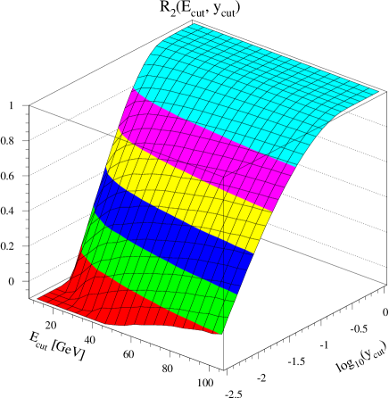
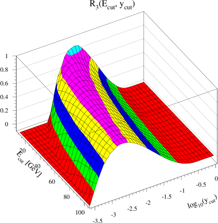
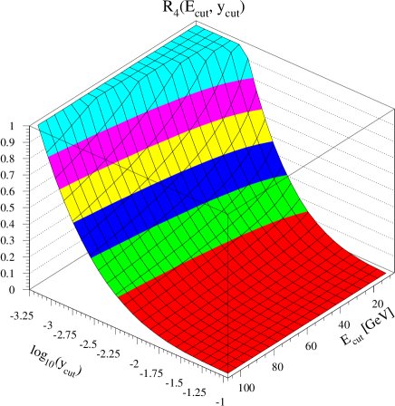
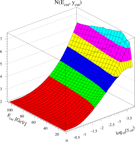
Fig.9 shows the sub-jet ratios and the sub-jet multiplicity. The result is given as function of $E_{cut}$ parameter and the logarithm based ten of the sub-jet resolution variable. The distributions are plotted on the $10<E_{cut}<110\ \mathrm{GeV}$ and $-3.9<\log_{10}(y_{cut})<0$ region. We can see the sub-jet ratios are strongly dominated by the large logarithms in the low $E_{cut}$ and $y_{cut}$ regions. To be able to do any quantitative comparison to the experimental data in this region it is necessary to sum at least the leading- and next-to-leading logarithms at all order and match it to the fix order calculation.

IV Conclusion

This paper dealt with the next-to-leading order calculation of three-jet observables in hadron-hadron collision. We gave a modification of the original dipole method that made possible to construct a Monte Carlo program for this process. We find this modified dipole subtraction method was very useful from the point of the numerical calculation. The introduced phase space cut in the dipole term could reduce the evaluation time of subtraction terms and increase the numerical stability of the Monte Carlo integral by reducing the probability of the missed binning.

We calculated the transverse momentum distribution of the leading jet of the three-jet inclusive cross section using the inclusive $k_{\perp}$ an midcone algorithms. We found that the NLO correction can stabilize the theoretical prediction by reducing the renormalization and factorization scale dependences significantly. We also calculated the energy fraction distribution of the three-jet inclusive cross section. Comparing the leading order result to the next-to-leading order result we found that the NLO corrections are negligible in these analysises.

We defined event shape variables in the transverse plane. We calculated the differential distribution of the transverse thrust and transverse jet broadening and the transverse energy dependence of the average values. We found that the size of the NLO correction is not too large and acceptable but at the edge of the available phase space the result suffers on the contribution of large logarithm. In this region a next-to-leading logarithmic approximation (NLL) matched with the fix order prediction can give reasonable result. The average value of the transverse jet broadening was compared to the CDF data and we found that the comparison of the current data and the theory without NLL resummation is impossible. Using a rough approximation in the small $B_{\perp}$ region we were able to do some qualitative comparison between data and the NLO QCD prediction and we found reasonable good agreement.

We also calculated the subjet rates and the subjet multiplicity using the exclusive $k_{\perp}$ algorithm. These quantities were defined in that way to mimic $e^{+}e^{-}$ annihilation like situation at hadron colliders. The result is very similar to what we have in $e^{+}e^{-}$ annihilation. The subjet ratios are strongly dominated by the final-state large logarithm. Upgrading the fix order calculation with next-to-leading logarithmic approximation this quantity may provide a sensitive measurement of the strong coupling at hadron colliders.

Recently two general methods have been developed by Banfi, Salam and Zanderighi Banfi et al. (2003) and by Bonciani, Catani, Mangano and Nason Bonciani et al. (2003) to carry out the next-to-leading logarithmic resummation for any observable. These methods can help us to improve our fix order calculation and to be able to make more precise comparison between the data and the theory.

V Acknowledgement

I wish to thank Zoltán Trócsányi for useful discussions and suggestions, as well as for collaboration on various elements of this project. This work was supported in part by US Department of Energy, contract DE-FG0396ER40969, by Research Training Network ‘Particle Physics Phenomenology at High Energy Colliders’, contract HPRN-CT-2000-00149 as well as by the Hungarian Scientific Research Fund grant OTKA T-038240. I also thank for Institute for Particle Physics Phenomenology (IPPP) at University of Durham and for Fermi National Laboratory to make me possible to use their computer facilities.

References

- Giele et al. (1993) W. T. Giele, E. W. N. Glover, and D. A. Kosower, Nucl. Phys. B403, 633 (1993), eprint hep-ph/9302225.
- Kunszt and Soper (1992) Z. Kunszt and D. E. Soper, Phys. Rev. D46, 192 (1992).
- (3) W. B. Kilgore and W. T. Giele, eprint hep-ph/9903361; hep-ph/0009176; hep-ph/0009193.
- Kilgore and Giele (1997) W. B. Kilgore and W. T. Giele, Phys. Rev. D55, 7183 (1997), eprint hep-ph/9610433.
- Nagy (2002) Z. Nagy, Phys. Rev. Lett. 88, 122003 (2002), eprint hep-ph/0110315.
- Trócsányi (1996) Z. Trócsányi, Phys. Rev. Lett. 77, 2182 (1996), eprint hep-ph/9610499.
- Nagy and Trócsányi (1997) Z. Nagy and Z. Trócsányi, Nucl. Phys. B486, 189 (1997), eprint hep-ph/9610498.
- Frixione et al. (1996) S. Frixione, Z. Kunszt, and A. Signer, Nucl. Phys. B467, 399 (1996), eprint hep-ph/9512328.
- Catani and Seymour (1997) S. Catani and M. H. Seymour, Nucl. Phys. B485, 291 (1997), eprint hep-ph/9605323.
- Bern et al. (1993) Z. Bern, L. J. Dixon, and D. A. Kosower, Phys. Rev. Lett. 70, 2677 (1993), eprint hep-ph/9302280.
- Bern et al. (1995) Z. Bern, L. J. Dixon, and D. A. Kosower, Nucl. Phys. B437, 259 (1995), eprint hep-ph/9409393.
- Kunszt et al. (1994) Z. Kunszt, A. Signer, and Z. Trócsányi, Phys. Lett. B336, 529 (1994), eprint hep-ph/9405386.
- Gunion and Kunszt (1985) J. F. Gunion and Z. Kunszt, Phys. Lett. B159, 167 (1985).
- Gunion and Kunszt (1986a) J. F. Gunion and Z. Kunszt, Phys. Lett. B176, 163 (1986a).
- Gunion and Kunszt (1986b) J. F. Gunion and Z. Kunszt, Phys. Lett. B176, 477 (1986b).
- Kuijf (1991) J. G. M. Kuijf (1991), rX-1335 (LEIDEN).
- Ellis and Soper (1993) S. D. Ellis and D. E. Soper, Phys. Rev. D48, 3160 (1993), eprint hep-ph/9305266.
- Blazey et al. (2000) G. C. Blazey et al. (2000), eprint hep-ex/0005012.
- Catani et al. (1993) S. Catani, Y. L. Dokshitzer, M. H. Seymour, and B. R. Webber, Nucl. Phys. B406, 187 (1993).
- Nagy and Trocsanyi (1999) Z. Nagy and Z. Trocsanyi, Phys. Rev. D59, 014020 (1999), eprint hep-ph/9806317.
- (21) URL: http://www.cpt.dur.ac.uk/~nagyz/nlo++.
- Giele et al. (2001) W. T. Giele, S. A. Keller, and D. A. Kosower (2001), eprint hep-ph/0104052.
- Pumplin et al. (2002) J. Pumplin et al., JHEP 07, 012 (2002), eprint hep-ph/0201195.
- Kleiss and Pittau (1994) R. Kleiss and R. Pittau, Comput. Phys. Commun. 83, 141 (1994), eprint hep-ph/9405257.
- Seymour (1998) M. H. Seymour, Nucl. Phys. B513, 269 (1998), eprint hep-ph/9707338.
- Abe et al. (1992) F. Abe et al. (CDF), Phys. Rev. D45, 1448 (1992).
- Brandl and Seidel (2000) A. Brandl and S. Seidel (CDF) (2000), to be published in the proceedings of 35th Rencontres de Moriond: QCD and High Energy Hadronic Interactions, Les Arcs, Savoie, France, 18-25 March 2000.
- Abe et al. (1991) F. Abe et al. (CDF), Phys. Rev. D44, 601 (1991).
- Banfi et al. (2003) A. Banfi, G. P. Salam, and G. Zanderighi (2003), eprint hep-ph/0304148.
- Bonciani et al. (2003) R. Bonciani, S. Catani, M. L. Mangano, and P. Nason (2003), eprint hep-ph/0307035.