Constraints on Axial Two-Body Currents from Solar Neutrino Data

Abstract

We briefly review recent calculations of neutrino deuteron cross sections within the effective field theory and traditional potential model approaches. We summarize recent efforts to determine the counter term describing axial two-body currents, $L_{1A}$, in the effective field theory approach. We determine the counter term directly from the solar neutrino data and find several, slightly different, ranges of $L_{1A}$ under different sets of assumptions. Our most conservative fit value with the largest uncertainty is $L_{1A}=4.5^{+18}_{-12}\>\mathrm{fm}^{3}$. We show that the contribution of the uncertainty of $L_{1A}$ to the analysis and interpretation of the solar neutrino data measured at the Sudbury Neutrino Observatory is significantly less than the uncertainty coming from the lack of having a better knowledge of $\theta_{13}$.

A significant amount of theoretical work was recently directed towards the calculation of neutrino capture on deuteron. Some of these efforts to describe this process utilized the effective field theory approach. In this approach nonlocal interactions at short distances are represented by effective local interactions in a derivative expansion. Since the effect of a given operator on low-energy physics is inversely proportional to its dimension, an effective theory valid at low energies can be written down by retaining operators up to a given dimension. The coefficients of these operators are then needed to be fixed either directly by the data or can be fitted to the results of calculations carried out using more traditional approaches.

For nucleon-nucleon interactions it was shown that one can introduce a well-defined power counting Kaplan:1998tg . In this method one needs to introduce a single coefficient, commonly called $L_{1A}$, to parameterize the unknown isovector axial two-body current which dominates the uncertainties of all neutrino-deuteron interactions. Using an effective theory without pions Kaplan:1998sz such a calculation was carried out in Ref. Butler:1999sv . These authors found that the ratio of charged- to neutral-current was fairly insensitive to this counter term. To test the convergence of the results in Ref. Butler:1999sv Butler, Chen, and Kong also calculated next-order corrections and found that no new parameters need to be introduced Butler:2000zp . An alternative formulation of the effective field theory approach using heavy-baryon chiral perturbation theory was given in Ref. Ando:2002pv .

The cross section for neutrino absorption on deuterium was first calculated in Refs. Kelly:gy and BahcEll utilizing an effective range approximation to describe the nuclear interaction, using the allowed approximation for the weak operators, and assuming that the final two-nucleon state has a relative angular momentum of zero. First-forbidden contributions to the weak operators were included using Siegert’s theorem in Ref. Ying:1989as and using convection current form of the vector operators in Ref. Tatara:eb . A detailed assessment of various approximations in these papers was given in Refs. Ying:1991tf and Doi:tm using various nuclear potentials. This work was recently updated in Ref. Nakamura:2000vp .

Radiative corrections to the charged-current breakup of the deuteron were calculated by Towner in Ref. Towner:bh . Beacom and Parke pointed out Beacom:2001hr inconsistencies in Towner’s treatment of radiative corrections. This inconsistency was resolved in Ref. Kurylov:2001av and cross section calculations using more recent values of $g_{A}$ were given in Refs. Kurylov:2001av and Nakamura:2002jg . More recently it was shown that radiative corrections to the charged-current neutrino-nuclear reactions with either an electron or a positron in the final state are described by a universal function Kurylov:2002vj .

The counter term, $L_{1A}$, describing the effects of the leading weak axial two-body current can be determined either by comparing various cross sections calculated using the effective field theory approach with those calculated using standard potential model approach or with experimentally or observationally determined cross sections. When the renormalization scale is set to the muon mass, dimensional analysis gives a rough estimate of this quantity Butler:2000zp

$$|L_{1A}|\sim 6\>\mathrm{fm}^{3}.$$ (1)

It should be emphasized that this number depends on the renormalization scale and cannot be reliably used at lower energies. Using the existing reactor antineutrino-deuteron breakup data provides a constraint of Butler:2002cw

$$L_{1A}=3.6\pm 5.5\>\mathrm{fm}^{3}.$$ (2)

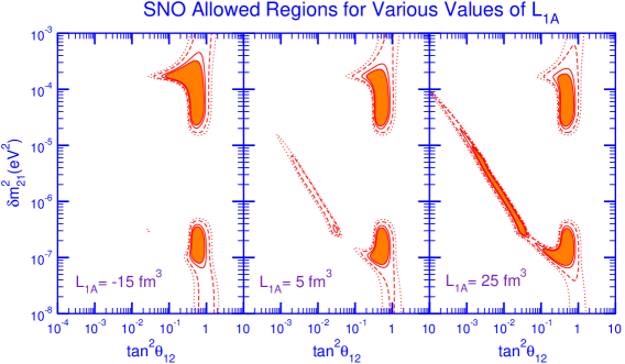
Figure 1: The change in the allowed region of the neutrino parameter space using solar neutrino data measured at SNO as the value of $L_{1A}$ changes. In the calculations leading to this figure the neutrino mixing angle $\theta_{13}$ is taken to be zero (see text). The shaded areas are the 90 % confidence level region. 95 % (solid line), 99 % (log-dashed line), and 99.73 % (dotted-line) confidence levels are also shown.

Helioseismic observation of the pressure-mode oscillations of the Sun can be used to put constraints on various inputs into the Standard Solar Model, in particular the $pp$ fusion cross section. This process has been calculated to the fifth order in pionless effective field theory Butler:2001jj . Neutrino-deuteron and antineutrino-deuteron scattering are computed to the third order in the same approach. The value of $L_{1A}$ is not the same in different orders. Helioseismology limits $L_{1A}=7.0\pm 5.9\>\mathrm{fm}^{3}$ in the fifth order Brown:2002ih . Using the expressions given in Ref. Butler:2002cw this gives

$$L_{1A}=4.8\pm 6.7\>\mathrm{fm}^{3}$$ (3)

in the third order. A state of the art calculation of the $pp$ fusion cross section was given in Schiavilla:1998je where the uncertainty in the axial two-body current operator was adjusted to reproduce the measured Gamow-Teller matrix element of tritium $\beta$ decay. After performing the transformation from the fifth- to third-order, the calculation of Ref. Schiavilla:1998je indicates a value of

$$L_{1A}=4.2\pm 2.4\>\mathrm{fm}^{3}.$$ (4)

One can also try to determine the counter term directly using the solar neutrino data. Using the Sudbury Neutrino Observatory (SNO) and SuperKamiokande (SK) charged-current, neutral current, and elastic scattering rate data Chen, Heeger, and Robertson (CHR) find Chen:2002pv

$$L_{1A}=4.0\pm 6.3\>\mathrm{fm}^{3}.$$ (5)

In order to obtain this result CHR wrote the observed rate in terms of an averaged effective cross section and a suitably defined response function. In this paper we explore the phenomenology associated with the variation of $L_{1A}$.

In our calculations we used the neutrino cross sections given in Refs. Butler:1999sv and Butler:2000zp . The radiative corrections are taken into account following Ref. Kurylov:2001av . To calculate observed solar neutrino rates and spectra we used a covariance approach the details of which are described in Ref. Balantekin:2003dc . In all calculations to obtain the MSW survival probabilities we used the neutrino spectra and solar electron density profile given by the Standard Solar Model of Bahcall and collaborators Bahcall:2000nu .

The dependence of the extracted neutrino parameters on the value of $L_{1A}$ is not very strong. We show how the parameter space changes with $L_{1A}$ in Figure 1. In this figure to find the allowed regions we fit 34 data points from the SNO day-night-spectrum Ahmad:2001an using the procedure of Ref. Balantekin:2003dc . The shaded area is the 90 % confidence level region. 95 % (solid line), 99 % (log-dashed line), and 99.73 % (dotted-line) confidence levels are also shown. As $L_{1A}$ changes from $-15\>\mathrm{fm}^{3}$ to $25\>\mathrm{fm}^{3}$ we note that the changes in the shape of the confidence level intervals are small. In the calculations leading to this figure we took the total ${}^{8}{\mathrm{B}}$ flux to be a free parameter using the procedure discussed in Ref. Balantekin:2003dc . (Note that even though we show the entire parameter space in this figure in the rest of this paper we concentrated in the large mixing angle region which is preferred by the global analysis). We conclude that the uncertainty in $L_{1A}$ can not be a significant source of error in the analysis of SNO data.

In general, both the deuteron breakup cross section and the total count rate at SNO are nonlinear in $L_{1A}$. Since $L_{1A}$ is small the charged- and neutral current count rates can be linearized by making a first order expansion, i.e.

$$\mathrm{Count}\,\mathrm{Rate}\sim A+B\,L_{1A},$$ (6)

as was done by CHR. Both the energy dependence and the overall magnitude of the ⁸B flux is an input into the Standard Solar Model. The energy dependence is rather accurately determined by the laboratory measurements of the ⁸B decay. The overall magnitude is determined by the measured rate of the ${}^{7}{\mathrm{Be}}(p,\gamma)^{8}{\mathrm{B}}$ reaction (for a review see Ref. Adelberger:1998qm ). To account for the sensitivity of the calculations on the value of the ⁸B flux we set $\Phi(^{8}{\mathrm{B})}=f_{B}\Phi_{\mathrm{SSM}}(^{8}{\mathrm{B})}$ and calculate the total rate for various values of the parameter $f_{B}$. Clearly the total count rate should be proportional to the value of $f_{B}$. Note that the elastic scattering count rate is independent of $L_{1A}$. Thus allowing $f_{B}$ vary freely cannot be fully compensated by changing $L_{1A}$ as we discuss below.

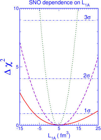
Figure 2: Projection of the global $\Delta\chi^{2}$ function on the parameter $L_{1A}$. In the calculations leading to this figure $\theta_{13}$ is taken to be zero. $\theta_{12}$, $\delta m_{12}^{2}$, and the parameter $f_{B}$ (the multiplier of the ⁸B flux) are varied. The solid line represents the case where all these three are unconstrained. The long-dashed line is when the ⁸B flux is fixed as described in the text, but the other two are unconstrained. The dotted line is when $\theta_{12}$ and $\delta m_{12}^{2}$ are also taken to be the best fit values to the SNO energy spectra.

In Figure 2 we present the quantity $\Delta\chi^{2}=\chi^{2}-\chi^{2}_{\rm min}$ calculated as a function of $L_{1A}$. In this figure $\Delta\chi^{2}$ is projected only on one parameter ($L_{1A}$) so that $n-\sigma$ bounds on it are given by $\Delta\chi^{2}=n^{2}$. $\theta_{13}$ is assumed to be zero. The solid line represents the case in which all other parameters ($\theta_{12}$, $\delta m_{12}^{2}$, and $f_{B}$) are unconstrained. The best fit value is given by $L_{1A}=4.5\>\mathrm{fm}^{3}$. In this case $L_{1A}$ is constrained between $-7\>\mathrm{fm}^{3}$ and $23\>\mathrm{fm}^{3}$ at $1\sigma$ level. Such a wide range is not surprising since the dependence of the rate on $L_{1A}$ is small and the effects of the parameters like $\theta_{12}$, $\delta m_{12}^{2}$, and $f_{B}$ are much more dominant. In order to obtain a better bound on $L_{1A}$, we fix $f_{B}$ so that the total count rate of SNO Ahmad:2001an is exactly reproduced at the value of $L_{1A}$ which corresponds to the minimum $\chi^{2}$ of the fit while the parameters $\theta_{12}$ and $\delta m_{12}^{2}$ are unconstrained. The resulting fit is shown by the dashed line. In this case $L_{1A}$ is constrained between $-2\>\mathrm{fm}^{3}$ and $13\>\mathrm{fm}^{3}$ at $1\sigma$ level. The dotted line in this figure represents the case where we fix all the parameters except $L_{1A}$. We find the best fit values of $\theta_{12}$ and $\delta m_{12}^{2}$ in a global fit using 93 data points from solar and reactor neutrino experiments; namely the total rate of the chlorine experiment (Homestake Cleveland:nv ), the average rate of the gallium experiments (SAGE Abdurashitov:2002nt , GALLEX Hampel:1998xg , GNO Altmann:2000ft ), 44 data points from the SK zenith-angle-spectrum Fukuda:2001nj , 34 data points from the SNO day-night-spectrum Ahmad:2001an and 13 data points from the KamLAND spectrum Eguchi:2002dm . In addition we fix $f_{B}$ so that the total count rate of SNO Ahmad:2001an is exactly reproduced. If we were to exclude SNO data from the global analysis and took $f_{B}=1$ instead of fixing as described above this method would be tantamount to treating SNO as an experiment to measure only $L_{1A}$ so that the uncertainties in the SNO data would only show up as the corresponding uncertainty at $L_{1A}$. From the dotted line $L_{1A}$ is constrained between $2\>\mathrm{fm}^{3}$ and $8\>\mathrm{fm}^{3}$ at $1\sigma$ level. In a sense this latter range represents the ”best case” limit on $L_{1A}$ that one can obtain from SNO. It is worth emphasizing that the $\chi^{2}$ minimum is almost the same in all these cases. In all cases we obtain a best fit value of $L_{1A}$ around $4.5$ to $5$ $\mathrm{fm}^{3}$ which is a little larger than the value obtained by CHR. These authors use elastic scattering, charged-current, and neutral-current rates separately with effective cross sections. Since we fit the solar neutrino day-night spectrum directly by folding differential cross sections, detector response functions, ${}^{8}{\mathrm{B}}$ spectrum, and the MSW survival probabilities we need a slightly larger $L_{1A}$.

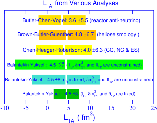
Figure 3: Values of $L_{1A}$ obtained from different analyses. The values labeled this work are calculated using the dashed and the dotted lines of Figure 2 as described in the text. Helioseismology limit is from Ref. Brown:2002ih . Reactor antineutrino limit is from Ref. Butler:2002cw . The limit obtained by CHS Chen:2002pv is also shown.

In Figure 3 we compare our results with results from other analyses. Our results are based on the dashed and dotted lines of Figure 2. We calculate $1\sigma$ errors by fitting a Gaussian of the form

$$\exp\left[-\frac{1}{2}\left(\frac{L_{1A}-L_{1A}^{\mathrm{average}}}{\sigma_{L_{1A}}}\right)^{2}\right]$$ (7)

to each side of the marginal likelihood expression $\mathcal{L}=\exp\left(-\Delta\chi^{2}/2\right)$ and estimate two standard deviations separately for each side bevrob . We obtain the error band shown in the figure by symmetrizing those errors.

One of the open questions in neutrino physics is understanding the role of mixing between the first and third flavor generations, $\theta_{13}$. In this regard we also explored if the uncertainties coming from the lack of knowledge of $\theta_{13}$ and the counter-term $L_{1A}$ are comparable. In the limiting case of small $\cos{\theta_{13}}$ and $\delta m_{31}^{2}\gg\delta m_{21}^{2}$, which seems to be satisfied by the measured neutrino properties, it is possible to incorporate the effects of $\theta_{13}$ rather easily. In this limit the three-flavor survival probability is is given by Kuo:1989qe ; Fogli:2000bk ; Balantekin:2003dc

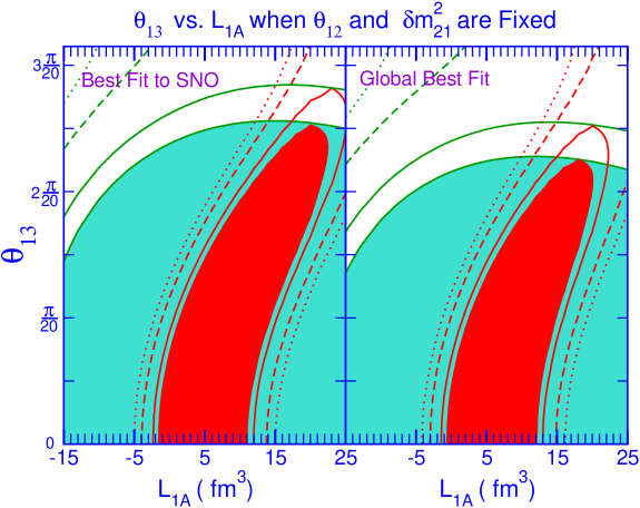
Figure 4: Allowed parameter space when $\theta_{12}$ and $\delta m_{12}^{2}$ are fixed to give the minimum $\chi^{2}$ values to reproduce the SNO day-night spectrum (left-hand panel) and all solar neutrino experiments along with the KamLAND experiment (right-hand panel). The shaded areas are the 90 % confidence level region. 95 % (solid line), 99 % (log-dashed line), and 99.73 % (dotted-line) confidence levels are also shown. The dark-shaded region corresponds to the case when the ⁸B flux is fixed to be the Standard Solar Model value. The light-shaded region corresponds to the case when that flux is unconstrained.

$$P_{3\times 3}(\nu_{e}\rightarrow\nu_{e}) = \cos^{4}{\theta_{13}}\>P_{2\times 2}(\nu_{e}\rightarrow\nu_{e}\>{\rm with}\>N_{e}\cos^{2}{\theta_{13}})$$ (8)

$$+\sin^{4}{\theta_{13}}.$$

In Eq. (8) the quantity $P_{2\times 2}(\nu_{e}\rightarrow\nu_{e}\>{\rm with}\>N_{e}\cos^{2}{\theta_{13}})$ is the standard two-flavor survival probability calculated with the modified electron density $N_{e}\cos^{2}{\theta_{13}}$ and the standard initial conditions. This suggests that for small values of $\theta_{13}$ the survival probability and consequently the counting rate can be linearized in $\cos^{4}{\theta_{13}}$:

$$\mathrm{Count}\,\mathrm{Rate}\sim A+B\,(1-\cos^{4}{\theta_{13}}).$$ (9)

The neutral- and charged-current counting rates linearly depend on $L_{1A}$ while elastic scattering rate does not. Conversely the charged-current and elastic scattering rates linearly depend on $\cos^{4}{\theta_{13}}$ while the neutral-current rate does not. Hence it is reasonable to compare their relative contributions. To this end in Figure 4 we show the allowed $\theta_{13}$ and $L_{1A}$ parameter space when $\theta_{12}$ and $\delta m_{12}^{2}$ are taken to give the minimum $\chi^{2}$ values to reproduce the data. Results where the fixed values of $\theta_{12}$ and $\delta m_{12}^{2}$ obtained using only the best fit of the SNO data (left-hand panel) and using the best fit of all the solar neutrino data along with KamLAND results (right-hand panel) are both shown. The dark-shaded region corresponds to the case when $f_{B}=1$. The light-shaded region corresponds to the case when the ⁸B flux is unconstrained. We observe that the uncertainty coming from the lack of a better knowledge of $\theta_{13}$ is larger than uncertainty coming from not knowing $L_{1A}$ precisely. One also observes that as $\theta_{13}$ increases the allowed $L_{1A}$ region shifts toward larger values of $L_{1A}$. When $\theta_{13}=0$ the electron neutrino flux is lost into only one channel: a particular linear combination of $\mu$ and $\tau$ neutrinos Balantekin:1999dx . But when $\theta_{13}\neq 0$ additional flux is lost into the orthogonal channel as well. The slightly decreased electron neutrino survival probability reduces the charged-current and the elastic scattering count rates so that a slightly larger $L_{1A}$ is needed to compensate the resulting decrease in the count rates at each bin.

In conclusion we showed that the SNO experiment with increased statistics using additional input from other solar neutrino experiments can significantly reduce the uncertainty in determining the precise form of the axial two-body currents at low energies. We also showed the contribution of the uncertainty in $L_{1A}$ to the analysis and interpretation of the SNO data is nearly negligible. The effect of this uncertainty is smaller than effects of a non-zero value of $\theta_{13}$ or even than effects of possible solar density fluctuations Balantekin:2003qm . Finally our most conservative value for $L_{1A}$ is significantly larger than that was obtained by CHR. One reason for this may be the treatment of neutral- and charged-current count rates together in the global analysis.

References

- (1) D. B. Kaplan, M. J. Savage and M. B. Wise, Phys. Lett. B 424, 390 (1998) [arXiv:nucl-th/9801034].
- (2) D. B. Kaplan, M. J. Savage and M. B. Wise, Phys. Rev. C 59, 617 (1999) [arXiv:nucl-th/9804032]; J. W. Chen, G. Rupak and M. J. Savage, Nucl. Phys. A 653, 386 (1999) [arXiv:nucl-th/9902056]; T. D. Cohen, Phys. Rev. C 55, 67 (1997) [arXiv:nucl-th/9606044]; P. F. Bedaque and U. van Kolck, Ann. Rev. Nucl. Part. Sci. 52, 339 (2002) [arXiv:nucl-th/0203055].
- (3) M. Butler and J. W. Chen, Nucl. Phys. A 675, 575 (2000) [arXiv:nucl-th/9905059].
- (4) M. Butler, J. W. Chen and X. Kong, Phys. Rev. C 63, 035501 (2001) [arXiv:nucl-th/0008032].
- (5) S. Ando, Y. H. Song, T. S. Park, H. W. Fearing and K. Kubodera, Phys. Lett. B 555, 49 (2003) [arXiv:nucl-th/0206001].
- (6) F. J. Kelly and H. Uberall, Phys. Rev. Lett. 16, 145 (1966).
- (7) S. D. Ellis and J. N. Bahcall, Nucl. Phys. A 114, 636 (1968).
- (8) S. Ying, W. Haxton and E. M. Henley, Phys. Rev. D 40, 3211 (1989).
- (9) N. Tatara, Y. Kohyama and K. Kubodera, Phys. Rev. C 42, 1694 (1990).
- (10) S. Ying, W. C. Haxton and E. M. Henley, Phys. Rev. C 45, 1982 (1992).
- (11) M. Doi and K. Kubodera, Phys. Rev. C 45, 1988 (1992).
- (12) S. Nakamura, T. Sato, V. Gudkov and K. Kubodera, Phys. Rev. C 63, 034617 (2001) [arXiv:nucl-th/0009012].
- (13) I. S. Towner, Phys. Rev. C 58, 1288 (1998).
- (14) J. F. Beacom and S. J. Parke, Phys. Rev. D 64, 091302 (2001) [arXiv:hep-ph/0106128].
- (15) A. Kurylov, M. J. Ramsey-Musolf and P. Vogel, Phys. Rev. C 65, 055501 (2002) [arXiv:nucl-th/0110051].
- (16) S. Nakamura, T. Sato, S. Ando, T. S. Park, F. Myhrer, V. Gudkov and K. Kubodera, Nucl. Phys. A 707, 561 (2002) [arXiv:nucl-th/0201062].
- (17) A. Kurylov, M. J. Ramsey-Musolf and P. Vogel, Phys. Rev. C 67, 035502 (2003) [arXiv:hep-ph/0211306].
- (18) M. Butler, J. W. Chen and P. Vogel, Phys. Lett. B 549, 26 (2002) [arXiv:nucl-th/0206026].
- (19) M. Butler and J. W. Chen, Phys. Lett. B 520, 87 (2001) [arXiv:nucl-th/0101017].
- (20) K. I. Brown, M. N. Butler and D. B. Guenther, arXiv:nucl-th/0207008.
- (21) R. Schiavilla et al., Phys. Rev. C 58, 1263 (1998) [arXiv:nucl-th/9808010].
- (22) J. W. Chen, K. M. Heeger and R. G. H. Robertson, Phys. Rev. C 67, 025801 (2003) [arXiv:nucl-th/0210073].
- (23) A. B. Balantekin and H. Yuksel, J. Phys. G: Nucl. Part. Phys. 29, 665 (2003). [arXiv:hep-ph/0301072].
- (24) J. N. Bahcall, M. H. Pinsonneault and S. Basu, Astrophys. J. 555, 990 (2001) [arXiv:astro-ph/0010346].
- (25) Q. R. Ahmad et al. [SNO Collaboration], Phys. Rev. Lett. 87, 071301 (2001) [arXiv:nucl-ex/0106015], Q. R. Ahmad et al. [SNO Collaboration], Phys. Rev. Lett. 89, 011302 (2002) [arXiv:nucl-ex/0204009]; Phys. Rev. Lett. 89, 011301 (2002) [arXiv:nucl-ex/0204008].
- (26) E. G. Adelberger et al., Rev. Mod. Phys. 70, 1265 (1998) [arXiv:astro-ph/9805121].
- (27) B. T. Cleveland et al., Astrophys. J. 496, 505 (1998).
- (28) J. N. Abdurashitov et al. [SAGE Collaboration], J. Exp. Theor. Phys. 95, 181 (2002) [Zh. Eksp. Teor. Fiz. 122, 211 (2002)] [arXiv:astro-ph/0204245].
- (29) W. Hampel et al. [GALLEX Collaboration], Phys. Lett. B 447, 127 (1999).
- (30) M. Altmann et al. [GNO Collaboration], Phys. Lett. B 490, 16 (2000) [arXiv:hep-ex/0006034].
- (31) S. Fukuda et al. [Super-Kamiokande Collaboration], Phys. Rev. Lett. 86, 5651 (2001) [arXiv:hep-ex/0103032], S. Fukuda et al. [Super-Kamiokande Collaboration], Phys. Rev. Lett. 86, 5656 (2001) [arXiv:hep-ex/0103033].
- (32) K. Eguchi et al. [KamLAND Collaboration], Phys. Rev. Lett. 90, 021802 (2003) [arXiv:hep-ex/0212021].
- (33) P.R. Bevington and D.K. Robinson, Data Reduction and Error Analysis for the Physical Sciences (McGraw-Hill, New York, 1992).
- (34) T. K. Kuo and J. Pantaleone, Rev. Mod. Phys. 61, 937 (1989).
- (35) G. L. Fogli, E. Lisi, D. Montanino and A. Palazzo, Phys. Rev. D 62, 113004 (2000) [arXiv:hep-ph/0005261].
- (36) A. B. Balantekin and G. M. Fuller, Phys. Lett. B 471, 195 (1999) [arXiv:hep-ph/9908465].
- (37) A. B. Balantekin and H. Yuksel, Phys. Rev. D 68, 013006 (2003) [arXiv:hep-ph/0303169].