Non-perturbative effects and the resummed Higgs transverse momentum distribution at the LHC
Anna Kulesza¹ and W. James Stirling²
1) Department of Physics, Brookhaven National Laboratory, Upton, NY 11973, U.S.A.

2) Institute for Particle Physics Phenomenology, University of Durham, Durham DH1 3LE, U.K.

Abstract

We investigate the form of the non-perturbative parameterization in both the impact parameter ($b$) space and transverse momentum ($p_{T}$) space resummation formalisms for the transverse momentum distribution of single massive bosons produced at hadron colliders. We propose to analyse data on $\Upsilon$ hadroproduction as a means of studying the non-perturbative contribution in processes with two gluons in the initial state. We also discuss the theoretical errors on the resummed Higgs transverse momentum distribution at the LHC arising from the non-perturbative contribution.

1. Introduction

The main discovery channel for a light Higgs boson at the future Large Hadron Collider (LHC) is the gluon-gluon fusion process $gg\rightarrow HX$. Studies of the production characteristics are of great importance for further understanding QCD and determining the Higgs parameters. A particularly interesting quantity is the transverse momentum ($p_{T}$) distribution of the produced Higgs boson. In particular, a precise knowledge of the Higgs $p_{T}$ distribution is important for determining an optimal set of cuts on the final state particles. In the past, the study of the transverse momentum distribution in Drell-Yan lepton pair and electroweak boson production helped to establish the validity of the soft gluon resummation formalism for the distribution at small $p_{T}$, and played an important part in determining the Standard Model (SM) electroweak parameters.

Reliable predictions for transverse momentum distributions at small $p_{T}$ can only be obtained if soft gluon emission effects are correctly taken into account. The soft radiation manifests itself in the presence of large logarithmic corrections in the theoretical expressions. The two prominent examples are recoil logarithms of the form $\alpha_{S}^{n}\ln^{(2n-1)}(Q^{2}/p_{T}^{2})$ and threshold logarithms of the form of $\alpha_{S}^{n}\ln^{(2n-1)}(1-z)/(1-z)$ (where $z=Q^{2}/\hat{s}$). A finite result can be recovered by resumming these corrections to all orders in $\alpha_{S}$. To date, the most studied method for resumming the recoil (or ‘Sudakov’) corrections in transverse momentum distribution for vector boson ($\gamma^{*}$, $Z$, $W$) production is the impact parameter ($b$, Fourier conjugate to $p_{T}$, space) formalism, also known as the Collins–Soper–Sterman (CSS) formalism [1]. Derived from the $b$ space resummation formalism are $p_{T}$ space methods [3, 4, 5], which not only provide a very good approximation of the $b$ space result but also avoid certain drawbacks related to the $b$ space method [3, 4]. As recently demonstrated, both the recoil and threshold corrections can be taken into account within the framework of the joint formalism [6, 7, 8].

The application of the CSS formalism to Higgs production at the LHC is a straightforward task and several analyses exist in the literature [9, 10, 11, 12]. One of the topics discussed here is the application of the $p_{T}$ space formalism to Higgs production at the LHC. Some preliminary results based on the $p_{T}$ space method have already been presented in Ref. [13].

The CSS formalism resums logarithms arising from arbitrarily soft gluon emission and therefore needs a prescription for dealing with the Landau pole. Originally this was incorporated by introducing an arbitrary (inverse energy) scale ($b_{*}$) above which the perturbatively calculated expression remained constant, i.e. ‘frozen’ at $b_{*}$. Additionally, a gaussian function, for example $\exp(-gb^{2})$ in its simplest form, was introduced to correct the formalism for non-perturbative effects at large $b$, i.e. intrinsic transverse momentum. The parameters of this function are in principle determined from experiment through fits to the data. In the case of Drell-Yan lepton pair or electroweak boson production, determining the size of the non-perturbative contribution associated with the incoming quarks can be done relatively precisely since there is a significant amount of experimental data available.

Other methods for dealing with the Landau singularity have also been proposed in the literature. The approach of [6, 7], initially developed for the joint formalism and later applied to the $b$ space formalism in [12], relies on performing the inverse Fourier transform from $b$ to $p_{T}$ space as an integral along a contour in the complex $b$ plane. It returns a well-defined resummed distribution for all nonzero values of $p_{T}$, even without introducing any extra non-perturbative function. It turns out, however, that some non-perturbative input is still needed to obtain a good description of the $Z$ production data at the Tevatron [7]. In another development of the $b$ space formalism, Qiu and Zhang [27] proposed a smooth extrapolation of the perturbative resummed cross section to push the Landau singularity to infinity.

A complete description of Higgs production within a resummation formalism also requires a prescription for dealing with the non-perturbative regime. While the $b_{*}$ prescription (or other prescriptions) for defining the non-perturbative regime can be kept the same, a different non-perturbative function is expected to describe intrinsic $k_{T}$ in the $gg$ channel. A common hypothesis is that the non-perturbative parameters for this ($gg$) channel can be determined by multiplying one of the parameters of the non-perturbative function for Drell-Yan ($q\bar{q}$) production by a factor of $C_{A}/C_{F}$, although to the best of our knowledge there is no rigorous theoretical basis for this procedure.

In this paper we calculate the Higgs transverse momentum distribution at the LHC using the $p_{T}$ space formalism. This method also needs a non-perturbative (gaussian) input function to account for the intrinsic $k_{T}$. In order to determine the non-perturbative coefficients we propose here to study transverse momentum distribution in $\Upsilon$ production process. We argue that the $(gg\to\ \Upsilon)$ hadroproduction provides valuable information on the amount of intrinsic $k_{T}$ carried by incoming gluons. The analysis begins by testing the existing forms of the non-perturbative parameterization for Drell-Yan production and the $C_{A}/C_{F}$ hypothesis in $b$ space. A similar study is then performed for the $p_{T}$ space formalism. We finish by considering (or, in the case of $b$ space analysis, re-examining) the effects of the non-perturbative function on Higgs transverse momentum distribution at the LHC, and draw some conclusions on the uncertainty in the prediction for the Higgs boson transverse momentum distribution arising from non-perturbative effects.

2. Theory

We begin by recalling basic formulae for both $b$ space and $p_{T}$ space formalisms. A brief review of non-perturbative parameterizations follows.

2.1. $b$ space

The $b$ space resummed part of the theoretical cross section for Higgs boson production through the gluon-gluon fusion in hadronic collisions $p\ p\rightarrow H+X$ has the following form, cf. [1]

$${d\sigma^{\rm res}\over dp_{T}^{2}\,dQ^{2}} = {\sigma_{0}\tau\pi}\delta(Q^{2}-m_{H}^{2})\int^{1}_{0}\,dx_{A}\,dx_{B}\,\delta\left(x_{A}x_{B}-{Q^{2}\over s}\right)\times$$

$${1\over 2}\int_{0}^{\infty}db\,b\,J_{0}(p_{T}b)\,\exp[{\cal S}(b_{*},Q)]\,F^{NP}(b,Q,x_{A},x_{B}){f}^{\prime}_{g/A}\left(x_{A},{b_{0}\over b_{*}}\right)\,{f}^{\prime}_{g/B}\left(x_{B},{b_{0}\over b_{*}}\right)\,,$$

with $\sigma_{0}={\sqrt{2}G_{F}\alpha_{S}^{2}(\mu)\over 576\pi}$, $\tau=Q^{2}/s$, $b_{0}=2\exp(-\gamma_{E})$, and where

$${\cal S}(b,Q^{2})=-\int_{b_{0}^{2}\over b^{2}}^{Q^{2}}\frac{d\bar{\mu}^{2}}{\bar{\mu}^{2}}\bigg{[}\ln\bigg{(}{Q^{2}\over\bar{\mu}^{2}}\bigg{)}A(\alpha_{S}(\bar{\mu}^{2}))+B(\alpha_{S}(\bar{\mu}^{2}))\bigg{]}\,,$$ (2)

$$A(\alpha_{S})=\sum^{\infty}_{i=1}\left(\frac{\alpha_{S}}{2\pi}\right)^{i}A^{(i)}\ ,\quad B(\alpha_{S})=\sum^{\infty}_{i=1}\left(\frac{\alpha_{S}}{2\pi}\right)^{i}B^{(i)}\,.$$ (3)

For the gluon-gluon fusion process [14, 15],

$$A^{(1)} = 2C_{A}\;,\qquad\qquad\qquad\quad B^{(1)}\;=\;-2\beta_{0}\;,$$

$$A^{(2)} = 2C_{A}\left[C_{A}\left(\frac{67}{18}-\frac{\pi^{2}}{6}\right)-\frac{10}{9}T_{R}N_{F}\right]\;,$$

$$B^{(2)} = C_{A}^{2}\left({23\over 6}+{22\over 9}\pi^{2}-6\zeta_{3}\right)+4C_{F}N_{F}T_{R}-C_{A}N_{F}T_{R}\left({2\over 3}+{8\pi^{2}\over 9}\right)-{11\over 2}C_{F}C_{A}\;,$$ (4)

and $\beta_{0}={11\over 6}C_{A}-{2\over 3}N_{F}T_{R}$.

The ‘modified’ parton distributions ${f}^{\prime}$ are related to the $\overline{\rm MS}$ parton distributions, $f$, by a convolution [1, 16, 17]

$$f^{\prime}_{g/H}(x,\mu)=\sum_{c}\int_{x}^{1}{dz\over z}\,C_{ga}\left({x\over z},\mu\right)f_{a/H}\left(z,\mu\right)\ ,$$ (5)

where

$$\qquad\qquad C_{ga}(z,\mu)=\sum^{\infty}_{i=0}\left(\frac{\alpha_{S}}{2\pi}\right)^{i}C_{ga}^{(i)}\,,$$

$$C_{gg}^{(0)}(z,\mu) = \delta(1-z)\,,\qquad\qquad\qquad\qquad\qquad\qquad\qquad\qquad C^{(0)}_{gq}(z,\mu)=0\,,$$

$$C^{(1)}_{gg}(z,\mu) = \delta(1-z)\left[{\alpha_{S}(\mu)\over 2\pi}\left(C_{A}{\pi^{2}\over 6}+{11\over 2}+\pi^{2}\right)\right]\,,\qquad\quad C^{(1)}_{gq}(z,\mu)={\alpha_{S}(\mu)\over 2\pi}C_{F}z\,.$$

The next-to-leading logarithm (NLL) accuracy requires knowledge of the $A^{(1)},\ B^{(1)},A^{(2)}$ and $C^{(0)}_{ga}$ coefficients; the coefficients $A^{(3)},\ B^{(2)}$ and $C^{(1)}_{ga}$ are of NNLL order.

The expression (LABEL:CSSform) provides a good description of the $p_{T}$ distribution at small $p_{T}$; for larger values of $p_{T}$ one needs to match the resummed result with the fixed order result. This is achieved by writing

$${d\sigma\over dp_{T}^{2}dQ^{2}}={d\sigma^{\rm res}\over dp_{T}^{2}dQ^{2}}+Y(p_{T},Q)$$ (6)

where $Y(p_{T},Q)$ is the difference between the fixed-order and resummed results expanded up to the order at which the fixed-order expression is considered.

The $b_{*}$ variable in (LABEL:CSSform) is defined as

$$b_{*}={b\over\sqrt{1+(b/b_{\rm lim})^{2}}}\,,\qquad\qquad b_{*}<b_{\rm lim}$$ (7)

which ensures that the resummed $b$ space expression is well-defined. The replacement of $b$ by $b_{*}$ in (LABEL:CSSform) prevents the argument of $\alpha_{S}$ from entering the non-perturbative regime by ‘freezing’ the perturbative contribution at a certain $b\sim b_{\rm lim}$.

Using renormalization group analysis arguments, in [1] a universal form of the non-perturbative function $F_{NP}$ was proposed:

$$F^{NP}(Q,b,x_{A},x_{B})=\exp\left[-h_{Q}(b)\ln\left({Q\over 2Q_{0}}\right)-h_{A}(b,x_{A})-h_{B}(b,x_{B})\right]\,,$$ (8)

where $Q_{0}$ is an arbitrary constant indicating the smallest scale at which perturbation theory is reliable, $Q_{0}\sim 1/b_{\rm lim}$. The functions $h_{Q},\ h_{a},\ h_{b}$ are to be extracted by comparing theoretical predictions with experimental data. As postulated in [1], the flavour dependence of $F^{NP}$ can be ignored. The $\ln(Q/Q_{0})$ dependence in (8) is required to balance the $Q$ dependence of the Sudakov factor $\exp{\cal S}$. In addition, $h_{Q}$ was proved to be universal and its leading $b^{2}$ behaviour at large $b$ is suggested by the analysis of the infrared renormalon contribution [21], as well as a recent analysis of the dispersive approach to power corrections [22].

However, the detailed form of the non-perturbative function $F_{ab}^{NP}(Q,b,x_{a},x_{b})$ has remained a matter of theoretical dispute. Early studies of fixed-target Drell-Yan experimental data, see e.g. [19], suggested that a Gaussian parameterization of an intrinsic $q_{T}$ distribution provided a good description of data in the low $p_{T}$ ($1-2$ GeV) regime. Motivated by this result, Davies et al. (DSW) [20] approximated the function $F^{NP}$ by

$$F^{NP}(Q,b,x_{A},x_{B})=\exp\left[-g_{2}b^{2}\ln\left({Q\over 2Q_{0}}\right)-g_{1}b^{2}\right]\,.$$ (9)

The $g_{1}$ parameter in (9) can be interpreted as a measure of the intrinsic transverse momentum, whereas $g_{2}$ represents a contribution coming from unresolved gluons with $k_{T}<Q_{0}$ as the structure functions evolve from scales ${\cal O}(Q_{0})$ to ${\cal O}(Q)$. Assuming (9), with a particular choice of $Q_{0}=2$ GeV, $b_{\rm lim}=0.5$ GeV^-1, and using the Duke-Owens parton distribution functions [23], the DSW analysis gave

$$g_{1}=0.15{\rm\,GeV}^{2},\quad\quad g_{2}=0.40{\rm\,GeV}^{2}\,.$$ (10)

An alternative parameterization, proposed by Ladinsky and Yuan (LY) [24], incorporates an additional dependence on $\tau=x_{a}x_{b}$

$$F^{NP}(Q,b,x_{A},x_{B})=\exp\left[-g_{2}b^{2}\ln\left({Q\over 2Q_{0}}\right)-g_{1}b^{2}-g_{1}g_{3}b\ln(100x_{A}x_{B})\right]\,.$$ (11)

Choosing $Q_{0}=1.6$ GeV, $b_{\rm lim}=0.5$ GeV^-1 and using the CTEQ2M parton distribution functions, the parameters in (11) were determined,

$$g_{1}=0.11^{+0.04}_{-0.03}{\rm\,GeV}^{2},\quad\quad g_{2}=0.58^{+0.1}_{-0.2}{\rm\,GeV}^{2},\quad\quad g_{3}=-1.5^{+0.1}_{-0.1}{\rm\,GeV}^{-1}\,.$$ (12)

Both parameterizations were reviewed in [25]. Using high-statistics samples of Drell-Yan and (CDF Tevatron Run 0) $Z$ production data, the values of the DSW parameters were updated,

$$g_{1}=0.24^{+0.08}_{-0.07}{\rm\,GeV}^{2},\quad\quad g_{2}=0.34^{+0.07}_{-0.08}{\rm\,GeV}^{2}\,,$$ (13)

and the LY parameters were found to be

$$g_{1}=0.15^{+0.04}_{-0.03}{\rm\,GeV}^{2},\quad\quad g_{2}=0.48^{+0.04}_{-0.05}{\rm\,GeV}^{2},\quad\quad g_{3}=-0.58^{+0.26}_{-0.20}{\rm\,GeV}^{-1}\,.$$ (14)

Recently, a new form of Gaussian parametrization with an $x$-dependent term, proportional to $b^{2}$ (as opposed to the term linear in $b$ in Eq. 11) has been proposed [26]:

$$F^{NP}(Q,b,x_{A},x_{B})=\exp\left[-g_{2}b^{2}\ln\left(Q\over 2Q_{0}\right)-g_{1}b^{2}+g_{1}g_{3}b^{2}\ln(100x_{A}x_{B}))\right]$$ (15)

to provide a good description of the low $Q$ Drell-Yan data and the CDF, D0 $Z$ data from Tevatron Run 0 and Run I. The values of the coefficients determined in [26] are:

$$g_{1}=0.21\pm 0.01\ {\rm GeV}^{2},\qquad\qquad g_{2}=0.68\pm 0.02\ {\rm GeV}^{2},\qquad\qquad g_{3}=-0.60^{+0.05}_{-0.04}\ {\rm GeV}^{2}.$$ (16)

In our analysis described in the following sections we choose to use the standard $b_{*}$ prescription for the CSS formalism. An essentially similar analysis of non-perturbative effects can be performed for the CSS formalism with different prescriptions presented in [6, 7, 12] and in [27, 11].

2.2. $p_{T}$ space

The resummed expression in $p_{T}$ space, corresponding to (LABEL:CSSform), has the following form [5]

$${d\sigma\over dp_{T}dQ^{2}} = \sigma_{0}\tau\pi\delta(Q^{2}-M_{H}^{2})\int_{0}^{1}\,dx_{A}\,dx_{B}\,\delta\left(x_{A}x_{B}-{Q^{2}\over s}\right)\times$$ (17)

$$\Bigg{\{}-{1\over p_{T\,*}}{dp_{T\,*}\over dp_{T}}\Sigma_{1}(p_{T\,*},Q)f^{\prime}_{g/A}(x_{A},p_{T\,*})\,f^{\prime}_{g/B}(x_{B},p_{T\,*})\tilde{F}^{NP}$$

$$+\Sigma_{2}(p_{T\,*},Q){dp_{T\,*}\over dp_{T}}{d\over dp_{T\,*}}\left[f^{\prime}_{g/A}(x_{A},p_{T\,*})\,f^{\prime}_{g/B}(x_{B},p_{T\,*})\right]\tilde{F}^{NP}$$

$$+\Sigma_{2}(p_{T\,*},Q)f^{\prime}_{g/A}(x_{A},p_{T\,*})\,f^{\prime}_{g/B}(x_{B},p_{T\,*}){d\over dp_{T}}\tilde{F}^{NP}\Bigg{\}}\,.$$

where

$$\Sigma_{2}(p_{T},Q) = \int_{0}^{\infty}dxJ_{1}(x)\exp[{\cal S}(x,p_{T},Q)]=\exp({\cal S}_{\eta})\sum_{N=1}^{\infty}\Bigg{(}{-\alpha_{S}(\mu^{2})A^{(1)}\over\pi}\Bigg{)}^{N-1}{1\over(N-1)!}$$ (24)

$$\times \sum_{m=0}^{N-1}{\left(\begin{array}[]{c}N-1\\ m\end{array}\right)}\sum_{k=0}^{N-m-1}{\left(\begin{array}[]{c}N-m-1\\ k\end{array}\right)}\sum_{l=0}^{N-m-k-1}{\left(\begin{array}[]{c}N-m-k-1\\ l\end{array}\right)}$$

$$\times \sum_{j=0}^{N-m-k-l-1}{\left(\begin{array}[]{c}N-m-k-l-1\\ j\end{array}\right)}\sum_{i=0}^{N-m-k-l-j-1}{\left(\begin{array}[]{c}N-m-k-l-j-1\\ i\end{array}\right)}$$ (29)

$$\times c_{2}^{m}c_{3}^{k}c_{4}^{l}c_{5}^{j}c_{6}^{i}c_{1}^{N-m-k-l-j-i-1}\tau_{N+m+2k+3l+4j+5i-1}\,,$$ (30)

and $\Sigma_{1}=-\,p_{T}\;\partial\Sigma_{2}\,/\partial p_{T}$. The factor ${\cal S}_{\eta}$ and the $c$ and $\tau$ coefficients are listed in [4].

We choose to incorporate the low energy effects using the form of the $p_{T}$ space non-perturbative function $\tilde{F}^{NP}$ advocated in [3],

$$\tilde{F}^{NP}=1-\exp{[-\tilde{a}\,p_{T}^{2}]}\,.$$ (31)

The role of this function is to account for the distribution in the very low $p_{T}$ region, and here we are assuming that the shape there is approximately gaussian. However, in order to combine this with the perturbative result, the latter needs to be ‘frozen’ or ‘switched off’ at some critical value of $p_{T}$ where the coupling $\alpha_{S}$ becomes large. A similar freezing is required in the $b$ space approach where the coupling is effectively $\alpha_{S}(1/b)$. In other words, in a similar fashion to the $b$ space method, we require not only (i) a form $\tilde{F}^{NP}$ for the distribution in the non-perturbative region, but also (ii) a prescription for moving smoothly from the perturbative to the non-perturbative region. One possibility for the latter is the ‘freezing’ prescription of [3],

$$p_{T\,*}=\sqrt{p_{T}^{2}+p_{T\,{\rm lim}}^{2}\exp{\left[-\frac{p_{T}^{2}}{p_{T\,{\rm lim}}^{2}}\right]}}\,.$$ (32)

which has the property

$$p_{T\,*}=\left\{\begin{array}[]{c}p_{T}\,,\qquad\qquad\qquad\quad p_{T}\gg p_{T\,{\rm lim}}\,,\\ p_{T\,{\rm lim}}\,,\qquad\qquad\quad\quad p_{T}\ll p_{T\,{\rm lim}}\,.\end{array}\right.$$ (33)

It is important to note that there are two pieces of information contained in this definition: the value of the limiting value $p_{T\,{\rm lim}}$ and the abruptness of the transition to this value. The use of a gaussian function in the definition (32), compared to say a power law function, implies a rapid transition from the perturbative to the non-perturbative region.

As noted earlier, the considerable amount of data on transverse momentum of colour singlets produced in processes with two initial quarks makes it possible to determine the non-perturbative function relatively precisely. This is not the case for the gluon initiated processes. In fact the only data available are on the transverse momentum distribution for low $Q$ resonance production. We argue here that E605 data on $\Upsilon$ hadroproduction [29] can provide useful information on the parameters of a non-perturbative function for processes with gluons in the initial state. At the values of $x_{F}$ where the cross section is measured, the $q\bar{q}$ contribution to $\Upsilon$ production can be neglected leaving only the $gg$ channel [28]. Moreover, we also argue that final state interactions do not introduce significant additional effects and therefore can be neglected. Since the final state interactions are expected to give rise to power corrections, their effects at values of $Q\sim m_{\Upsilon}$ relevant for $\Upsilon$ production are at the percent level of the total cross section. Consequently, the basic mechanisms responsible for $\Upsilon$ and Higgs production are similar. We will therefore assume that a good description of the transverse momentum in $\Upsilon$ production can be achieved with the help of the standard formulae for gluon initiated processes in $b$ or $p_{T}$ space, while allowing for an arbitrary overall normalization. We also assume that the major contribution to the measured cross section for $\Upsilon$ production comes from the 1S resonance with $m_{\Upsilon(1S)}=9.5$ GeV, and we therefore neglect the contributions from other resonances in our theoretical predictions.

3. Non-perturbative function in $b$ space

We begin our analysis by studying the non-perturbative function for the impact parameter formalism in $b$ space. We assume the standard value of the $b_{\rm lim}$ parameter, i.e. $b_{\rm lim}=0.5$ GeV^-1. The dependence of a form of the non-perturbative function on the $b_{\rm lim}$ parameter and correlations between the non-perturbative parameters and $b_{\rm lim}$ are not investigated here; a discussion of this issue can be found in [17].

Given the $\tau$-independent form of the non-perturbative function and the relatively narrow mass ranges of the data sets under consideration, the fitting procedure can be greatly simplified if one adopts an effective form for the non-perturbative function

$$F^{NP}=e^{-gb^{2}}$$ (34)

with $g$ an effective parameter, fitted separately for each of the $p_{T}$ distributions in the different mass bins. In this way one can test the dependence of the non-perturbative function on $Q$, and in particular possible departures from the proposed logarithmic dependence. Then, from the effective values of the non-perturbative parameters $g$ at different values of $Q$, the values of the non-perturbative parameters $g_{1}$ and $g_{2}$ and/or $g_{3}$ can be deduced. All fitting is done using the MINUIT fitting programme [35]. The resummed predictions fitted to data are accurate up to the NNLL level, but without including an available numerical estimate for the $A^{(3)}$ coefficient [37], the effect of which is known to be very small. The $Y$ term in (6) is taken at leading order. Since all the data analysed are at small $p_{T}$, the accuracy of matching does not play a significant role here. We use MRST2001 parton distribution functions [36] in all our theoretical predictions.

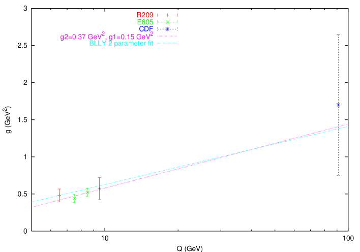
As a test of the fitting method using the effective function (34), we attempt to reproduce the values of the $g_{1},\ g_{2}$ parameters obtained by the BLLY collaboration [25]. We take exactly the same set of data as in Ref. [25], i.e. the first two mass bins ($7<Q<8$ GeV and $8<Q<9$ GeV) of the E605 data [29] (data with $p_{T}<1.4$ GeV), R209 data [30] ($p_{T}<2$ GeV) and CDF Run 0 data on $Z$ boson production [31] (data with $p_{T}<23$ GeV). The $p_{T}$ distribution measured by the R209 experiment in the $8<Q<11$ GeV bin was read off the plot in [25]. The authors of [17] pointed out the impact of the uncertainty in the normalization of the $p_{T}$ distributions on the determination of the non-perturbative parameters. Here we deal with the normalization uncertainty by simultaneously fitting multiple non-perturbative effective coefficients $g$ and one common normalization factor to data gathered in various different mass bins but coming from the same experiment. Given a set of effective coefficients $g$ for all mass bins considered, one can investigate its dependence on $Q$. There is evidence that $g$ increases slowly with $Q$, and in fact it is possible to fit a two-parameter function for the effective parameter $g$ as given by (9), i.e. $g=g_{2}\ln\left({Q/2Q_{0}}\right)+g_{1}$, to this data set. We obtain $g_{1}=0.15\pm 0.13\ {\rm GeV}^{2}$, $\ g_{2}=0.37\pm 0.14\ {\rm GeV}^{2}$, with $\chi^{2}/d.o.f.=0.33$. These values are within the error range of the BLLY values (13) and lead to effective coefficients $g$ for BLLY and our values of $g_{1},\;g_{2}$ being close to each other over the large range of $Q$, see Fig. 1.

Due to the method of fitting, our errors could be larger then the ones listed in [25]. The normalization factors for the theoretical predictions with respect to the experimental data for the E605 and R209 experiments are found to be $0.91\pm 0.07$ and $1.06\pm 0.09$ respectively, and are in good agreement with [25]. The normalization of the CDF $Z$ data from Run 0 is kept equal to one, as in [25]. All our fitting is done using the MINUIT fitting programme [35] and MRST2001 parton distribution functions [36]. Given the differences in the fitting method and the parton distribution functions being used, we interpret our ability to recover (within errors) the previously determined BLLY parameters as an indication that our fitting method can be used as a valuable diagnostic tool. The small value of $\chi^{2}/d.o.f$ may suggest that the errors on the effective parameters $g$ are overestimated.

Figure 1: Two-parameter fit to E605, R209 and CDF $Z$ data (Run 0) data samples chosen as in [25]

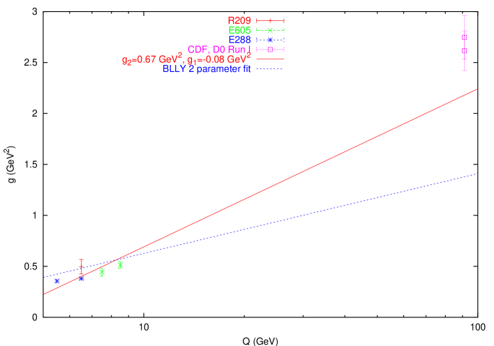
However, the BLLY fits were performed using data on $Z$ production gathered by the CDF collaboration [31] during Run 0 of the Tevatron $p\bar{p}$ collider. This particular data set has large statistical errors. The $p_{T}$ distribution for $Z$ production was measured much more accurately during Run I by both the CDF [33] and D0 [34] collaborations. A new analysis of the form of the non-perturbative function, including the Run I $Z$ data, appeared recently [26]. In agreement with the conclusions of [26], we find that the two-parameter form of the $F^{NP}$, given in Eq. 9, does not describe Run I data well, even after refitting for new values of parameters $g_{1}$ and $g_{2}$. In this analysis, in addition to CDF and D0 $Z$ data points with $p_{T}<20$ GeV, we take R209 [30] data points in the $5\;{\rm GeV}<Q<8\;{\rm GeV}$ bin only ($p_{T}<2$ GeV), E288 [32] data in the $5\;{\rm GeV}<Q<6\;{\rm GeV}$ and $6\;{\rm GeV}<Q<7\;{\rm GeV}$ bins ($p_{T}<2$ GeV, $\sqrt{s}=27.4$ GeV) and E605 [29] data in the $7\;{\rm GeV}<Q<8\;{\rm GeV}$ and $8\;{\rm GeV}<Q<9\;{\rm GeV}$ bins also with $p_{T}<2$ GeV. All points from CDF and D0 Run I data sets have $p_{T}<20$ GeV. Due to poor statistics, we do not include the Run 0 data. Because of known normalization discrepancies between the CDF and D0 experiments, normalization is allowed to be a free parameter while determining an effective parameter $g$ separately for each data set. For data from other experiments, values of effective $g$ parameters are determined in a fit which allows free normalization factor for theory predictions for each experiment, but these factors are kept the same for different $Q$ bins from the same experiment. The normalization factors (multiplicating theoretical results) are: $N_{E288}=0.81\pm 0.02,\ N_{E605}=0.90\pm 0.04,\ N_{R209}=1.1\pm 0.1,\ N_{CDF}=1.09\pm 0.02,\ N_{D0}=0.95\pm 0.03$. The fits of the $b$ space predictions to data return a set of effective $g$ coefficients for all mass bins considered, as shown in Fig. 2. A subsequent fit of the function $g=g_{2}\ln\left({Q/2Q_{0}}\right)+g_{1}$ to this set returns $g_{1}=-0.08\pm 0.09\ {\rm GeV}^{2}$, $g_{2}=0.67\pm 0.13\ {\rm GeV}^{2}$ with $\chi^{2}/d.o.f=8.25$. Fig. 2 illustrates the difference between an effective coefficient $g$ with these values of $g_{1},\;g_{2}$ and a coefficient $g$ with the BLLY values (10) as the function of $Q$.

Figure 2: Two-parameter fit to E288, E605, R209, CDF and D0 $Z$ (Run I) data samples chosen as described in text.

The BLNY parameterization (15) assumes a gaussian form of the non-perturbative function which includes dependence on $Q$ and $x$. To demonstrate this dependence in a clear fashion, it is convenient to rewrite the BLNY parametrization for the effective parameter $g$, cf. (15),

$$g=g_{1}+g_{2}\ln\left(Q\over 2Q_{0}\right)+g_{1}g_{3}\ln\left(100x_{A}x_{B}\right)\;,$$ (35)

in the form

$$g=g_{1}+g_{2}\ln\left(Q\over 2Q_{0}\right)+g_{3}\ln\left({\sqrt{s\over s_{0}\;}}\right)\;,$$ (36)

where we choose $\sqrt{s}_{0}=19.4$ GeV and $Q_{0}=1.6$ GeV. In effect, this parameterization introduces a $\sqrt{s}$ dependent component to $g_{1}$ in the two-parameter form of the $F^{NP}$ in Eq. 9. Apart from the sets of data mentioned above we also include in the fits testing (36) the E288 [32] data in the $5\;{\rm GeV}<Q<6\;{\rm GeV}$ and $6\;{\rm GeV}<Q<7\;{\rm GeV}$ bins ($p_{T}<2$ GeV) for two additional c.m. energies: $\sqrt{s}=19.4,\ 23.8$ GeV, as well as the E605 [29] data in the $10.5\;{\rm GeV}<Q<11.5$ GeV bin ($p_{T}<2$ GeV). All the data used in this analysis are contained in Table 1. Table 2 lists values of effective $g$ coefficients returned by the fits to the data. They are also plotted in Fig. 3. A subsequent fit of the function (36) to the set of these values reveals

$$g_{1}=0.12\pm 0.07\ {\rm GeV}^{2},\qquad\qquad g_{2}=0.22\pm 0.12\ {\rm GeV}^{2},\qquad\qquad g_{3}=0.29\pm 0.09\ {\rm GeV}^{2},$$ (37)

with $\chi^{2}/d.o.f=3.42$. The best fit normalization factors (multiplicating theoretical results) are listed in Table 2. Obviously, the quality of the fit improves after introducing a third parameter. The quoted value of $\chi^{2}/d.o.f$ also suggests that the choice of logarithmic dependence on $\sqrt{s}$ in Eq. 36 could be too simplified.

Translating the values of the $g_{1},\ g_{2}$ and $g_{3}$ parameters above to the BLNY non-perturbative function parameters (35) leads to

$$g_{1}=0.26\pm 0.1\ {\rm GeV}^{2},\qquad\qquad g_{2}=0.51\pm 0.07\ {\rm GeV}^{2},\qquad\qquad g_{3}=-0.55\pm 0.011\ {\rm GeV}^{2},$$ (38)

These values (with the exception of $g_{2}$) lie within the error band of the parameters determined by the BLNY collaboration. Note, however, that we use a different fitting technique as well as different data samples for the analysis.

Experiment	$\sqrt{s}$ (GeV)	$Q$ range (GeV)	$p_{T}$ range (GeV)
E605	38.8	7-9, 10.5-11.5	$0-2$
E288	19.4, 23.8, 27.4	5-7	$0-2$
R209	62	5-8	$0-2$
CDF	1800	91.2	$0-20$
D0	1800	91.2	$0-20$

Table 1: List of data used in the three-parameter analysis.

Experiment	$\sqrt{s}$ (GeV)	$Q$ range (GeV)	effective $g\;({\rm GeV}^{2})$	Normalization	$\chi^{2}/d.o.f$
E605	38.8	7-8	0.414 $\pm$ 0.047	0.842 $\pm$ 0.029	3.126
		8-9	0.472 $\pm$ 0.029
		10.5-11.5	0.517 $\pm$ 0.038
E288	19.4	5-6	0.273 $\pm$ 0.028	0.807 $\pm$ 0.020	1.680
		6-7	0.296 $\pm$ 0.031
	23.8	5-6	0.303 $\pm$ 0.029
		6-7	0.357 $\pm$ 0.038
	27.4	5-6	0.354 $\pm$ 0.024
		6-7	0.379 $\pm$ 0.146
R209	62.0	5-8	0.496 $\pm$ 0.071	1.103 $\pm$ 0.096	1.515
CDF	1800	91.2	2.746 $\pm$ 0.212	1.090 $\pm$ 0.022	0.509
D0	1800	91.2	2.615 $\pm$ 0.193	0.954 $\pm$ 0.025	0.911

Table 2: Effective $g$ coefficients from fits of $b$ space theoretical predictions to data.

Figure 3: Three-parameter fit to E288, E605, R209, CDF and D0 $Z$ (Run I) data samples chosen as described in text. The parallel lines correspond to non-perturbative function of the form (36) with coefficients (37) and values of $\sqrt{s}$ of each experiment analysed. The line marked ’BLNY’ corresponds to the BLLY fit of the form (15) with coefficients (16) at $\sqrt{s}=38.8$ GeV.

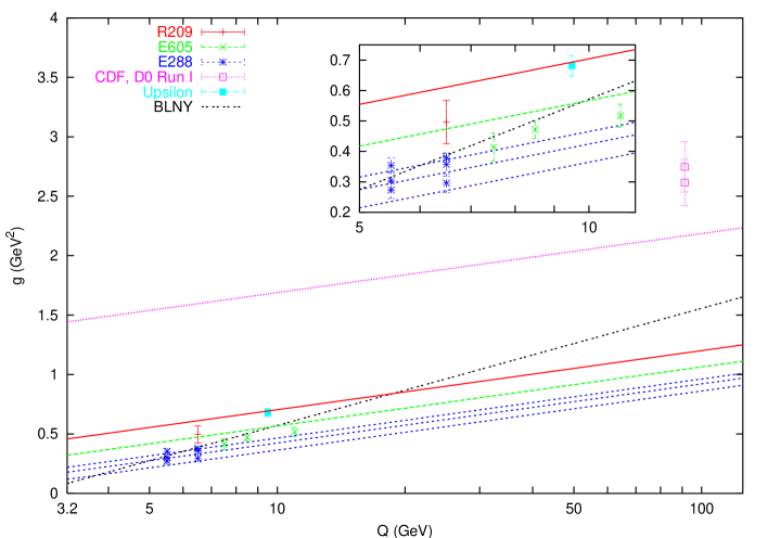
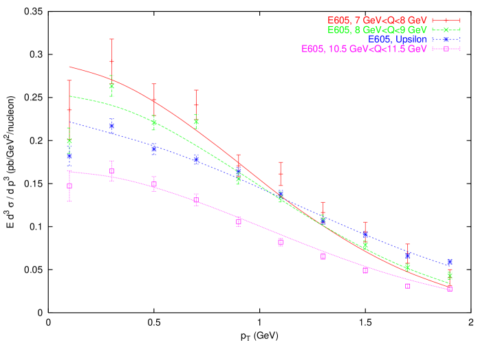
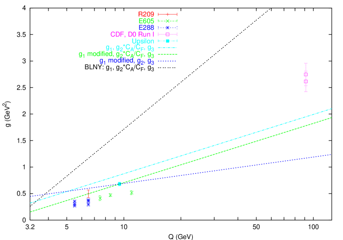
We next turn our attention to the non-perturbative function for the case of Higgs production via gluon-gluon fusion, where the transverse momentum of the Higgs particle at small values of $p_{T}$ is a result of soft gluon emission off the initial-state gluon lines. In our analysis we use E605 data for $\Upsilon$ $(pN)$ hadroproduction, allowing the normalization to be a free parameter fitted to data together with the non-perturbative parameters. We find the value of the effective parameter $g(\Upsilon)=0.68\pm 0.03\ {\rm GeV}^{2}$ with $\chi^{2}/d.o.f=2.79$. Interestingly, this is relatively close to the values of $g$ for the corresponding $q\bar{q}$ Drell-Yan production process with invariant masses of the same order of magnitude, cf. Fig. 3. This conclusion is not unexpected, given the similar shapes of the $p_{T}$ distributions for Drell-Yan and $\Upsilon$ production data, see Fig. 4.

Figure 4: E605 Drell-Yan (7 GeV$<Q<$8 GeV, 8 GeV$<Q<$9 GeV, 10.5 GeV$<Q<$11.5 GeV bins) and $\Upsilon$ data compared to theoretical predictions using the best three-parameter fit. In order to better compare the shapes of the $p_{T}$ distribution, the Drell Yan data have been rescaled by the factor of 0.3, 0.6, 2.1 for the 7 GeV$<Q<$8 GeV, 8 GeV$<Q<$9 GeV and 10.5 GeV$<Q<$11.5 GeV bins in $Q$, respectively.

The small difference between the values of $g$ for Upsilon and Drell-Yan production suggests that the common prescription of multiplying the D-Y coefficient $g_{2}$ by a factor $C_{A}/C_{F}$ for gluon-initiated processes might require adjustments in the values of the other coefficients in order to maintain the quality of the fit. This is illustrated in Fig. 5, where apart from the effective values of $g$ plotted for the analysed mass bins, we also plot the fitted effective $g$ at $\sqrt{s}=\sqrt{s}_{\rm E605}=38.8$ GeV, (35) and (36), with their coefficients $g_{2}$, as listed in (16) and (37), multiplied by the factor $C_{A}/C_{F}$. The significant difference between the two predictions originates not only in the different values of the $g_{2}$ coefficient obtained in our and the BLNY fits, but also from the different role of the $g_{2}$ coefficient itself – in our case (36) it solely measures the dependence on $Q$, whereas in (15) there is additional $Q$ dependence in the coefficients $g_{1}$ and $g_{3}$ through the relation $x_{1}x_{2}=Q^{2}/s$. As mentioned earlier, to bridge the gap between experiment and theory some other modifications to the values of the non-perturbative parameters will be needed in addition to the $C_{A}/C_{F}$ prescription. In particular, one may argue that while the $g_{3}$ parameter should stay the same in the non-perturbative functions relevant to processes with $q\bar{q}$ and $gg$ initial states, the $g_{1}$ coefficient can vary depending on the initial state. The universality of the $g_{3}$ coefficient can be motivated by general arguments for the logarithmic dependence on $\sqrt{s}$ for the contributions to the $p_{T}$ of the final state from fluctuations in the underlying event. Figure 5 shows the non-perturbative function (36) at $\sqrt{s}=\sqrt{s}_{\rm E605}=38.8$ GeV with $g_{1}$ modified to obtain $g=g(\Upsilon)$ both when $g_{2}$ is multiplied by $C_{A}/C_{F}$ and when it is left unchanged. The corresponding values of the ‘adjusted’ $g_{1}$ parameter are $g_{1}=-0.05\pm 0.4\ {\rm GeV}^{2}$ for the former and $g_{1}=0.24\pm 0.23\ {\rm GeV}^{2}$ for the latter model. Consequently, the range of allowed values of the effective parameter $g$ is rather large in each non-perturbative model discussed above. Moreover, since at the present time it is difficult to discriminate between the various models experimentally, the values of $g$ from all reasonable models are allowed. A band of allowed values of the effective parameters $g$ obtained in this way can be viewed as a useful estimate of the theoretical error in the $p_{T}$ distribution due to the non-perturbative input.

Figure 5: Drell-Yan (E288, E605, R209), Z production (CDF and D0 Run 1) and E605 Upsilon data together with the three-parameter fits, (15) and (36) at $\sqrt{s}=38.8$ GeV, with coefficients (16) and (37) modified as discussed in text.

4. Non-perturbative function in $p_{T}$ space

In general, the analysis of the non-perturbative function for the $p_{T}$ space resummation method follows the $b$ space analysis described in the previous section, except for the additional dependence of the non-perturbative function on the parameter $p_{T\,{\rm lim}}$. The value of this $p_{T}$ space parameter is a priori unknown, and its determination requires simultaneous fitting alongside the other non-perturbative parameters. In $b$ space, the analogous parameter $b_{\rm lim}$ is traditionally fixed at a value of 0.5 GeV^-1. The dependence of the resummed distributions for Drell-Yan production on the parameter $b_{\rm lim}$ has been studied in [17]. In general, varying the $b_{\rm lim}$ parameter will result in larger errors on the effective parameters $g$, and consequently on the transverse momentum distribution itself. In the $p_{T}$ space case, all the fits we perform are fits for the effective $\tilde{a}$ parameters (assumed different for each data set), the normalization factors (assumed identical for data which come from the same experiment but have different $Q$) and the factor $p_{T\,{\rm lim}}$ (assumed the same for all data sets). In fits for the $p_{T}$ space non-perturbative parameterization we use the same data sets and number of data points as in the $b$ space fits.

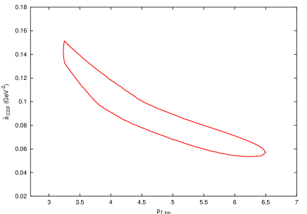
From a simultaneous fit to low $Q$ Drell-Yan and Run I $Z$ production data, we establish the value of $p_{T\,{\rm lim}}$ to be $p_{T\,{\rm lim}}=5.5\pm 2.98$ GeV with $\chi^{2}/d.o.f=1.54$. The value of $p_{T\,{\rm lim}}$ is strongly correlated with the normalization factors for the low $Q$ experiments and the value of $\tilde{a}$ for $Z$ production data, see Fig. 6. The normalization factors listed in Table 3 are different from their $b$ space counterparts. The effective parameters $\tilde{a}$ for all $Q$ bins are now determined in one fit which also determines the common factor $p_{T\,{\rm lim}}$. In the $b$ space analysis, the effective parameters $g$ for each $Q$ bin resulted from separate fits for all experiments – we did not fit for a common factor $b_{\rm lim}$. The resulting value of $p_{T\,{\rm lim}}$ appears rather large, if interpreted as defining the border between perturbative and non-perturbative physics.

Figure 6: The 68% C.L. contour in the $p_{T\,{\rm lim}}$, $\tilde{a}_{\;CDF}$ plane.

Motivated by the form of the three-parameter non-perturbative function (36) in $b$ space, we propose the following form for the dependence of the effective non-perturbative parameter $\tilde{a}$ on $Q$ in (31):

$$\tilde{a}=\left(\tilde{a}_{1}+\tilde{a}_{2}\ln\left(\frac{Q}{2Q_{0}}\right)+\tilde{a}_{3}\ln\left(\sqrt{\frac{s}{s_{0}}}\right)\right)^{-1}$$ (39)

As for the $b$ space analysis, we first fit the theoretical predictions to data in order to determine the effective coefficients $\tilde{a}$ for all mass bins analysed. A fit of (39) to the set of effective values of $\tilde{a}$, listed in Table 3 and shown in Fig. 7, returns the following values for the parameters:

$$\tilde{a}_{1}=0.20\pm 0.50\;{\rm GeV}^{-2},\qquad\qquad\tilde{a}_{2}=0.95\pm 0.92\;{\rm GeV}^{-2},\qquad\qquad\tilde{a}_{3}=1.56\pm 0.57\;{\rm GeV}^{-2},$$ (40)

with $\chi^{2}/d.o.f=1.38$. The errors on the coefficients are substantially larger than the corresponding errors on the coefficients in $b$ space, again due to the much larger number of parameters (i.e., the effective values of $\tilde{a}$ for bins in $Q$) determined in a single fit in the $p_{T}$ space analysis as compared to the $b$ space fits. In Fig. 7 we also plot the non-perturbative parameterization (39) for the $\sqrt{s}$ of each experiment analysed here, and the best fit coefficients $\tilde{a}_{1},\tilde{a}_{2},\tilde{a}_{3}$ listed above. As for $b$ space, the three parameter fit provides a much better description of the data than the two parameter case.

Experiment	$\sqrt{s}$ (GeV)	$Q$ range (GeV)	effective $\tilde{a}\;({\rm GeV}^{-2})$	Normalization	$\chi^{2}/d.o.f$
E605	38.8	7-8	0.645 $\pm$ 0.149	0.928 $\pm$ 0.067	1.552
		8-9	0.558 $\pm$ 0.072
		10.5-11.5	0.523 $\pm$ 0.079
E288	19.4	5-6	1.182 $\pm$ 0.216	0.991 $\pm$ 0.050
		6-7	1.014 $\pm$ 0.219
	23.8	5-6	0.998 $\pm$ 0.149
		6-7	0.865 $\pm$ 0.149
	27.4	5-6	0.773 $\pm$ 0.080
		6-7	0.721 $\pm$ 0.047
R209	62.0	5-8	0.529 $\pm$ 0.252	1.141 $\pm$ 0.288
CDF	1800	91.2	0.070 $\pm$ 0.012	1.050 $\pm$ 0.065
D0	1800	91.2	0.070 $\pm$ 0.013	0.914 $\pm$ 0.072

Table 3: Effective coefficients $\tilde{a}$ from fits of the $p_{T}$ space theoretical predictions to data.

Figure 7: Effective parameters $\tilde{a}$ for the Drell-Yan (E288, E605, R209), Z production (CDF and D0 Run 1) and E605 Upsilon data and the non-perturbative parameterization (39), together with the best fit values of coefficients (40) plotted for the $\sqrt{s}$ of each set of experimental data analysed.

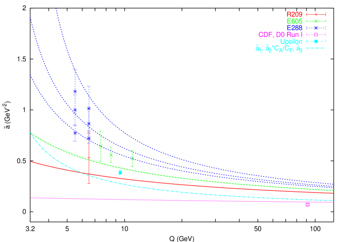
Given the $b$ space results for the fit to the $\Upsilon$ data, we would expect the effective parameter $\tilde{a}$ for $\Upsilon$ production to be relatively close to the corresponding values of $\tilde{a}$ for Drell-Yan production. This is indeed the case, as can be seen from Fig. 7. The fitted $\tilde{a}$ value for Upsilon production is $\tilde{a}(\Upsilon)=0.39\pm 0.02$ GeV^-2 ($\chi^{2}/d.o.f.=2.70$). The value of $\tilde{a}(\Upsilon)$ is determined from a simple fit to the $p_{T}$ distribution data where the only other quantity fitted is the overall normalization; $p_{T\,{\rm lim}}$ is kept fixed at the value determined from the fits to the DY data and the error on $p_{T\,{\rm lim}}$ is not taken into account. The resulting error on the fitted value of $\tilde{a}(\Upsilon)$ is therefore superficially small. Nevertheless, it remains true that the central value of the effective $\tilde{a}(\Upsilon)$ is closer to the value predicted by the non-perturbative parametrization (39) with (40) than by the same parameterization with the $\tilde{a}_{2}$ coefficient multiplied by $C_{A}/C_{F}$ – the equivalent of the $b$ space prescription of rescaling the $g_{2}$ coefficient by $C_{A}/C_{F}$. It therefore becomes an attractive alternative to consider other possible modifications to the values of the non-perturbative parameters, determined for the Drell-Yan type processes, to describe processes with gluons in the initial state. Following the $b$ space analysis presented in the previous section, we make the choice of adjusting the $\tilde{a}_{1}$ parameter while keeping $\tilde{a}_{3}$ unchanged and the parameter $\tilde{a}_{2}$ either unchanged or rescaled by $C_{A}/C_{F}$. The resulting values of the parameter $\tilde{a}_{1}$ are: $\tilde{a}_{1}=0.47^{+1.53}_{-1.52}$ GeV^-2 and $\tilde{a}_{1}=-0.82^{+2.78}_{-2.77}$ for the former and latter model, respectively. The magnitude of the errors is a straightforward consequence of the large errors on the effective parameters $\tilde{a}$ for the bins in $Q$.

5. The Higgs transverse momentum distribution in the $p_{T}$ space formalism

As discussed previously, in the resummation framework the $p_{T}$ distribution for the gluon-fusion induced Higgs production process is obtained assuming that the non-perturbative contribution has the same form as the non-perturbative function for Drell-Yan type processes — but with the $g_{2}$ or a corresponding parameter rescaled by a factor of $C_{A}/C_{F}$. The results presented in the previous two sections may suggest exercising some caution when applying this hypothesis.

In this section we focus on the effect of the non-perturbative function on predictions for the Higgs $p_{T}$ distribution, in both the $b$ space and $p_{T}$ space approach. In addition, we discuss the changes made to the coefficients of the non-perturbative function(s) to allow for gluons in the initial state and the impact of these modifications on the predictions for the Higgs $p_{T}$ distribution.

First, we focus on the $b$ space non-perturbative function. As can be seen from Fig. 8, the central values of the effective parameters $g$ for $\sqrt{s}=14$ TeV are rather close to each other, irrespective of the different treatments of the $g_{1},\;g_{2},\;g_{3}$ coefficients discussed above. However, the significant errors on the coefficients $g_{1}$, $g_{2}$ and $g_{3}$ result in an even more pronounced error on the effective parameter $g$ in each model. The errors are larger in models in which the $g_{2}$ coefficient is rescaled by $C_{A}/C_{F}$, as the errors get rescaled together with the central values. If we assume the mass of the Higgs boson to be $M_{H}=125$ GeV, the effective values are: $g=3.82\pm 1.66\ {\rm GeV}^{2}$ for the model with $g_{2}$ rescaled by $C_{A}/C_{F}$ and $g_{1}$, $g_{3}$ unchanged, $g=3.65\pm 1.99\ {\rm GeV}^{2}$ for the model with $g_{2}$ rescaled by $C_{A}/C_{F}$, $g_{1}$ modified and $g_{3}$ unchanged, $g=2.96\pm 1.25\ {\rm GeV}^{2}$ for the model with $g_{2}$, $g_{3}$ unchanged and $g_{1}$ modified. The next step is to implement the non-perturbative function (34) with these effective values of $g$ into the resummed formalism. Again, we view the spread in the central values of $g$ due to various models, together with the error bands on $g$ in each model, as a measure of the theoretical error on the effective parameter $g$. Consequently, we present the Higgs $p_{T}$ distributions for the smallest and the largest value of $g$ allowed by the error bands for all models. These values both happen to come from the model with $g_{2}$ rescaled by $C_{A}/C_{F}$, $g_{1}$ modified and $g_{3}$ unchanged, and correspond to $g=1.67\ {\rm GeV}^{2}$ and $g=5.64\ {\rm GeV}^{2}$.

Figure 10 shows the predicted transverse momentum distribution of the Higgs boson at the LHC calculated in the framework of the standard $b$ space resummation with the effective non-perturbative parametrization of the form (34) for two ‘extreme’ values of $g$ listed above. The resummed predictions are accurate up to NNLL level, i.e. they include the NNLL coefficients $C^{(1)},\;B^{(2)}$ as well as a numerical estimate of the coefficient $A^{(3)}$ [37], rescaled by $C_{A}/C_{F}$. The matching is performed at the leading-order level. We assume $M_{H}=125$ GeV and use MRST2001 parton distribution functions. We find, in agreement with Ref. [10, 11], only a very small dependence of the theoretical predictions on the exact values of the non-perturbative parameters. The predictions shown in Fig. 10 are somewhat lower than the ones presented in [12] but higher then those obtained in [11].

Figure 8: The effective parameter $g$ as a function of $Q$ in various models of the non-perturbative parametrization in $b$ space at $\sqrt{s}=14$ TeV. The central values are denoted by thick lines; the errors bands by thin lines. The dotted vertical line is drawn for $Q=125$ GeV.

Figure 9: The effective parameter $\tilde{a}$ as a function of $Q$ in various models of the non-perturbative parametrization in $p_{T}$ space at $\sqrt{s}=14$ TeV. The central values are denoted by thick lines; the errors bands by thin lines. The dotted vertical line is drawn for $Q=125$ GeV.

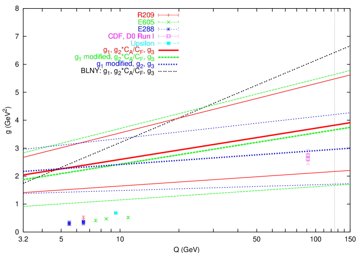
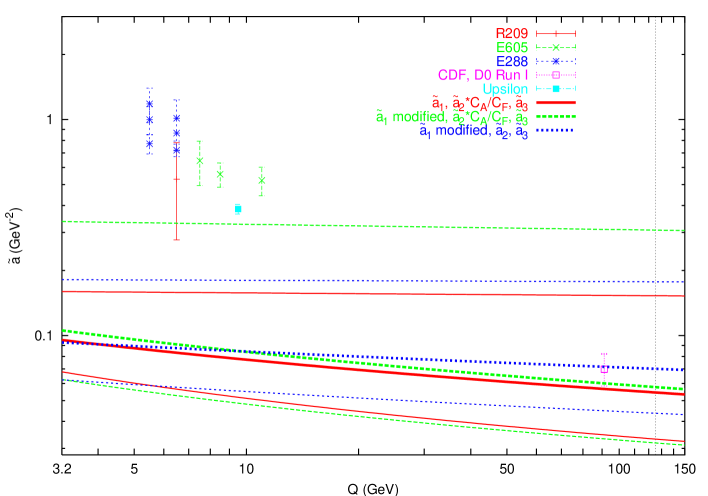
Analogously to $b$ space, the central values of the $p_{T}$-space parameter $\tilde{a}$, as predicted by the different models for $\sqrt{s}=14$ TeV and $M_{H}=125$ GeV, lie relatively close to each other, see Fig. 9. However, due to the large errors on the central values of $\tilde{a}$ associated with each model, the range of possible values of $\tilde{a}$ is an order of magnitude large. The central values (for $M_{H}=125$ GeV) are: $\tilde{a}=0.054^{+0.098}_{-0.021}$ GeV^-2 for the model with $\tilde{a}_{2}$ rescaled by $C_{A}/C_{F}$ and $\tilde{a}_{1}$, $\tilde{a}_{3}$ unchanged, $\tilde{a}=0.058^{+0.250}_{-0.026}$ GeV^-2 for the model with $\tilde{a}_{2}$ rescaled by $C_{A}/C_{F}$, $\tilde{a}_{1}$ modified and $\tilde{a}_{3}$ unchanged, $\tilde{a}=0.070^{+0.107}_{-0.026}$ GeV^-2 for the model with $\tilde{a}_{2}$, $\tilde{a}_{3}$ unchanged and $\tilde{a}_{1}$ modified. The smallest and largest values of $\tilde{a}$ also happen to come from the model with $\tilde{a}_{2}$ rescaled by $C_{A}/C_{F}$, $\tilde{a}_{1}$ modified and $\tilde{a}_{3}$ unchanged, and are: $\tilde{a}=0.032$ GeV^-2 and $\tilde{a}=0.308$ GeV^-2.

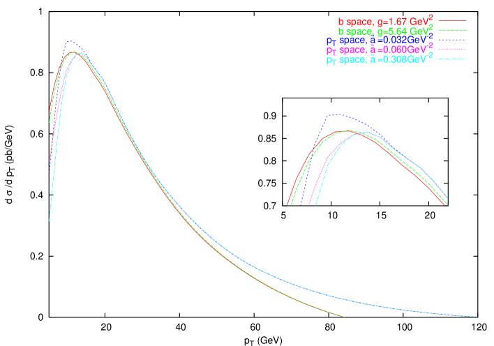
The Higgs transverse momentum distribution obtained in the framework of the $p_{T}$ space formalism is compared to the $b$ space results in Fig. 10. The $p_{T}$ space distribution is calculated assuming the effective non-perturbative function of the form (31) with a coefficient $\tilde{a}=0.06$ GeV^-2 and the best fit value of $p_{T\,{\rm lim}}=5.5$ GeV. The value of $\tilde{a}=0.06$ GeV^-2 is an average of the central values of $\tilde{a}$ in the various models of treating the $\tilde{a}_{1},\;\tilde{a}_{2},\;\tilde{a}_{3}$ coefficients discussed above. The $p_{T}$ space prediction agrees reasonably well with the $b$ space prediction in the small $p_{T}$ regime. The gap between the locations of the peaks of the distributions gets narrower for smaller values of $p_{T\,{\rm lim}}$ as well as smaller values of $\tilde{a}$. At larger values of $p_{T}$, the predictions of the two formalisms differ substantially. It is well known that the $b$ space distribution, even after matching with the fixed-order result, is eventually going to turn negative at sufficiently large $p_{T}$. This happens because the matching relies on the perturbative fixed-order result, known up to a certain order in $\alpha_{S}$. At one order higher than the matching accuracy, the resummed expression introduces logarithmic terms which will not be cancelled by the terms coming from the matching term $Y$ in (6). Since here matching is performed only at the LO level, the negative behaviour of the matched resummed distribution at large $p_{T}$ is quite pronounced. In the numerical realisation of the $p_{T}$ space method, only a subset of subleading higher order terms is summed. Consequently, the matched resummed distribution becomes negative at much larger values of $p_{T}$, increasing the range of applicability of the resummation approach.

As the analytic results for the NLO $p_{T}$ Higgs distribution are available in the literature [38], it is possible to improve the accuracy of results presented here by performing matching at the NLO. However, our main goal here is to (re-)examine the influence of the non-perturbative function on the $p_{T}$ distribution and for that purpose we consider the LO matching sufficient. The NNLL resummed $b$ space resulted matched to the NLO fixed-order expression was recently obtained in [12]. The problem of the negative large $p_{T}$ behaviour is normally solved by simply switching from the matched resummed cross section to the fixed order cross section (at an appropriate value of $p_{T}$) to obtain the cross section valid at all $p_{T}$.

At low values of $p_{T}$, the $b$ space predictions for the two choices of $g$ values are close to each other, in agreement with the conclusions of Ref. [10, 11]. The effect of changing the non-perturbative part is felt, albeit slightly, at all values of $p_{T}$. In contrast, all the predictions from the $p_{T}$ space formalism are already equal at $p_{T}\sim 15$ GeV. Around this value, the $p_{T}$ space formalism begins to return a ‘pure’ perturbative part (the Sudakov factor) without any non-perturbative contamination. It is clear from Eq. 17, that for $p_{T}\gg p_{T\,{\rm lim}}$ and in the limit $\tilde{a}\rightarrow\infty$ the $p_{T}$ space expression for the resummed cross section has only purely perturbative content. In the region of $p_{T}$ where the $p_{T}$ space predictions differ, the dependence on the values of the effective non-perturbative parameter $\tilde{a}$ is, however, much stronger than the analogous dependence on the parameter $g$ in $b$ space. For lower values of $\tilde{a}$ than the central value $\tilde{a}=0.06$ GeV^-2, the position of the peak and the value of the distribution at the peak changes significantly. In the case of the lower value of $\tilde{a}=0.032$ GeV^-2 the value of the distribution at the peak is around 5% larger than the corresponding value for $\tilde{a}=0.06$ GeV^-2 and the peak location moves by about 4 GeV towards smaller values of $p_{T}$. For values of $\tilde{a}$ larger than the central value, the difference in the shape of the distributions is not so significant at moderate $p_{T}$.

We believe that the difference between the $b$–space and $p_{T}$–space predictions for the central values of the non-perturbative coefficients in the small $p_{T}$ region originates in the essential differences in the methods for accounting for non-perturbative effects in the two formalisms. In particular, the $b$ space formalism requires a prescription to regularize the argument of $\alpha_{S}$ at large $b$. This is achieved by introducing the quantity $b_{*}$ as in Eq. 7. The $p_{T}$ space formalism, in turn, does not require any regularization prescription. The error band on the predictions of the Higgs $p_{T}$ distribution in the $p_{T}$ formalism, obtained by considering distributions for the two ‘extreme’ values of $\tilde{a}$, i.e. $\tilde{a}=0.032$ GeV^-2 and $\tilde{a}=0.308$ GeV^-2, is much larger than the corresponding error band from the $b$ space method. In particular, the lower value of $\tilde{a}$ denotes the broadest non-perturbative gaussian component allowed, so that the contribution from the perturbative part is minimised in comparison with the other (allowed) values of $\tilde{a}$. However, it needs to be stressed that apart from intrinsic differences in the formalisms the methods of determining $g$ and $\tilde{a}$ coefficients for the Drell-Yan processes differ — to obtain the effective $\tilde{a}$ coefficients we varied $p_{T\,{\rm lim}}$ which resulted in relatively large errors on the values of the determined parameters. It is possible that a more accurate determination of the parameters would reduce the size of the error band on the predictions for the Higgs $p_{T}$ distribution in the $p_{T}$ space formalism. It is also true that allowing $b_{\rm lim}$ to vary while determining the $g$ parameters would lead to a larger error band on the predictions from the $b$ space formalism. Nevertheless, the larger error band on the $p_{T}$ space results may suggest that the corresponding theoretical uncertainty on the predictions obtained with the help of the $b$ space formalism is underestimated.

An alternative method for determining the values of the parameters for the $p_{T}$ space non-perturbative ansatz (39) relies on fixing $p_{T\,{\rm lim}}$ while fitting data for the effective parameters $\tilde{a}$. This method of finding the non-perturbative coefficients for the $p_{T}$ space parameterization corresponds in a much more direct way to the $b$ space analysis and results in a significant decrease in the errors bars on the value of the coefficients. However, when applied it returns a considerably larger value of $\chi^{2}/d.o.f$ for the fits for the $\tilde{a}_{1},\;\tilde{a}_{2}$ and $\tilde{a}_{3}$ parameters.

Figure 10: Higgs boson $p_{T}$ distributions at the LHC, as predicted by the $b$ space and $p_{T}$ space resummation formalism.

6. Conclusions

We have performed detailed fits of the resummed theoretical predictions to the Drell-Yan data on the $p_{T}$ distributions for both the low $Q$ fixed target experiments and the $Z$ boson distribution data from the Tevatron $p\bar{p}$ collider. From these fits we established values of the non-perturbative components present in the resummed expressions. The fits were performed for two resummation formalisms: the well-known $b$ space formalism and the $p_{T}$ space formalism. In both cases the non-perturbative parametrization is assumed to take the form of a simple gaussian with a logarithmic dependence on $Q$ and $\sqrt{s}$.

The resummed expressions for the Higgs $p_{T}$ distribution in the gluon-gluon fusion production process also require a parametrization of non-perturbative effects. However, one may expect that the $gg$ initial state relevant for Higgs production will have a different non-perturbative function supplementing the resummed expressions compared to the $q\bar{q}$ Drell-Yan process. We used a combination of theoretical intuition and a fit of the resummed distribution to data on $\Upsilon$ production in hadron-hadron collisions (which is also predominantly characterized by the $gg$ initial state) to determine the values of the coefficients in the corresponding non-perturbative functions. To summarize, we see a difference in the peak region of the Higgs transverse momentum distribution between the $b$ and $p_{T}$ space predictions. In the latter case, the non-perturbative dependence is significant at lower $p_{T}$ but dies off rather rapidly with $p_{T}$. For the $b$ space prediction, in contrast, the non-perturbative variation is smaller at low $p_{T}$ but more persistent at higher $p_{T}$.

We believe that we are unable to rule out any of the predictions described in this study on the basis of theory and experiment, and therefore that the corresponding span in the predictions is a measure of the true uncertainty on the theoretical prediction for the small $p_{T}$ Higgs distribution. We note also that the uncertainty in the Higgs $p_{T}$ distribution due to the non-perturbative component in the $p_{T}$ space method seems to be larger than in the $b$ space method.

Acknowledgments
A.K. wishes to thank G. Sterman and W. Vogelsang for many discussions. A.K.’s research is supported by the U.S. Department of Energy (contract no. DE-AC02-98CH10886).

References

- [1] J.C. Collins, D.E. Soper and G. Sterman, Phys. Lett. B109 (1982) 388; Nucl. Phys. B223 (1983) 381; Phys. Lett. B126 (1983) 275; Nucl. Phys. B250 (1985) 199.
- [2] G. Parisi and R. Petronzio, Nucl. Phys. B154 (1979) 427.
- [3] R.K. Ellis and S. Veseli, Nucl. Phys. B511 (1998) 649.
- [4] A. Kulesza and W.J. Stirling, Nucl. Phys. B555 (1999) 279.
- [5] A. Kulesza and W.J. Stirling, Eur. Phys. J. C20 (2001) 349.
- [6] E. Laenen, G. Sterman, and W. Vogelsang, Phys. Rev. Lett. 84 (2000) 4296; Phys. Rev. D63 (2001) 114018.
- [7] A. Kulesza, G. Sterman, and W. Vogelsang, Phys. Rev. D66 (2002) 014011.
- [8] A. Kulesza, G. Sterman, and W. Vogelsang, hep-ph/0302121.
-
[9]
I. Hinchliffe and S. F. Novaes,
Phys. Rev. D38 (3475) 88;
R. P. Kauffman, Phys. Rev. D44 (1415) 91;
C.-P. Yuan, Phys. Lett. B283 (395) 92;
C. Balázs and C.-P. Yuan, Phys. Lett. B478 (2000) 192;
C. Balázs , J. Huston and I. Puljak, Phys. Rev. D63 (2001) 014021. - [10] C. Balázs, J.C Collins and D.E. Soper, in contribution to the Les Houches 1999 Workshop on Physics at TeV Colliders, hep-ph/0005114.
- [11] E. L. Berger and J.-W. Qiu, Phys. Rev. D67 (2003) 034026.
- [12] G. Bozzi, S. Catani, D. de Florian and M. Grazzini, Phys. Lett. B564 (2003) 65.
- [13] C. Balázs, D. de Florian and A. Kulesza, contribution to the Les Houches 2001 Workshop on Physics at TeV Colliders, hep-ph/0204316.
[14]
J. Kodaira and L. Trentadue,
Phys. Lett. B112 (1982) 66, ibid. B123
(1983) 335;
S. Catani, E. D’Emilio and L. Trentadue, Phys. Lett. B211 (1988) 335. - [15] D. de Florian and M. Grazzini, Phys. Rev. Lett. 85 (2000) 4678, Nucl. Phys. B616 (2001) 247.
- [16] C.T.H. Davies and W.J. Stirling, Nucl. Phys. B244 (1984) 337.
- [17] R.K. Ellis, D.A. Ross and S. Veseli, Nucl. Phys. B503 (1997) 309.
- [18] R.K. Ellis, G. Martinelli and R. Petronzio, Nucl. Phys. B211 (1983) 106.
- [19] R.K. Ellis, W.J. Stirling and B.R. Webber, QCD and Collider Physics, Cambridge University Press (1996).
- [20] C.T.H. Davies, W.J. Stirling and B.R. Webber, Nucl. Phys. B256 (1985) 413.
- [21] G. P. Korchemsky and G. Sterman, Nucl. Phys. B437 (1995) 415.
- [22] A. Guffanti and G.E. Smye, JHEP 0010 (2) 000 025.
- [23] D.W. Duke and J.F. Owens, Phys. Rev. D30 (1984) 49.
- [24] G.A. Ladinsky and C.-P. Yuan, Phys. Rev. D50 (1994) 4239.
- [25] R. Brock, G. Ladinsky, F. Landry and C.-P. Yuan, Phys. Rev. D63 (2001) 013004.
- [26] R. Brock, F. Landry, P. Nadolsky and C.-P. Yuan, Phys. Rev. D67 (2003) 073016.
[27]
J.-W. Qiu and X.-F. Zhang,
Phys. Rev. Lett. 86 (2001) 2724;
Phys. Rev. D63 (2001) 114011;
G. Fai, J.-W. Qiu and X.-F. Zhang, hep-ph/0303021. - [28] A.D. Martin, R.G. Roberts and W.J. Stirling, Phys. Rev. D37 (1988) 1161.
- [29] G. Moreno et al., Phys. Rev. D43 (1991) 2815.
- [30] D. Antreasyan et al., Phys. Rev. Lett. 47 (1981) 12.
- [31] F. Abe et al. [CDF Collaboration], Phys. Rev. Lett. 67 (1991) 2937.
- [32] A.S. Ito et al., Phys. Rev. D23 (1981) 604.
- [33] T. Affolder et al. [CDF Collaboration], Phys. Rev. Lett. 84 (2000) 845.
[34]
B. Abbott et al. [D0 Collaboration],
Phys. Rev. D61 (2000) 032004;
B. Abbott et al. [D0 Collaboration], Phys. Rev. Lett. 84 (2000) 2792. - [35] MINUIT, Application Software Group, Computing and Networks Division, CERN, Geneva, Switzerland.
- [36] A.D. Martin, R.G. Roberts, W.J. Stirling and R.S. Thorne, Eur. Phys. J. C23 2002 73.
- [37] A. Vogt, Phys. Lett. B497 (2001) 228.
[38]
V. Ravindran, J. Smith and W.L. van Neerven,
Nucl. Phys. B634 (2002) 247;
C.J. Glosser and C.R. Schmidt, JHEP 0212 (2002) 016.