TUM-HEP-520/03

The role of matter density uncertainties in the analysis of future neutrino factory experiments

Tommy Ohlsson and Walter Winter 

Division of Mathematical Physics, Department of Physics, Royal Institute of Technology (KTH) – Stockholm Center for Physics, Astronomy, and Biotechnology (SCFAB), Roslagstullsbacken 11, 106 91  Stockholm, Sweden

Institut für theoretische Physik, Physik–Department, Technische Universität München (TUM), James–Franck–Strasse, 85748 Garching bei München, Germany

Abstract

Matter density uncertainties can affect the measurements of the neutrino oscillation parameters at future neutrino factory experiments, such as the measurements of the mixing parameters $\theta_{13}$ and $\delta_{\mathrm{CP}}$. We compare different matter density uncertainty models and discuss the possibility to include the matter density uncertainties in a complete statistical analysis. Furthermore, we systematically study in which measurements and where in the parameter space matter density uncertainties are most relevant. We illustrate this discussion with examples that show the effects as functions of different magnitudes of the matter density uncertainties. We find that matter density uncertainties are especially relevant for large $\sin^{2}2\theta_{13}\gtrsim 10^{-3}$. Within the KamLAND-allowed range, they are most relevant for the precision measurements of $\sin^{2}2\theta_{13}$ and $\delta_{\mathrm{CP}}$, but less relevant for “binary” measurements, such as for the sign of $\Delta m_{31}^{2}$, the sensitivity to $\sin^{2}2\theta_{13}$, or the sensitivity to maximal CP violation. In addition, we demonstrate that knowing the matter density along a specific baseline better than to about $1\%$ precision means that all measurements will become almost independent of the matter density uncertainties.

1 Introduction

Neutrino oscillation physics has entered the era of precision measurements of the leading atmospheric ($\Delta m_{31}^{2}$ and $\theta_{23}$) and solar ($\Delta m_{21}^{2}$ and $\theta_{12}$) neutrino oscillation parameters. Especially, the recent results of the Super-Kamiokande [1, 2], SNO [3, 4], and KamLAND [5] experiments have introduced this era. In addition, the leptonic mixing angle $\theta_{13}$ has turned out to be small by the results of the CHOOZ experiment [6, 7]. Currently operating or planned conventional beam experiments [8, 9, 10] and planned superbeam experiments [11, 12, 13] will complement this information by further measurements of $\theta_{13}$, the neutrino mass hierarchy, and the leptonic CP violating phase $\delta_{\mathrm{CP}}$. Finally, future neutrino factories (for a summary, see [14]) could find $\theta_{13}>0$ and test leptonic CP violation even below $\sin^{2}2\theta_{13}\lesssim 10^{-4}$ [15].

Because of the high precision of these future experiments, it is important to study the impact of matter density effects on neutrino oscillations, since they may affect the different measurements in a substantial way. It has for a long time been known that neutrino oscillations are influenced by the presence of matter [16, 17, 18], and therefore, matter density effects on neutrino oscillations in the Earth have been thoroughly investigated in different contexts and with a variety of models (see, for example, Ref. [19] and references therein). In most of these analyses, the Preliminary Reference Earth Model (PREM) matter density profile [20] has been used, which has been obtained from geophysical seismic wave measurements. However, the knowledge on the PREM matter density profile along a certain baseline through the Earth’s mantle is limited from geophysics to about 5% precision [21, 22], which means that matter density uncertainties can affect the precision measurements of the neutrino oscillation parameters, such as the leptonic mixing parameters ($\theta_{12}$, $\theta_{13}$, $\theta_{23}$, and $\delta_{\mathrm{CP}}$) as well as the neutrino mass squared differences ($\Delta m_{21}^{2}$ and $\Delta m_{31}^{2}$).

In this work, we will mainly focus on the effects of the matter density uncertainties on the future measurements of $\theta_{13}$, ${\rm sgn}(\Delta m_{31}^{2})$, and $\delta_{\mathrm{CP}}$, since these measurements are the most interesting ones for future long baseline experiments. Especially, neutrino factories could be affected by matter densities for two reasons. First, they will be operating in the statistics dominated regime with a very high precision. Second, in comparison with superbeams, they are often proposed with very long baselines $L\gtrsim 700\,\mathrm{km}$ with energy spectra covering the matter density resonance in the Earth’s mantle. Thus, they will be strongly influenced by matter density effects themselves (see, for example, Refs. [23, 24, 25, 26, 27, 28, 29, 30, 31, 32, 33]) and also by matter density uncertainty effects [34, 35, 36, 37, 19, 38, 39, 40, 41, 42, 43, 15, 44, 45, 46].

The paper is organized as follows. In Sec. 2, we classify the in the literature existing models for matter density uncertainties into three different categories. Next, in Sec. 3, we give the experimental description of the neutrino factory setup that we have been using for our analysis as well as we describe how the simulations have been carried out. Then, in Sec. 4, we present a qualitative discussion of the matter density uncertainty effects in the neutrino oscillation transition probabilities for the appearance channels $\nu_{e}\to\nu_{\mu}$, $\nu_{\mu}\to\nu_{e}$, $\bar{\nu}_{e}\to\bar{\nu}_{\mu}$, and $\bar{\nu}_{\mu}\to\bar{\nu}_{e}$. In Sec. 5, we study the impact of matter density uncertainties on the most interesting future measurements at a neutrino factory. Furthermore, we show examples of such measurements. Finally, in Sec. 6, we present a summary of the obtained results as well as our conclusions.

2 Modeling matter density uncertainties

In most experimental simulations, the matter density is assumed to be constant along the baseline: First, taking $N$ matter density layers instead of one essentially increases the computational effort by a factor of $N$. Second, the differences in the results are, especially for not too long baselines, minor compared to the increased effort and the effects of correlations and degeneracies. Therefore, the matter density profile effect, i.e., the difference between a constant and a realistic matter density profile, is often not taken into account. However, for a fit of the data for a future long-baseline experiment it should not be a problem to incorporate it at least at the level of the PREM matter density profile.

In this work, we are interested in the uncertainties of such a profile, which are coming from geophysics. These uncertainties have different effects than the matter density profile itself and they would essentially act as systematical errors in the measurement. However, the matter density profile can, up to a certain level, also be absorbed as such an uncertainty into the constant matter density [42]. In the following sections, we will therefore mainly study the consequences of matter density uncertainties as perturbance to a constant matter density profile, which should for specific experiments, of course, be replaced by the profile, which is as close to the realistic profile as possible.

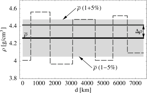
Figure 1: The model of the average matter density as a measured quantity, illustrated for a baseline of $L=7\,500\,\mathrm{km}$ and a matter density uncertainty of $\Delta\rho^{*}=5\%\cdot\bar{\rho}$. The deviation from the average matter density $\bar{\rho}$, i.e., the quantity $\Delta\rho$, is measured by the experiment within the gray-shaded area. This area is determined by $\Delta\rho^{*}=\bar{\rho}\,(1\pm 5\%)$ at the $1\sigma$ confidence level with Gaussian statistics. A possible profile from the random fluctuations model in Ref. [19] is shown as the dashed curve.

In the literature, there exist, in principle, three different classes of models for matter density uncertainties:

Statistical models to study the effects of realistic fluctuations.

These models are averaging over the effects of many profiles with similar properties to be as realistic as possible. Then, the average characteristic effects of matter density uncertainties on the neutrino oscillation transition probabilities or other quantities of interest are studied. Examples are the path integral method to average over many profiles in Refs. [37, 39, 44] and the random fluctuations model in Refs. [19, 41]. In this work, we use the latter one, which demonstrates the dependence on the length scale $\lambda$ and the amplitude $\Delta\rho$ of the fluctuations. In this approach, the actual value of the matter density $\rho$ is fluctuating around the average matter density $\bar{\rho}$ with the length scale $\lambda$ and the amplitude $\Delta\rho$ following some (truncated) Gaussian distributions with standard deviations $\sigma_{\lambda}$ and $\sigma_{\Delta\rho}$, as it is illustrated in Fig. 1 with the dashed curve. From the discrepancies of realistic geophysics profile reconstructions [21], one can estimate a set of standard parameters for these four parameters, which we will use if not otherwise stated: $\lambda\sim 2\,000\,\mathrm{km}$, $\sigma_{\lambda}\sim 3/4\,\lambda$, $\Delta\rho_{0}\sim 3\%\,\bar{\rho}$, and $\sigma_{\Delta\rho}\sim 1/3\,\Delta\rho$.

Simulation models assuming the matter density to be unknown.

The matter density profile is assumed to be unknown within certain limits in order to simulate the matter density uncertainty effects on neutrino oscillation parameter measurements. In these models, the unknown matter density profile (up to a certain degree) implies new parameters to be determined by the measurements, which, of course, are as well correlated amongst themselves as they are correlated with the neutrino oscillation parameters to be measured. Examples include the Fourier expansion method in Refs. [38, 30, 42] and models assuming an uncertainty for the average matter density in Refs. [35, 40, 43, 15, 45]. In Ref. [42], it is shown that the most interesting effects of matter density uncertainties can be translated into an uncertainty (or a shift) of the average matter density along the baseline. In fact, the matter density profile effect can also be incorporated into the model by this approach, where an uncertainty of $5\%$ on the average matter density is quite a safe choice for not too long baselines. The “model of the measured mean matter density”, which is illustrated in Fig. 1, uses the average matter density from the PREM matter density profile and allows it to vary within some range $\Delta\rho^{*}$. It is chosen to be $\Delta\rho^{*}=5\%\cdot\bar{\rho}$ in Refs. [40, 43, 15, 45] using this model in order to safely cover the effects of the matter density uncertainties and even the profile effect for not too long baselines. This means that the average matter density is measured by the experiment within $5\%$ externally imposed precision. From Fig. 1 it should be clear that the random fluctuations can also be simulated with this model, since they are partially averaging out. However, it can be shown that for too large interference effects among the different matter density layers, such as for baselines $L\gtrsim 5\,000\,\mathrm{km}$, the shape of the spectrum changes too much to simply ignore the matter density profile effect. Thus, experiments must, in their data analyses, take into account the profile effects for such long baselines even within this model.

Models for a specific baseline.

For a specific baseline, one can try to obtain further geophysical information in order to incorporate the matter density profile as good as possible (see, for example, Ref. [46]). The deviations from the PREM matter density profile can in this case be rather large. However, the matter density uncertainties of such a profile are drastically reduced.

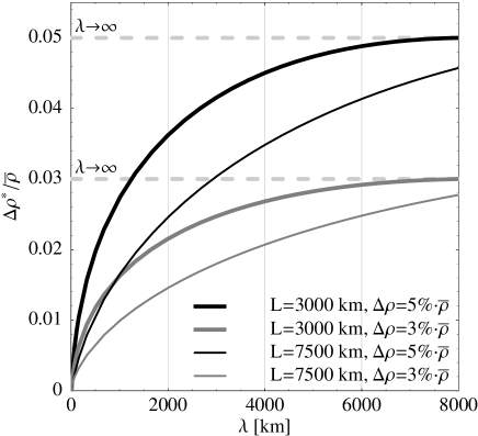
Figure 2: The mapping between the length scale $\lambda$ of the random fluctuations model and the quantity $\Delta\rho^{*}/\bar{\rho}$ of the measured mean model for different fluctuation amplitudes and baselines. For the other parameters from the random fluctuations model in Ref. [19] the standard parameters therein were used: $\sigma_{\lambda}=3/4\,\lambda$ and $\sigma_{\Delta\rho}=1/3\,\Delta\rho$. The mapping is performed by minimizing the $\chi^{2}$-function for the NuFact-II experiment (cf., Sec. 3) between the energy spectrum of a random matter density profile and an average matter density profile with the density $\bar{\rho}+\Delta\rho^{*}$ with respect to the matter density shift $\Delta\rho^{*}$. It turns out that the minimal $\Delta\chi^{2}$ is, for short enough baselines, much smaller than unity, which means that the random matter density profile can be approximated by an average matter density profile to a very good approximation. The shown functions are computed by averaging the shifts $\Delta\rho^{*}$ over $2\,000$ such random profiles and using interpolation.

From the above discussion, it should be obvious that the models within each class are rather similar to each other, although they may be using different approaches and are aiming at different goals. However, one can also transfer knowledge from the statistical models in order to use it for a better estimation of the parameters in the simulation models with unknown matter density parameters. For example, the random fluctuations model (which simulates the effects of the geophysical matter density uncertainties for different length scales and amplitudes to be obtained from geophysics maps) can be used to estimate the precision of the matter density within which it is assumed to be unknown. Let us assume that we can identify the fluctuations to have a certain length scale $\lambda$ and amplitude $\Delta\rho$, what is the deviation of the average matter density $\Delta\rho^{*}$, which needs to be used in the simulations?

As it is noted in Ref. [42], the energy spectrum with the fluctuations can, for short enough baselines, be fit to the one with a constant, but different, average matter density. The average difference between the original and fit average matter densities can then be taken as a measure for the allowed error on the average matter density $\Delta\rho^{*}$. In Fig. 2, this mapping is performed as a function of the length scale $\lambda$ for two different baselines and two different amplitudes of the fluctuations. In this figure, it can clearly be seen that the fluctuations partly average out for short length scales. However, for length scales $\lambda\gg L$ there is no difference between the random fluctuations and the measured average models, since they are identical in this limit. It is also demonstrated that in many cases a somewhat smaller value of $\Delta\rho^{*}$ than $5\%$ should be sufficient for a fluctuation amplitude of $\Delta\rho^{*}=5\%\cdot\bar{\rho}$. However, in this case, the matter density profile effect is not taken into account and it should be kept in mind that we are only comparing average statements.

Closing this argumentation, the different length scales $\lambda$ also correspond to the length scales of certain Fourier modes, which means that fluctuations at a certain length scale leads to an uncertainty of certain Fourier coefficients. These can by their correlation (see Ref. [42]) be translated into an uncertainty of the leading Fourier coefficient. This means that the strength of this correlation between the higher order Fourier coefficients and the leading ones is another qualitative interpretation of Fig. 2. We will therefore further on focus on the effects of the average matter density as a measured quantity in a full statistical analysis, since this should simulate the matter density uncertainties very well and it is suitable for more sophisticated statistical simulations including correlations and degeneracies (cf., Sec. 3).

3 Description of experiment and simulation

Although superbeams are often proposed with quite long baselines, they are either operating in the statistics dominated regime (first-generation experiments) or are limited by the backgrounds and their uncertainties (superbeam upgrades). Therefore, the class of experiments for which matter density uncertainties are most interesting is neutrino factories: First, they usually have long enough baselines, which means that matter effects substantially influence the appearance rates. Second, their precision is very good, which means that matter density uncertainties become a major impact factor. In order to demonstrate the effects of matter density uncertainties, we use the advanced stage neutrino factory setup NuFact-II from Ref. [40] with a muon energy of $50\,\mathrm{GeV}$. This setup has a target power of $4\,\mathrm{MW}$, corresponding to $5.3\cdot 10^{20}$ useful muon decays per year. In addition, we assume eight years of total running time, four of these with a neutrino beam and the other four with an antineutrino beam. For the detector, we simulate a magnetized iron detector with an overall fiducial mass of $50\,\mathrm{kt}$. The baseline length is assumed to be $L=3\,000\,\mathrm{km}$, which has turned out to be reasonable for CP measurements. We use the analysis technique, which is described in the Appendices A, B, and C of Ref. [40], including the beam and detector simulations. As described above, we use the average matter density $\bar{\rho}=3.5\,\mathrm{g/cm^{3}}$, which corresponds to this baseline, and we allow an uncertainty of $\Delta\rho^{*}=5\%\cdot\bar{\rho}$. Later, we will discuss the effect of this uncertainty in greater detail. This means that the matter density is treated as all the other neutrino oscillation parameters to be measured by the neutrino factory. However, the average matter density is assumed to be known from external measurements within some uncertainty, and therefore, the matter density is considered as an external input coming from geophysics (see also Fig. 1). This treatment does not only take into account that the matter density is not precisely known, but it also allows correlations between the neutrino oscillation parameters and the matter density (cf., Ref. [42]). Since we include all relevant appearance and disappearance channels in our analysis, the only parameters which are measured much better with a different class of experiments are the solar parameters. Hence, we use a similar technique to include the external input from the solar parameters and we assume that their product, which the neutrino factories are sensitive to, is measured with $15\%$ precision by the KamLAND experiment by the time the neutrino factory experiment would take place [47, 48].

For the analysis of the quantities of interest we include, where applicable, systematics, multi-parameter correlations, and degeneracies as it is described in Ref. [40] for the individual measurements. To summarize, the treatment of systematics is done in a straightforward way by minimizing the $\chi^{2}$-function over the auxiliary systematic parameters. Multi-parameter correlations are included by projecting the $n$-dimensional fit manifold onto the axis of interest. This approach always needs to be applied if one wants to know the precision of an individual parameter, since the other parameters (such as the CP phase) cannot be determined better by the experiment itself and all possible points within the fit manifold are equally allowed. Alternatively, one could, as a matter of taste, also project onto the plane of two parameters in order to have the information less condensed, but this approach makes it harder to discuss the dependence on the other parameters, such as the true parameter values. As an important difference to the analysis of existing experiments, the reference data set (event rate spectrum) of future experiments is generated with a given set of true parameter values assumed to be realized by Nature and it is not provided by a measurement. In many cases, the results strongly depend on the true parameter values, which can vary within their currently allowed ranges. It is therefore our philosophy to condense the information as much as possible in order to be able to discuss the true parameter value dependencies, which are especially relevant to systematically assess the potential of future experiments.

As far as degeneracies are concerned, we know the $(\delta_{\mathrm{CP}},\theta_{13})$ [35], $\mathrm{sgn}(\Delta m_{31}^{2})$ [49], and $(\theta_{23},\pi/2-\theta_{23})$ [50] degeneracies, which lead to an overall “eight-fold” degeneracy [51]. Since the current best-fit value for the atmospheric mixing angle is $\theta_{23}=\pi/4$, we only consider the first two degeneracies. The definition of the quantity of interest quite often already includes the way the degeneracies have to be treated. For example, defining the sensitivity to $\sin^{2}2\theta_{13}$ as the largest value of $\sin^{2}2\theta_{13}$, which cannot be distinguished from $\sin^{2}2\theta_{13}=0$ (at the chosen confidence level) already implies that any value of $\sin^{2}2\theta_{13}$ fitting $\sin^{2}2\theta_{13}=0$ of any degeneracy is below this sensitivity limit. Thus, for $\sin^{2}2\theta_{13}$ above this sensitivity limit it is guaranteed that we will find $\sin^{2}2\theta_{13}>0$ with the proposed experiment at the chosen confidence level. However, in some cases, including degeneracies is not that straightforward. For example, for the precision of the measurement of $\sin^{2}2\theta_{13}$ we do not find a simple way to include them, and therefore, we only show the results for the best-fit manifold. Similar to the correlations, an existing experiment would analyze its data in a different way. Such as it was performed for a long time with the solar parameters, different isolated islands in the parameter space would be allowed and subsequently reduced by the future experiments (or the combination of some experiments). However, it is the goal of the analyses of future experiments to keep the number (determined by the degeneracies) and the extensions (determined by the correlations) of these islands as small as possible by optimizing the experiments before they are built. Therefore, it is reasonable to condense the information as much as possible in order to discuss the dependencies on the true parameter values.

For the neutrino oscillation parameters, we choose (if not otherwise stated) the best-fit values $\Delta m_{31}^{2}=3.0\cdot 10^{-3}\,\mathrm{eV}^{2}$, $\sin^{2}2\theta_{23}=1.0$ [52], $\Delta m_{21}^{2}=7.0\cdot 10^{-5}\,\mathrm{eV}^{2}$, $\sin^{2}2\theta_{12}=0.8$ (see, for example, Ref. [53]), as well as we only allow values of $\sin^{2}2\theta_{13}$ below the CHOOZ bound and we assume a normal mass hierarchy, i.e., ${\rm sgn}(\Delta m_{31}^{2})=1$. Because of the symmetric operation of the neutrino factory, results would not differ much qualitatively for an inverted mass hierarchy. In general, we do not make any special assumptions about the true value of the CP phase $\delta_{\mathrm{CP}}$. However, in some figures, we will choose certain values for illustrative purposes, since studying the dependence on the CP phase is not the subject of this work.

4 Qualitative discussion of the appearance channels

The goal of this section is to arrive at a qualitative understanding of the effects of matter density uncertainties. However, we will see that there are quite many factors involved in this issue, which we will discuss in the following in somewhat greater detail. At the end of this section, we then will conclude with some very basic qualitative observations.

For long-baseline experiments, the appearance probability $P_{\mathrm{app}}=P_{e\mu}$, $P_{\mu e}$, $P_{\bar{e}\bar{\mu}}$, or $P_{\bar{\mu}\bar{e}}$ in matter can be expanded in the small mass hierarchy parameter $\alpha\equiv\Delta m_{21}^{2}/\Delta m_{31}^{2}$ and the small leptonic mixing angle $\theta_{13}$ up to second order in these parameters as [54, 55, 56]:

$$P_{\mathrm{app}} \equiv P_{1}\pm P_{2}+P_{3}+P_{4}$$ (1)

$$\simeq \sin^{2}2\theta_{13}\,\,\sin^{2}\theta_{23}\,\frac{\sin^{2}[(1-\hat{A}){\hat{\Delta}}]}{(1-\hat{A})^{2}}$$

$$\pm \alpha\,\sin 2\theta_{13}\,\,\sin 2\theta_{12}\,\cos\theta_{13}\,\sin 2\theta_{23}\,\sin\delta_{\mathrm{CP}}\,\sin\hat{\Delta}\,\frac{\sin(\hat{A}{\hat{\Delta}})}{\hat{A}}\,\frac{\sin[(1-\hat{A}){\hat{\Delta}}]}{(1-\hat{A})}$$

$$+ \alpha\,\sin 2\theta_{13}\,\,\sin 2\theta_{12}\,\cos\theta_{13}\,\sin 2\theta_{23}\,\cos\delta_{\mathrm{CP}}\,\cos\hat{\Delta}\,\frac{\sin(\hat{A}{\hat{\Delta}})}{\hat{A}}\,\frac{\sin[(1-\hat{A}){\hat{\Delta}}]}{(1-\hat{A})}$$

$$+ \alpha^{2}\,\,\sin^{2}2\theta_{12}\,\cos^{2}\theta_{23}\,\frac{\sin^{2}(\hat{A}{\hat{\Delta}})}{\hat{A}^{2}}.$$

Here $\hat{\Delta}\equiv\Delta m_{31}^{2}L/(4E)$ and $\hat{A}\equiv\pm(2\sqrt{2}G_{F}n_{e}E)/\Delta m_{31}^{2}$ with $G_{F}$ being the Fermi coupling constant, $L$ the baseline length, $E$ the neutrino energy, and $n_{e}$ the (constant) electron density in matter. This expansion is qualitatively valid independently of the channel used, but the signs before the second term and in the definition of the parameter $\hat{A}$ depend on the direction $\nu_{e}\leftrightarrow\nu_{\mu}$ and if one is using neutrinos or antineutrinos. The sign before the second term is positive for $\nu_{e}\to\nu_{\mu}$ and neutrinos or $\nu_{\mu}\to\nu_{e}$ and antineutrinos and it is negative for $\nu_{e}\to\nu_{\mu}$ and antineutrinos or $\nu_{\mu}\to\nu_{e}$ and neutrinos. The sign in $\hat{A}$ is positive for neutrinos and negative for antineutrinos. Using parameter values for $\alpha$ within the KamLAND-allowed range, it turns out that for long-baseline experiments all four terms in Eq. (1) contribute to the appearance channels with similar orders of magnitude. However, the relative weight of these four terms is determined by the true values of the parameters $\alpha$ and $\theta_{13}$.

In Eq. (1), the matter potential enters via $\hat{A}$ and the matter density resonance condition can be expressed as $\hat{A}\simeq 1$. At the resonance, the factor $\sin[(1-\hat{A})\hat{\Delta}]/(1-\hat{A})$ becomes maximal, which means that the first three terms of Eq. (1) are strongly influenced by the resonance condition. Especially, the quadratic dependency in the first term of Eq. (1) makes it peak much stronger at the resonance than the second and third terms, and therefore suggests that it is most sensitive to a change in any of the parameters in $\hat{A}$. The effect of such a parameter change would also create a shift of the position of the resonance in the neutrino energy spectrum. This is, for example, often used for the sign of $\Delta m_{31}^{2}$-measurement, since $\hat{A}$ changes sign for the inverted mass hierarchy, producing a very distinctive solution. In this case, the resonance is essentially shifted towards negative neutrino energies, which is, of course, an unphysical solution. Since the first term of Eq. (1) is proportional to $\sin^{2}2\theta_{13}$, mass hierarchy measurements are therefore favored for large values of $\sin^{2}2\theta_{13}$ (and small values of $\alpha$ in order to keep the other terms small, which cause correlation and degeneracy problems for this measurement). Another parameter, which enters in $\hat{A}$, is the electron density $n_{e}$ representing the matter density $\rho$. Similar to the sign of $\Delta m_{31}^{2}$, we therefore expect that the neutrino energy spectrum is especially deformed by the first term in Eq. (1) for a shift of the matter density.

In order to demonstrate the above, let us investigate the impact of a perturbation (or shift) $\Delta\hat{A}$ on the parameter $\hat{A}$ somewhat closer. This shift $\Delta\hat{A}$ corresponds to the amplitude of the matter density uncertainty $\Delta\rho$. One can write the absolute shift of the appearance probability $P_{\rm app}$ up to first order in the relative shift of the parameter $\hat{A}$ as:

$$\Delta P_{\rm app} \equiv P_{\rm app}(\hat{A}+\Delta\hat{A})-P_{\rm app}(\hat{A})$$ (2)

$$= \bigg{[}-2\left(\hat{A}\hat{\Delta}\cot[(1-\hat{A})\hat{\Delta}]-\frac{\hat{A}}{1-\hat{A}}\right)P_{1}$$

$$+ \left(-\hat{A}\hat{\Delta}\cot[(1-\hat{A})\hat{\Delta}]+\hat{A}\hat{\Delta}\cot(\hat{A}\hat{\Delta})-\frac{1-2\hat{A}}{1-\hat{A}}\right)P_{2,3}$$

$$+ 2\left(\hat{A}\hat{\Delta}\cot(\hat{A}\hat{\Delta})-1\right)P_{4}\bigg{]}\frac{\Delta\hat{A}}{\hat{A}}+\mathcal{O}\left((\Delta\hat{A}/\hat{A})^{2}\right),$$

where $P_{2,3}\equiv\pm P_{2}+P_{3}$.

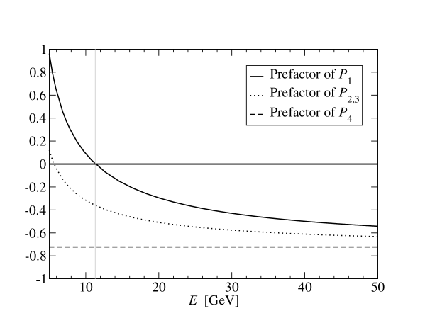
Figure 3: The prefactors of $P_{1}$, $P_{2,3}$, and $P_{4}$ in Eq. (2) as functions of the neutrino energy $E$ ($5\,{\rm GeV}\leq E\leq 50\,{\rm GeV}$) for the parameter values $\Delta m_{31}^{2}=3.0\cdot 10^{-3}\,{\rm eV}^{2}$, $L=3\,000\,{\rm km}$, and $\rho=3.5\,{\rm g/cm^{3}}$. The vertical gray line marks the value of the resonant neutrino energy $E_{\rm res}\simeq 11\,{\rm GeV}$.

The absolute error of the appearance probability $P_{\rm app}$ is here an appropriate representation for the statistical analysis, since the change in the event rates and their impact on the $\chi^{2}$-value is proportional to the absolute (and not relative) error. Note that all prefactors appearing together with the $P_{i}$’s ($i=1,2,3,4$) in Eq. (2) are nearly of the same order of magnitude, at least for neutrino energies $E\gtrsim 20\,\mathrm{GeV}$, as it can be seen from Fig. 3. However, the orders of magnitude of the different terms in Eq. (2) can still be very different from each other, since these terms are proportional to the absolute values of the $P_{i}$’s defined in Eq. (1), which per se could be very different. For example, for large values of $\sin^{2}2\theta_{13}$ the first term in Eq. (1) is relatively large and would therefore also be strongly affected by matter density uncertainties. In addition, all terms in Eq. (2) are proportional to $\Delta\hat{A}/\hat{A}$ to first order, which means that the absolute change of one of the terms is obtained by multiplying the prefactor with the relative change of the matter density and the corresponding $P_{i}$ itself. In Fig. 3, we observe that all prefactors are finite and not singular at the resonant neutrino energy $E_{\rm res}\simeq 11\,{\rm GeV}$ and that the prefactor of $P_{4}$ is a constant with respect to the neutrino energy $E$. Most interesting, the prefactor of $P_{1}$ changes sign at the resonance, which means that a small shift $\Delta\hat{A}$ of the matter density close to the resonance will cause

• a spectral distortion and a change of the normalization in the first (and also somewhat in the second and third) term

• only a change of the normalization in the fourth term

of Eq. (1). Since the effects of the matter density shift can be of equal size, this observation makes the analysis of matter density uncertainties rather complicated. However, it should be noted that especially the first term can also simulate spectral distortion effects in addition to a change of the normalization, which means that it allows more sophisticated correlations than the other terms.

As far as correlations are concerned, we observe that in Eq. (1) only the combinations

$$C_{1} = \sin 2\theta_{13}\,\frac{\sin[(1-\hat{A})\hat{\Delta}]}{1-\hat{A}},$$ (3)

$$C_{2} = \alpha\,\sin 2\theta_{12}\,\frac{\sin(\hat{A}{\hat{\Delta}})}{\hat{A}}$$ (4)

are present. In Eq. (1), $C_{1}^{2}$ appears in the first term, $C_{1}C_{2}$ in the second and third terms, and $C_{2}^{2}$ in the fourth term. This means that a change in any parameter value in these terms can be compensated by another one. Since $\sin^{2}2\theta_{13}$ is the quantity of interest to us, it will lead to correlations with the matter density shift $\Delta\hat{A}$. However, the quantities $\alpha$ and $\sin 2\theta_{12}$ are given by external measurements with lower precisions than the matter density, which means that they can easily absorb a change of the matter density from the correlation in the first term of Eq. (1). Therefore, especially for large $\sin^{2}2\theta_{13}$, where the influence of matter density uncertainties to the first term in Eq. (1) is large (cf., Eq. (2)), the combination $C_{1}$ can have a major impact on measurements.

Another important ingredient in the analysis is statistics. This means that the impact of the matter density uncertainties can be suppressed in statistics dominated regions of the parameter space. Since some measurements are limited by statistics, the matter density uncertainty will not at all have a strong impact on these measurements. For example, the $\sin^{2}2\theta_{13}$-sensitivity limit describes the ability for an experiment to establish $\sin^{2}2\theta_{13}>0$. In this case, the reference rate vector is computed with $\sin^{2}2\theta_{13}=0$ and the statistics from the first three terms in Eq. (1), which are only present for $\sin^{2}2\theta_{13}>0$, limits the measurement. Thus, the $\sin^{2}2\theta_{13}$-sensitivity limit is constrained by the absolute size of these terms, which cannot be compensated by the correlation with matter density uncertainties because of the spectral dependence of the first prefactor in Eq. (2). Since all of the quantities of interest to us are suppressed by $\sin 2\theta_{13}$ in Eq. (1), a similar argument can be used for small values of $\sin^{2}2\theta_{13}$, where most measurements are limited by the statistics in the appearance channels and not by the matter density uncertainties. In addition, matter density uncertainties will turn out not to be relevant for many measurements with a strong “binary nature”, i.e., measurements which only have two very distinctive different answers. The ability to distinguish these two answers often depends more on statistics than on the matter density uncertainty, which cannot simulate the different solution. One such example is the mass hierarchy determination discussed above, which could only be mimicked by matter density uncertainties larger than $100\%\cdot\bar{\rho}$.

Putting all pieces together, we have found that especially $\sin^{2}2\theta_{13}$ as a quantity of interest is highly correlated with the matter density uncertainties. However, the effects of the matter density uncertainties are proportional to the four terms in Eq. (1) themselves, which means that they are (for the quantities of interest) suppressed by $\sin^{2}2\theta_{13}$ itself. Therefore, we expect a large influence of matter density uncertainties for large $\sin^{2}2\theta_{13}$ and a small influence for small $\sin^{2}2\theta_{13}$ because of domination of statistics. For the $\sin^{2}2\theta_{13}$-precision measurement the correlation between $\sin^{2}2\theta_{13}$ and the matter density uncertainties should be limiting the measurements for large values of $\sin^{2}2\theta_{13}$. However, for CP measurements the first term in Eq. (1) acts as a background. The matter density uncertainties should introduce an additional systematical error for large values of $\sin^{2}2\theta_{13}$, such as a background uncertainty. In addition, $\delta_{\mathrm{CP}}$ is highly correlated with $\sin^{2}2\theta_{13}$, which again is correlated with $\Delta\hat{A}$, which suggests that it is also indirectly affected via this correlations. However, since the relative impact of the first term in Eq. (1) decreases for increasing $\alpha$, also the effects of the matter density uncertainties should become smaller.

5 The results for the different measurements

In this section, we systematically discuss the impact of matter density uncertainties on the most interesting measurements at a neutrino factory: $\sin^{2}2\theta_{13}$, the sign of $\Delta m_{31}^{2}$, and $\delta_{\mathrm{CP}}$. Although many of these measurements have been individually treated in previous works, the goal of this work is to specifically demonstrate where in parameter space and for which measurements matter density uncertainties are relevant and important. In addition, we will show, where applicable, representative examples of such measurements as functions of the amplitude of the matter density uncertainties. We choose the “model of the measured mean matter density” with the values $\Delta\rho^{*}=0$ (no matter density uncertainties), $\Delta\rho^{*}=1\%\cdot\bar{\rho}$, $\Delta\rho^{*}=3\%\cdot\bar{\rho}$, $\Delta\rho^{*}=5\%\cdot\bar{\rho}$ (the standard value, which we usually propose as a conservative choice), and $\Delta\rho^{*}=10\%\cdot\bar{\rho}$ (the most pessimistic choice).

The sensitivity to $\sin^{2}2\theta_{13}$

We define the sensitivity to $\sin^{2}2\theta_{13}$ as the largest value of $\sin^{2}2\theta_{13}$, which fits the true value $\sin^{2}2\theta_{13}=0$. As discussed in the previous section, this choice naturally includes the treatment of correlations and degeneracies, which means that any point in the multi-dimensional parameter space, which fits the zero rate vector at the chosen confidence level, will have a fit value of $\sin^{2}2\theta_{13}$ below the sensitivity limit. Thus, it is guaranteed that the experiment will find $\sin^{2}2\theta_{13}$ above the sensitivity limit at the chosen confidence level. Any other definition of the sensitivity limit would be more complicated and would involve a more sophisticated definition of how to treat degeneracies. For example, one could show the sensitive ranges for the different degeneracies separately. Such a definition might be sensible for existing experiments, but not to evaluate and compare the potential of future experiments in order to optimize them using condensed information.

As we qualitatively discussed in Sec. 4, the sensitivity to $\sin^{2}2\theta_{13}$ is limited by the statistics in the appearance channels. Therefore, the systematics introduced by the matter density uncertainties does not affect it substantially. This can, for example, be seen from comparing Fig. 9 with Fig. 10 in Ref. [40] for NuFact-II. In this impact factor analysis, the matter density affects the $\sin^{2}2\theta_{13}$-precision measurements, but it does not at all affect the $\sin^{2}2\theta_{13}$-sensitivity limit.

The precision of $\sin^{2}2\theta_{13}$

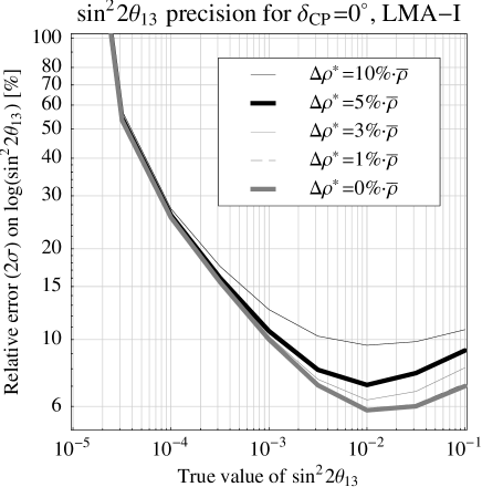
Figure 4: The precision of the measurement of $\sin^{2}2\theta_{13}$ (full width, best-fit manifold only) for NuFact-II and the true value of $\delta_{\mathrm{CP}}=0$ as a function of the true value of $\sin^{2}2\theta_{13}$ at the $2\sigma$ confidence level. The different curves correspond to different allowed matter density uncertainties $\Delta\rho^{*}$ as described in the plot legend, especially the thick curves correspond to no matter density uncertainty (light thick curve) and our standard uncertainty $\Delta\rho^{*}=5\%\cdot\bar{\rho}$ (dark thick curve).

We define the precision of $\sin^{2}2\theta_{13}$ as the full width error (at the chosen confidence level) of the best-fit manifold projected onto the $\sin^{2}2\theta_{13}$-axis. This definition includes correlations, but it does not include (disconnected) degeneracies, since a sensible definition of the $\sin^{2}2\theta_{13}$-precision including disconnected degeneracies is difficult. In Fig. 4, we show the relative error on $\mathrm{log}(\sin^{2}2\theta_{13})$ on a double-logarithmic scale. In addition, we only show it for one true value of $\delta_{\mathrm{CP}}=0$, since otherwise one could not clearly see the effect of the matter density uncertainty. However, one should keep in mind that this precision strongly depends on the true value of $\delta_{\mathrm{CP}}$. A possible representation of this fact is to show the band ranging over all true values of the CP phase, such as it is done in Fig. 13 of Ref. [40].

Figure 4 demonstrates the effects of the matter densities as a function of their amplitude $\Delta\rho^{*}$ for the LMA-I solution, where the dark thick curve corresponds to our standard choice and the light thick curve to no matter density uncertainties, which is often used in other studies. Except from the most extreme (and unrealistic) case of $\Delta\rho^{*}=10\%\cdot\bar{\rho}$, we do not find any significant influence of the matter density uncertainties below $\sin^{2}2\theta_{13}\lesssim 10^{-3}$. In this region, the $\sin^{2}2\theta_{13}$-dependent terms in Eq. (1) are more determined by the statistics than the matter density uncertainty. However, at the CHOOZ limit, the matter density uncertainties lead to corrections at the percent level of the investigated quantity. It is also interesting to note that for $\Delta\rho^{*}\lesssim 1\%\cdot\bar{\rho}$ the matter density uncertainties are irrelevant. Figure 4 is representative for different values of $\delta_{\mathrm{CP}}$ than $\delta_{\mathrm{CP}}=0^{\circ}$. For example, if one drew bands using all values of $\delta_{\mathrm{CP}}$ (such as in Fig. 13 of Ref. [40]), the matter density uncertainties would lead to an upward shift of these bands for large values of $\sin^{2}2\theta_{13}$. A similar qualitative behavior can also be expected for the LMA-II solution, although the general performance with respect to $\sin^{2}2\theta_{13}$ is worse because of the stronger presence of correlations and degeneracies.

The sensitivity to the sign of $\Delta m_{31}^{2}$

We define that there is a sensitivity to a certain sign of $\Delta m_{31}^{2}$, if there is no solution fitting the zero rate vector (generated with this specific sign) with the opposite sign of $\Delta m_{31}^{2}$ at the chosen confidence level. This definition implies that the presence of the $\mathrm{sgn}(\Delta m_{31}^{2})$-degeneracy at the chosen confidence level is the most important factor, which destroys the sign of the $\Delta m_{31}^{2}$-sensitivity. Performing the analysis, it turns out that the matter density uncertainty hardly affects the appearance of the degenerate solution. This means that matter density uncertainties are not relevant for the sign of the $\Delta m_{31}^{2}$-determination, at least within the KamLAND-allowed range, even $\Delta\rho^{*}=10\%\cdot\bar{\rho}$ is safe for NuFact-II. Given the definition of $\hat{A}$ at Eq. (1), a compensation of a different sign of $\Delta m_{31}^{2}$ in $\hat{A}$ could only be achieved by reversing the sign of $\rho$, i.e., negative matter densities. However, in our analysis, such a reversion would require matter density uncertainties of over $100\%\cdot\bar{\rho}$ in order to allow the unphysical assumption of antimatter in the Earth.

The sensitivity to any CP violation

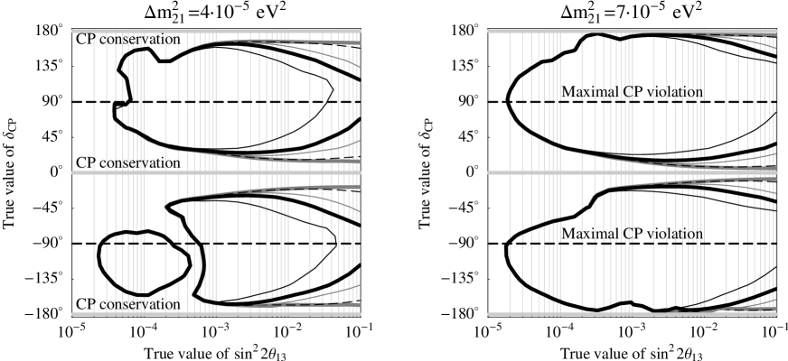
Figure 5: The sensitivity to CP violation for NuFact-II and two different values of $\Delta m_{21}^{2}$ as a function of the true values of $\sin^{2}2\theta_{13}$ and $\delta_{\mathrm{CP}}$ at the $2\sigma$ confidence level. The parameter values within the regions enclosed by the contours refer to the sensitivity to CP violation, i.e., the ability to distinguish the respective true value of $\delta_{\mathrm{CP}}$ given at the vertical axis from $\delta_{\mathrm{CP}}\in\{0,180^{\circ}\}$ (CP conservation). The different curves correspond to different values of $\Delta\rho^{*}$ as given in the legend of Fig. 4, especially the thick curves correspond to no matter density uncertainty (light thick curve) and our standard uncertainty $\Delta\rho^{*}=5\%\cdot\bar{\rho}$ (dark thick curve).

One can define the sensitivity to any CP violation as the ability of an experiment to distinguish any given true CP violating value $\delta_{\mathrm{CP}}\notin\{0,180^{\circ}\}$ from the CP conserving values $\delta_{\mathrm{CP}}\in\{0,180^{\circ}\}$. This definition already implies the treatment of degeneracies: any degenerate solution fitting $\delta_{\mathrm{CP}}\in\{0,180^{\circ}\}$ would destroy the sensitivity to CP violation. A special case of CP violation covered by this definition is the case of maximal CP violation with the true value $\delta_{\mathrm{CP}}\in\{-90^{\circ},90^{\circ}\}$, which we will discuss in the next subsection.

Figure 5 shows the sensitivity to any CP violation as a function of the true values of $\sin^{2}2\theta_{13}$ and $\delta_{\mathrm{CP}}$ for several different values of the matter density uncertainty. The left-hand side plot corresponds to the current lower limit of the KamLAND-allowed range, whereas the right-hand side plot corresponds to the LMA-I best-fit value. Again, the matter density uncertainties are only relevant for $\sin^{2}2\theta_{13}\gtrsim 10^{-3}$, as it can be clearly seen in Fig. 5, and the measurements are statistics dominated for $\sin^{2}2\theta_{13}\lesssim 10^{-3}$. Comparing the dark thick curves for our standard value $\Delta\rho^{*}=5\%\cdot\bar{\rho}$ between the left- and right-hand side plots at the CHOOZ limit indicates that the relative influence of the matter density uncertainties decreases with increasing $\Delta m_{21}^{2}$. In general, the CP performance becomes better for a large hierarchy parameter $\alpha\equiv\Delta m_{21}^{2}/\Delta m_{31}^{2}$ in Eq. (1), where the CP sensitive terms also become large. Thus, the relative impact from the matter density uncertainties in the first term of Eq. (1) decreases for larger values of $\alpha$. In addition, problems with degeneracies are reduced by better statistics of the CP sensitive terms. Another important conclusion from Fig. 5 is that for $\Delta\rho^{*}\lesssim 1\%\cdot\bar{\rho}$ the matter density uncertainties are again not relevant.

The sensitivity to maximal CP violation

The special case of sensitivity to maximal CP violation $\delta_{\mathrm{CP}}\in\{-90^{\circ},90^{\circ}\}$ is represented by the horizontal dashed lines in Fig. 5. This measurement has a much more “binary nature” than the sensitivity to a small CP violation, since CP conservation and maximal CP violation produce rather distinctive rate vectors for large values of $\sin^{2}2\theta_{13}$, where matter density uncertainties are most important. Since the sensitivity to maximal CP violation is close to the optimum of all CP violation sensitivities, it is often used as a representative for CP violation discussions. For example, it is shown as a function of the true values of $\sin^{2}2\theta_{13}$ and $\Delta m_{21}^{2}$ in Fig. 17 of Ref. [40], a presentation, which would not be possible for any CP violation.

It can be shown that matter density uncertainties are not important for maximal CP violation measurements at the $2\sigma$ confidence level within the ($3\sigma$) KamLAND-allowed range as long as $\Delta\rho^{*}\lesssim 5\%\cdot\bar{\rho}$. This is consistent with Fig. 5 along the horizontal dashed lines, since the left-hand side plot represents the lower limit of the KamLAND-allowed range and the relative influence of the matter density uncertainties becomes smaller for larger values of $\Delta m_{21}^{2}$. Only for very large matter density uncertainties $\Delta\rho^{*}=10\%\cdot\bar{\rho}$, they have some impact on the very lower end of the KamLAND-allowed range. However, note that this statement does not mean that matter density uncertainties in general do not affect the (maximal) CP violation measurements. It depends on the used parameter values and it is supported by the fact that the KamLAND experiment cut off the lower part of the LMA solution.

The precision of $\delta_{\mathrm{CP}}$

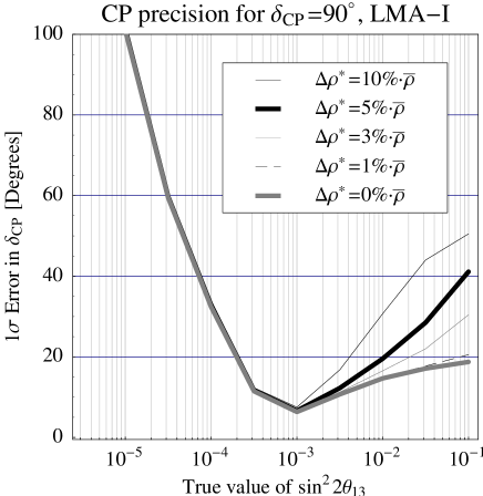
Figure 6: The precision of the measurement of $\delta_{\mathrm{CP}}$ (full width) for NuFact-II and the true value of $\delta_{\mathrm{CP}}=90^{\circ}$ as a function of the true value of $\sin^{2}2\theta_{13}$ at the $1\sigma$ confidence level. The different curves correspond to different allowed matter density uncertainties $\Delta\rho^{*}$ as described in the plot legend, especially the thick curves correspond to no matter density uncertainty (light thick curve) and our standard uncertainty $\Delta\rho^{*}=5\%\cdot\bar{\rho}$ (dark thick curve).

We define the precision of $\delta_{\mathrm{CP}}$ as the full width error of $\delta_{\mathrm{CP}}$ on the “CP circle”. For a given true value of $\delta_{\mathrm{CP}}$ any degenerate solution, which fits the true value, is included in this precision. It is sometimes also called the “coverage in $\delta_{\mathrm{CP}}$” [40], because it describes how much of the CP circle that fits the chosen true value of $\delta_{\mathrm{CP}}$. Thus, a precision of $360^{\circ}$ (or a coverage of $100\%$) corresponds to no improvement of the knowledge on $\delta_{\mathrm{CP}}$. In comparison to the CP violation sensitivity, the precision of $\delta_{\mathrm{CP}}$ does not differentiate any special value of $\delta_{\mathrm{CP}}$, such as the CP conserving values $0$ and $180^{\circ}$. It describes how much one could learn about $\delta_{\mathrm{CP}}$ from a specific experiment. For example, even if an experiment is not sensitive to CP violation, because $\delta_{\mathrm{CP}}$ is too close to CP conservation, it may teach us something about $\delta_{\mathrm{CP}}$ and exclude certain regions of the CP circle. In this case, the precision (coverage) would be smaller than $360^{\circ}$.

In Fig. 6, the precision of $\delta_{\mathrm{CP}}$ is shown as a function of the true value of $\sin^{2}2\theta_{13}$ for the true value $\delta_{\mathrm{CP}}=90^{\circ}$ at the $1\sigma$ confidence level. One could also choose a different true value of $\delta_{\mathrm{CP}}$ or a different confidence level, but the effects of the matter density uncertainties would qualitatively look the same. However, degeneracies are hardly present below the $1\sigma$ confidence level. Therefore, the numbers on the precision axis should be handled with care, since the $3\sigma$ errors would be over-proportionally larger not following simple Gaussian statistics. As for the case of CP violation, matter density uncertainties become important for $\sin^{2}2\theta_{13}\gtrsim 10^{-3}$ and $\Delta\rho^{*}>1\%\cdot\bar{\rho}$ for the same reasons. However, since the CP precision measurement includes all possible fit values of $\delta_{\mathrm{CP}}$ and it is not a binary measurement, the effects of the matter density uncertainties can be very large. At the CHOOZ limit, they can even affect the precision by a factor of two or more.

6 Summary and conclusions

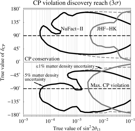
Figure 7: The $3\sigma$ CP violation discovery reach as a function of the true values of $\sin^{2}2\theta_{13}$ and $\delta_{\mathrm{CP}}$ for NuFact-II and JHF-HK from Ref. [40]. The parameter values within the regions enclosed by the contours correspond to the sensitivity to CP violation, i.e., the ability to distinguish the respective true value of $\delta_{\mathrm{CP}}$ given at the vertical axis from $\delta_{\mathrm{CP}}\in\{0,180^{\circ}\}$, i.e., CP conservation. The different curves correspond to different values of $\Delta\rho^{*}$ as given in the figure. For the JHF-HK experiment, matter effects (and matter density uncertainty effects) are strongly suppressed by the short baseline $L\simeq 295\,\mathrm{km}$. For the NuFact-II experiment, degeneracies are much more present at the $3\sigma$ confidence level than at the $2\sigma$ confidence level, as it can be seen by comparison with Fig. 5 (right-hand side plot).

Matter density uncertainties up to $5\%$ can be present on the PREM matter density profile. It is well known that they can influence many of the measurements at a future neutrino factory, such as the CP precision measurements. In this work, we have first of all discussed different approaches to model the matter density uncertainties and how they are related to each other. We have concluded that using the average matter density with an uncertainty of about $\Delta\rho^{*}=3\%$ - $5\%$ is an appropriate conservative choice for a complete statistical neutrino factory simulation. In this approach, the average matter density is measured by the neutrino factory as an independent parameter within the externally given precision $\Delta\rho^{*}$. It has several advantages:

• It is fast enough for a complete statistical simulation including systematics, correlations, and degeneracies.

• It allows correlations between the matter density and the neutrino oscillation parameters.

• It can use the external information from other statistical models or a specific baseline to improve the knowledge on the input parameter $\Delta\rho^{*}$.

• It can even simulate the matter density profile effect for not too long baselines ($L\lesssim 5\,000\,\mathrm{km}$).

With this model, we have systematically discussed how the matter density uncertainties affect the most important measurements at a large neutrino factory at a baseline of $L=3\,000\,\mathrm{km}$. We have found that some, but not all, measurements suffer from the matter density uncertainties. In addition, they are only relevant in certain regions of the parameter space. In detail, we have found that

For the $\sin^{2}2\theta_{13}$-sensitivity

matter density uncertainties are not important, because this measurement is constrained by the statistics in the appearance channels and not by the systematics coming from the matter density uncertainties.

For the $\sin^{2}2\theta_{13}$-precision

matter density uncertainties are only relevant for $\sin^{2}2\theta_{13}\gtrsim 10^{-3}$ because of the statistics domination below that region.

For the sign of $\Delta m_{31}^{2}$-sensitivity

matter density uncertainties are irrelevant because of the very distinctive solutions of this binary measurement, which could only be mixed up by the matter density uncertainties by using negative matter densities.

For the sensitivity to any CP violation

matter density uncertainties again become important for $\sin^{2}2\theta_{13}\gtrsim 10^{-3}$. However, their relative influence is reduced for large values of $\Delta m_{21}^{2}$.

For the sensitivity to maximal CP violation

matter density uncertainties are not significantly important within the KamLAND-allowed range at the $2\sigma$ confidence level.

For the precision of $\delta_{\mathrm{CP}}$

matter density uncertainties are not important for $\sin^{2}2\theta_{13}\lesssim 10^{-3}$. However, for $\sin^{2}2\theta_{13}\gtrsim 10^{-3}$ they make the precision worse by a factor of two (close to the CHOOZ limit).

We conclude that three conditions are necessary for the matter density uncertainties to become relevant at the considered neutrino factory analysis: First, only some of the measurements are influenced by matter density uncertainties, such as the $\sin^{2}2\theta_{13}$- and $\delta_{\mathrm{CP}}$-precision measurements. Second, matter density uncertainties are only important for $\sin^{2}2\theta_{13}\gtrsim 10^{-3}$. Third, matter density uncertainties only sensibly affect the measurements for uncertainty amplitudes $\Delta\rho^{*}\gtrsim 1\%\cdot\bar{\rho}$, as it can be observed in any of the figures so far.

Since superbeams or superbeam upgrades are basically sensitive down to $\sin^{2}2\theta_{13}\sim 10^{-3}$ for the discussed measurements, competitiveness of neutrino factories with superbeams is an interesting issue. Superbeams are often proposed with shorter baselines and they are using different (non-resonant) neutrino energies, which means that they are much less affected by matter density uncertainties. This is one of the reasons why they are often much better than the neutrino factories for $\sin^{2}2\theta_{13}\gtrsim 10^{-3}$. For illustration, the $3\sigma$ CP violation discovery potential is shown in Fig. 7 for NuFact-II (with $\Delta\rho^{*}=5\%\cdot\bar{\rho}$ and $\Delta\rho^{*}\lesssim 1\%\cdot\bar{\rho}$) and the JHF to Hyper-Kamiokande superbeam upgrade JHF-HK from Ref. [40] (as it is proposed in Ref. [11], using two years of neutrino running and six years of antineutrino running). Since this superbeam upgrade is proposed with a quite short baseline $L\simeq 295\,\mathrm{km}$, it is hardly affected by matter effects and matter density uncertainty effects. The figure clearly demonstrates that especially for $\sin^{2}2\theta_{13}\gtrsim 10^{-2}$ a knowledge on the matter density profile with about $1\%$ precision is necessary for the competitiveness of neutrino factories with superbeams. Therefore, it would be interesting to know with what costs such a precision could be achieved in geophysics along a specific baseline. However, if the superbeams do not find $\sin^{2}2\theta_{13}>0$, then the neutrino factories will for $\sin^{2}2\theta_{13}\lesssim 10^{-3}$ be almost unaffected by matter density uncertainties in the post-superbeam era.

Acknowledgments

We would like to thank Steve Geer, Patrick Huber, and Manfred Lindner for useful discussions and comments. T.O. and W.W. would like to thank TUM and KTH-SCFAB, respectively, for the warm hospitality during their respective visits at the other university. This work was supported by the Magnus Bergvall Foundation (Magn. Bergvalls Stiftelse), the ESF Network on Neutrino Astrophysics [T.O.], the Swedish Research Council (Vetenskapsrådet), Contract No. 621-2001-1611, 621-2002-3577 [T.O.], the Göran Gustafsson Foundation (Göran Gustafssons Stiftelse) [T.O.], the “Studienstiftung des deutschen Volkes” (German National Merit Foundation) [W.W.], and the “Sonderforschungsbereich 375 für Astro-Teilchenphysik der Deutschen Forschungsgemeinschaft” [W.W.].

References

- [1] Super-Kamiokande Collaboration, Y. Fukuda et al., Phys. Rev. Lett. 81 (1998) 1562, hep-ex/9807003.
- [2] Super-Kamiokande Collaboration, Y. Fukuda et al., Phys. Rev. Lett. 82 (1999) 2644, hep-ex/9812014.
- [3] SNO Collaboration, Q.R. Ahmad et al., Phys. Rev. Lett. 87 (2001) 071301, nucl-ex/0106015.
- [4] SNO Collaboration, Q.R. Ahmad et al., Phys. Rev. Lett. 89 (2002) 011301, nucl-ex/0204008.
- [5] KamLAND Collaboration, K. Eguchi et al., Phys. Rev. Lett. 90 (2003) 021802, hep-ex/0212021.
- [6] CHOOZ Collaboration, M. Apollonio et al., Phys. Lett. B466 (1999) 415, hep-ex/9907037.
- [7] CHOOZ Collaboration, M. Apollonio et al., Eur. Phys. J. C27 (2003) 331, hep-ex/0301017.
- [8] K2K Collaboration, K. Nakamura, Nucl. Phys. Proc. Suppl. 91 (2001) 203.
- [9] MINOS Collaboration, V. Paolone, Nucl. Phys. Proc. Suppl. 100 (2001) 197.
- [10] A. Ereditato, Nucl. Phys. Proc. Suppl. 100 (2001) 200.
- [11] Y. Itow et al., Nucl. Phys. Proc. Suppl. 111 (2001) 146, hep-ex/0106019.
- [12] D. Ayres et al., hep-ex/0210005.
- [13] D. Beavis et al., hep-ex/0205040.
- [14] M. Apollonio et al., hep-ph/0210192, and references therein.
- [15] P. Huber and W. Winter, Phys. Rev. D (to be published), hep-ph/0301257.
- [16] L. Wolfenstein, Phys. Rev. D17 (1978) 2369.
- [17] S.P. Mikheev and A.Y. Smirnov, Sov. J. Nucl. Phys. 42 (1985) 913, [Yad. Fiz. 42 (1985) 1441].
- [18] S.P. Mikheev and A.Y. Smirnov, Nuovo Cim. C9 (1986) 17.
- [19] B. Jacobsson et al., Phys. Lett. B532 (2002) 259, hep-ph/0112138.
- [20] A.M. Dziewonski and D.L. Anderson, Phys. Earth Planet. Interiors 25 (1981) 297.
-
[21]
S.V. Panasyuk,
REM (Reference Earth Model) web page,
http://cfauvcs5.harvard.edu/lana/rem/index.htm - [22] R.J. Geller and T. Hara, Nucl. Instrum. Meth. A503 (2001) 187, hep-ph/0111342.
- [23] J. Arafune, M. Koike and J. Sato, Phys. Rev. D56 (1997) 3093, hep-ph/9703351.
- [24] H. Minakata and H. Nunokawa, Phys. Rev. D57 (1998) 4403, hep-ph/9705208.
- [25] P. Lipari, Phys. Rev. D61 (2000) 113004, hep-ph/9903481.
- [26] M. Narayan and S. Uma Sankar, Phys. Rev. D61 (2000) 013003, hep-ph/9904302.
- [27] M. Freund et al., Nucl. Phys. B578 (2000) 27, hep-ph/9912457.
- [28] M. Campanelli, A. Bueno and A. Rubbia, Nucl. Instrum. Meth. A451 (2000) 207.
- [29] I. Mocioiu and R. Shrock, Phys. Rev. D62 (2000) 053017, hep-ph/0002149.
- [30] T. Ota and J. Sato, Phys. Rev. D63 (2001) 093004, hep-ph/0011234.
- [31] M. Freund, P. Huber and M. Lindner, Nucl. Phys. B585 (2000) 105, hep-ph/0004085.
- [32] T. Miura et al., Phys. Rev. D64 (2001) 013002, hep-ph/0102111.
- [33] B. Brahmachari, S. Choubey and P. Roy, hep-ph/0303078.
- [34] M. Koike and J. Sato, Mod. Phys. Lett. A14 (1999) 1297, hep-ph/9803212.
- [35] J. Burguet-Castell et al., Nucl. Phys. B608 (2001) 301, hep-ph/0103258.
- [36] T. Miura et al., Phys. Rev. D64 (2001) 073017, hep-ph/0106086.
- [37] L.Y. Shan, B.L. Young and X.m. Zhang, Phys. Rev. D66 (2002) 053012, hep-ph/0110414.
- [38] G.L. Fogli, G. Lettera and E. Lisi, hep-ph/0112241.
- [39] L.Y. Shan and X.M. Zhang, Phys. Rev. D65 (2002) 113011.
- [40] P. Huber, M. Lindner and W. Winter, Nucl. Phys. B645 (2002) 3, hep-ph/0204352.
- [41] B. Jacobsson et al., J. Phys. G29 (2003) 1873, hep-ph/0209147.
- [42] T. Ota and J. Sato, Phys. Rev. D67 (2003) 053003, hep-ph/0211095.
- [43] P. Huber, M. Lindner and W. Winter, Nucl. Phys. B654 (2003) 3, hep-ph/0211300.
- [44] L.Y. Shan et al., Phys. Rev. D68 (2003) 013002, hep-ph/0303112.
- [45] P. Huber et al., Nucl. Phys. B (to be published), hep-ph/0303232.
- [46] E. Kozlovskaya, J. Peltoniemi and J. Sarkamo, hep-ph/0305042.
-
[47]
V. Barger, D. Marfatia and B. Wood,
Phys. Lett. B498 (2001) 53,
hep-ph/0011251. - [48] M.C. Gonzalez-Garcia and C. Pea-Garay, Phys. Lett. B527 (2002) 199, hep-ph/0111432.
- [49] H. Minakata and H. Nunokawa, J. High Energy Phys. 10 (2001) 001, hep-ph/0108085.
- [50] G.L. Fogli and E. Lisi, Phys. Rev. D54 (1996) 3667, hep-ph/9604415.
- [51] V. Barger, D. Marfatia and K. Whisnant, Phys. Rev. D65 (2002) 073023, hep-ph/0112119.
- [52] M.C. Gonzalez-Garcia and M. Maltoni, Eur. Phys. J. C26 (2003) 417, hep-ph/0202218.
- [53] M. Maltoni, T. Schwetz and J.W.F. Valle, Phys. Rev. D67 (2003) 093003, hep-ph/0212129.
- [54] A. Cervera et al., Nucl. Phys. B579 (2000) 17, hep-ph/0002108, B593 (2001) 731(E).
- [55] M. Freund, P. Huber and M. Lindner, Nucl. Phys. B585 (2000) 105, hep-ph/0004085.
- [56] M. Freund, Phys. Rev. D64 (2001) 053003, hep-ph/0103300.