On the analysis of the $\pi\to e\nu\gamma$ experimental data

Abstract

The most general amplitude for the radiative pion decay $\pi\to e\nu\gamma$ including terms beyond V-A theory is considered. The experimental constraints on the decay amplitude components are discussed. A model independent presentation of the results of high statistics and high resolution experiments is suggested.

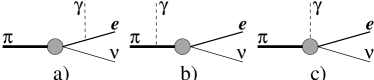
Figure 1: The $\pi\to e\nu\gamma$ diagrams

Due to the strong helicity suppression of the $\pi\to e\nu$ decay, the corresponding radiative decay

$$\pi\to e\nu\gamma$$ (1)

is regarded as a valuable source of pion structure information and a sensitive test anomalous interactions Bardin and Ivanov (1976); Bryman et al. (1982). Low’s theorem Low (1958) allows the part of the $\pi\to e\nu\gamma$ amplitude depending on the photon energy $\omega$ as $\omega^{-1}$ and $\omega^{0}$ to be unambiguously defined by the pion decay constant $f_{\pi}=131~{}\mathrm{MeV}$. This contribution to the decay amplitude, called inner bremsstrahlung ($IB$), is associated with the tree diagrams shown in Figs. 1a) and 1b). Generally, one can construct the remaining, structure dependent ($SD$) part of the amplitude (Fig. 1c)) using the photon tensors ${\cal F}^{\mu\nu}_{\pm}=k^{\mu}\epsilon^{\nu}-k^{\nu}\epsilon^{\mu}\pm ie^{\mu\nu\alpha\beta}k^{\alpha}\epsilon^{\beta}$ where $\epsilon^{\mu}$ is the photon polarization vector and $\pm$ specify the photon helicities, the lepton currents $L=\bar{u}_{\nu}(1+\gamma^{5})u_{e}$, $L^{\mu}=\bar{u}_{\nu}(1+\gamma^{5})\gamma^{\mu}u_{e}$, $L^{\mu\nu}=\bar{u}_{\nu}(1+\gamma^{5})\sigma^{\mu\nu}u_{e}$, and three available 4-momenta $k^{\mu}$, $q^{\mu}=l^{\mu}+t^{\mu}$, and $r^{\mu}=l^{\mu}-t^{\mu}$, where $k^{\mu}$, $l^{\mu}$, and $t^{\mu}$ are 4-momenta of photon, electron, and neutrino, respectively. Using the Dirac equation and properties of $\gamma$-matrices the full list of such amplitudes: ${\cal F}^{\mu\nu}_{\pm}a^{\mu}b^{\nu}L$, ${\cal F}^{\mu\nu}_{\pm}a^{\mu}b^{\nu}L^{\rho}c^{\rho}$, ${\cal F}^{\mu\nu}_{\pm}a^{\mu}b^{\nu}L^{\rho\sigma}c^{\rho}d^{\sigma}$, ${\cal F}^{\mu\nu}_{\pm}a^{\mu}L^{\nu}$, ${\cal F}^{\mu\nu}_{\pm}a^{\mu}b^{\rho}L^{\nu\rho}$, and ${\cal F}^{\mu\nu}_{\pm}L^{\mu\nu}$, may be reduced to four amplitudes:

$$m_{\pi}{\cal V_{\pm}} = {\cal F}^{\mu\nu}_{\pm}q^{\mu}L^{\nu}$$ (2)

$${\cal T} = {\cal F}^{\mu\nu}_{-}L^{\mu\nu}/2=k^{\mu}\epsilon^{\nu}L^{\mu\nu}$$ (3)

$$m_{\pi}^{2}{\cal S} = {\cal F}^{\mu\nu}_{+}q^{\mu}(q^{\rho}L^{\rho\nu}+m_{e}L^{\nu})={\cal F}^{\mu\nu}_{+}q^{\mu}r^{\nu}L$$ (4)

where $m_{e}$ and $m_{\pi}$ are the electron and pion masses, respectively.

With these ingredients, the full $\pi\to e\nu\gamma$ amplitude may be presented as :

$${\cal M}_{\pi\to e\nu\gamma}=\frac{-ieG_{F}V_{ud}}{\sqrt{2}}\biggl{\{}\frac{f_{\pi}}{m_{\pi}}\frac{\sqrt{r_{e}}}{x^{2}\lambda}\Bigl{(}{\cal S}+{\cal T}+\sqrt{r_{e}}{\cal V_{-}}\Bigr{)}+$$

$$~{}~{}~{}~{}~{}~{}~{}~{}\frac{F_{V}+F_{A}}{2}{\cal V_{+}}+\frac{F_{A}-F_{V}}{2}{\cal V_{-}}+F_{T}{\cal T}+F_{S}{\cal S}\biggr{\}}$$ (5)

The first term in the sum is the $IB$ amplitude. The structure dependent contributions are parameterized by form factors $F_{V}$, $F_{A}$, $F_{T}$, and $F_{S}$. In Eq. (5), the vector and axial-vector form factors, $F_{V}$ and $F_{A}$, are defined in accordance with the Particle Data Group (PDG)Hagiwara et al. (2002) and the tensor form factor $F_{T}$ uses the definition of Ref. Poblaguev (1990). In the most general case, form factors are functions of the kinematic variables $x=2kq/m_{\pi}^{2}$ and $\lambda=kl/kq$. $\lambda$ is expressed in terms of photon, $x=2E_{\gamma}/m_{\pi}$, and electron, $y=2E_{e}/m_{\pi}$, center of mass energies as $\lambda=(x+y-1-r_{e})/x$, where $r_{e}=m_{e}^{2}/m_{\pi}^{2}$. Neglecting the electron mass $m_{e}$, one can relate $\lambda$ to the $e$-$\gamma$ opening angle in a simple form, $\lambda=y\sin^{2}(\theta_{e\gamma}^{(\pi)}/2)=\sin^{2}(\theta_{e\gamma}^{(e\nu)}/2)$, where $\theta_{e\gamma}^{(\pi)}$ and $\theta_{e\gamma}^{(e\nu)}$ are angles between $e$ and $\gamma$ momenta in the pion and lepton pair centers of mass, respectively. In this paper we will assume that the form factors do not depend on $\lambda$. Depending on the possible origin of the amplitudes, e.g. ${\cal F}^{\mu\nu}_{-}q^{\mu}q^{\rho}L^{\nu\rho}\propto(1-x){\cal T}$, ${\cal F}^{\mu\nu}_{-}q^{\mu}k^{\rho}L^{\nu\rho}\propto x{\cal T}$, the form factors may have a strong dependence on $q^{2}$ or , equivalently, on $x$.

To calculate the $\pi\to e\nu\gamma$ decay rate, the following sums over polarizations can be used:

$$\rho_{\cal V_{+}\phantom{S}} = x^{2}(1-x)\lambda^{2}-r_{e}x^{2}\lambda$$ (6)

$$\rho_{\cal V_{-}\phantom{T}} = x^{2}(1-x)(1-\lambda)^{2}+r_{e}x^{2}(1-\lambda)$$ (7)

$$\rho_{\cal T\phantom{V_{-}}} = x^{2}\lambda(1-\lambda)$$ (8)

$$\rho_{\cal S\phantom{V_{+}}} = x^{2}(1-x)^{2}\lambda(1-\lambda)$$ (9)

$$-r_{e}x^{2}(1-\lambda)[(1-x)(1+\lambda)-r_{e}]$$

$$\rho_{\cal TV_{-}} = \sqrt{r_{e}}x^{2}(1-\lambda)$$ (10)

$$\rho_{\cal SV_{+}} = \sqrt{r_{e}}x^{2}(1-\lambda)[(1-x)\lambda-r_{e}]$$ (11)

$$\rho_{\cal SV_{-}} = \rho_{\cal ST}=\rho_{\cal TV_{+}}=\rho_{\cal V_{+}V_{-}}=0$$ (12)

where $\rho_{X}=\sum_{pol}|X|^{2}/(8m_{\pi}^{4})$ and $\rho_{XY}=\sum_{pol}|XY^{*}|/(8m_{\pi}^{4})$. In the limit $m_{e}=0$, each amplitude ${\cal V_{\pm}}$, ${\cal T}$, ${\cal S}$ is characterized by definite photon and electron helicities resulting the absence of the interference with each other. In this approximation, the decay rate, normalized to the branching ratio, may be presented as

$$\frac{d^{2}\mathrm{BR}_{\pi\to e\nu\gamma}}{dxd\lambda} = 1.43\cdot 10^{-7}\times\biggl{\{}\frac{(1-x)^{2}+1}{x}\frac{1-\lambda}{\lambda}$$ (13)

$$+ |f_{V}+f_{A}|^{2}x^{3}(1-x)\lambda^{2}$$

$$+ |f_{V}-f_{A}|^{2}x^{3}(1-x)(1-\lambda)^{2}$$

$$+ 4\Big{[}f_{T}+f_{S}(1-x)^{2}\Big{]}x(1-\lambda)$$

$$+ 4\Big{[}f_{T}^{2}+f_{S}^{2}(1-x)^{2}\Big{]}x^{3}\lambda(1-\lambda)\biggr{\}}$$

In Eq. (13) we have scaled the form factors

$$f_{V,A,T,S}=(m_{\pi}^{2}/2m_{e}f_{\pi})F_{V,A,T,S}\approx 146F_{V,A,T,S}$$ (14)

The first, $IB$, term is free of unknown parameters. The terms proportional to $|f_{V}\pm f_{A}|^{2}$ are traditionally referred as $SD^{\pm}$ terms. The term proportional to $f_{T}+f_{S}(1-x)^{2}$ describes the interference of the amplitudes $\cal T$ and $\cal S$ with $IB$.

In the Standard Model $F_{T}=F_{S}=0$. The $q^{2}=(1-x)m_{\pi}^{2}$ variation of the form factors $F_{V}(q^{2})$ and $F_{A}(q^{2})$ is not expected to exceed a few percent over the total $\pi\to e\nu\gamma$ phase space Bardin and Ivanov (1976); Bijnens and Talavera (1997); Geng et al. (2003). The conservation of vector current (CVC) hypothesis relates the vector form factor $F_{V}$ to the lifetime of the neutral pion

$$|F_{V}(0)|=\frac{1}{\alpha}\sqrt{\frac{2\Gamma(\pi^{0}\to\gamma\gamma)}{\pi m_{\pi^{0}}}}=0.0259\pm 0.0005$$ (15)

Vaks and Ioffe (1958) or equivalently $f_{V}\approx 3.78$. As result, the $\pi\to e\nu\gamma$ decay amplitude contains only one unknown parameter $\gamma=F_{A}/F_{V}$ which has to be determined empirically.

The $\pi\to e\nu\gamma$ experiments Depommier et al. (1963); Stetz et al. (1978); Piilonen et al. (1986); Bay et al. (1986), which used the stopped pion technique, measured decay only in a limited phase space region where $SD^{+}$ contribution is strongly dominant. By counting the $\pi\to e\nu\gamma$ decays one could determine only $|1+\gamma|^{2}$ with a small correction due to $|1-\gamma|^{2}$. Some extension of the investigated phase space region Piilonen et al. (1986); Bay et al. (1986) allowed one to resolve the ambiguity in the sign of $\gamma$ and find a unique value:

$$\gamma=0.41\pm 0.06$$ (16)

Hagiwara et al. (2002). This result is derived with the assumption that the value of the vector form factor in Eq. (15) is valid. The choice of the sign of $\gamma$ was also confirmed by the $\pi^{+}\to e^{+}\nu e^{+}e^{-}$ measurement Egli et al. (1989).

The ISTRA experiment Bolotov et al. (1990a, b), in which pion decays were studied in flight, investigated the $\pi\to e\nu\gamma$ events over a much larger phase space region: $0.3<x<1,~{}0.2<\lambda<1$. The measured $\pi\to e\nu\gamma$ branching ratio $1.61\pm 0.23$, in units of $10^{-7}$, was found significantly smaller than the expected sum $2.41\pm 0.07$ of the $IB$ (1.70), $SD^{+}$ ($0.67\pm 0.07$), and $SD^{-}$ (0.04) contributions. The fit to the experimental distribution by the linear combination of the functions $IB(x,\lambda)$ and $SD^{\pm}(x,\lambda)$ indicated a non-physical contribution of the $SD^{-}$, $\mathrm{BR}_{SD^{-}}=-0.58\pm 0.20$, to the total branching ratio. This result was interpreted Poblaguev (1990) as a possible indication of a tensor amplitude with $F_{T}=-0.0056\pm 0.0017$ $(f_{T}=-0.82\pm 0.25)$. It was shown Poblaguev (1992) that this hypothesis not only does not contradict the results of the previous experiments Depommier et al. (1963); Stetz et al. (1978); Piilonen et al. (1986); Bay et al. (1986) but even improves their consistency.

Analysis of the new high statistics measurement of about 70,000 $\pi\to e\nu\gamma$ decays performed by the PIBETA collaboration pib is currently in progress. The preliminary results also indicate a deficit in the observed $\pi\to e\nu\gamma$ decays Frlez (2003), however, a 2-parameter fit for $F_{A}$ and $F_{T}$ in the phase space region $E_{\gamma}>55.6~{}\mathrm{MeV}$ and $E_{e}>20~{}\mathrm{MeV}$ gives a much smaller value for $F_{T}=-0.0017(1)$ ($f_{T}=-0.25\pm 0.02$) Počanić (2003).

The PIBETA preliminary result calls for a more accurate study of the possible phenomenological explanation of the anomaly in the $\pi\to e\nu\gamma$ branching ratio. In this analysis we will assume that the discrepancy in the results are not caused by the experimental error nor by the statistical fluctuation. Since the measured number of events is smaller then expected, it can not be explained by some unknown background. Modification of the decay amplitude is required. To make an estimate, one can integrate Eq. (13) over the ISTRA phase space region assuming constant form factors:

$$10^{7}\mathrm{BR}_{\pi\to e\nu\gamma}=1.70+0.327|1+\gamma|^{2}+0.169|1-\gamma|^{2}$$

$$~{}~{}~{}~{}~{}+0.833f_{T}+0.212f_{T}^{2}+0.099f_{S}+0.013f_{S}^{2}$$ (17)

Depending on the value of $\gamma$, the total $SD^{\pm}$ contribution to the decay rate can vary from $0.61$ for $\gamma=0.25$ Piilonen et al. (1986) to $0.79$ for $\gamma=0.52$ Bay et al. (1986). Any assumptions about the form factors $F_{V}$ and $F_{A}$, e.g. strong dependence on $q^{2}$, violation of CVC, big imaginary parts can not significantly change this estimate, because in Ref. Stetz et al. (1978) they measured the structure dependent contribution to be $0.39\pm 0.07$ in the $E_{e}>56~{}\mathrm{MeV}$, $E_{\gamma}>30~{}\mathrm{MeV}$, $\theta^{(\pi)}_{e\gamma}>132^{\circ}$ region of the ISTRA total phase space. This value establishes a lower bound of $2.1\times 10^{-7}$ for the $\pi\to e\nu\gamma$ branching ratio if $F_{T}=F_{S}=0$. Disagreement with the ISTRA result $(1.61\pm 0.23)\times 10^{-7}$ clearly indicates the necessity to consider $\cal T$ and $\cal S$ contributions.

Table 1: The comparison of form factors $f_{T}(x)$ and $f_{S}(x)$ with the available experimental data. The form factors are parameterized by the constant $f$. For the combined analysis of the experiments Depommier et al. (1963); Stetz et al. (1978); Piilonen et al. (1986); Bay et al. (1986), the estimate of $f$ and the corresponding consistency of the data $\chi^{2}$ are shown. For ISTRA, $\chi^{2}$ indicate the agreement between the simulated and measured values of $BR_{IB}$ and $BR_{SD^{-}}$. Predictions for the systematic shift of $\gamma$) $\Delta\gamma$ and $f_{T}$, which one can obtain from the preliminary PIBETA fit are based on the estimation of the $f$ in the simulation of the ISTRA fit. The predicted values of the $f_{T}$ may be compared with the preliminary experimental result $f_{T}\approx 0.25$ Počanić (2003).

Considered form factors		Experiments Depommier et al. (1963); Stetz et al. (1978); Piilonen et al. (1986); Bay et al. (1986)		ISTRA		Predictions for the PIBETA fit
$f_{T}$	$f_{S}$	$f$	$\chi^{2}$	$f$	$\chi^{2}$	$\Delta\gamma$	$f_{T}$
$0$	$0$	—	$5.66$	—	$18.98$	$0.0$	$0.00$
$f$	$0$	$-1.4^{+0.9}_{-0.7}$	$2.97$	$-1.7\pm 0.5$	$0.50$	$0.0$	$-1.68^{+0.47}_{-0.51}$
$fx$	$0$	$-1.6^{+1.0}_{-0.6}$	$2.92$	$-2.8^{+0.8}_{-1.3}$	$0.05$	$-0.09^{+0.07}_{-0.02}$	$-2.52^{+0.76}_{-1.12}$
$f(1-x)$	$0$	$-5.5^{+3.7}_{-3.0}$	$2.89$	$-4.1^{+1.2}_{-1.3}$	$4.40$	$0.01$	$-0.51^{+0.16}_{-0.19}$
$f(1-x)^{2}$	$0$	$-18.4^{+12.3}_{-6.8}$	$3.10$	$-6.6^{+2.3}_{-2.6}$	$9.45$	$0.0$	$-0.12^{+0.04}_{-0.04}$
$0$	$f$	$-1.4^{+2.6}_{-2.7}$	$5.38$	$-3.6^{+1.7}_{-1.8}$	$13.69$	$0.03$	$0.00$
$0$	$fx$	$-1.9^{+3.7}_{-3.8}$	$5.40$	$-5.7\pm 2.7$	$14.39$	$0.05$	$0.01$
$0$	$f(1-x)$	$-4.9^{+8.6}_{-8.3}$	$5.38$	$-9.2^{+4.7}_{-7.9}$	$13.69$	$0.0$	$-0.01$
$f(1-x)$	$f$	$-3.5^{+2.5}_{-2.2}$	$3.35$	$-2.2^{+0.7}_{-0.8}$	$6.54$	$0.01$	$-0.29\pm 0.07$

From the quadratic dependence of the branching ratio on form factors one can derive the maximal reduction of the $\pi\to e\nu\gamma$ branching ratio which may be caused by $f_{T}$ or $f_{S}$

$$\Delta\mathrm{BR}^{S}_{\max} = -0.19~{}~{}~{}(f_{S}=-3.81)$$ (18)

$$\Delta\mathrm{BR}^{T}_{\max} = -0.82~{}~{}~{}(f_{T}=-1.95)$$ (19)

One can see that the amplitude $\cal S$ with constant form factor $f_{S}$ can not explain the ISTRA result. The possible dependencies of $f_{S}$ on $x$, e.g. $f_{S}=f_{S}^{(0)}x$ or $f_{S}=f_{S}^{(0)}(1-x)$, does not change this conclusion. Therefore, the low value of the $\pi\to e\nu\gamma$ branching ratio, measured by ISTRA experiment implies the presence of the tensor amplitude $\cal T$ with a negative form factor.

To evaluate a possible $x$-dependence of the form factor $f_{T}(x)$ we can simulate the available experimental data. For experiments Depommier et al. (1963); Stetz et al. (1978); Piilonen et al. (1986); Bay et al. (1986) a combined $\chi^{2}$ has been constructed as a function of the “true” ratio of the axial to vector form factors $\gamma$ and a hypothetical form factor $f_{T,S}(x)$. Minimization of the $\chi^{2}$ allows one to evaluate the significance of the $f_{T,S}$ for improving the consistency of the experimental data. The details of the analysis are described in Ref. Poblaguev (1992).

To simulate the ISTRA results, the assumed $IB$ and $SD^{\pm}$ event distribution was modified by the hypothetical $\cal T$ (or $\cal S$) contribution and then it was fit by a linear combination of $IB$, $SD^{+}$, and $SD^{-}$. The branching ratios of $IB$ and $SD^{-}$ were then compared with the ISTRA values $BR_{IB}=1.62\pm 0.20$ and $BR_{SD^{-}}=-0.58\pm 0.20$ (in units of $10^{-7}$) using the $\chi^{2}$ function $\chi^{2}=(\delta_{IB}^{2}+\delta_{SD^{-}}^{2}+2\rho\delta_{IB}\delta_{SD^{-}})/(1-\rho^{2})$, where $\delta_{IB}=(BR_{IB}-1.62)/0.20$, $\delta_{SD^{-}}=(BR_{SD^{-}}+0.58)/0.20$ and $\rho=0.67$ is the estimate of the correlation factor. The dependence of $\chi^{2}$ on the studied form factor, allows us to simulate the result of the determination of this form factor with ISTRA data.

The form factors obtained in the ISTRA fit simulation were used to predict the results of the PIBETA fit in the kinematic region $E_{e}>20~{}\mathrm{MeV}$, $E_{\gamma}>55.6~{}\mathrm{MeV}$.

In the simulation of the ISTRA and PIBETA fits, the detection efficiency was assumed to be constant in the phase space regions of interest. The stability of the results against the possible efficiency dependence on $x$ and $\lambda$ was specifically checked. $\gamma=0.5$ was assumed in both simulations.

Several dependencies of $f_{T}$ and $f_{S}$ on $x$ were tested. The correlated contribution of the form factors $f_{T}=f(1-x)$ and $f_{S}=f$ may be associated with amplitude $(k^{\mu}\epsilon^{\nu}-k^{\nu}\epsilon^{\mu})q^{\mu}q^{\rho}L^{\rho\nu}$. The results are summarized in Table 1.

One can see that form factor $f_{S}$ can not improve the consistency of the experiments Depommier et al. (1963); Stetz et al. (1978); Piilonen et al. (1986); Bay et al. (1986), does not fit well the ISTRA result, and does not effect the PIBETA fit. In other words, there is no evidence of the structure dependent amplitude $\cal S$ in the available experimental data.

The tensor form factors $f_{T}=f$ and $f_{T}=fx$ almost perfectly simulate the ISTRA results. However they strongly disagree with the preliminary PIBETA fit.

A form factor $f_{T}=f(1-x)$ is not in good consistency with the ISTRA data. Its value found in the ISTRA simulation fairly well reproduces the total deficit of the $\pi\to e\nu\gamma$ decays. However, the distribution of the simulated missing events is better approximated by the $IB(x,\lambda)$ than by the $SD^{-}$ distribution. Taking into account the correlation between the $IB(x,\lambda)$ and $SD^{-}(x,\lambda)$ distributions, the low statistics of the ISTRA experiment (about 100 events), and the possible uncertainties in the simulation procedure, we should not rule out form factor $f_{T}=f(1-x)$ from the consideration. In addition, this form factor seems to be the only one which does not strongly contradicts both the ISTRA and the preliminary PIBETA results.

We may also point out that the value of $\gamma$ which one can obtain in the PIBETA preliminary fit has only a weak dependence on the actual form factors $f_{T}(x)$ or $f_{S}(x)$.

The value of the constant tensor form factor $F_{T}=-0.0115\pm 0.0033$ ($f_{T}=-1.7\pm 0.5$) obtained in the discussed simulation of the ISTRA fit is by factor of two larger in absolute value than the estimate in Ref. Poblaguev (1990). In Ref. Poblaguev (1990), $F_{T}=-0.0056\pm 0.0017$ was estimated by comparing the measured $BR_{SD^{-}}$ with the calculated interference between tensor and $IB$ amplitudes. In this paper we took into account the terms quadratic in $F_{T}$ and required the part of total contribution of $F_{T}$ which may be approximated by functions $IB(x,\lambda)$ and $SD^{-}(x,\lambda)$ to equal the measured sum of $IB$ and $SD^{-}$ contribution. This promises to be a better approach.

It is needless to emphasize that the indirect analysis described above can not substitute the real fit to the experimental data with the well determined detector efficiencies and resolution. One of the main goals of this paper is to stress that the analysis of the event distributions over $\lambda$ may provide model independent determination of the form factors. As one can see from Eq. (13), each contribution to the decay rate have the same (known) $\lambda$-distribution independent of the value of $x$ and the actual value of the form factors. Since $1-\lambda=(1-\lambda)^{2}+\lambda(1-\lambda)$, only three values may be independently determined for each $x$

$$\!\!\!\!a(x)\! \!=\! \!|f_{V}+f_{A}|^{2}\,x^{3}(1-x)$$ (20)

$$\!\!\!\!b(x)\! \!=\! \!2x\left[f_{T}+f_{T}^{2}x^{2}+(f_{S}+f_{S}^{2}x^{2})(1-x)^{2}\right]$$ (21)

$$\!\!\!\!c(x)\! \!=\! \!x\left[|f_{V}\!-\!f_{A}|^{2}x^{2}(1\!-\!x)+4f_{T}+4f_{S}(1\!-\!x)^{2}\right]$$ (22)

from the analysis of the events distribution over $\lambda$,

$$dN(x)/d\lambda~{}\propto~{}a(x)\lambda^{2}+2b(x)\lambda(1-\lambda)+c(x)(1-\lambda)^{2}$$ (23)

We assume that the inner bremsstrahlung contribution $IB(x)(1-\lambda)/(3\lambda)$ with $IB(x)=3[(1-x)^{2}+1]/x$ IBc is properly subtracted from the experimental data. Obviously, the nonzero value of $b(x)$ or negative value $c(x)$ is evidence for the presence of the anomalous amplitudes $\cal T$ and/or $\cal S$. Also, $c(1)$ is directly related to the tensor form factor $f_{T}^{(q^{2}=0)}=c(1)/4$ at $q^{2}=0$. To illustrate the possible sensitivity of the method, the functions of $a(x)$, $b(x)$, $c(x)$ are shown in Fig. 2. Functions $b(x)$ and $c(x)$ were calculated for three different tensor form factors obtained from the simulation of ISTRA fit: $f_{T}=-1.7$, $f_{T}=-2.8x$, and $f_{T}=-4.1(1-x)$. Fig. 2 shows these three cases are indistinguishable for $x\approx 0.6$. However, the measurement at $x>0.7$ allows one to make a choice.

Figure 2: The dependence of the functions $a(x)$, $b(x)$, $c(x)$ on $x$, assuming $f_{V}=3.78$, $f_{A}=0.5f_{V}$, and $f_{S}=0$. For the functions $b(x)$ and $c(x)$, solid lines correspond to $f_{T}=-1.7$, dashed lines to $f_{T}=-4.1(1-x)$, and dashed-dotted line to $f_{T}=-2.8x$. The inner bremsstrahlung contribution $IB(x)$ is displayed for comparison.

The measurement of $a(x)$ allows one to determine the $|f_{V}(x)+f_{A}(x)|$ as a function of $x$. Assuming that the vector form factor is known from the CVC hypothesis and chiral perturbation theory calculations Bijnens and Talavera (1997); Geng et al. (2003) one can extract, in principal, $f_{A}(x)$, $f_{T}(x)$, and $f_{S}(x)$ from the measured values $a(x)$, $b(x)$, and $c(x)$.

In the above analysis of the $\pi\to e\nu\gamma$ decay rate, it was implicitly assumed that the form factors $f_{T}$ and $f_{S}$ are real and that there is no right handed neutrino in the decay amplitude. Such additional possibilities may be easily accounted for by the following modification of the form factors in Eqs. (13,21,22):

$$f_{T,S} \to Re(f_{T,S})$$ (24)

$$f_{T,S}^{2} \to |Re(f_{T,S})|^{2}+|Im(f_{T,S})|^{2}+|f_{T,S}^{(R)}|^{2}$$ (25)

Here, $f_{T,S}^{(R)}$ are the form factors of the amplitudes with right-handed neutrino. Alternatively, $f_{T,S}$ and $f_{T,S}^{2}$ may be considered as independent variables constrained only by the inequality $f_{T,S}^{2}\geq f_{T,S}\times f_{T,S}$. For the tensor form factor $f_{T}^{(q^{2}=0)}$ at $q^{2}=0$, this inequality may be tested by the measurement of $b(1)$ and $c(1)$. With such an extension of the decay amplitude we can no longer determine all form factors in a model independent way. However, the functions $a(x)$, $b(x)$, and $c(x)$ still contain the complete experimental information which may be used in further theoretical analysis. In other words, the functions $a(x)/x^{3}(1-x)$, $b(x)/2x$, and $c(x)/x$ provide the model independent representation of the results of the $\pi\to e\nu\gamma$ experiment. Neglecting radiative corrections and corrections due to the charged lepton mass, $m_{e}$, this statement is valid in the general case and may be violated only by the hypothetical dependence of the form factors on on the $e$-$\gamma$ opening angle.

The discussion of the possible sources of the anomalous amplitudes $\cal S$ and $\cal T$ are beyond the scope this paper. Here, we will only mention that numerous attempts to explain the ISTRA result in the framework of the Standard Model, e.g. due to the radiative corrections to the $\pi\to e\nu\gamma$ decay Nikitin (1991), were unsuccessful.

In this paper the most general $\pi\to e\nu\gamma$ amplitude was considered. The model independent formulation of the results of the high statistics and high resolution experiments is suggested. If the final PIBETA result will validate the deficit of the $\pi\to e\nu\gamma$ decays observed by the ISTRA experiment, it will be a solid argument in favor of presence of the tensor component in the $\pi\to e\nu\gamma$ structure dependent amplitude. Comparison of the available experimental data with the preliminary PIBETA results indicate a possible strong dependence of tensor form factor on $q^{2}$. The large statistics accumulated by the PIBETA experiment allows one to expect that the problem of the $\pi\to e\nu\gamma$ decay will be resolved soon.

References

• Bardin and Ivanov (1976) D.ย Y. Bardin and E.ย A. Ivanov, Sov.ย J.ย Part.ย Nucl. 7, 286 (1976).
• Bryman etย al. (1982) D.ย A. Bryman, P.ย Depommier, and C.ย Leroy, Phys. Rep. 88, 151 (1982).
• Low (1958) F.ย E. Low, Phys. Rev. 110, 974 (1958).
• Hagiwara etย al. (2002) K.ย Hagiwara etย al., Phys. Rev. D 66, 010001 (2002).
• Poblaguev (1990) A.ย A. Poblaguev, Phys. Lett. B 238, 108 (1990).
• Bijnens and Talavera (1997) J.ย Bijnens and P.ย Talavera, Nucl.ย Phys. B 489, 387 (1997).
• Geng etย al. (2003) C.ย Q. Geng, I.-L. Ho, and T.ย H. Wu (2003), eprint hep-ph/0306165.
• Vaks and Ioffe (1958) V.ย G. Vaks and B.ย L. Ioffe, Nuovo Cimento 10, 342 (1958).
• Depommier etย al. (1963) P.ย Depommier etย al., Phys. Lett. 7, 285 (1963).
• Stetz etย al. (1978) A.ย Stetz etย al., Nucl. Phys. B 138, 285 (1978).
• Piilonen etย al. (1986) L.ย E. Piilonen etย al., Phys. Rev. Lett. 57, 1402 (1986).
• Bay etย al. (1986) A.ย Bay etย al., Phys. Lett. B 174, 445 (1986).
• Egli etย al. (1989) S.ย Egli etย al., Phys. Lett. B 222, 533 (1989).
• Bolotov etย al. (1990a) V.ย N. Bolotov etย al., Phys. Lett. B 243, 308 (1990a).
• Bolotov etย al. (1990b) V.ย N. Bolotov etย al., Sov. J. Nucl. Phys. 51, 455 (1990b).
• Poblaguev (1992) A.ย A. Poblaguev, Phys. Lett. B 286, 169 (1992).
• (17) The PIBETA Collaboration, Annual progress report (2002), http://pibeta.web.psi.ch/docs/status/2002/
prog_rep_02.pdf.
• Frlez (2003) E.ย Frlez (2003), abstract submitted to the Second International Conference on Nuclear and Particle physics with CEBAF at Jefferson Laboratory, Dubrovnik, Croatia, 26-31 May, 2003, http://www.irb.hr/cebaf/abstracts/Frlez.pdf.
• Poฤaniฤ‡ (2003) D.ย Poฤaniฤ‡ (2003), abstract submitted to the Second International Conference on Nuclear and Particle physics with CEBAF at Jefferson Laboratory, Dubrovnik, Croatia, 26-31 May, 2003, http://www.irb.hr/cebaf/abstracts/Pocanic.pdf.
• (20) Factor 3 is included to the definition of $IB(x)$ to have approximately the same normalization as for $a(x)$, $b(x)$, $c(x)$.
• Nikitin (1991) I.ย N. Nikitin, Sov. J. Nucl. Phys. 51, 621 (1991).