Measurement of $\gamma$ at B Factories Using Inclusive D Decays

Abstract

We discuss the determination of the CKM phase $\gamma$ through the decay $B^{-}\to K^{-}D^{0}$ and related processes. In particular, we consider the use of this methods when the $D^{0}$ subsequently decays to an inclusive state. We emphasize that strong phase information obtained at a $\psi(3770)$ charm factory can provide additional information which will be helpful in determining $\gamma$.

1 Introduction

One of the most important missions of the B factories is to carry out precision tests of the Standard Model. Among the key predictions is that the Cabibbo Kobayashi-Maskawa (CKM) matrix is unitary [1]. This fact is most elegantly expressed by the closing of the unitarity triangle.

CP violation in $B$ decays allow the separate measurement of the three angles of the unitarity triangle. The most successful such measurement to date [2, 3] is the determination of $\sin 2\beta$. A crucial point to note is that this result is subject to no significant theoretical error so the precision will improve with more data.

In this talk I will consider the determination of $\gamma$ which has the same property, that there is little theoretical error. The basic idea [4, 5] is to interfere the quark level process $b\to c\bar{u}s$ with $b\to u\bar{c}s$. Of course this interference can only take place if the final states are the same which can be achieved in the decay $B^{-}\to K^{-}D^{0}$ interfering with $B^{-}\to K^{-}\bar{D}^{0}$ through decays of $D^{0}$, $\bar{D}^{0}$ to a common final state.

Two classes of final states are of particular interest. First of all, there are states which are CP eigenstates [4] (CPES) such as $K_{S}\pi^{0}$. Second of all, there are $D^{0}$ decay [5] which are Doubly Cabibbo suppressed (DCS) such as $K^{+}\pi^{-}$. In addition, recent work [6] has also considered in this context final states which are singly Cabibbo suppressed but not CP eigenstates such as $K^{*}\bar{K}$. In this talk I will focus on CPES and DCS final states.

For a given final state $f$, let us denote by $d$ the combined branching ratio $B^{-}\to K^{-}[D^{0}\to f]$ and $\bar{d}$ the combined branching ratio $B^{+}\to K^{+}[D^{0}\to\bar{f}]$ (here $D^{0}$ represents a generic mixture of $|D^{0}\rangle$ and $|\bar{D}^{0}\rangle$). Thus,

$$d(f) = ac_{f}+b\bar{c}_{f}+2\sqrt{ac_{f}b\bar{c}_{f}}\cos(\zeta_{B}+\zeta_{f}+\gamma)$$

$$\bar{d}(f) = ac_{f}+b\bar{c}_{f}+2\sqrt{ac_{f}b\bar{c}_{f}}\cos(\zeta_{B}+\zeta_{f}-\gamma)$$ (1)

Where $c_{f}$ is the branching ratio of $D^{0}\to f$, $\bar{c}_{f}$ is the branching ratio of $\bar{D}^{0}\to f$, $a$ is the branching ratio of $B^{-}\to K^{-}D^{0}$ and $b$ is the branching ratio of $B^{-}\to K^{-}\bar{D}^{0}$. $\zeta_{B}$ is the strong phase difference between $B^{-}\to K^{-}D^{0}$ while $\zeta_{f}$ is the strong phase difference between $D^{0}\to f$ and $\bar{D}^{0}\to f$. Here we assume that $D\bar{D}$ mixing is small [5, 7]

This formalism, however, applies only to cases where the final state of the $D^{0}$ decay is an exclusive state controlled by a single amplitude. This is the situation if the $D^{0}$ decays to a two body final state with a single helicity amplitude (e.g. $K^{+}\pi^{-}$) but will not be true for decays to 3 or more final state particles. In such multi-body decay each point in phase space behaves like an exclusive state but the integrated rate over phase space we will regard as an inclusive state. Likewise we can regard the combination of states with different particle content as inclusive states.

In the following we will develop the formalism for such inclusive states analogous to Eqn. (1). This will allow for a strategy to improve the determination of $\gamma$ with the addition of information from a $\psi(3770)$ charm factory such as CLEO-c. The improvement results primarily from the improved statistics which are obtained from the use of inclusive states where the charm factory provides key information needed to interpret that data.

2 Formalism for Inclusive States

Let us consider $B^{-}\to K^{-}[D^{0}\to F]$. Each of the states $f_{i}$ in $F$ satisfies Eqn. (1). Summing over $i$, we obtain [8, 9, 10]:

$$d(F) = ac_{F}+b\bar{c}_{F}+2R_{F}\sqrt{ac_{F}b\bar{c}_{F}}\cos(\zeta_{B}+\zeta_{F}+\gamma)$$

$$\bar{d}(F) = ac_{F}+b\bar{c}_{F}+2R_{F}\sqrt{ac_{F}b\bar{c}_{F}}\cos(\zeta_{B}+\zeta_{F}-\gamma)$$

where $R_{F}$ and $\zeta_{F}$ are defined by:

$$R_{F}e^{i\zeta_{F}}={\sum_{i}\sqrt{c_{f_{i}}\bar{c}_{f_{i}}}e^{\zeta_{i}}\over\sqrt{c_{F}\bar{c}_{F}}}$$ (3)

We can regard $\zeta_{F}$ as the average strong phase of the inclusive set of states, $F$, and $R_{F}$ as the coherence of this set of states.

Comparing Eqn. (LABEL:inclusive_d) with Eqn. (1) we see that the cross section for inclusive states requires an additional parameter, $R_{F}$, as compared to the case of an exclusive state. This can be understood in terms of the diagrams in Fig. (1) where we show the geometric relation between the amplitudes of the two channels as vectors in the complex plane. In the exclusive case we take the phase convention that the amplitude via the $b\to c$ channel is real while the $b\to u$ channel has a combination of strong and weak phases. The vector representing the $b\to u$ channel thus swings through $2\gamma$ when moving from the $B^{-}$ to the corresponding $B^{+}$ decay. In the inclusive case, the second leg of each triangle opens up into a cone of angle $2\arccos R_{F}$ because of the incoherence of the strong phases. From this it can be clearly seen that if $R_{F}=1$ then the situation reduces to the exclusive case while if $R_{F}=0$ the there is no CP violation.

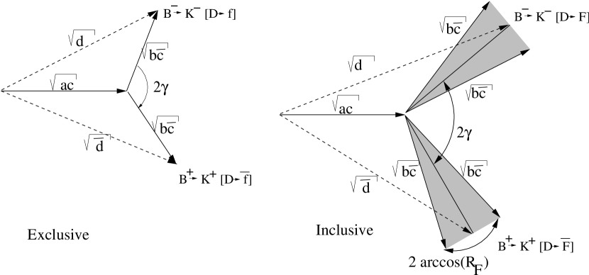
Figure 1: The geometric representation of Eqn. (LABEL:inclusive_d) and Eqn. (1).

As was pointed out by [4], that if you know $d$, $\bar{d}$, $ac$ and $b\bar{c}$ you can reconstruct the diagram (up to discrete ambiguities) and thus determine $\gamma$. In the exclusive case, however, you would also have to know $R_{F}$.

Even with exclusive states, this approach may not be practical because the determination of the small branching ratio $B^{-}\to K^{-}\bar{D}^{0}$ is difficult [5]. This can be circumvented if two distinct exclusive states are used since then one does have enough information to solve for all the strong phases and $\gamma$. This fails in the case of inclusive states due to the extra parameter, $R_{F}$.

At a $\psi(3770)$ charm factory [11] it is possible to determine $\zeta_{f}$ for an exclusive state [12] and $\zeta$ and $R_{F}$ for an inclusive final state [8, 9]. This is because the decay $\psi(3770)\to D^{0}\bar{D}^{0}$ leaves the final state $D^{0}$’s in an anti-symmetric flavor state therefore if one of the $D$-mesons decays to an inclusive state $F$ and the other to state $G$, the correlated rate [9] (again, assuming $D$ mixing is small [7]) is:

$$\Gamma(FG) = \Gamma_{0}\bigg{[}A_{F}^{2}\bar{A}_{G}^{2}+\bar{A}_{F}^{2}A_{G}^{2}$$ (4)

$$-2R_{F}R_{G}A_{F}\bar{A}_{F}A_{G}\bar{A}_{G}\cos(\zeta_{F}-\zeta_{G})\bigg{]}$$

where $\Gamma_{0}=\Gamma(\psi(3770)\to D^{0}\bar{D}^{0}$. If $G$ is a CPES with CP eigenvalue $\lambda_{G}=\pm 1$, then this reduces to:

$$\Gamma(FG) = \Gamma_{0}A_{G}^{2}\bigg{[}A_{F}^{2}+\bar{A}_{F}^{2}-2\lambda_{G}R_{F}A_{F}\bar{A}_{F}\cos(\zeta_{F})\bigg{]}$$

and if $F=G$ then

$$\Gamma(FF) = \Gamma_{0}A_{F}^{2}\bar{A}_{F}^{2}(1-R_{F}^{2})$$ (6)

Note in this latter case that if $R_{F}=1$ then $\Gamma(FF)=0$ by Bose symmetry.

Thus, let us suppose that $n$ distinct inclusive states as well as CP eigenstates are considered and all correlations are measured at a $\psi(3770)$ charm factory. The number of unknown parameters is $2n$ because there is $R_{F}$ and $\eta_{F}$ for each of the inclusive states. The number of correlations which can be measured is $n^{2}+2n$ as follows:

1. Each state can be correlated with any other state including itself giving $n(n+1)/2$ observables.

2. Each state can be correlated with the charge conjugate of any other state including itself giving $n(n+1)/2$ observables.

3. Each state can be correlated with a CPES giving $n$ observables.

There are therefore $n^{2}$ more observables than parameters. The same is also true if some of states are exclusive since an exclusive state has only one parameter ($\eta_{f}$) but the branching ratio $\psi(3770)\to ff$ is also automatically 0 by Bose symmetry so there is also one less observable.

3 Illustrative Example

Let us now consider some examples to illustrate how various combinations of final states can be taken together to determine $\gamma$.

First of all, let us consider two exclusive final states $f_{1}=K^{+}\pi^{-}$ and $f_{2}=K^{*+}\pi^{-}$ as well as CP=-1 eigenstates. The branching ratio $c(f_{1})=1.48\times 10^{-4}$ [13] while $\bar{c}(f_{1})=3.80\times 10^{-2}$ [13]; $c(f_{2})=1.7\times 10^{-4}$ while $\bar{c}(f_{1})=6.0\times 10^{-2}$ [13]. Note $c(f_{2})$ is not yet measured so we estimate it by multiplying $\bar{c}(f_{2})$ by $\tan^{4}\theta_{C}$. For illustrative purposes, we will take the ad-hoc values $\zeta_{f_{1}}=120^{\circ}$ and $\zeta_{f_{2}}=120^{\circ}$. We will take the branching ratio of $CPES-$ states to be $\sim 5\%$, roughly the rate of $D^{0}$ 2 body decays to $K_{S}$ and a pseudo-scalar or vector.

Figure 2: $\chi^{2}$ is plotted as a function of $\zeta$ using correlations at a $\psi(3770)$ factory using correlations between the exclusive modes considered in $f_{1}$ and $f_{2}$. The solid line is for the mode $f_{1}=K^{+}\pi^{-}$ while the dashed line is for the mode $f_{2}=K^{*+}\pi^{-}$.

In Fig. (2) we show the minimum value of $\chi^{2}$ at each possible value of $\zeta$ for each of the two exclusives states were we use the 6 possible correlations as discussed above (i.e. $f_{1}\times\bar{f}_{1}$, $f_{2}\times\bar{f}_{2}$, $f_{1}\times f_{2}$, $f_{1}\times\bar{f}_{2}$, $f_{1}\times CPES$, $f_{2}\times CPES$). To calculate $\chi^{2}$ we take $\hat{N}_{D}=(acceptance)\times(number~{}of~{}D^{0}\bar{D}^{0})=10^{7}$. Probably $\hat{N}_{D}\sim 100-300$ would roughly correspond to reasonable $3\sigma$ errors form CLEO-c.

Let us now see how well this can be used to determine $\gamma$. For the purpose of illustration, we will assume that $\zeta_{B}=-50^{\circ}$ and $\gamma=60^{\circ}$, which is consistent with the current CKM fits [14].

Figure 3: $\chi^{2}$ is plotted as a function of $\gamma$ for input generated assuming $\gamma=60^{\circ}$ and $\zeta_{B}=-50^{\circ}$ using various combinations of exclusive states with $\hat{N}_{B}=10^{9}$. The dotted curve uses only data from two $D$ decay modes: CPES- and $K^{*+}\pi^{-}$; the solid curve includes data from three modes: CPES-, $K^{*+}\pi^{-}$ and $K^{-}\pi^{+}$. The dot-dashed curve uses the same modes but correlation data from a $\psi(3770)$ factory with $\hat{N}_{D}=10^{7}$ is also included.

In Fig. (3) we show the minimum $\chi^{2}$ as a function of $\gamma$ for a number of combinations of the data sets assuming $\hat{N}_{B}=(number~{}of~{}B^{\prime}s)\times(Acceptance)=10^{9}$. Notice that the curves are symmetric with respect to $\gamma\to\pi-\gamma$ as well as $\gamma\to\pi+\gamma$ therefore there is ultimately a 4-fold ambiguity in the determination of $\gamma$ through this method.

The dotted curve shows the results where we just use $d$ and $\bar{d}$ for both $f_{2}=K^{*+}\pi^{-}$ and $CPES-$. Notice that the curve is pulled to 0 at a number of points due to the discrete ambiguities of the solution in this case because the four observables $d(CPES-)$, $\bar{d}(CPES-)$, $d(f_{2})$, $\bar{d}(f_{2})$ are determined by the four unknowns $b$, $\gamma$, $\eta_{B}$ and $\eta_{f_{2}}$. If we add another mode, $f_{1}=K^{-}\pi^{+}$ as is shown by the solid curve, the situation is improved since this adds two more observables, $d(f_{1})$ and $\bar{d}(f_{1})$ but only one more unknown, $\eta_{f_{1}}$. Clearly the ambiguities are largely lifted in fact. Finally, if we fit the B factory data jointly with the $\psi(3770)$ data discussed above we obtain the dash dotted curve where the parameters $\zeta_{f_{1}}$ and $\zeta_{f_{2}}$ are, in effect, determined from independently. Looking at the $3\sigma$ errors of $\gamma$ estimated by taking the intersection for the curve with $\chi^{2}=9$, we see that for the case of $f_{1}$ and $CPES-$, the error is $10^{\circ}$ (although there is additional confusion due to the multiple minima of the curve); for the case if $f_{1}$, $f_{2}$ and $CPES-$ the error is $9^{\circ}$ and for $f_{1}$, $f_{2}$ and $CPES-$ with charm factory data the error is $3.4^{\circ}$. In the last case the curve also smoothly funnels down to the correct value of $\gamma$ indicating that the convergence will scale well as data is improved.

Figure 4: $\chi^{2}$ is plotted as a function of $\gamma$ for input generated assuming $\gamma=60^{\circ}$ and $\zeta_{B}=-50^{\circ}$ for various combinations of inclusive states with $\hat{N}_{B}=10^{9}$ together with $\psi(3770)$ factory data. The solid curve uses only ${\cal F}$ and CPES-. The dashed line uses information from ${\cal F}_{1-3}$ together with CPES-.

Let us turn our attention now to the an inclusive case where we consider decays of the form ${\cal F}=\{K^{+}+X\}$. We will model this set of states using the model discussed in [9]. We shall also consider breaking down this set according to the energy of the $K^{+}$ where ${\cal F}_{1}$ has $E_{K}\leq 1.7GeV$, ${\cal F}_{2}$ has $1.7GeV\leq E_{K}\leq 4.7GeV$ and ${\cal F}_{3}$ has $4.7GeV<E_{K}$. In this model, $\zeta_{\cal F}=-11^{\circ}$, $\zeta_{{\cal F}_{1}}=-34^{\circ}$, $\zeta_{{\cal F}_{2}}=-86^{\circ}$ and $\zeta_{{\cal F}_{3}}=-30^{\circ}$, while $R_{\cal F}=.51$, $R_{{\cal F}_{1}}=.74$, $R_{{\cal F}_{2}}=.29$ and $R_{{\cal F}_{3}}=.91$.

If we fit $\gamma$ using $d$ and $\bar{d}$ for ${\cal F}$ and $CPES-$ together with charm factory data determining $R_{\cal F}$ and $\zeta_{F}$ we obtain the solid curve in Fig. (4). The corresponding $3\sigma$ error in $\gamma$ is $12^{\circ}$. If, however, we take the exact same data except we break ${\cal F}$ down into ${\cal F}_{1-3}$ we obtain the dashed curve in Fig. (4) with the corresponding error of $2.3^{\circ}$. The improvement is due to the fact that in breaking down the data we have increased the number of constraints compared to the number of unknown parameters. Of course the statistical errors on each of the $d$ and $\bar{d}$’s in the latter case will be larger. The improvement of the latter case with respect to the exclusive states is largely due to the fact that we have larger statistics overall. Clearly, as discussed in [9, 10], it is important to consider different strategies for breaking down inclusive data in order to obtain the best determination of $\gamma$.

4 Conclusion

In conclusion, I have shown how the strong phase properties of an inclusive decay of $D^{0}$ may be represented by two parameters, $R_{F}$ and $\zeta_{F}$. Correlated decays in a $\psi(3770)$ charm factory provide a means of obtaining these parameters. This information may be put to good use in obtaining the CKM phase $\gamma$ via $B^{-}\to K^{-}D^{0}$ so that a $\psi(3770)$ charm factory will proved invaluable information to interpret this data from $B$ factories.

References

- [1] N. Cabibbo, Phys. Rev. Lett. 10, 531 (1963); M. Kobayashi and T. Maskawa, Prog. Th. Phys. 49, 652 (1973).
- [2] K. Abe et al (BELLE Collab), Phys. Rev. D 66, 071102 (2002)
- [3] B. Aubert et al (BABAR Collab), Phys. Rev. Lett. 89, 201802 (2002).
- [4] M. Gronau and D. Wyler, Phys. Lett. B265 (1991); M. Gronau and D. London., Phys. Lett. B253, 483 (1991).
- [5] D. Atwood, I. Dunietz and A. Soni, Phys. Rev. Lett. 78, 3257 (1997); Phys. Rev. D 63, 036005 (2001).
- [6] Y. Grossman, Z. Ligeti and A. Soffer, hep-ph/0210433;
- [7] J. P. Silva and A. Soffer, Phys. Rev. D 61, 112001 (2000).
- [8] D. Atwood and A. Soni, arXiv:hep-ph/0206045.
- [9] D. Atwood and A. Soni, arXiv:hep-ph/0304085.
- [10] A. Giri, Y. Grossman, A. Soffer and J. Zupan, arXiv:hep-ph/0303187.
- [11] I. Shipsey, arXiv:hep-ex/0207091.
- [12] A. Soffer, arXiv:hep-ex/9801018.
- [13] K. Hagiwara et al. [Particle Data Group Collaboration], Phys. Rev. D 66, 010001 (2002).
- [14] F. J. Gilman, K. Keinknecht and B. Renk, in Review of Particle Properties K. Hagiwara et al. [Particle Data Group Collaboration], Phys. Rev. D 66, 010001-113 (2002).