Abstract

We develop a new systematic procedure for the Regge limit in perturbative QCD to arbitrary logarithmic order. The formalism relies on the IR structure and the gauge symmetry of the theory. We identify leading regions in loop momentum space responsible for the singular structure of the amplitudes and perform power counting to determine the strength of these divergences. Using a factorization procedure introduced by Sen, we derive a sum of convolutions in transverse momentum space over soft and jet functions, which approximate the amplitude up to power-suppressed corrections. A set of evolution equations generalizing the BFKL equation and controlling the high energy behavior of the amplitudes to arbitrary logarithmic accuracy is derived. The general method is illustrated in the case of leading logarithmic gluon reggeization and BFKL equation.

1 Introduction

The study of semihard processes within the framework of gauge quantum field theories has a long history. For reviews see Refs. [1]-[3]. The defining feature of such processes is that they involve two or more hard scales, compared to $\Lambda_{\rm QCD}$, which are strongly ordered relative to each other. The perturbative expansions of scattering amplitudes for these processes must be resummed since they contain logarithmic enhancements due to large ratios of the scales involved. One of the most important examples is elastic $2\rightarrow 2$ particle scattering in the Regge limit, $s\gg|t|$ (with $s$ and $t$ the usual Mandelstam variables). It is this process that we investigate in this paper. We extend the techniques developed in Refs. [4] and [5] and devise a new systematic method for evaluation of QCD scattering amplitudes in the Regge limit to arbitrary logarithmic accuracy.

The problem of the Regge limit in quantum field theory was first tackled in the case of fermion exchange amplitude within QED in Ref. [6]. Here it was found that the positive signature amplitude takes a reggeized form up to the two loop level in Leading Logarithmic (LL) approximation. In Ref. [7] the calculations were extended to higher loops, and the imaginary part of the Next-to-Leading Logarithms (NLL) was also obtained. The analysis in Refs. [6] and [7] was performed in Feynman gauge. It was realized in Ref. [8] that a suitable choice of gauge can simplify the class of diagrams contributing at LL. The common feature of all this work was the use of fixed order calculations. To verify that the pattern of low order calculations survives at higher orders, a method to demonstrate the Regge behavior of amplitudes to all orders is necessary. This analysis was provided by A. Sen in Ref. [4], in massive QED. Sen developed a systematic way to control the high energy behavior of fermion and photon exchange amplitudes to arbitrary logarithmic accuracy. The formalism relies heavily on the IR structure and gauge invariance of QED and provides a proof of the reggeization of a fermion at NLL to all orders in perturbation theory.

The resummation of color singlet exchange amplitudes in non-abelian gauge theories in LL was achieved in the pioneering work of Ref. [9], where the reggeization of a gluon in LL was also demonstrated. The evolution equations resumming LL in the case of three gluon exchange was derived in Ref. [10]. In Ref. [5], $n$-gluon exchange amplitudes in QCD at LL level were studied and a set of evolution equations governing the high energy behavior of these amplitudes was obtained at LL. A different approach was undertaken in Ref. [11]. Here $n\rightarrow m$ amplitudes were studied in SU(2) Higgs model with spontaneous symmetry breaking. Starting with the tree level amplitudes, an iterative procedure was developed, which generates a minimal set of terms in the perturbative expansion that have to be taken into account in order to satisfy the unitarity requirement of the theory. See also Ref. [12]. The extension of the BFKL formalism to NLL spanned over a decade. For a review see Ref. [13]. The building blocks of NLL BFKL are the emissions of two gluons or two quarks along the ladder, Ref. [14], one loop corrections to the emission of a gluon along the ladder, Ref. [15], and the two loop gluon trajectory, Refs. [16], [17], [18] and [19]. The particular results were put together in Ref. [20]. In Ref. [21], the trajectory for the fermion at NLL was evaluated by taking the Regge limit of the explicit two loop partonic amplitudes, Ref. [22].

Besides the NLO perturbative corrections to the BFKL kernel a variety of approaches have been developed for unitarization corrections, Refs. [23, 24, 25], which extend the BFKL formalism by incorporating selected higher-order corrections. The procedure proposed in this paper, in a way, places these approaches in an even more general context. In principle, it makes it possible to find the scattering amplitudes to arbitrary logarithmic accuracy and to determine the evolution kernels to arbitrary fixed order in the coupling constant. The formalism contains all color structures and, of course, the construction of the amplitude to any given level requires the computation of the kernels and the solution of the relevant equations.

The paper is organized as follows. In Sec. 2 we discuss the kinematics of the partonic process under study and the gauge used. In Sec. 3 we identify the leading regions in internal momentum space, which produce logarithmic enhancements in the perturbation series. After identifying these regions, we perform power counting to verify that the singularity structure of individual diagrams is at worst logarithmic. The leading regions lead to a factorized form for the amplitude (First Factorized Form). It consists of soft and jet functions, convoluted over soft loop momenta, which can still produce logarithms of $s/|t|$. In Sec. 4 we study the properties of the jet functions appearing in the factorization formula for the amplitude. We show how the soft gluons can be factored from the jet functions. In Sec. 5 we demonstrate how to express systematically the amplitude as a convolution in transverse momenta. In this form all the large logarithms are organized in jet functions and the soft transverse momenta integrals do not introduce any logarithms of $s/|t|$ (Second Factorized Form). We derive evolution equations that enable us to control the high energy behavior of the scattering amplitudes. In Sec. 6, we illustrate the general methods valid to all logarithmic accuracy in the case of LL and NLL in the amplitude and we examine the evolution equations at LL. Some technical details are discussed in appendices A - E. The first appendix treats power counting for regions of integration space where internal loop momenta become much larger than the momentum transfer. In Appendix B we illustrate the origin of special vertices encountered in the paper. In Appendix C we show a systematic expansion for the amplitude leading to the first factorized form. In Appendix D we list the Feynman rules used throughout the text. Finally, in Appendix E we demonstrate the origin of extra soft momenta configurations (Glauber region) which need to be considered in the analysis of amplitudes in the Regge limit.

2 Kinematics and Gauge

We analyze the amplitude for the elastic scattering of massless quarks

$$q(p_{A},r_{A})+q^{\prime}(p_{B},r_{B})\rightarrow q(p_{A}-q,r_{1})+q^{\prime}(p_{B}+q,r_{2}),$$ (1)

within the framework of perturbative QCD in the kinematic region $s\gg-t$ (Regge limit), where $s=(p_{A}+p_{B})^{2}$ and $t=q^{2}$ are the usual Mandelstam variables. We stress, however, that the results obtained below apply to arbitrary elastic two-to-two partonic process. We pick process (1) for concreteness only. The arguments in Eq. (1) label the momenta and the colors of the quarks (we do not exhibit the dependence on the polarizations). We choose to work in the center-of-mass (c.m.) where the momenta of the incoming quarks and the momentum transfer have the following components

$$p_{A} = \left(\sqrt{\frac{s}{2}},0^{-},0_{\perp}\right),$$

$$p_{B} = \left(0^{+},\sqrt{\frac{s}{2}},0_{\perp}\right),$$

$$q = (0^{+},0^{-},q_{\perp}).$$ (2)

Strictly speaking $q^{\pm}=\pm|t|/\sqrt{2s}$, so the $q^{\pm}$ components vanish in the Regge limit only.

In the color basis

$$b_{\bf 1} = \delta_{r_{A},\,r_{1}}\delta_{r_{B},\,r_{2}},$$

$$b_{\bf 8} = -\frac{1}{2N_{c}}\delta_{r_{A},\,r_{1}}\delta_{r_{B},\,r_{2}}+\frac{1}{2}\delta_{r_{A},\,r_{2}}\delta_{r_{B},\,r_{1}},$$ (3)

with $N_{c}$ the number of colors, we can view the amplitude for process (1) as a two dimensional vector in color space

$$A=\left(\begin{array}[]{c}A_{\bf 1}\\ A_{\bf 8}\end{array}\right),$$ (4)

where $A_{\bf 1}$ and $A_{\bf 8}$ are defined by the expansion

$$A_{\,r_{A}\,r_{B},\;r_{1}\,r_{2}}=A_{\bf 1}\,(b_{\bf 1})_{r_{A}\,r_{B},\;r_{1}\,r_{2}}+A_{\bf 8}\,(b_{\bf 8})_{r_{A}\,r_{B},\;r_{1}\,r_{2}}.$$ (5)

Since the amplitude is dimensionless and all particles are massless, its components can depend, in general, on the following variables

$$A_{i}\equiv A_{i}\left(\frac{s}{{\mu}^{2}},\frac{t}{{\mu}^{2}},{\alpha}_{s}({\mu}^{2}),\epsilon\right)\hskip 56.9055pt\mbox{for}\;i={\bf 1},{\bf 8},$$ (6)

where $\mu$ is a scale introduced by regularization. We use dimensional regularization in order to regulate both infrared (IR) and ultraviolet (UV) divergences with $D=4-2\varepsilon$ the number of dimensions. Choosing the scale ${\mu}^{2}=s$, the strong coupling, ${\alpha}_{s}(\mu)$, is small. However, in general, an individual Feynman diagram contributing to the process (1) at $r$-loop order can give a contribution as singular as $(s/t)\,{\alpha}_{s}^{r+1}{\ln}^{2r}(-s/t)$. In Sec. 5.3 we will confirm that there is a cancellation of all terms proportional to the $i$-th logarithmic power for $i=r+1,\ldots,2r$ at order ${\alpha}_{s}^{r+1}$ in the perturbative expansion of the amplitude. Hence at $r$ loops the amplitude is enhanced by a factor $(s/t)\,{\alpha}_{s}^{r+1}\ln^{r}(-s/t)$, at most. In order to get reliable results in perturbation theory we must, nevertheless, resum these large contributions. In the $k$-th nonleading logarithmic approximation one needs to resum all the terms proportional to $(s/t)\,{\alpha}_{s}^{r+1}\ln^{r-j}(-s/t),\;\;j=0,\ldots,k$ at $r$-loop level.

We perform our analysis in the Coulomb gauge, where the propagator of a gluon with momentum $k$ has the form

$$-i\,{\delta}_{ab}\;\frac{N_{\alpha\beta}(k,{\bar{k}})}{k^{2}+i\epsilon}\equiv-i\,{\delta}_{ab}\;\frac{1}{k^{2}+i\epsilon}\left(g_{\alpha\beta}-\frac{k_{\alpha}\,{\bar{k}}_{\beta}+{\bar{k}}_{\alpha}\,k_{\beta}-k_{\alpha}\,k_{\beta}}{k\cdot{\bar{k}}}\right),$$ (7)

in terms of the vector

$$\bar{k}=k-(k\cdot{\eta})\,\eta,$$ (8)

with

$$\eta=\left(\frac{1}{\sqrt{2}},\frac{1}{\sqrt{2}},0_{\perp}\right),$$ (9)

an auxiliary four-vector defined in the partonic c.m. frame. The numerator of the gluon propagator satisfies the following identities

$$k^{\alpha}\,N_{\alpha\beta}(k,{\bar{k}}) = k^{2}\,\frac{k_{\beta}-{\bar{k}}_{\beta}}{k\cdot{\bar{k}}},$$

$${\bar{k}}^{\alpha}\,N_{\alpha\beta}(k,{\bar{k}}) = 0.$$ (10)

The first equality in Eq. (2) is the statement that the nonphysical degrees of freedom do not propagate in this gauge. For use below, we list the components of the gluon propagator:

$$N^{+-}(k)=N^{-+}(k) = \frac{k^{+}k^{-}-k_{\perp}^{2}}{k\cdot\bar{k}},$$

$$N^{++}(k)=N^{--}(k) = \frac{k^{+}k^{-}}{k\cdot\bar{k}},$$

$$N^{\pm\;i}(k)=N^{i\;\pm}(k) = \pm\frac{(k^{-}-k^{+})k^{i}}{2k\cdot\bar{k}},$$

$$N^{i\;j}(k)=N^{j\;i}(k) = g^{ij}-\frac{k^{i}k^{j}}{k\cdot\bar{k}}.$$ (11)

We note that these are symmetric functions under the transformation $k^{\pm}\rightarrow-k^{\pm}$, except for the components $N^{\pm\;i}=N^{i\;\pm}$, which are antisymmetric under this transformation. It was demonstrated in Ref. [26] that QCD is renormalizable in Coulomb gauge, by considering a class of gauges which interpolates between the covariant (Landau) and the physical (Coulomb) gauge.

3 Leading Regions, Power Counting

In order to resum the Regge logarithms, we need to identify the regions of integration in the loop momentum space that give rise to singularities in the limit $t/s\rightarrow 0$. We follow the method developed in Refs. [27, 28], which begins with the identification of the relevant regions in momentum space.

3.1 Singular contributions and reduced diagrams

The singular contributions of a Feynman integral come from the points in loop momentum space where the integrand becomes singular due to the vanishing of propagator denominators. However, in order to give a true singularity the integration variables must be trapped at such a singular point. Otherwise we can deform the integration contour away from the dangerous region. These singular points are called pinch singular points. They can be identified with the following regions of integration in momentum space,

1. soft momenta, with scaling behavior $k^{\mu}\sim\sigma\,\sqrt{s}$ for all components ($\sigma\ll 1$),

2. momenta collinear to the momenta of the external particles, with scaling behavior
   $k^{+}\sim\sqrt{s},\;k^{-}\sim\lambda\,\sqrt{s},\;|k_{\perp}|\sim{\lambda}^{1/2}\,\sqrt{s}$ for the particles moving in the $+$ direction and
   $k^{+}\sim\lambda\,\sqrt{s},\;k^{-}\sim\sqrt{s},\;|k_{\perp}|\sim{\lambda}^{1/2}\,\sqrt{s}$ for the particles moving in the $-$ direction,

3. so-called Glauber or Coulomb momenta, Ref. [29], with scaling behavior $k^{\pm}\sim{\sigma}^{\pm}\,\sqrt{s}$,   $|k_{\perp}|\sim\sigma\,\sqrt{s}$, where $\lambda\lesssim{\sigma}^{\pm}\lesssim\sigma$, and where the scaling factors $\lambda,\sigma$ satisfy the strong ordering $\lambda\ll\sigma\ll 1$ (The origin of this region is illustrated in Appendix E.),

4. hard momenta, having the scaling behavior $k^{\mu}\sim\sqrt{s}$ for all components.

The extra gauge denominators $1/(k\cdot{\bar{k}})$ originating from the numerators of the gluon propagator, Eq. (7), do not alter the classification of the pinch singular points mentioned above. Actually, only the subsets 1 and 3 in the above classification can be produced due to the extra gauge denominators.

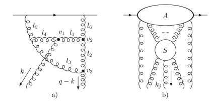
With every pinch singular point, we may associate a reduced diagram, which is obtained from the original diagram by contracting all hard lines (subset 4) at the particular singular point. As shown in Refs. [27, 28, 30] the reduced diagram corresponding to a given pinch singular point must describe a real physical process, with each vertex of the reduced diagram representing a real space-time point. This physical interpretation suggests two types of reduced diagrams contributing to the process (1), shown in Fig. 1.

Figure 1: The reduced diagrams a) and c) contributing to the amplitude. Diagram b) represents a decomposition of diagram a) for the purpose of power counting.

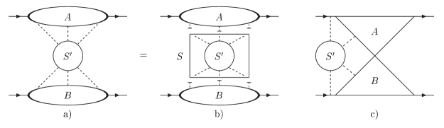
The jet $A$($B$) contains lines whose momenta represent motion in the $+\;(-)$ direction. The lines included in the blob $S^{\prime}$ and the lines coming out of it are all soft (configurations 1 and 3 in the classification of loop momenta described above). These two oppositely moving (virtual) jets may interact through the exchange of soft lines, Fig. 1a, and/or they can meet at one or more space-time points, Fig. 1c.

Having found the most general reduced diagrams giving the leading behavior of the amplitude for process (1) in the Regge limit, we can estimate the strength of the IR divergence of the integral near a given pinch singular point. First we restrict ourselves to cases involving subsets 1 and 2 from the classification of loop momenta above. To do so, we count powers in the scaling variables $\lambda$ and $\sigma$.

The scaling behavior of these loop momenta implies that every soft loop momentum contributes a factor ${\sigma}^{4}$, every jet loop momentum gives rise to the power ${\lambda}^{2}$, every internal soft boson (fermion) line provides a contribution ${\sigma}^{-2}$ (${\sigma}^{-1}$) and every internal jet line (fermionic or bosonic) scales as ${\lambda}^{-1}$. In addition, there can be suppression factors arising from the numerators of the propagators associated with internal lines and from internal vertices. As pointed out in Ref. [27], in physical gauges each three-point vertex connecting three jet lines is associated with a numerator factor that vanishes at least linearly in the components of the transverse jet momenta, and therefore provides a suppression ${\lambda}^{1/2}$.

We are now ready to estimate the power of divergence corresponding to the reduced diagrams describing our process. First we restrict ourselves to the case shown in Fig. 1a. As indicated schematically in Fig. 1b, we can perform the power counting for the jets and for the soft part separately. All soft propagators and all soft loop momenta are included in the soft subdiagram $S$. The superficial degree of IR divergence of the reduced diagram $R$ from Fig. 1a and Fig. 1b can then be written as

$$\omega(R)=\omega(A)+\omega(B)+\omega(S),$$ (12)

where the external lines and loops of $S^{\prime}$ are included in $S$. For $\omega(R)>0$ the overall integral is finite, while $\omega(R)\leq 0$ corresponds to an IR divergent integral. When $\omega(R)=0$, the integral diverges logarithmically. Here we set $\lambda\sim\sigma$ for power counting purposes. We come back to the effect of relaxing this condition in connection with a discussion of item 3, Glauber regions, in our list of singular momentum configurations.

3.2 Power counting

In this subsection, we consider the case when all vertices in a diagram are elementary only, that is, without contracted subdiagrams carrying large loop momenta. In Appendix A we show that our conclusions are unchanged by contracted vertices.

We perform the power counting for the soft part $S$ first. Let $f,b$ be the number of fermion, boson lines external to $S^{{}^{\prime}}$ and let $E=f+b$. The superficial degree of divergence for $S$, found by summing powers of $\sigma$, can be written

$$\omega(S)=4(E-2)-2b-f+2+\omega(S^{{}^{\prime}}),$$ (13)

where the first term is due to loop integrations linking $S^{\prime}$ to the jets, while the second and the third terms originate from propagators associated with the bosonic and fermionic lines, respectively, connecting the jets $A$, $B$ and the soft part $S^{\prime}$. The term $+2$ is introduced because we are resumming only leading power corrections proportional to $s/t$ and therefore we exclude the overall factor $s/t$ from the power counting. Since the lines entering $S^{\prime}$ are soft, we obtain the superficial degree of divergence for $S^{\prime}$ simply from dimensional analysis. It is given by

$$\omega(S^{{}^{\prime}})=4-b-3f/2.$$ (14)

Combining Eqs. (13) and (14), the superficial degree of infrared divergence for the soft part $S$ is then

$$\omega(S)=b+3f/2-2.$$ (15)

Before carrying out the jet power counting, we introduce some notation. Let $E_{A}$ be the number of soft lines attached to jet $A$; $I$ is the total number of jet internal lines; $v_{\alpha}$ is the number of $\alpha$-point vertices connecting jet lines only; $w_{\alpha}$ has a meaning similar to $v_{\alpha}$, with the difference that every vertex counted by $w_{\alpha}$ has at least one soft line attached to it. These are the vertices that connect the jet $A$ to the soft part $S$. Finally, $L$ denotes the number of loops internal to jet $A$. As noted above, we will perform the power counting for the case when the scaling factor for the soft momenta, $\sigma$, is of the same order as the scaling factor for jet $A$ momenta. When the scaling factors are different we encounter subdivergencies, which can be analyzed the same way as described below. We also assume that there are no internal and external ghost lines included in the jet function. Later we will discuss the effect of adding ghost lines.

The superficial degree of divergence for jet $A$ can now be expressed as

$$\omega(A)=2L-I+v_{3}/2.$$ (16)

The last term represents the suppression factor associated with the three point vertices. We denote the total number of vertices internal to jet $A$ by

$$v=\sum_{\alpha}(v_{\alpha}+w_{\alpha}).$$ (17)

Next we use the Euler identity relating the number of loops, internal lines and vertices of jet $A$

$$L=I-v+1,$$ (18)

and the relation between the number of lines and the number of vertices

$$2I+E_{A}+2=\sum_{\alpha}\alpha(v_{\alpha}+w_{\alpha}).$$ (19)

Using Eqs. (16)-(19) we arrive at the following form for the superficial degree of divergence for jet $A$

$$\omega(A)=1-(E_{A}+w_{3})/2+\sum_{\alpha\geq 5}(\alpha-4)(v_{\alpha}+w_{\alpha})/2.$$ (20)

Since every vertex counted by $w_{\alpha}$ connects at least one external soft line, we have the condition

$$E_{A}\geq w_{3}+\sum_{{\alpha}\geq 4}w_{\alpha}.$$ (21)

The equality holds when there is no vertex with two or more soft lines attached to it. Combining Eqs. (20)-(21) we arrive at the following lower bound on the superficial degree of divergence for jet $A$:

$$\omega(A)\geq 1-E_{A}+\sum_{{\alpha}\geq 4}w_{\alpha}/2+\sum_{\alpha\geq 5}(\alpha-4)(v_{\alpha}+w_{\alpha})/2.$$ (22)

The third and the last term in Eq. (22) are always positive or zero and hence

$$\omega(A)\geq 1-E_{A}.$$ (23)

A similar result holds for jet $B$, and therefore the superficial degree of collinear divergence for jets $A$ and $B$ is

$$\omega(A)+\omega(B)\geq 2-E,$$ (24)

with $E=E_{A}+E_{B}$ as in Eq. (13). Combining the results for soft and jet power counting, Eqs. (15) and (24), respectively in Eq. (12), we finally obtain the superficial degree of IR divergence for the reduced diagram in Fig. 1a,

$$\omega(R)\geq f/2.$$ (25)

This condition says that we can have at worst logarithmic divergences, provided no soft fermion lines are exchanged between the jets $A$ and $B$. We can therefore conclude that a reduced diagram from Fig. 1a containing elementary vertices can give at worst logarithmic enhancements in perturbation theory. In order for the divergence to occur, the following set of conditions must be satisfied:

1. There is an exchange of soft gluons between the jets $A$ and $B$ only, with no soft fermion lines attached to the jets.

2. The jets $A$ and $B$ contain $3$ and $4$ point vertices only, see Eq. (22).

3. Soft gluons are connected to jets only through $3$ point vertices, Eq. (22), and at most one soft line is attached to each vertex inside the jets, Eq. (21).

4. In the reasoning above we have assumed that there is no suppression factor associated with the vertices where soft and jet lines meet. In order for this to be true, the soft gluons must be connected to the jet $A$($B$) lines via the $+(-)$ components of the vertices.

Next we consider adding ghost lines to the jet functions. As we review in Appendix D, the propagator for a ghost line with momentum $k$ is proportional to $1/(k\cdot{\bar{k}})$. Hence every internal ghost line belonging to the jet gives a contribution which is power suppressed as $1/s$. Since the numerator factors do not compensate for this suppression, we can immediately conclude that the jet functions cannot contain internal or external ghost lines at leading power.

So far we have not taken into account the possibility when the soft loop momenta are pinched by the singularities of the jet lines. This situation allows different components of soft momenta to scale differently. For example, a minus component of soft momentum can scale as the minus component of jet $A$ momentum $\lambda$, while the rest of the soft momentum components may scale as $\sigma$, where $\lambda\ll\sigma\ll 1$. The origin of these extra pinches is illustrated in Appendix E.

Let us see what happens when we attach the ends of a gluon line with this extra pinch to jet $A$ at one end and the soft subdiagram $S$ at the other end. The integration volume for this soft loop momentum scales as $\lambda{\sigma}^{3}$. The soft gluon denominator gives a factor ${\sigma}^{-2}$. If this soft gluon is connected to the soft part at a $4$-point vertex, there is no new denominator in the soft part. On the other hand, if the soft gluon is attached to the soft part via a $3$-point vertex then the extra denominator including the numerator suppression factors scales as ${\sigma}^{-1}$. The new jet line scales as ${\lambda}^{-1}$ as long as the condition ${\lambda}^{1/2}\gtrsim\sigma$ is obeyed; otherwise, we have the scaling ${\sigma}^{-2}$ for the extra jet line. For ${\lambda}^{1/2}\gtrsim\sigma$ the Glauber region produces logarithmic infrared divergence. When ${\lambda}^{1/2}\lesssim\sigma$, the overall scaling factor $\lambda/{\sigma}^{2}$ indicates power suppressed contribution.

Let us now investigate another possibility, when the soft gluon connects jet $A$ and jet $B$ directly and its momentum is pinched by the singularities of the jet $A$ and the jet $B$ lines. Denoting the scaling factors of jet $A$ and jet $B$ as ${\lambda}_{A}$ and ${\lambda}_{B}$, respectively, the integration volume provides the factor ${\lambda}_{A}{\lambda}_{B}{\sigma}^{2}$ and the soft gluon denominator contributes the power ${\sigma}^{-2}$. The extra jet $A$ and jet $B$ denominators scale as ${\lambda}_{A}^{-1}$ and ${\lambda}_{B}^{-1}$, provided ${\lambda}_{A}^{1/2}\gtrsim\sigma$ and ${\lambda}_{B}^{1/2}\gtrsim\sigma$. For ${\lambda}_{A,B}^{1/2}\lesssim\sigma$ both extra jet denominators provide the scaling factor ${\sigma}^{-2}$. When ${\lambda}_{A,B}^{1/2}\gtrsim\sigma$, the power counting suggests logarithmically divergent integrals.

We have therefore verified that when the softest component of a soft line satisfies the ordering ${\sigma}^{2}\lesssim\lambda\lesssim\sigma$, the Glauber (Coulomb) momenta produce logarithmically IR divergent integrals and need to be taken into an account when identifying enhancements in perturbation series. The analysis demonstrated above for the case of one Glauber gluon can be extended to the situation with arbitrary number of Glauber gluons. This follows from dimensional analysis, in a similar fashion as the treatment of purely soft loop momenta above.

We conclude that the reduced diagram in Fig. 1a is at most logarithmically IR divergent, modulo the factor $s/|t|$. The reduced diagram in Fig. 1b looses one small denominator compared to the reduced diagram in Fig. 1a and since we are working in physical gauge, this loss cannot be compensated by a large kinematical factor coming from the numerator. Hence the reduced diagram in Fig. 1b is power suppressed compared to the reduced diagram in Fig. 1a, and we do not need to consider it at leading power.

Finally, let us discuss the scale of the soft momenta. In the case of soft exchange lines, each gluon propagator supplies a factor $1/({\sigma}^{2}\,{s})$, which we want to keep at or below the order $t$ in the leading power approximation. Thus the size of the scale is fixed to be $\sigma\sim\sqrt{|t|}/\sqrt{s}$. In the case of soft lines which are attached to jet $A$ or to jet $B$ only, the scaling factor lies in the interval $(\sqrt{|t|}/\sqrt{s},1)$. In the case of Glauber momenta, we again need $\sigma\sim\sqrt{|t|}/\sqrt{s}$. Then the condition ${\lambda}^{1/2}\gtrsim\sigma$, which is necessary for the logarithmic enhancement, implies that the scaling factors for $+$ and $-$ components of the Glauber (Coulomb) momenta can go down to $|t|/s$, the scale of the small components of jet momenta. Additionally, we should note that soft and jet subdiagrams that do not carry the momentum transfer may approach the mass shell ($\lambda,\ \sigma\rightarrow 0$). Such lines produce true infrared divergences, which we assume are made finite by dimensional regularization to preserve the gauge properties that we will use below. The same power counting as above shows that these divergences are also at worst logarithmic.

Figure 2: Jet $A$ moving in the $+$ direction (a) and jet $B$ moving in the $-$ direction (b).

3.3 First factorized form

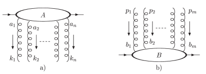
The analysis of the previous subsection suggests the following decomposition of the leading reduced diagram from Fig. 1a. Let us denote the $(n+2)$-point and $(m+2)$-point Green functions, 1PI in external soft gluon lines, corresponding to jet $A$, $J_{(A)\,{\mu}_{1}\ldots\,{\mu}_{n}}^{(n)\,a_{1}\ldots\,a_{n}}(p_{A},q,\eta;k_{1},\ldots,k_{n})$, Fig. 2a, and to jet $B$, $J_{(B)\,{\nu}_{1}\ldots\,{\nu}_{m}}^{(m)\,b_{1}\ldots\,b_{m}}(p_{B},q,\eta;p_{1},\ldots,p_{m})$, Fig. 2b, respectively. The jet function $J_{(A)}^{(n)}$ ($J_{(B)}^{(m)}$) also depends on the color of the incoming and outgoing partons $r_{A}$, $r_{1}$ ($r_{B}$, $r_{2}$), as well as on their polarizations ${\lambda}_{A}$, ${\lambda}_{1}$ (${\lambda}_{B}$, ${\lambda}_{2}$), respectively. In order to avoid making the notation even more cumbersome we do not exhibit this dependence explicitly. In addition the dependence of $J_{(A)}^{(n)}$ and $J_{(B)}^{(m)}$ on the renormalization scale $\mu$ and the running coupling ${\alpha}_{s}(\mu)$ is understood. The jet functions also depend on the following parameters: the gauge fixing vector $\eta$, Eq. (9), of the Coulomb gauge, the four momenta of the external soft gluons attached to jet $A$ ($B$), $k_{1},\ldots,k_{n}$ ($p_{1},\ldots,p_{m}$), and the Lorentz and color indices of the soft gluons attached to the jet $A$ ($B$), ${\mu}_{1},\ldots,{\mu}_{n}$; $a_{1},\ldots,a_{n}$ (${\nu}_{1},\ldots,{\nu}_{m}$; $b_{1},\ldots,b_{m}$). The momenta of the soft gluons attached to the jets $A$ and $B$ satisfy the constraints $\sum_{i=1}^{n}k_{i}=q$ and $\sum_{j=1}^{m}p_{j}=q$.

According to the results of the power counting, the soft gluons couple to jet $A$ via the minus components of their polarizations, and to jet $B$ via the plus components of their polarizations. Therefore, only the following components survive in the leading power approximation

$$J_{A}^{(n)\,a_{1}\ldots\,a_{n}}(p_{A},q,\eta,v_{B};k_{1},\ldots,k_{n}) \equiv \left(\prod^{n}_{i=1}v_{B}^{{\mu}_{i}}\right)J^{(n)\,a_{1}\ldots\,a_{n}}_{(A)\,{\mu}_{1}\ldots\,{\mu}_{n}}(p_{A},q,\eta;k_{1},\ldots,k_{n}),$$

$$J_{B}^{(m)\,b_{1}\ldots\,b_{m}}(p_{B},q,\eta,v_{A};p_{1},\ldots,p_{m}) \equiv \left(\prod^{m}_{i=1}v_{A}^{{\nu}_{i}}\right)J^{(m)\,b_{1}\ldots\,b_{m}}_{(B)\,{\nu}_{1}\ldots\,{\nu}_{m}}(p_{B},q,\eta;p_{1},\ldots,p_{m}),$$ (26)

where we have defined light-like momenta in the plus direction $v_{A}=(1,0,0_{\perp})$ and in the minus direction $v_{B}=(0,1,0_{\perp})$. We can now write the contribution to the reduced diagram in Fig. 1a, and hence to the amplitude for process (1), in the form

$$A = \sum_{n,m}\int\left(\prod^{n-1}_{i=1}\mathrm{d}^{D}k_{i}\right)\,\int\left(\prod^{m-1}_{j=1}\mathrm{d}^{D}p_{j}\right)\,J_{A}^{(n)\,a_{1}\ldots\,a_{n}}(p_{A},q,\eta,v_{B};k_{1},\ldots,k_{n})$$ (27)

$$\times S^{(n,m)}_{a_{1}\ldots\,a_{n},b_{1}\ldots\,b_{m}}(q,\eta,v_{A},v_{B};k_{1},\ldots,k_{n};p_{1},\ldots,p_{m})$$

$$\times J_{B}^{(m)\,b_{1}\ldots\,b_{m}}(p_{B},q,\eta,v_{A};p_{1},\ldots,p_{m}),$$

where the sum over repeated color indices is understood. Corrections to Eq. (27) are suppressed by positive powers of $t/s$. The jet functions $J_{A,B}$ are defined in Eq. (3.3) in the leading power accuracy. The internal loop momenta of the jets $A$, $B$ and of the soft function $S$ are integrated over. The soft function will, in general, include delta functions setting some of the momenta $k_{1},\ldots\,,k_{n}$ and color indices $a_{1},\ldots\,,a_{n}$ of jet function $J_{A}$ to the momenta $p_{1},\ldots\,,p_{m}$ and to the color indices $b_{1},\ldots\,,b_{m}$ of jet function $J_{B}$. The construction of the soft function $S$ is described in Appendix C. For a given Feynman diagram there exist many reduced diagrams of the type shown in Fig. 1a, and one has to be careful in systematically expanding this diagram into the terms that have the form of Eq. (27). This systematic method can be achieved using the “tulip-garden” formalism first introduced in Ref. [32] and used in a similar context in Ref. [4]. For convenience of the reader we summarize this procedure in Appendix C.

Let us now identify the potential sources of the enhancements in $\ln(s/|t|)$ of the amplitude given by Eq. (27). If we integrate over the internal momenta of the jet functions then we can get $\ln((p_{A}\cdot\eta)^{2}/|t|)$ from $J_{A}$ and $\ln((p_{B}\cdot\eta)^{2}/|t|)$ from $J_{B}$. In addition, according to the results of the power-counting, Eq. (23), we know that the jet function with $n$ external soft gluons diverges as $1/{\lambda}^{n-1}$. After performing the integrals over the minus components of the external soft gluon lines attached to jet $A$ and over the plus components of the external soft gluons connected to jet $B$, these divergent factors are potentially converted into logarithms of $\ln((p_{A}\cdot\eta)^{2}/|t|)$ and $\ln((p_{B}\cdot\eta)^{2}/|t|)$, respectively. Our goal will be to separate the full amplitude into a convolution over parameters that do not introduce any further logarithms of the form $\ln(s/|t|)$. This task will be achieved in Sec. 5.1. In the following section, we analyze the characteristics of the jet functions.

4 The Jet Functions

In this section we study the properties of the jet functions $A$, $B$ given by Eq. (3.3) since, as Eq. (27) suggests, they will play an essential role in later analysis. Since the methods for both jet functions are similar we restrict our analysis to jet $A$ only; jet $B$ can be worked out in the same way. In Sec. 4.1 we examine the properties of jet $A$ when the minus component of one of its external soft gluon momenta is of order $\sqrt{|t|}$. In Sec. 4.2 we find the variation of jet $A$ with respect to the gauge fixing vector $\eta$, and finally in Sec. 4.3 we examine the dependence of jet $A$ on the plus component of a soft gluon momentum attached to this jet.

4.1 Decoupling of a soft gluon from a jet

According to the results of power counting above, soft gluons attach to lines in jet $A$ via the minus components of their polarization. Following the technique of Grammer and Yennie [33] we decompose the vertex at which the $j$th gluon is connected to jet A. We start with a trivial rewriting of $J_{A}$ in Eq. (3.3)

Figure 3: a) Decoupling of a $K$ gluon from jet $A$. b) Leading contributions resulting from the attachment of a $G$ gluon to jet $A$.

$$J_{A}^{(n)\,a_{1}\ldots\,a_{n}}=\left(\prod^{n}_{i\neq j}v_{B}^{{\mu}_{i}}\right)\,v_{B}^{{\mu}_{j}}\,g_{{\mu}_{j}}^{\;\;\;{\nu}_{j}}\,J_{(A)\;{\mu}_{1}\ldots\,{{\nu}_{j}}\ldots\,{{\mu}_{n}}}^{(n)\,a_{1}\ldots\,a_{n}}.$$ (28)

We now decompose the metric tensor into the form $g^{\mu\nu}=K^{\mu\nu}(k_{j})+G^{\mu\nu}(k_{j})$ where for a gluon with momentum $k_{j}$ attached to jet $A$, $K^{\mu\nu}$ and $G^{\mu\nu}$ are defined by

$$K^{\mu\nu}(k_{j}) \equiv \frac{v_{A}^{\mu}\,k_{j}^{\nu}}{v_{A}\cdot k_{j}-i\epsilon}$$

$$G^{\mu\nu}(k_{j}) \equiv g^{\mu\nu}-K^{\mu\nu}(k_{j}).$$ (29)

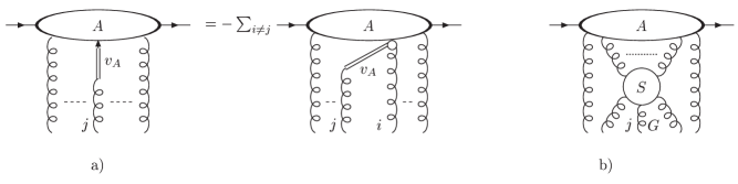
The $K$ gluon carries scalar polarization. Since the jet $A$ function has no internal tulip-garden subtractions (they are contained in the soft function $S$), we can use the Ward identities of the theory [34], which are readily derived from its underlying BRS symmetry [35], to decouple this gluon from the rest of the jet $A$ after we sum over all possible insertions of the gluon. The result is

$$J_{A}^{(n)\,a_{1}\ldots\,a_{j}\ldots\,a_{n}}(p_{A},q,v_{B},\eta;k_{1},\ldots,k_{i},\ldots,k_{j},\ldots,k_{n}) = -\frac{1}{v_{A}\cdot k_{j}-i\epsilon}\sum^{n}_{i\neq j}\left(-ig_{s}f^{c_{i}a_{i}a_{j}}\right)$$

$$\times\,J_{A}^{(n-1)\,a_{1}\ldots\,c_{i}\ldots\,{\underline{a}}_{j}\,\ldots\,a_{n}}(p_{A},q,v_{B},\eta;k_{1},\ldots,k_{i}+k_{j},\ldots,{\underline{k}}_{j},\ldots k_{n}).$$

The notation ${\underline{a}}_{j}$ and ${\underline{k}}_{j}$ indicates that the jet function $J_{A}^{(n-1)}$ does not depend on the color index $a_{j}$ and the momentum $k_{j}$, because they have been factored out. In Eq. (4.1), $g_{s}$ is the QCD coupling constant and $f^{c_{i}a_{i}a_{j}}$ are the structure constants of the $SU(3)$ algebra. The pictorial representation of this equation is shown in Fig. 3a. The arrow represents a scalar polarization and the double line stands for the eikonal line. The Feynman rules for the special vertices and the eikonal lines in Fig. 3a are listed in Appendix D. Strictly speaking the right-hand side of Eq. (4.1) and Fig. 3a contain contributions involving external ghost lines. However, from the power counting arguments of Sec. 3.2 we know that when all lines inside of the jet are jet-like, the jet function can contain neither external nor internal ghost lines. Therefore Eq. (4.1) is valid up to power suppressed corrections for this momentum configuration.

The idea behind the $K$-$G$ decomposition is that the contribution of the soft $G$ gluon attached to the jet line in the leading power is proportional to $v_{B}^{\mu}G_{\mu\nu}v_{A}^{\nu}=0$. In order to avoid this suppression, the $G$ gluon must be attached to a soft line. The general reduced diagram corresponding to the $G$ gluon attached to jet $A$ is depicted in Fig. 3b. The lines coming out of $S$ as well as the lines included in it are soft. The letter $G$ next to the $j$th gluon in Fig. 3b reminds us that this gluon is a $G$-gluon attaching to jet $J_{(A)\,\mu}$ via the $G^{+\mu}(k_{j})$ vertex.

The reasoning described above applies to the case when all components of soft momenta are of the same order. In the situation of Coulomb (Glauber) momenta, this picture is not valid anymore, since the large ratio $k_{\perp}/k^{-}$ coming from the $G^{+\perp}$ component can compensate for the suppression due to the attachment of the $G$ part to a jet $A$ line via the transverse components of the vertex.

4.2 Variation of a jet function with respect to a gauge fixing vector $\eta$

In this subsection we find the variation of the jet function $J_{A}^{(n)}$ with respect to a gauge fixing vector $\eta$. The motivation to do this can be easily understood. We consider the jet function with one soft gluon attached to it only, $J_{A}^{(1)}(p_{A},q,v_{B},\eta)$. Let us define

$${\xi}_{A}\equiv p_{A}\cdot\eta\;\;\mbox{and}\;\;{\zeta}_{B}\equiv\eta\cdot v_{B}.$$ (31)

In these terms, jet function $J_{A}^{(1)}$ can depend on the following kinematical combinations:
$J_{A}^{(1)}(p_{A},q,v_{B},\eta)=J_{A}^{(1)}({\xi}_{A},\,p_{A}\cdot v_{B},\,{\zeta}_{B},\,t)$. Using the identity $p_{A}\cdot v_{B}=2\,{\xi}_{A}{\zeta}_{B}$ and the fact, that the dependence of $J_{A}$ on the vector $v_{B}$ is introduced trivially via Eq. (3.3), we conclude that

$$J_{A}^{(1)}(p_{A},q,v_{B},\eta)={\zeta}_{B}\,{\bar{J}}_{A}^{(1)}({\xi}_{A},\,t).$$ (32)

Our aim is to resum the large logarithms of $\ln(p_{A}^{+})$ that appear in the perturbative expansion of the jet $A$ function. In order to do so, we shall derive an evolution equation for $p_{A}^{+}\,\partial J^{(1)}_{A}/\partial p_{A}^{+}$. Since $p_{A}$ appears in combination with $\eta$ only, we can trace out the $p_{A}^{+}$ dependence of $J_{A}^{(1)}$ by tracing out its dependence on $\eta$. This can be achieved by varying the gauge fixing vector $\eta$. The idea goes back to Collins and Soper [32] and Sen [31]. We will generalize the result to $J_{A}^{(n)}$ in Sec. 5.2.

We consider a variation that corresponds to an infinitesimal Lorentz boost in a positive $+$ direction with velocity $\delta\beta$. Thus, for the gauge fixing vector $\eta=(1,0,0,0)$ , Eq. (9), the variation is: $\delta\eta\equiv{\tilde{\eta}}\,\delta\beta\equiv(0,0,0,1)\,\delta\beta$. It leaves invariant the norm ${\eta}^{2}=1$ to order ${\cal O}(\delta\beta)$. The precise relation between the variation of the jet $A$ function with respect to $p_{A}^{+}$ and $\delta{\eta}^{\alpha}$ is

$$p_{A}^{+}\frac{\partial J_{A}^{(1)}}{\partial\,p_{A}^{+}}=-{\tilde{\eta}}^{\alpha}\frac{\partial J_{A}^{(1)}}{\partial\,\eta^{\alpha}}+{\zeta}_{B}\frac{\partial J_{A}^{(1)}}{\partial{\zeta}_{B}}=-{\tilde{\eta}}^{\alpha}\frac{\partial J_{A}^{(1)}}{\partial\,\eta^{\alpha}}+J_{A}^{(1)}.$$ (33)

We have used the chain rule in the first equality and the simple relation ${\zeta}_{B}\,\partial J_{A}^{(1)}/\partial{\zeta}_{B}=J_{A}^{(1)}$, following from Eq. (32), in the second one.

Figure 4: The result of a variation of jet function $J_{A}^{(n)}$ with respect to a gauge fixing vector.

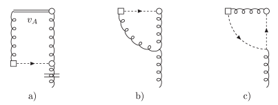
In order for Eq. (33) to be useful, we need to know what the variation of jet $A$ with respect to the gauge fixing vector $\eta$ is. The result of this variation for $J_{A}^{(n)}$ is shown in Fig. 4. It can be derived using either the formalism of the effective action, Ref. [36], or a diagrammatic approach first suggested in Ref. [32] and performed in axial gauge. We give an argument how Fig. 4 arises in Appendix B. Here we only note that the form of the diagrams in Fig. 4 is a direct consequence of a 1PI nature of the jet functions. The explicit form of the boxed vertex

$$-i\,S^{\alpha}(k)\equiv-i\left(\eta\cdot k\,{\tilde{\eta}}^{\alpha}+{\tilde{\eta}}\cdot k\,\eta^{\alpha}\right),$$ (34)

as well as of the circled vertex is given in Fig. 13 of Appendix D, while their origin is demonstrated in Appendix B. The dashed lines in Fig. 4 represent ghosts, and these are also given in Fig. 13 of Appendix D. The four vectors $\eta$, given in Eq. (9), and

$${\tilde{\eta}} = \left(\frac{1}{\sqrt{2}},-\frac{1}{\sqrt{2}},0_{\perp}\right),$$ (35)

appearing in Eq. (34) are defined in the partonic c.m. frame, Eq. (2). We list the components of $S_{\mu}\,N^{\mu\,\alpha}(k)$

$$S_{\mu}(k)\,N^{\mu\,\pm}(k) = k^{\mp}\left(\frac{k_{+}^{2}-k_{-}^{2}}{2\,k\cdot\bar{k}}\pm 1\right),$$

$$S_{\mu}(k)\,N^{\mu\,i}(k) = \frac{k_{-}^{2}-k_{+}^{2}}{2k\cdot\bar{k}}\,k^{i},$$ (36)

for later reference.

In Fig. 4, we sum over all external gluons. This is indicated by the sum over $i$. In addition, we sum over all possible insertions of external soft gluons $\{i_{1},\ldots,i_{n_{\pi}}\}\in\{1,\ldots,n\}\backslash\{i\}$. This summation is denoted by the symbol $\pi$. We note that at lowest order, with only a gluon $i$ attached to the vertical blob in Fig. 4b, this vertical blob denotes the transverse tensor structure depending on the momentum $k_{i}$ of this gluon

$$i\left(k_{i}^{2}g^{\alpha\beta}-k_{i}^{\alpha}k_{i}^{\beta}\right).$$ (37)

It is labeled by a gluon line which is crossed by two vertical lines, Fig. 13. The ghost line connecting the boxed and the circled vertices in Fig. 4b can interact with jet $A$ via the exchange of an arbitrary number of soft gluons. We do not show this possibility in Fig. 4b for brevity.

Let us now examine what the important integration regions for a loop with momentum $k$ in Fig. 4b are. The presence of the ghost line and of the nonlocal boxed vertex requires that in the leading power the loop momentum $k$ must be soft. It can be neither collinear nor hard. This will enable us to factor the gluon with momentum $k$ from the rest of the jet according to the procedure described in Sec. 4.1.

4.3 Dependence of a jet function on the plus component of a soft gluon’s momentum attached to it

In this subsection we want to find the leading regions of the object $k_{j}^{+}{\partial J_{A}^{(n)}}/{\partial}k_{j}^{+}$. This information will be essential for the analysis pursued in the next sections. For a given diagram contributing to $J_{A}^{(n)}$ we can always label the internal loop momenta in such a way that the momentum $k_{j}$ flows along a continuous path connecting the vertices where the momentum $k_{j}$ enters and leaves the jet function $J_{A}^{(n)}$. When we apply the operation $k_{j}^{+}\partial/\partial k_{j}^{+}$ on a particular graph corresponding to $J_{A}^{(n)}$, it only acts on the lines and vertices which form this path. The idea is illustrated in Fig. 5a. The gluon with momentum $k$ attaches to jet $A$ via the three-point vertex $v_{1}$. Then the momentum $k$ flows through the path containing the vertices $v_{1},v_{2},v_{3}$ and the lines $l_{1},l_{2}$. The action of the operator $k^{+}\partial/\partial k^{+}$ on a line or vertex which carries jet-like momentum gives a negligible contribution, since the $+$ component of this lines momentum will be insensitive to $k^{+}$. In order to get a non-negligible contribution, the corresponding line must be soft. In Fig. 5a, lines $l_{1}$ and $l_{2}$ must be soft in order to get a non-suppressed contribution from the diagram after we apply the $k^{+}\partial/\partial k^{+}$ operation on it. This, with the fact that the external soft gluons carry soft momenta, also implies that the lines $l_{3},\ldots,\,l_{6}$ must be soft. This reasoning suggests that in general a typical contribution to $k_{j}^{+}{\partial J_{A}^{(n)}}/{\partial}k_{j}^{+}$ comes from the configurations shown in Fig. 5b. It can be represented as

$$J_{A}^{(n)\,a_{1}\,\ldots\,a_{n}} = \int\left(\prod_{i=1}^{n^{\prime}-1}{\mathrm{d}}^{D}k^{\prime}_{i}\right)\,\,j^{(n,n^{\prime})\,a_{1}\,\ldots\,a_{n},\,a^{\prime}_{1}\,\ldots\,a^{\prime}_{n^{\prime}}}(v_{A},q,\eta;k_{1},\ldots,k_{n};k^{\prime}_{1},\ldots,k^{\prime}_{n^{\prime}})$$ (38)

$$\times J_{A}^{(n^{\prime})\,a^{\prime}_{1}\,\ldots\,a^{\prime}_{n^{\prime}}}(p_{A},q,\eta,v_{B};k^{\prime}_{1},\ldots,k^{\prime}_{n^{\prime}}).$$

Figure 5: a) Momentum flow of the external soft gluon inside of jet $A$. b) Typical contribution to $k_{j}^{+}{\partial J_{A}^{(n)}}/{\partial}k_{j}^{+}$.

The function $j^{(n,n^{\prime})}$ contains the contributions from the soft part $S$ and from the gluons connecting the jet $J_{A}^{(n^{\prime})}$ and $S$ in Fig. 5b. The jet function $J_{A}^{(n^{\prime})}$ has fewer loops than the original jet function $J_{A}^{(n)}$. Now applying the operation $k_{j}^{+}{\partial}/{\partial}k_{j}^{+}$ to Eq. (38), the operator $k_{j}^{+}{\partial}/{\partial}k_{j}^{+}$ acts only to the function $j^{(n,n^{\prime})}$. Hence we can write

$$k_{j}^{+}\frac{\partial}{k_{j}^{+}}J_{A}^{(n)\,a_{1}\,\ldots\,a_{n}} = \int\left(\prod_{i=1}^{n^{\prime}-1}{\mathrm{d}}^{D}k^{\prime}_{i}\right)k_{j}^{+}\frac{\partial}{\partial k_{j}^{+}}\,j^{(n,n^{\prime})\,a_{1}\,\ldots\,a_{n},\,a^{\prime}_{1}\,\ldots\,a^{\prime}_{n^{\prime}}}(v_{A},q,\eta;k_{1},\ldots,k_{n};k^{\prime}_{1},\ldots,k^{\prime}_{n^{\prime}})$$ (39)

$$\times J_{A}^{(n^{\prime})\,a^{\prime}_{1}\,\ldots\,a^{\prime}_{n^{\prime}}}(p_{A},q,\eta,v_{B};k^{\prime}_{1},\ldots,k^{\prime}_{n^{\prime}}).$$

We conclude that the contribution to $k_{j}^{+}{\partial J_{A}^{(n)}}/{\partial}k_{j}^{+}$ can be expressed in terms of jet functions $J_{A}^{(n^{\prime})}$ which have fewer loops than the original jet function.

5 Factorization and Evolution Equations

We are now ready to obtain evolution equations which will enable us to resum the large logarithms. First, in Sec. 5.1, we will put Eq. (27) into what we call the second factorized form. Then, in Sec. 5.2, we derive the desired evolution equations. In Sec. 5.3, we will show the cancellation of the double logarithms and finally in Sec. 5.4, we demonstrate that the evolution equations derived in Sec. 5.2 are sufficient to determine the high-energy behavior of the scattering amplitude.

5.1 Second factorized form

The goal of this subsection is to rewrite Eq. (27) into the following form [4]

$$A = \sum_{n,m}\int\left(\prod_{i=1}^{n-1}\mathrm{d}^{D-2}k_{i\perp}\right)\left(\prod_{j=1}^{m-1}\mathrm{d}^{D-2}p_{j\perp}\right)\,{\Gamma}_{A}^{(n)\,a_{1}\ldots\,a_{n}}(p_{A},q,\eta,v_{B};k_{1\perp},\ldots,k_{n\perp};M)$$ (40)

$$\times S^{{}^{\prime}\,(n,m)}_{a_{1}\ldots\,a_{n},\,b_{1}\ldots\,b_{m}}(q,\eta,v_{A},v_{B};k_{1\perp},\ldots,k_{n\perp};p_{1\perp},\ldots,p_{m\perp};M)$$

$$\times {\Gamma}_{B}^{(m)\,b_{1}\ldots\,b_{m}}(p_{B},q,\eta,v_{A};p_{1\perp},\ldots,p_{m\perp};M),$$

where ${\Gamma}_{A}^{(n)}$ and ${\Gamma}_{B}^{(m)}$ are defined as the integrals of the jet functions $J_{A}^{(n)}$ and $J_{B}^{(m)}$, over the minus and plus components, respectively, of their external soft momenta, with the remaining light-cone components of soft momenta set to zero,

$${\Gamma}_{A}^{(n)\,a_{1}\ldots\,a_{n}}(p_{A},q,\eta,v_{B};k_{1\perp},\ldots,k_{n\perp};M) \equiv \prod_{i=1}^{n-1}\left(\int_{-M}^{M}\mathrm{d}k^{-}_{i}\right)\,J_{A}^{(n)\,a_{1}\ldots\,a_{n}}(p_{A},q,\eta,v_{B};k_{1\perp},\ldots,k_{n\perp},$$

$$k_{1}^{+}=0,\ldots,k_{n}^{+}=0,k_{1}^{-},\ldots,k_{n}^{-}),$$

$${\Gamma}_{B}^{(m)\,b_{1}\ldots\,b_{m}}(p_{B},q,\eta,v_{A};p_{1\perp},\ldots,p_{m\perp};M) \equiv \prod_{i=1}^{m-1}\left(\int_{-M}^{M}\mathrm{d}p^{+}_{i}\right)\,J_{B}^{(m)\,b_{1}\ldots\,b_{m}}(p_{B},q,\eta,v_{A};p_{1\perp},\ldots,p_{m\perp},$$ (41)

$$p_{1}^{-}=0,\ldots,p_{m}^{-}=0,p_{1}^{+},\ldots,p_{m}^{+}).$$

In Eq. (40), $S^{\prime}$ is a calculable function of its arguments and $M$ is an arbitrary scale of the order $\sqrt{|t|}$. The functions ${\Gamma}_{A,B}$ and $S^{\prime}$ depend individually on this scale, but the final result, of course, does not. Based on the discussion at the end of Sec. 3.3, one can immediately recognize that all the large logarithms are now contained in the functions ${\Gamma}_{A}$ and ${\Gamma}_{B}$. The convolution of ${\Gamma}_{A},{\Gamma}_{B}$ and $S^{\prime}$ is over the transverse momenta of the exchanged soft gluons. Since these momenta are restricted to be of the order $\sqrt{|t|}$, the integration over transverse momenta cannot introduce $\ln(s/|t|)$. This indicates that at leading logarithm approximation the factorized diagram with the exchange of one gluon only contributes. In general, when we consider a contribution to the amplitude at $L=L_{A}+L_{B}+L_{S^{\prime}}$ loop level, where $L_{A},L_{B}$ and $L_{S^{\prime}}$ is the number of loops in ${\Gamma}_{A},{\Gamma}_{B}$ and $S^{\prime}$, respectively, we can get $L-L_{S^{\prime}}$ logarithms of $s/|t|$ at most. Hence, the investigation of the $s/t$ dependence of the full amplitude reduces to the study of the $p_{A}^{+}$ and $p_{B}^{-}$ dependence of ${\Gamma}_{A}$ and ${\Gamma}_{B}$, respectively. We formalize this statement at the end of Sec. 5.3 after we have proved that $\Gamma_{A}$ ($\Gamma_{B}$) contains one logarithm of $p_{A}^{+}$ ($p_{B}^{-}$) per loop.

Let us now show how we can systematically go from Eq. (27) to Eq. (40). We follow the method developed in Ref. [4]. We start from Eq. (27) and consider the $k_{i}^{-}$ integrals over the jet function $J_{A}$ for fixed $k^{+}_{i},\,k_{i\perp}$:

$$A=\sum_{n}\int\prod_{i=1}^{n-1}{\mathrm{d}}k_{i}^{-}\;R_{A}^{\,a_{1}\ldots\,a_{n}}(k_{1}^{-},\ldots,k_{n}^{-};\ldots)\,J_{A}^{(n)\,a_{1}\ldots\,a_{n}}(p_{A},q,\eta,v_{B};k_{1},\ldots,k_{n}),$$ (42)

where $R_{A}$ is given by the soft function $S$ and the jet function $J_{B}$,

$$R_{A}^{\,a_{1}\ldots\,a_{n}}(k_{1}^{-},\ldots,k_{n}^{-};\ldots) = \sum_{m}\int\left(\prod^{m-1}_{j=1}\mathrm{d}^{D}p_{j}\right)\,S^{(n,m)}_{a_{1}\ldots\,a_{n},b_{1}\ldots\,b_{m}}(q,\eta,v_{A},v_{B};k_{1},\ldots,k_{n};p_{1},\ldots,p_{m})$$ (43)

$$\times J_{B}^{(m)\,b_{1}\ldots\,b_{m}}(p_{B},q,\eta,v_{A};p_{1},\ldots,p_{m}).$$

We next use the following identity for $R_{A}$:

$$R_{A}(k_{1}^{-},\ldots,k_{n-1}^{-}) = R_{A}(k_{1}^{-}=0,\ldots,k_{n-1}^{-}=0)\,\prod_{i=1}^{n-1}{\theta}(M-|k_{i}^{-}|)$$ (44)

$$+ \sum^{n-1}_{i=1}\;\left[R_{A}(k_{1}^{-},\ldots,k_{i}^{-},k_{i+1}^{-}=0,\ldots,k_{n-1}^{-}=0)\right.$$

$$- \left.R_{A}(k_{1}^{-},\ldots,k_{i-1}^{-},k_{i}^{-}=0,\ldots,k_{n-1}^{-}=0)\,{\theta}(M-|k_{i}^{-}|)\right]$$

$$\times \prod_{j=i+1}^{n-1}{\theta}(M-|k_{j}^{-}|).$$

We have suppressed the dependence on the color indices and other possible arguments in $R_{A}$ for brevity. The scale $M$ can be arbitrary, but, as above, we take it to be of the order of $\sqrt{|t|}$. The first term on the right hand side of Eq. (44) has all $k_{i}^{-}=0$. The rest of the terms can be analyzed using the $K$-$G$ decomposition discussed in Sec. 4.1. Consider the ($i=1$) term, say, in the square bracket of Eq. (44) inserted in Eq. (42). Let us denote it $A_{1}$. In the region $|k_{1}^{-}|\ll M$ the integrand vanishes. On the other hand, for $|k_{1}^{-}|\sim M$ we can use the $K$-$G$ decomposition for the gluon with momentum $k_{1}$. The contribution from the $K$ part factorizes and the integral over the component $k_{1}^{-}$ has the form

$$A_{1} = \int\frac{{\mathrm{d}}k_{1}^{-}}{v_{A}\cdot k_{1}}\,\left[R_{A}^{\,a_{1}\ldots\,a_{n}}(k_{1}^{-},k_{2}^{-}=0,\ldots,k_{n-1}^{-}=0)\,-\,\theta(M-|k_{1}^{-}|)\,R_{A}^{\,a_{1}\ldots\,a_{n}}(k_{1}^{-}=0,\ldots,k_{n-1}^{-}=0)\right]$$ (45)

$$\times \sum_{i=2}^{n-1}\left(ig_{s}f^{a_{1}c_{i}a_{i}}\,\int_{-M}^{M}\prod_{j=2}^{n-1}{\mathrm{d}}k^{-}_{j}\,J_{A}^{(n-1)\,a_{2}\ldots\,c_{i}\ldots\,a_{n}}(p_{A},q,\eta,v_{B};k_{2},\ldots,k_{1}+k_{i},\ldots,k_{n})\right).$$

Eq. (45) is valid when all the lines inside the jet are jet-like. In that case the contributions from the ghosts are power suppressed. The contribution corresponding to a $G$ gluon comes from the region of integration shown in Fig. 3b. It can be expressed in the form of Eq. (42) involving some $J_{A}^{(n^{\prime})}$ with fewer loops than in the original $J_{A}^{(n)}$, and an $R_{A}^{\prime}$ with more loops than in the original $R_{A}$. Then we can repeat the steps described above with this new integral.

Every subsequent term in the square bracket of Eq. (44) can be treated the same way as the first term. This allows us to express the integral in Eq. (42) in terms of $k_{i}^{-}$ integrals over some $J_{A}^{(n^{\prime})}$s, which have the same or fewer number of loops than the original $J_{A}^{(n)}$,

$${\Gamma}_{A}^{(n^{\prime})\,a^{\prime}_{1}\ldots\,a^{\prime}_{n^{\prime}}}\left(p_{A},q,\eta,v_{B};\,k_{1}^{{}^{\prime}\;+},\ldots,k_{n^{\prime}}^{{}^{\prime}\;+};\,k^{\prime}_{1\perp},\ldots,k^{\prime}_{n^{\prime}\perp};M\right)\equiv$$

$$\int_{-M}^{M}\prod_{i=1}^{n^{\prime}-1}{\mathrm{d}}k^{{}^{\prime}\;-}_{i}\,J_{A}^{(n^{\prime})\,a^{\prime}_{1}\ldots\,a^{\prime}_{n^{\prime}}}\left(p_{A},q,\eta,v_{B};k^{\prime}_{1},\ldots,k^{\prime}_{n^{\prime}}\right).$$ (46)

We now want to set $k_{i}^{{}^{\prime}\;+}=0$ in order to put Eq. (42) into the form of Eq. (40). To that end, we employ an identity for $J_{A}^{(n^{\prime})}$ (we again suppress the dependence on the color indices for brevity)

$$J_{A}^{(n^{\prime})}(p_{A},q,\eta,v_{B};k^{\prime}_{1},\ldots,k^{\prime}_{n^{\prime}}) = J_{A}^{(n^{\prime})}\left(p_{A},q,\eta,v_{B};k_{1}^{{}^{\prime}\;+}=0,\ldots,k_{n^{\prime}}^{{}^{\prime}\;+}=0,k_{1}^{{}^{\prime}\;-},\ldots,k_{n^{\prime}}^{{}^{\prime}\;-},k^{\prime}_{1\perp},\ldots,k^{\prime}_{n^{\prime}\perp}\right)$$ (47)

$$+ \sum_{i=1}^{n^{\prime}-1}\int_{0}^{k_{i}^{{}^{\prime}\;+}}{\mathrm{d}}l^{+}_{i}\frac{\partial}{\partial l^{+}_{i}}\,J_{A}^{(n^{\prime})}\left(p_{A},q,\eta,v_{B};k^{\prime}_{1\perp},\ldots,k^{\prime}_{n^{\prime}\perp},k_{1}^{{}^{\prime}\;-},\ldots,k_{n^{\prime}}^{{}^{\prime}\;-},\right.$$

$$\left.k_{1}^{{}^{\prime}\;+},\ldots,k^{{}^{\prime}\;+}_{i-1},\,l_{i}^{+},k_{i+1}^{{}^{\prime}\;+}=0,\ldots,k_{n^{\prime}}^{{}^{\prime}\;+}=0\right).$$

Substituting the first term of Eq. (47) into Eq. (5.1), we recognize the definition for ${\Gamma}_{A}$, Eq. (5.1). We have shown in Sec. 4.3 that the contributions from the terms proportional to $\partial J_{A}^{(n^{\prime})}/\partial l^{+}_{i}$ in Eq. (47) can be expressed as soft-loop integrals of some $J_{A}^{(n^{\prime\prime})}$, again with fewer loops than in $J_{A}^{(n^{\prime})}$. When we substitute this into Eq. (5.1) we may express the resulting contribution in terms of integrals which have the form of Eq. (42). We can now repeat all the steps mentioned so far, with this new integral. By this iterative procedure we can transfer the $k_{i}^{-}$ integrals in Eq. (42) to $J_{A}^{(n)}$ and also set $k_{i}^{+}=0$ inside $J_{A}^{(n)}$. In a similar manner, we can analyze the $p_{j}^{+}$ integrals in Eq. (27), and express them in terms of ${\Gamma}_{B}$ defined in Eq. (5.1). This algorithm, indeed, leads from the first factorized form of the considered amplitude, Eq. (27), to the second factorized form, Eq. (40).

5.2 Evolution equation

We have now collected all the ingredients necessary to derive the evolution equations for quantities defined in Eq. (5.1). Consider ${\Gamma}_{A}^{(n)}$. We aim to find an expression for $p_{A}^{+}\partial{\Gamma}^{(n)}_{A}/\partial p_{A}^{+}$. As discussed in Sec. 4.2 this will enable us to resum the large logarithms of $\ln(p_{A}^{+})$ and eventually the logarithms of $\ln(s/|t|)$. According to Eq. (5.1), in order to find $p_{A}^{+}\partial{\Gamma}^{(n)}_{A}/\partial p_{A}^{+}$, we need to study $p_{A}^{+}\partial J^{(n)}_{A}/\partial p_{A}^{+}$. Using the identities $p_{A}\cdot v_{B}=2\,{\xi}_{A}{\zeta}_{B}$, $p_{A}\cdot k_{i}=2\,{\xi}_{A}{\xi}_{i}$, where ${\xi}_{i}\equiv k_{i}^{-}{\eta}^{+}$ and ${\xi}_{A},{\zeta}_{B}$ are defined in Eq. (31), we conclude that

$$J_{A}^{(n)}={\zeta}_{B}^{n}\,{\bar{J}}_{A}^{(n)}\left({\xi}_{A},\,\{{\xi}_{i}\}_{i=1}^{n-1},\,t,\,\{q_{\perp}\cdot k_{i\perp}\}_{i=1}^{n-1},\,\{k_{i\perp}\cdot k_{j\perp}\}_{i,j=1}^{n-1}\right).$$ (48)

From this structure, using the chain rule, we derive the following relation satisfied by $J_{A}^{(n)}$, which generalizes Eq. (33) to $J^{(n)}_{A}$ with arbitrary number of external gluons,

$$p_{A}^{+}\frac{\partial J_{A}^{(n)}}{\partial\,p_{A}^{+}}=-{\tilde{\eta}}^{\alpha}\frac{\partial J_{A}^{(n)}}{\partial\,{\eta}^{\alpha}}+\sum_{i=1}^{n-1}k_{i}^{-}\frac{\partial J_{A}^{(n)}}{\partial k_{i}^{-}}+{\zeta}_{B}\frac{\partial J_{A}^{(n)}}{\partial{\zeta}_{B}}.$$ (49)

Now, we integrate both sides of Eq. (49) over $\prod_{j=1}^{n-1}\left(\int_{-M}^{M}\mathrm{d}k^{-}_{j}\right)$ and set all $k_{j}^{+}=0$. Then, using the definition for ${\Gamma}_{A}^{(n)}$, Eq. (5.1), the left hand side is nothing else but $p_{A}^{+}\partial{\Gamma}^{(n)}_{A}/\partial p_{A}^{+}$. The first term on the right hand side of Eq. (49) is simply $-{\tilde{\eta}}^{\alpha}\partial\,{\Gamma}_{A}^{(n)}/\partial\,{\eta}^{\alpha}$. Noting that ${\zeta}_{B}\partial J_{A}^{(n)}/\partial{\zeta}_{B}=n\,J_{A}^{(n)}$, the last term gives simply $n\,{\Gamma}_{A}^{(n)}$. For the middle term, we use integration by parts

$$\prod_{j=1}^{n-1}\left(\int_{-M}^{M}\mathrm{d}k^{-}_{j}\right)\sum_{i=1}^{n-1}\,k_{i}^{-}\frac{\partial J_{A}^{(n)}}{\partial k_{i}^{-}}\,=\,\prod_{j=1}^{n-1}\left(\int_{-M}^{M}\mathrm{d}k^{-}_{j}\right)\sum_{i=1}^{n-1}\left[\frac{\partial}{\partial k_{i}^{-}}(k_{i}^{-}\,J_{A}^{(n)})-J_{A}^{(n)}\right]=$$ (50)

$$\sum_{i=1}^{n-1}\int_{-M}^{M}\left(\prod_{j\neq i}^{n-1}{\mathrm{d}}k_{j}^{-}\right)\,M\,\left[\,J_{A}^{(n)}(k_{i}^{-}=+M,\ldots)+J_{A}^{(n)}(k_{i}^{-}=-M,\ldots)\,\right]\;-\;(n-1)\,{\Gamma}_{A}^{(n)}.$$

Combining the partial results, Eqs. (49) and (50), we obtain the following evolution equation

$$p_{A}^{+}\,\frac{\partial\,{\Gamma}_{A}^{(n)}}{\partial\,p_{A}^{+}} = \sum_{i=1}^{n-1}\int_{-M}^{M}\left(\prod_{j\neq i}^{n-1}{\mathrm{d}}k_{j}^{-}\right)\,M\,\left[J_{A}^{(n)}(k_{i}^{-}=+M,\ldots)+J_{A}^{(n)}(k_{i}^{-}=-M,\ldots)\right]$$ (51)

$$+\,{\Gamma}_{A}^{(n)}\,-\,{\tilde{\eta}}^{\alpha}\frac{\partial\,{\Gamma}_{A}^{(n)}}{\partial\,{\eta}^{\alpha}}.$$

The jet function $J_{A}^{(n)}$ in the first term of Eq. (51) is evaluated at $\{k_{i}^{+}=0\}_{i=1}^{n}$ and the $k_{j}^{-}$s are integrated over for $j=1,\ldots,n-1$ and $j\neq i$. The first term in Eq. (51) can be analyzed using the $K$-$G$ decomposition for gluon $i$ since the $k_{i}^{-}$ is evaluated at the scale $M\sim\sqrt{|t|}$. The outcome of the last term in Eq. (51) has been determined in Sec. 4.2, Fig. 4 . As a result we have all the tools necessary to determine the asymptotic behavior of the high energy amplitude for process (1). To demonstrate this, we will rewrite Eq. (51) into the form where on the right hand side there will be a sum of terms involving ${\Gamma}_{A}^{(n^{\prime})}$s convoluted with functions which do not depend on $p_{A}^{+}$. Let us proceed term by term.

Again, the $K$-$G$ decomposition applies to the first term in Eq. (51) because the external momenta are fixed with $k_{i}^{-}=\pm M$. Using the factorization of a $K$ gluon given in Eq. (4.1) it is clear that the contributions from the $K$ gluons cancel for $J_{A}^{(n)}$s evaluated at $k_{i}^{-}=+M$ and $k_{i}^{-}=-M$. Hence only the $G$ gluon contribution survives in this term. Its most general form is shown in Fig. 3b. Before writing it down let us introduce the following notation. For a set of indices $\{1,2,\ldots,n\}\backslash\{i\}$ consider all the possible subsets of this set, with $1,2,\ldots,(n-1)$ number of elements. Let us denote a given subset by $\pi$, its complementary subset $\bar{\pi}$, the number of elements in this subset as $n_{\pi}$ and in its complementary as $n_{\bar{\pi}}\equiv(n-1)-n_{\pi}$. With this notation, we can write the $i$th contribution to the first term in Eq. (51) in the form

$$J_{A}^{(n)\,a_{1}\,\ldots\,a_{n}}\left(k_{i}^{-}=+M,\ldots\right)+J_{A}^{(n)\,a_{1}\,\ldots\,a_{n}}\left(k_{i}^{-}=-M,\ldots\right)=\sum_{\pi}\int\prod_{j=1}^{N-1}\frac{{\mathrm{d}}^{D}l_{j}}{(2\pi)^{D}}$$

$$S^{\mu_{1}\ldots\,\mu_{N}}_{a_{i}\,a_{i_{1}}\ldots\,a_{i_{n_{\pi}}}\,b_{1}\ldots\,b_{N}}\left(k_{i}^{-}=+M,k_{i_{1}}^{-},\ldots,k_{i_{n_{\pi}}}^{-};k_{i}^{+}=0,k_{i_{1}}^{+}=0,\ldots,k_{i_{n_{\pi}}}^{+}=0;k_{i\perp},k_{i_{1}\,\perp},\ldots,k_{i_{n_{\pi}}\,\perp};\right.$$

$$\left.l_{1},\ldots,l_{N};q,\eta\right)\,\times\,J_{A\;\mu_{1}\ldots\,\mu_{N}}^{(n_{\bar{\pi}}+N)\,a_{\bar{i}_{1}}\,\ldots\,a_{\bar{i}_{n_{\bar{\pi}}}}\,b_{1}\ldots\,b_{N}}\left(k_{\bar{i}_{1}}^{-},\ldots,k_{\bar{i}_{n_{\bar{\pi}}}}^{-};k_{\bar{i}_{1}}^{+}=0,\ldots,k_{\bar{i}_{n_{\bar{\pi}}}}^{+}=0;k_{\bar{i}_{1}\,\perp},\ldots,k_{\bar{i}_{n_{\bar{\pi}}}\,\perp};\right.$$

$$\left.l_{1},\ldots,l_{N};p_{A},q,\eta\right)+(k_{i}^{-}\rightarrow-M).$$ (52)

In Eq. (5.2), the summation over repeated indices is understood. We sum over all possible subsets $\pi$. In other words, we sum over all possible attachments of external gluons to jet function $J_{A}$ and to the soft function $S$. The elements of a given set $\pi$ are denoted $i_{1},i_{2},\ldots,i_{n_{\pi}}$. The elements of a complementary set $\bar{\pi}$ are labeled $\bar{i}_{1},\bar{i}_{2},\ldots,\bar{i}_{n_{\bar{\pi}}}$. The number of gluons connecting $S$ and $J_{A}^{(n_{\bar{\pi}}+N)}$ is $N$.

Following the procedure described in Sec. 5.1 with $R_{A}$ in Eq. (42) replaced by $S$ in Eq. (5.2), we can express the contribution from a $G$ gluon in the first term of Eq. (51) in a form

$$\sum_{i=1}^{n-1}\int_{-M}^{M}\left(\prod_{j\neq i}^{n-1}{\mathrm{d}}k_{j}^{-}\right)\,M\,\left[J_{A}^{(n)\,a_{1}\,\ldots\,a_{n}}(k_{i}^{-}=+M,\ldots)+J_{A}^{(n)\,a_{1}\,\ldots\,a_{n}}(k_{i}^{-}=-M,\ldots)\right]=$$ (53)

$$\sum_{m}\int\prod_{j=1}^{m}\,{\mathrm{d}}^{D-2}l_{j\perp}\,{\cal K}^{(n,m)}_{a_{1}\ldots\,a_{n};\,b_{1}\ldots\,b_{m}}(k_{1\perp},\ldots,k_{n\perp},l_{1\perp},\ldots,l_{m\perp};q,\eta;M)$$

$$\times \Gamma^{(m)\,b_{1}\ldots\,b_{m}}_{A}(p_{A},q,\eta;l_{1\perp},\ldots,l_{m\perp};M).$$

The function ${\cal K}^{(n,m)}$ does not contain any dependence on $p_{A}$. It can contain delta functions setting some of the color indices $b_{i}$, as well as transverse momenta $l_{i\perp}$ of $\Gamma_{A}^{(m)}$ equal to color indices $a_{i}$ and transverse momenta $k_{i\perp}$ of $\Gamma_{A}^{(n)}$.

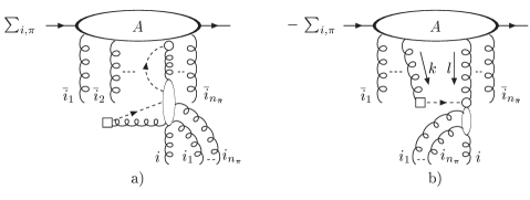
Next we turn our attention to the last term appearing in Eq. (51). The contribution to this term has been depicted graphically in Fig. 4. Consider the term in Fig. 4a. It can be written in a form

$$\int_{-M}^{M}\left(\prod_{j=1}^{n-1}{\mathrm{d}}\,k_{j}^{-}\right)\,\left(\mathrm{Fig}.\,\ref{variationJ}\mathrm{a}\right)=\int_{-M}^{M}\left(\prod_{j=1}^{n-1}{\mathrm{d}}\,k_{j}^{-}\right)\sum_{{\pi}}S^{\prime}_{a_{i}\,a_{i_{1}}\ldots\,a_{i_{n_{\pi}}}\,b}\,(k_{i}^{-},k_{i_{1}}^{-},\ldots,k_{i_{n_{\pi}}}^{-};$$

$$k_{i}^{+}=0,k_{i_{1}}^{+}=0,\ldots,k_{i_{n_{\pi}}}^{+}=0;k_{i\,\perp},k_{i_{1}\,\perp},\ldots,k_{i_{n_{\pi}}\,\perp};l=k_{i}+k_{i_{1}}+\ldots+k_{i_{n_{\pi}}};q,\eta)$$

$$\times\;J_{A}^{(n_{\bar{\pi}}+1)\,a_{\bar{i}_{1}}\,\ldots a_{\bar{i}_{n_{\bar{\pi}}}}\,b}(k_{\bar{i}_{1}}^{-},\ldots,k_{\bar{i}_{n_{\bar{\pi}}}}^{-};k_{\bar{i}_{1}}^{+}=0,\ldots,k_{\bar{i}_{n_{\bar{\pi}}}}^{+}=0;k_{\bar{i}_{1}\,\perp},\ldots,k_{\bar{i}_{n_{\bar{\pi}}}\,\perp};\,$$

$$\hskip 99.58464ptl=k_{i}+k_{i_{1}}+\ldots+k_{i_{n_{\pi}}};p_{A},q,\eta).$$ (54)

In Eq. (5.2), we have used the same notation as in Eq. (5.2). Momentum $l$ connects $S^{\prime}$ with $J_{A}^{(n_{\bar{\pi}}+1)}$. Following the same procedure as in Sec. 5.1 with $R_{A}$ appearing in Eq. (42) replaced by $S^{\prime}$ introduced in Eq. (5.2), we can express this contribution in a form given by Eq. (53) with a different kernel ${\cal K}^{(n,m)}$.

The contribution from Fig. 4b can be written

$$\int_{-M}^{M}\left(\prod_{j=1}^{n-1}{\mathrm{d}}\,k_{j}^{-}\right)\,\left(\mathrm{Fig}.\,\ref{variationJ}\mathrm{b}\right)\,=\,\int_{-M}^{M}\left(\prod_{j=1}^{n-1}{\mathrm{d}}\,k_{j}^{-}\right)\sum_{{\pi}}\int\frac{\mathrm{d}^{D}k}{(2\pi)^{D}}\,S^{\prime\prime}_{a_{i}\,a_{i_{1}}\ldots\,a_{i_{n_{\pi}}}\,b\,c}\,(k_{i}^{-},$$

$$k_{i_{1}}^{-},\ldots,k_{i_{n_{\pi}}}^{-};k_{i}^{+}=0,k_{i_{1}}^{+}=0,\ldots,k_{i_{n_{\pi}}}^{+}=0;k_{i\,\perp},k_{i_{1}\,\perp},\ldots,k_{i_{n_{\pi}}\,\perp};k,l;q,\eta)\,\times$$

$$J_{A}^{(n_{\bar{\pi}}+2)\,a_{\bar{i}_{1}}\,\ldots\,a_{\bar{i}_{n_{\bar{\pi}}}}\,b\,c}\left(k_{\bar{i}_{1}}^{-},\ldots,k_{\bar{i}_{n_{\bar{\pi}}}}^{-};k_{\bar{i}_{1}}^{+}=0,\ldots,k_{\bar{i}_{n_{\bar{\pi}}}}^{+}=0;k_{\bar{i}_{1}\,\perp},\ldots,k_{\bar{i}_{n_{\bar{\pi}}}\,\perp};k,l;p_{A},q,\eta\right).$$ (55)

The flow of momenta $k$ and $l$ is exhibited in Fig. 4b. The momentum $k$ flows through the boxed vertex and the ghost line shown in Fig. 4b which forces this momentum to be soft, so that lines $k$ and $l$ are part of the function $S^{\prime\prime}$. Since the line with momentum $k$ is soft, then all gluons attaching to $J_{A}^{(n_{\bar{\pi}}+2)}$ in Eq. (5.2) are soft and we can again apply the procedure described in Sec. 5.1 to bring the contribution in Fig. 4b into the form given by Eq. (53) with a different kernel, of course.

In summary, we have demonstrated that all the terms on the right hand side of Eq. (51) can be put into the form given by Eq. (53). This indicates that Eq. (51), indeed, describes the evolution of $\Gamma_{A}^{(n)}$ in $\ln p_{A}^{+}$ since it can be written as

$$\left(p_{A}^{+}\,\frac{\partial}{\partial\,p_{A}^{+}}-1\right)\,{\Gamma}_{A}^{(n)\;a_{1}\ldots\,a_{n}}(p_{A},q,\eta;k_{1\perp},\ldots,k_{n\perp})=$$ (56)

$$\sum_{m}\int\prod_{j=1}^{m}\,{\mathrm{d}}^{D-2}l_{j\perp}\,{\cal K}^{(n,m)}_{a_{1}\ldots\,a_{n};\,b_{1}\ldots\,b_{m}}(k_{1\perp},\ldots,k_{n\perp},l_{1\perp},\ldots,l_{m\perp};q,\eta)$$

$$\times\,\Gamma^{(m)\;b_{1}\ldots\,b_{m}}_{A}(p_{A},q,\eta;l_{1\perp},\ldots,l_{m\perp}).$$

The kernels ${\cal K}^{(n,m)}$ do not depend on $p_{A}^{+}$. As indicated above, they can contain delta functions setting some of the color indices $b_{i}$, as well as transverse momenta $l_{i\perp}$ of $\Gamma_{A}^{(m)}$ equal to color indices $a_{i}$ and transverse momenta $k_{i\perp}$ of $\Gamma_{A}^{(n)}$. The systematic use of this evolution equation enables us to resum large logarithms $\ln(p_{A}^{+})$ at arbitrary level of logarithmic accuracy. Analogous equation is satisfied by $\Gamma_{B}$. It resums logarithms of $\ln(p_{B}^{-})$.

5.3 Counting the number of logarithms

Having derived the evolution equations for ${\Gamma}_{A}^{(n)}$, Eqs. (51) and (56), it does not take too much effort to show that at $r$-loop order the amplitude contains at most $r$ powers of $\ln(s/|t|)$. We follow the method of Ref. [4]. We have argued in Sec. 5.1 that the power of $\ln(s/|t|)$ in the overall amplitude corresponds to the power of $\ln(p_{A}^{+})$ in ${\Gamma}_{A}^{(n)}$. So we have to demonstrate that at $r$-loop order ${\Gamma}_{A}^{(n,r)}$, where ${\Gamma}_{A}^{(n,r)}$ represents a contribution to ${\Gamma}_{A}^{(n)}$ at $r$-loop level, does not contain more than $r$ logarithms of $\ln(p_{A}^{+})$. We prove this statement by induction. First of all, the tree level contribution to ${\Gamma}_{A}^{(n,0)}$ is proportional to the expression

$$\int_{-M}^{M}\left(\prod_{i=1}^{n-1}{\mathrm{d}}k_{i}^{-}\right)\sum_{\{i_{1},\ldots,i_{n}\}}\,\prod_{j=1}^{n-1}\,\frac{1}{(p_{A}-\sum_{l=1}^{j}k_{i_{l}})^{2}+i\epsilon}\,\left(\prod_{j=n}^{1}\,t^{a_{i_{j}}}\right)_{r_{1},r_{A}},$$ (57)

where $t^{a_{i_{j}}}$s are the generators of the $SU(3)$ algebra in the fundamental representation. The sum over $\{i_{1},\ldots,i_{n}\}$ indicates that we sum over all possible insertions of the external soft gluons. Eq. (57) is evaluated at $\{k_{i}^{+}=0\}_{i=1}^{n}$. Expanding the denominators in Eq. (57) we obtain the expression $-2p_{A}^{+}(k_{i_{1}}^{-}+\ldots+k_{i_{j}}^{-})-(k_{i_{1}}+\ldots+k_{i_{j}})^{2}_{\perp}+i\epsilon$. We see that the poles in $k_{i}^{-}$ planes are not pinched and therefore the $k_{i}^{-}$ integrals cannot produce $\ln(p_{A}^{+})$ enhancements.

Next we assume that the statement is true at $r$-loop order, and show that it then also holds at $(r+1)$-loop level. To this end we consider the evolution equation, Eq. (51), and examine $(p_{A}^{+}\,\partial/\partial\,p_{A}^{+}-1)\,{\Gamma}_{A}^{(n,r+1)}$. Its contribution is given by the first and the third term on the right hand side of Eq. (51). As already mentioned, the first term in Eq. (51) can be analyzed using $K$-$G$ decomposition. The contributions from the $K$ terms cancel each other while the contribution from the $G$ gluons are given by the kind of diagram shown in Fig. 3b. The latter, however, can be written as a sum of soft loop integrals over $J_{A}^{(n^{\prime},r^{\prime})}$ with $r^{\prime}\leq r$, since we loose at least one loop in the original $J_{A}^{(n,r+1)}$ due to the soft momentum integration. This is demonstrated in Eq. (5.2). Following the procedure described in Sec. 5.1, we may express these contributions as transverse momentum integrals of some ${\Gamma}_{A}^{(n^{\prime},r^{\prime})}$, see Eq. (53). These contain at most $r^{\prime}\leq r$ logarithms of $\ln(p_{A}^{+})$. The contribution from the third term in the evolution equation, Eq. (51), is given by the diagrams depicted in Fig. 4. These are again soft loop integrals of some $J_{A}^{(n^{\prime},r^{\prime})}$ with $r^{\prime}\leq r$, and they can be expressed as transverse momentum integrals of ${\Gamma}_{A}^{(n^{\prime},r^{\prime})}$, see Eqs. (5.2) and (5.2), which have, therefore, at most $r$ logarithms of $\ln(p_{A}^{+})$. Since both terms on the right hand side of Eq. (51) have at most $r$ logarithms of $\ln(p_{A}^{+})$, then also $p_{A}^{+}\partial\,{\Gamma}_{A}^{(n,r+1)}/\partial\,p_{A}^{+}$ has at most $r$ logarithms of $\ln(p_{A}^{+})$ at $(r+1)$-loop level. This immediately shows that ${\Gamma}_{A}^{(n,r+1)}$ itself cannot have more than $(r+1)$ logarithms of $\ln(p_{A}^{+})$ at $(r+1)$-loop level.

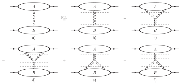
This result enables us to formally classify the types of diagrams which contribute to the amplitude at the $k$-th nonleading logarithm level. As has been shown in Sec. 5.1, we can write an arbitrary contribution to the amplitude for process (1) in the Regge limit in the second factorized form given by Eq. (40). Consider an $r$-loop contribution to the amplitude and let $L_{A}$, $L_{B}$ and $L_{S}$ be the number of loops contained in $\Gamma_{A}$, $\Gamma_{B}$ and $S$. Since $\Gamma_{A}$ ($\Gamma_{B}$) can contain $L_{A}$ ($L_{B}$) number of logarithms of $p_{A}^{+}$ ($p_{B}^{-}$) at most, the maximum number of logarithms, $N_{\mathrm{maxLog}}$, we can get is

$$N_{\mathrm{maxLog}}=r-L_{S}.$$ (58)

This indicates that when evaluating the amplitude at the $k$-th nonleading approximation, we need to consider diagrams where $1,2,\ldots,(k+1)$ soft gluons are exchanged between the jet functions $J_{A}$ and $J_{B}$.

5.4 Solution of the evolution equations

Having obtained the evolution equations, Eqs. (51) and (56), we discuss how to construct their solution. Our starting point is Eq. (56). In shorthand notation it reads

$$p_{A}^{+}\,\frac{\partial}{\partial\,p_{A}^{+}}\,{\Gamma}_{A}^{(n,r)}=\sum_{r^{\prime}=0}^{r-1}\sum_{n^{\prime}}\,{\cal K}^{(n,n^{\prime};r-r^{\prime})}\otimes\,\Gamma_{A}^{(n^{\prime},r^{\prime})},$$ (59)

at $r$-loop level. Indices $n$ and $n^{\prime}$, besides denoting the number of external gluons of the jet function, also label the transverse momenta and the color indices of these gluons. The symbol $\otimes$ in Eq. (59) denotes convolution over the transverse momenta and the color indices. Note that Eq. (59) holds for $\Gamma_{A}$ with the overall factor $p_{A}^{+}$ divided out $(\Gamma_{A}\equiv\Gamma_{A}/p_{A}^{+})$. We have proved, in Sec. 5.3, that $\Gamma_{A}^{(n,r)}$ can contain at most $r$ logarithms of $\ln(p_{A}^{+})$ at $r$-loop level. Therefore the most general expansion for $\Gamma_{A}$ is

$$\Gamma_{A}^{(n,r)}\equiv\sum_{j=0}^{r}c_{j}^{(n,r)}\,\ln^{j}(p_{A}^{+}).$$ (60)

If we want to know $\Gamma_{A}^{(n,r)}$ at ${\rm N}^{k}$LL accuracy ($k=0$ is LL, $k=1$ is NLL, etc.), we need to find all $c_{j}^{(n,r)}$ such that $r-j\leq k$. The coefficients $c_{j}^{(n,r)}$ in Eq. (60) depend on the transverse momenta and the color indices of the external gluons. Using the expansion for $\Gamma_{A}^{(n,r)}$ and $\Gamma_{A}^{(n^{\prime},r^{\prime})}$, Eq. (60), in Eq. (59) and comparing the coefficients with the same power of $\ln(p_{A}^{+})$, we obtain the recursive relation satisfied by the coefficients $c_{j}^{(n,r)}$

$$j\,c_{j}^{(n,r)}=\sum_{r^{\prime}=j-1}^{r-1}\sum_{n^{\prime}=1}^{n+r-r^{\prime}}{\cal K}^{(n,n^{\prime};r-r^{\prime})}\otimes c_{j-1}^{(n^{\prime},r^{\prime})}.$$ (61)

In Eq. (61), we have used that, in general, $1\leq n^{\prime}\leq n+r-r^{\prime}$.

We now show that Eq. (61) enables us to determine all the relevant coefficients $c_{j}^{(r,n)}$ of $\Gamma_{A}^{(n)}$ order by order in perturbation theory at arbitrary logarithmic accuracy. We start at LL, $k=0$, and consider $n=1$. At $r$-loop level we need to find the coefficient $c_{r}^{(1,r)}$. It can be expressed in terms of lower loop coefficients using Eq. (61) and setting $j=r$ and $n=1$

$$r\,c_{r}^{(1,r)}=\sum_{n^{\prime}=1}^{2}{\cal K}^{(1,n^{\prime};1)}\otimes c_{r-1}^{(n^{\prime},r-1)}.$$ (62)

In Sec. 6.1 we will prove that the one loop kernel satisfies ${\cal K}^{(1,2;1)}=0$, Eq. (72). This implies that in Eq. (62) the coefficient $c_{r}^{(1,r)}$ is expressed in terms of lower loop coefficient $c_{r-1}^{(1,r-1)}$ and hence, we can construct the coefficients at arbitrary loop level once we compute $c_{0}^{(1,0)}$, the coefficient corresponding to the tree level jet function $\Gamma_{A}^{(1,0)}$.

Next we construct all $\Gamma_{A}^{(n)}$ for $n>1$ at LL accuracy. Let us assume that we know all $c_{r}^{(n^{\prime},r)}$ for all $r$ and for $n^{\prime}<n$. We apply Eq. (61) for $j=r$

$$r\,c_{r}^{(n,r)}=\sum_{n^{\prime}=1}^{n+1}{\cal K}^{(n,n^{\prime};1)}\otimes c_{r-1}^{(n^{\prime},r-1)}.$$ (63)

In Sec. 6.2 we will show that the evolution kernel in Eq. (63) obeys ${\cal K}^{(n,n^{\prime};1)}=\theta(n-n^{\prime})\,{\tilde{\cal K}}^{(n,n^{\prime};1)}$, Eq. (105), where $\theta(n-n^{\prime})$ is the step function. This implies that the sum over $n^{\prime}$ in Eq. (63) terminates at $n^{\prime}=n$. Isolating this term in Eq. (63), we can write

$$r\,c_{r}^{(n,r)}={\cal K}^{(n,n;1)}\otimes c_{r-1}^{(n,r-1)}+\sum_{n^{\prime}=1}^{n-1}{\cal K}^{(n,n^{\prime};1)}\otimes c_{r-1}^{(n^{\prime},r-1)}.$$ (64)

So after we calculate the tree level coefficient $c_{0}^{(n,0)}$, we can construct all the coefficients $c_{r}^{(n,r)}$ using Eq. (64) order by order in perturbation theory, since according to the assumption we know $c_{r}^{(n^{\prime},r)}$ for all $r$ and for $n^{\prime}<n$. This proves that we can construct the jet functions at LL, $k=0$, for all $n$ to all loops.

We now assume that we have constructed all the jet functions at the ${\rm N}^{k}$LL accuracy for a given $k\geq 0$ and we will show that we can determine all the jet functions at the ${\rm N}^{k+1}$LL level. We start with $n=1$. Using Eq. (61) with $n=1$, $j=r-(k+1)$, isolating the term with $r^{\prime}=r-1$ in the sum over $r^{\prime}$ and using ${\cal K}^{(1,n^{\prime};1)}=\delta_{1\,n^{\prime}}\,{\cal K}^{(1,1;1)}$, we arrive at

$$(r-k-1)\,c_{r-k-1}^{(1,r)}={\cal K}^{(1,1;1)}\otimes c_{r-k-2}^{(1,r-1)}+\sum_{r^{\prime}=r-k-2}^{r-2}\sum_{n^{\prime}=1}^{1+r-r^{\prime}}{\cal K}^{(1,n^{\prime};r-r^{\prime})}\otimes c_{r-k-2}^{(n^{\prime},r^{\prime})}.$$ (65)

After we evaluate the coefficient $c_{0}^{(1,k+1)}$ (impact factor), Eq. (65) implies that we can calculate the coefficients $c_{r-k-1}^{(1,r)}$ order by order in perturbation theory, because, according to the induction assumption, we know all the coefficients $c_{r-k-2}^{(n^{\prime},r^{\prime})}$ since they are at most ${\rm N}^{k}$LL. Once the coefficients of $\Gamma_{A}^{(1)}$ are determined at ${\rm N}^{k+1}$LL level, we assume that we know all the coefficients of $\Gamma_{A}^{(n^{\prime})}$s for $n^{\prime}<n$. We want to show that we can now construct all the coefficients for $\Gamma_{A}^{(n)}$ at ${\rm N}^{k+1}$LL accuracy. First we need to calculate $c_{0}^{(n,k+1)}$. Then we use Eq. (61) to express the coefficient $c_{r-k-1}^{(n,r)}$, isolating the terms with $r^{\prime}=r-1$ and $n^{\prime}=n$, as

$$(r-k-1)\,c_{r-k-1}^{(n,r)} = {\cal K}^{(n,n;1)}\otimes c_{r-k-2}^{(n,r-1)}+\sum_{n^{\prime}=1}^{n-1}{\cal K}^{(n,n^{\prime};1)}\otimes c_{r-k-2}^{(n^{\prime},r-1)}$$ (66)

$$+ \sum_{r^{\prime}=r-k-2}^{r-2}\sum_{n^{\prime}=1}^{n+r-r^{\prime}}{\cal K}^{(n,n^{\prime};r-r^{\prime})}\otimes c_{r-k-2}^{(n^{\prime},r^{\prime})}.$$

The terms appearing in the sum over $r^{\prime}$ in Eq. (66) are known according to the assumptions since for them $r^{\prime}-(r-k-2)\leq k$. We also know, according to the induction assumptions, the contributions to the second term of Eq. (66), since they have $n^{\prime}<n$. Therefore, we can construct $c_{r-k-1}^{(n,r)}$ order by order in perturbation theory. This finishes our proof that we can determine the high energy behavior of $\Gamma_{A}^{(n)}$ at arbitrary logarithmic accuracy. Note that to any fixed accuracy only a finite number of fixed-order calculations of kernels and coefficients $c_{0}^{(n,r)}$ must be carried out. In a similar way we can construct a solution for $\Gamma_{B}^{(m)}$.

Once we know the high energy behavior for $\Gamma_{A}^{(n)}$ and $\Gamma_{B}^{(m)}$, then the second factorized form, Eq. (40), implies that we also know the high energy behavior for the overall amplitude. Because a jet function $\Gamma^{(n)}$ is always associated with at least $n-1$ soft loop momentum integrals in the amplitude, we infer from Eq. (58) that if we want to know this amplitude at ${\rm N}^{K}$LL accuracy, it is sufficient to know $\Gamma_{A}^{(n)}$ ($\Gamma_{B}^{(m)}$) at ${\rm N}^{K+1-n}$LL (${\rm N}^{K+1-m}$LL) level for $n\leq K+1$ ($m\leq K+1$). We note, however, that to construct these functions according to the algorithm above, it may be necessary to go to slightly larger, although always finite, values of $n$ and $m$. Let us describe how this comes about, starting with the basic recursion relations for coefficients, Eq. (61).

We assume that for fixed $n$ on the left-hand side of Eq. (61), the logarithmic accuracy $k$ is bounded by the value necessary to determine the overall amplitude to $K$th nonleading logarithm: $k=r-j\leq K+1-n$, which we may rewrite as $n+r-(K+1)\leq j\leq r$. On the right-hand side of Eq. (61) we encounter the coefficients of the jet functions with $n^{\prime}$ external lines, satisfying the inequality $n^{\prime}\leq n+r-r^{\prime}\leq n+r-(j-1)$. Combining these two inequalities, we immediately obtain that $n^{\prime}\leq K+2$. Then, for any given number of external gluons $n^{\prime}$ on the right-hand side, we encounter a level of logarithmic accuracy $k^{\prime}=r^{\prime}-(j-1)\leq n+r-n^{\prime}-(j-1)\leq K+2-n^{\prime}$. This reasoning indicates that, in general, we will need all $\Gamma_{A}^{(n^{\prime})}$ ($\Gamma_{B}^{(m^{\prime})}$) at ${\rm N}^{K+2-n^{\prime}}$LL (${\rm N}^{K+2-m^{\prime}}$LL) level for $n^{\prime}\leq K+2$ ($m^{\prime}\leq K+2$), when evaluating the amplitude at ${\rm N}^{K}$LL accuracy. We note that for fermion exchange in QED it was shown in Ref. [4] that only contributions with $n^{\prime}\leq K+1$ are nonzero, but for QCD, two-loop calculations appear to indicate, Ref. [39], that QCD requires the full range of $n^{\prime}$ identified above, starting at NLL.

6 High energy behavior of the amplitude

In the previous sections we have developed the general formalism for obtaining the high-energy behavior of the scattering amplitude for process (1) at arbitrary logarithmic accuracy. In the following subsections we apply these techniques to study this amplitude at LL and NLL level.

6.1 Amplitude at LL

Figure 6: Diagrams contributing to the amplitude at NLL approximation: factorized one gluon exchange diagram (a) and nonfactorized two gluon exchange diagram (b).

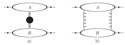
According to Eq. (58), the amplitude at LL comes solely from the factorized diagram shown in Fig. 6a, but without any gluon self-energy corrections. The jet $A$, containing lines moving in the plus direction, and jet $B$, consisting of lines moving in the minus direction, interact via the exchange of a single soft gluon. This gluon couples to jet $A$ via the $-$ component of its polarization and to jet $B$ via the $+$ component of its polarization. Since $v_{A}^{\alpha}\,N_{\alpha\,\beta}(q,\eta)\,v_{B}^{\beta}=1$, we can write at LL

$$A_{\bf 8}\,b_{\bf 8}=-\frac{1}{t}J_{A}^{(1)\,a}(p_{A},q,\eta)\,J_{B}^{(1)\,a}(p_{B},q,\eta),$$ (67)

where $b_{\bf 8}$ is the color basis vector corresponding to the octet exchange, defined in Eq. (2). Using $s=2p_{A}^{+}\,p_{B}^{-}$, the logarithmic derivative of the amplitude can be expressed as

$$\frac{\partial A_{\bf 8}}{\partial\ln s}\,b_{\bf 8}=-\frac{1}{t}\frac{\partial J_{A}^{(1)\,a}}{\partial\ln p_{A}^{+}}\,J_{B}^{(1)\,a}=-\frac{1}{t}\,J_{A}^{(1)\,a}\,\frac{\partial J_{B}^{(1)\,a}}{\partial\ln p_{B}^{-}}\;.$$ (68)

In Sec. 4.2, Eq. (33), we have derived an evolution equation resumming $\ln(p_{A}^{+})$ in $J_{A}^{(1)}$. We note that $J_{A}^{(1)}=\Gamma_{A}^{(1)}$, and that (33) is a special case of the evolution equation (51). The diagrammatic representation of the first term on the far right hand side of Eq. (33), which follows from Fig. 4 in the case when we have one external soft gluon attached to a jet function, is given by the diagrams in Fig. 7. Diagram in Fig. 7a corresponds to Fig. 4b and the diagrams in Figs. 7b and 7c correspond to Fig. 4a for $n=1$.

Figure 7: Diagrammatic representation of the evolution equation for jet $J_{A}^{(1)}$ at LL.

The diagrams in Figs. 7b and 7c are in the factorized form, while the one in Fig. 7a is not.

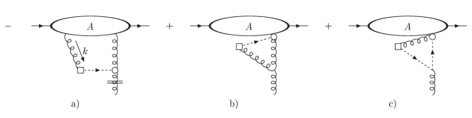
As discussed in Sec. 4.2, power counting shows that the loop momentum $k$ in Fig. 7a must be soft. This implies that we can make the following approximations. First, since at LL all internal lines of the jet $A$ are collinear to the $+$ direction, we can neglect the $k^{+}$ dependence of $J_{A}^{(2)}$, i.e. we may set $k^{+}=0$ inside $J_{A}^{(2)}$. Also, we can pick the plus components of the vertices where the soft gluons attach to the jet $J_{A}^{(2)}$. A short calculation, which uses the Feynman rules for special lines and vertices listed in Appendix D, gives the contribution to Fig. 7a in a form

$$\mathrm{Fig.}\;\ref{lleq}\mathrm{a} = -{\bar{g}}_{s}\,t\,f_{acb}\,\int\frac{{\mathrm{d}}^{D}k}{(2\pi)^{D}}\,\frac{1}{k^{2}(k-q)^{2}\,k\cdot{\bar{k}}}\,v_{A}^{\rho}N_{\rho\mu}(k)S^{\mu}(k)\;v_{B}^{\alpha}N_{\alpha\nu}(q-k)v_{A}^{\nu}$$ (69)

$$\times v_{B}^{\beta}\,v_{B}^{\gamma}\;J_{(A)\;\beta\,\gamma}^{(2)\,bc}\left(p_{A},q,\eta;k^{+}=0,k^{-},k_{\perp}\right),$$

Figure 8: Diagrams determining the contributions to the gluon trajectory at the order ${\alpha}_{s}$.

where we have defined ${\bar{g}}_{s}\equiv g_{s}{\mu}^{\epsilon}$. Using Eqs. (2) and (4.2) for the components of the gluon propagator and the boxed vertex, respectively, it is easy to see that in the Coulomb (Glauber) region, $k^{-}\ll k^{+}\sim k_{\perp}$, the integrand in Eq. (69) becomes an antisymmetric function of $k^{+}$ and that therefore the integration over $k^{+}$ vanishes in this region.

In the soft region, where all the components of soft momenta are of the same size $\sqrt{-t}$, we can use the $K$-$G$ decomposition for the soft gluon with momentum $k$ attached to $J_{A}^{(2)}$. At LL, however, there cannot be any soft internal lines in $J_{A}^{(2)}$ in Eq. (69), since, as discussed in Sec. 5.3, only integrals over collinear momenta can produce powers of $\ln p_{A}^{+}$. Therefore, at LL, only the $K$ gluon contributes, because the $G$ gluon must be attached to a soft line. The $K$ gluon can be decoupled from the rest of the jet $J^{(2)}_{A}$ using the Ward identities, Eq. (4.1). Their application in Eq. (69) gives

$$\mathrm{Fig.}\;\ref{lleq}\mathrm{a} = -i{\bar{g}}_{s}^{2}C_{A}t\,\int\frac{{\mathrm{d}}^{D}k}{(2\pi)^{D}}\,\frac{1}{k^{2}(k-q)^{2}\,k\cdot{\bar{k}}\,v_{A}\cdot k}\,v_{A}^{\rho}N_{\rho\mu}(k)S^{\mu}(k)\;v_{B}^{\alpha}N_{\alpha\nu}(q-k)v_{A}^{\nu}$$ (70)

$$\times J_{A}^{(1)\,a}(p_{A},q,\eta).$$

We have used the identity $f_{acb}\,f_{dcb}=N_{c}\,{\delta}_{ad}\equiv C_{A}\,{\delta}_{ad}$ in Eq. (70). Eq. (70) now gives a factorized form for Fig. 7a. Since the contributions in Figs. 7b and 7c are already in the factorized form, we can immediately infer that the gluon reggeizes at LL. Combining the terms from Fig. 7 in Eq. (33), we obtain the evolution equation at leading logarithm

$$p_{A}^{+}\frac{\partial}{\partial p_{A}^{+}}J_{A}^{(1)\,a}(p_{A},q,\eta)=\alpha(t)\,J_{A}^{(1)\,a}(p_{A},q,\eta).$$ (71)

Using the notation for evolution kernels introduced in Sec. 5.4, Eq. (71) implies that

$${\cal K}^{(1,2;1)}=0.$$ (72)

In Eq. (71)

$$\alpha(t)\equiv 1+{\alpha}^{(1)}_{a}(t)+{\alpha}^{(1)}_{b}(t)+{\alpha}^{(1)}_{c}(t),$$ (73)

is the gluon trajectory up to the order ${\alpha}_{s}$, and ${\alpha}^{(1)}_{a}(t)$, ${\alpha}^{(1)}_{b}(t)$ and ${\alpha}^{(1)}_{c}(t)$ are its contributions given in Figs. 8a - 8c, respectively,

$${\alpha}^{(1)}_{a}(t) \equiv -i{\bar{g}}_{s}^{2}C_{A}t\,\int\frac{{\mathrm{d}}^{D}k}{(2\pi)^{D}}\,\frac{1}{k^{2}(k-q)^{2}\,k\cdot{\bar{k}}\,v_{A}\cdot k}\,v_{A}^{\rho}N_{\rho\mu}(k)S^{\mu}(k)\;v_{B}^{\beta}N_{\beta\nu}(q-k)v_{A}^{\nu},$$

$${\alpha}^{(1)}_{b}(t) \equiv i{\bar{g}}_{s}^{2}C_{A}\,\int\frac{{\mathrm{d}}^{D}k}{(2\pi)^{D}}\,\frac{1}{k^{2}(k-q)^{2}\,k\cdot{\bar{k}}}\,S_{\alpha}(k)N^{\alpha\,\mu}(k)\;v_{A}^{\rho}N_{\rho}^{\;\;\nu}(q-k)\;V_{\mu\beta\nu}(k,-q,q-k)v_{B}^{\beta},$$

$${\alpha}^{(1)}_{c}(t) \equiv -i{\bar{g}}_{s}^{2}C_{A}\,\int\frac{{\mathrm{d}}^{D}k}{(2\pi)^{D}}\,\frac{1}{k^{2}\,k\cdot{\bar{k}}\,(q-k)\cdot({\bar{q}}-{\bar{k}})}\,v_{A}^{\rho}N_{\rho\mu}(k)S^{\mu}(k)\;(v_{B}\cdot{\bar{k}})\,.$$ (74)

In Eq. (6.1), $V_{\mu\beta\nu}(k,-q,q-k)$ stands for the momentum part of the three-point gluon vertex. After contracting the tensor structures in Eq. (6.1), using the explicit form for $V_{\mu\beta\nu}$, $v_{A}$, $v_{B}$, $S^{\mu}$ (Eq. (34)) and for the components of the gluon propagator, Eq. (2), we obtain for ${\alpha}^{(1)}_{a,b,c}(t)$,

$${\alpha}^{(1)}_{a}(t) = -i{\bar{g}}_{s}^{2}C_{A}\frac{t}{2}\,\int\frac{{\mathrm{d}}^{D}k}{(2\pi)^{D}}\frac{[k_{\perp}^{2}k_{0}+k^{2}k_{3}][(k-q)^{2}-(k-q)^{2}_{\perp}]}{(k_{0}+k_{3})\,k^{2}\,(k-q)^{2}\,(k\cdot{\bar{k}})^{2}\,(k-q)\cdot({\bar{k}}-{\bar{q}})}\;,$$

$${\alpha}^{(1)}_{b}(t) = i{\bar{g}}_{s}^{2}C_{A}\frac{1}{2}\,\int\frac{{\mathrm{d}}^{D}k}{(2\pi)^{D}}\frac{1}{k^{2}\,(k-q)^{2}\,(k\cdot{\bar{k}})^{2}\,(k-q)\cdot({\bar{k}}-{\bar{q}})}$$

$$\times [k_{\perp}^{2}\,{\bar{k}}^{2}\,(k-q)^{2}+2k^{2}\,k_{3}^{2}\,(k-q)_{\perp}\cdot q_{\perp}+2k_{0}^{2}\,k_{3}^{2}\,k_{\perp}\cdot(k-q)_{\perp}+2k_{0}^{2}\,k_{\perp}^{2}\,(k-q)_{\perp}^{2}]\;,$$

$${\alpha}^{(1)}_{c}(t) = i{\bar{g}}_{s}^{2}C_{A}\frac{1}{2}\,\int\frac{{\mathrm{d}}^{D}k}{(2\pi)^{D}}\frac{k_{3}^{2}}{(k\cdot{\bar{k}})^{2}\,(k-q)\cdot({\bar{k}}-{\bar{q}})}\;.$$ (75)

Next, we perform the $k^{0}$ and $k^{3}$ integrals in Eq. (6.1). For ${\alpha}^{(1)}_{a}(t)$, these integrals are UV/IR finite. However in the case of ${\alpha}^{(1)}_{b,c}(t)$, the $k^{0}$ integral is linearly UV divergent. In order to regularize this energy integral, we invoke split dimensional regularization introduced in Ref. [37]. The idea is to regularize separately the energy and the spatial momentum integrals, i.e. to write ${\mathrm{d}}^{4}k_{E}\rightarrow{\mathrm{d}}^{D_{1}}k_{4}\,{\mathrm{d}}^{D_{2}}{\vec{k}}$ for Euclidean loop momenta $k_{E}$. The dimensions $D_{1}$ and $D_{2}$ are given by $D_{1}=1-2{\varepsilon}_{1}$ and $D_{2}=3-2{\varepsilon}_{2}$, with ${\varepsilon}_{j}\rightarrow 0+$ for $j=1,2$. Since the energy integral for ${\alpha}^{(1)}_{c}(t)$ is scaleless, it vanishes in this split dimensional regularization. The energy integrals in ${\alpha}^{(1)}_{a,b}(t)$ are straightforward.

All the $k^{3}$ integrals can be expressed as derivatives with respect to $k_{\perp}^{2}$ and/or $(k-q)_{\perp}^{2}$ of a single integral

$$I(a,b)\equiv\int_{0}^{\infty}{\mathrm{d}}k^{3}\frac{1}{\sqrt{k^{2}_{3}+a^{2}}\;(k^{2}_{3}+b^{2})}=\frac{1}{b\sqrt{b^{2}-a^{2}}}\,\ln\left(\frac{b+\sqrt{b^{2}-a^{2}}}{a}\right).$$ (76)

The result of these integrations over $k^{3}$ is

$${\alpha}^{(1)}_{a}(t) = {\alpha}_{s}{\mu}^{2\epsilon}\,C_{A}\,t\,\int\frac{{\mathrm{d}}^{D-2}k_{\perp}}{(2\pi)^{D-2}}\left(I(|k_{\perp}|,|k_{\perp}-q_{\perp}|)\,\frac{k_{\perp}^{2}}{[(k-q)_{\perp}^{2}-k_{\perp}^{2}]^{2}}+\frac{2(k-q)_{\perp}^{2}-3k_{\perp}^{2}}{k_{\perp}^{2}\,[(k-q)_{\perp}^{2}-k_{\perp}^{2}]^{2}}\right),$$

$${\alpha}^{(1)}_{b}(t) = -{\alpha}_{s}{\mu}^{2\epsilon}\,C_{A}\,t\,\int\frac{{\mathrm{d}}^{D-2}k_{\perp}}{(2\pi)^{D-2}}\left(I(|k_{\perp}|,|k_{\perp}-q_{\perp}|)\,\frac{k_{\perp}^{2}}{[(k-q)_{\perp}^{2}-k_{\perp}^{2}]^{2}}-\frac{1}{[(k-q)_{\perp}^{2}-k_{\perp}^{2}]^{2}}\right),$$

$${\alpha}^{(1)}_{c}(t) = 0.$$ (77)

Combining the results of Eq. (6.1) and Eq. (73), we obtain the standard expression for the gluon trajectory at LL

$$\alpha(t)=1+C_{A}{\alpha}_{s}{\mu}^{2\epsilon}\,\int\frac{{\mathrm{d}}^{D-2}k_{\perp}}{(2\pi)^{D-2}}\frac{t}{k_{\perp}^{2}\,(k-q)_{\perp}^{2}}\;.$$ (78)

We can now simply solve the evolution equation (68), to derive the factorized (reggeized) form for the amplitude in the color octet

$$A_{\bf 8}(s,t,{\alpha}_{s})=s^{\alpha(t)}\,{\tilde{A}}_{\bf 8}(t,{\alpha}_{s}).$$ (79)

The amplitude factorizes into the universal factor $s^{\alpha(t)}$, which is common for all processes involving two partons in the initial and final state and dominated by the gluon exchange, and the part ${\tilde{A}}_{\bf 8}$, the so-called impact factor, which is specific to the process under consideration.

6.2 Amplitude at NLL

At NLL level the contribution to the amplitude comes from both the one gluon exchange diagram, Fig. 6a, and from the two gluon exchange diagram, Fig. 6b. At this level, both singlet and octet color exchange are possible in the latter. Including the self-energy corrections to the propagator of the exchanged gluon (taking into account the corresponding counter-terms), we can write the contribution from the diagram in Fig. 6a as follows,

$$A^{(1)}\equiv-\frac{1}{t}\,J_{(A)\,\alpha}^{(1)\,a}\,(p_{A},q,\eta)\,\left(N^{\alpha\beta}(q,\eta)+\frac{1}{t}\,v_{B}^{\alpha}\,v_{A}^{\mu}\,{\Pi}_{\mu\,\nu}(q,\eta)\,v_{B}^{\nu}\,v_{A}^{\beta}\right)\,J_{(B)\,\beta}^{(1)\,a}\,(p_{B},q,\eta),$$ (80)

where ${\Pi}_{\mu\,\nu}(q,\eta)$ stands for the one loop gluon self-energy. We now put this contribution into the first factorized form, Eq. (27), isolating the plus polarization for jet A, and the minus polarization for jet B. At NLL in the amplitude, we need the soft function $S^{(1,1)}$, Eq. (27) with $n=m=1$, to accuracy ${\cal O}(\alpha_{s})$. Using the tulip-garden formalism described in Appendix C, the contribution to the first term on the right hand side of Eq. (80) is given by the subtractions shown in Fig. 9. In accordance with the notation adopted in Appendix C, the dashed lines indicate that we have made soft approximations on gluons that are cut by them. A dashed line cutting a gluon attached to jet $A$($B$) means that the gluon is attached to the corresponding jet through minus(plus) component of its polarization. Since $q^{\pm}=0$ in the Regge limit, Eq. (2), we have $N^{\mu\pm}(q)=g^{\mu\pm}$. This implies that the contributions between the diagrams in Fig. 9c and in Fig. 9d as well as between the diagrams in Fig. 9e and in Fig. 9f cancel each other. Therefore only the zeroth-order soft function diagram in Fig. 9b survives in the factorized form, Eq. (27).

Figure 9: Expansion of the one gluon exchange amplitude at NLL using the tulip garden formalism.

For the two gluon exchange, Fig. 6b, we only need the lowest order soft function at NLL in the amplitude (and LL in singlet exchange). The expression for the two gluon exchange diagram in Fig. 6b takes the form, Eq. (27),

$$A^{(2)}=\int\frac{{\rm d}^{D}k}{(2\pi)^{D}}\,J_{A}^{(2)\;a\,b}(k^{+}=0,k^{-},k_{\perp})\,S(k^{+},k^{-},k_{\perp})\,J_{B}^{(2)\;a\,b}(k^{-}=0,k^{+},k_{\perp}),$$ (81)

where $S(k)$ is given by

$$S(k)\equiv\frac{i}{2!}\,\frac{N^{-\,+}(k)}{k^{2}+i\epsilon}\,\frac{N^{-\,+}(q-k)}{(q-k)^{2}+i\epsilon}.$$ (82)

We have suppressed the dependence of the functions appearing in Eq. (81) on other arguments for brevity. At NLL accuracy we are entitled to pick the plus Lorentz indices for jet function $J_{A}$ and the minus indices for jet function $J_{B}$ only. We can also set $k^{+}=0$ in $J_{A}$ and $k^{-}=0$ in $J_{B}$ since all the loop momenta inside the jets are collinear. Eq. (81) represents the first factorized form, Eq. (27), for the amplitude $A^{(2)}$.

Next, we follow the procedure described in Sec. 5.1 to bring the amplitude into the second factorized form, Eq. (40). We employ an identity based on Eq. (44), for the function $S(k)$ defined in Eq. (82)

$$S(k^{+},k^{-}) = S(k^{+}=0,k^{-}=0)\,\theta(M-|k^{+}|)\,\theta(M-|k^{-}|)$$

$$+ [S(k^{+},k^{-}=0)-S(k^{+}=0,k^{-}=0)\,\theta(M-|k^{+}|)]\,\theta(M-|k^{-}|)$$

$$+ [S(k^{+}=0,k^{-})-S(k^{+}=0,k^{-}=0)\,\theta(M-|k^{-}|)]\,\theta(M-|k^{+}|)$$

$$+ [\{S(k^{+},k^{-})-S(k^{+},k^{-}=0)\,\theta(M-|k^{-}|)\}-$$

$$\{S(k^{+}=0,k^{-})-S(k^{+}=0,k^{-}=0)\,\theta(M-|k^{-}|)\}\,\theta(M-|k^{+}|)].$$

The contribution from the first term in Eq. (6.2) gives immediately the second factorized form with $\Gamma^{(2)}_{A}$ and $\Gamma^{(2)}_{B}$ defined in Eq. (5.1) for $n=m=2$.

We now discuss the rest of the terms in Eq. (6.2), which can be analyzed using the $K$-$G$ decomposition, since, by construction, there is no contribution from the Glauber region. At the current accuracy only the $K$-gluon contributes. After substituting the second term of Eq. (6.2) into Eq. (81), we can factor the gluon with momentum $k$ from jet $J_{B}^{(2)}$. However, it is easy to verify, using the definitions for $K$ and $G$ gluons, Eq. (4.1), the Ward identities, Eq. (4.1), and the explicit components of the gluon propagator, Eq. (2), that the $k^{+}$ integral is over an antisymmetric function. As a result, this contribution vanishes. In a similar fashion, the contribution from the third term in Eq. (6.2), after used in Eq. (81), vanishes, since now we can factor the soft gluon with momentum $k$ from jet $J_{A}^{(2)}$ and the $k^{-}$ integral is over an antisymmetric function.

In the case of the last term in Eq. (6.2), after used in Eq. (81), we can factor the soft gluon with momentum $k$ from both jets $J_{A}^{(2)}$ and $J_{B}^{(2)}$. The integrals of the soft function $S(k)$ over $k^{+}$ and $k^{-}$ are then

$$\tilde{S}(k_{\perp},q;M)\equiv C_{A}\,\frac{g_{s}^{2}}{(2\pi)^{2}}\,\int_{-M}^{M}\frac{{\rm d}k^{+}}{k^{+}}\,\frac{{\rm d}k^{-}}{k^{-}}\,S(k^{+},k^{-},k_{\perp},q).$$ (84)

As usually, we leave the transverse momentum integral undone. The $1/k^{+}$ and $1/k^{-}$ in the integral above are given by the Principal Value prescription because there is no contribution from the Glauber region. Since the amplitude is independent on the choice of scale $M$, we can evaluate it at arbitrary scale. We choose to work in the limit $M\rightarrow 0$. In this limit the contribution to the integral comes from the imaginary parts of the gluon propagators in Eq. (82), $-i\pi\delta(k^{2})$ and $-i\pi\delta((k-q)^{2})$. The integration is then trivial and Eq. (84) becomes

$$\tilde{S}(k_{\perp},q)\equiv\lim_{M\rightarrow 0}\tilde{S}(k_{\perp},q;M)\equiv-C_{A}\,\frac{ig_{s}^{2}}{8}\,\frac{1}{k_{\perp}^{2}\,(k-q)^{2}_{\perp}}.$$ (85)

Combining the partial results of the analysis described above in Eq. (81), we arrive at the second factorized form for the double gluon exchange amplitude, Fig. 6b,

$$A^{(2)} = \int\frac{{\rm d}^{D-2}k_{\perp}}{(2\pi)^{D-2}}\,{\Gamma}_{A}^{(2)\;a\,b}(k_{\perp})\,\frac{1}{(2\pi)^{2}}\,S(k^{+}=0,k^{-}=0,k_{\perp})\,{\Gamma}_{B}^{(2)\;a\,b}(k_{\perp})$$ (86)

$$+ \int\frac{{\rm d}^{D-2}k_{\perp}}{(2\pi)^{D-2}}\,{\Gamma}_{A}^{(1)\;a}(p_{A},q)\;\tilde{S}(k_{\perp},q)\;{\Gamma}_{B}^{(1)\;a}(p_{A},q).$$

Using Eq. (80) for $A^{(1)}$ and Eq. (86) for $A^{(2)}$, we obtain the amplitude for the process (1) at NLL accuracy

$$A^{({\rm NLL})} = -\frac{1}{t}\,\Gamma_{A}^{(1)\,a}\,(p_{A},q,\eta)\,\left(1+\frac{1}{t}\,{\Pi}_{+\,-}(q,\eta)+\frac{i\pi}{2}\,\alpha^{(1)}(t)\right)\,\Gamma_{B}^{(1)\,a}\,(p_{B},q,\eta)$$ (87)

$$+ \int\frac{{\rm d}^{D-2}k_{\perp}}{(2\pi)^{D-2}}\,{\Gamma}_{A}^{(2)\;a\,b}(k_{\perp})\,\frac{i}{8\pi^{2}}\,\frac{1}{k_{\perp}^{2}\,(k-q)^{2}_{\perp}}\,{\Gamma}_{B}^{(2)\;a\,b}(k_{\perp}).$$

In Eq. (87), we have used the explicit form for $S(k^{+}=0,k^{-}=0,k_{\perp})$, which can be easily identified from Eq. (82). We have also used the integral representation of the gluon trajectory given in Eq. (78).

In order to determine the high energy behavior of the amplitude in Eq. (87), we need to examine the high energy behavior of $\Gamma_{A}^{(1)}$ or $\Gamma_{B}^{(1)}$ at NLL and the evolution of $\Gamma_{A}^{(2)}$ or $\Gamma_{B}^{(2)}$ at LL. In this paper, we restrict the discussion of evolution equations to LL level, and hence we analyze the behavior of $\Gamma_{A}^{(2)}$ only. We will address the study of NLL jet evolution, and gluon reggeization at this level, elsewhere [39].

We use the evolution equation given by Eq. (51) in order to determine the LL dependence of $\Gamma_{A}^{(2)}$ on $\ln(p_{A}^{+})$. In our special case of the two gluon exchange amplitude, it reads

$$\left(p_{A}^{+}\,\frac{\partial}{\partial\,p_{A}^{+}}-1\right){\Gamma}_{A}^{(2)\;a\,b} = M\,\left[J_{A}^{(2)\;a\,b}(k^{-}=+M,k^{+}=0,k_{\perp})+J_{A}^{(2)\;a\,b}(k^{-}=-M,k^{+}=0,k_{\perp})\right]$$ (88)

$$- {\tilde{\eta}}^{\alpha}\frac{\partial}{\partial\,{\eta}^{\alpha}}\,\Gamma_{A}^{(2)\;a\,b}.$$

Figure 10: Diagrams determining the evolution of $\Gamma_{A}^{(2)}$.

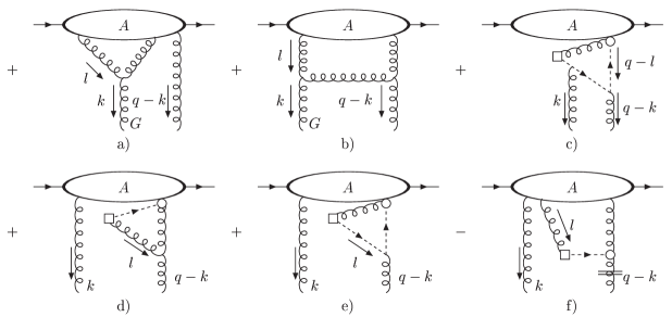
The first term in Eq. (88) can be analyzed using the $K$-$G$ decomposition. The contributions from the $K$-gluon cancel between the $J_{A}^{(2)}(k^{-}=+M)$ and $J_{A}^{(2)}(k^{-}=-M)$. The contributions from the $G$ gluon, which we now discuss, are shown in Figs. 10a and 10b.

Since the gluon with momentum $q-k$ in Fig. 10a cannot be in the Glauber region, we can use $K$-$G$ decomposition on it. The $K$ part factors from $J_{A}^{(3)}$, while the $G$ part does not contribute at LL. After factoring out the gluon with momentum $q-k$ and performing the approximations on the jet function $J_{A}^{(2)}$, the contribution to Fig. 10a for $k^{-}=+M$ is

$${\rm Fig.\;\ref{bfklDiagrams}a}=-ig_{s}^{2}f_{aec}f_{deb}\,\frac{1}{M}\int\frac{{\rm d}^{D}l}{(2\pi)^{D}}\,S_{1}(k^{+}=0,k^{-}=+M,k_{\perp},l)\;J_{A}^{(2)\,c\,d}(l^{+}=0,l^{-},l_{\perp}),$$ (89)

where we have defined

$$S_{1}(k,l)\equiv\frac{N^{-\,\mu}(l)}{l^{2}}\,\frac{N^{-\,\nu}(k-l)}{(k-l)^{2}}\,V_{\mu\,\rho\,\nu}(l,-k,k-l)\,\left(g^{\rho\,+}-\frac{k^{\rho}}{M}\right).$$ (90)

Next we follow the established procedure. First, we write

$$S_{1}(k,l)=S_{1}(k,l^{-}=0)\,\theta(M-|l^{-}|)+\left[S_{1}(k,l)-S_{1}(k,l^{-}=0)\,\theta(M-|l^{-}|)\right].$$ (91)

When we use the second term of Eq. (91) in Eq. (89), we can factor the gluon with momentum $l$ from $J_{A}^{(2)}$. Since the resulting integrand is an antisymmetric function under the simultaneous transformation $M\rightarrow-M$, $l^{\pm}\rightarrow-l^{\pm}$, the contributions on the right hand side of Eq. (88) evaluated for $k^{-}=+M$ and $k^{-}=-M$ cancel each other. Therefore we can write, using Eq. (91) in Eq. (89),

$${\rm Fig.\;\ref{bfklDiagrams}a} = -ig_{s}^{2}\,f_{aec}f_{deb}\,\frac{1}{M}\int\frac{{\rm d}^{D-2}l_{\perp}}{(2\pi)^{D}}\,\int{\rm d}l^{+}\,S_{1}(k^{+}=0,k^{-}=+M,k_{\perp},l^{-}=0,l^{+},l_{\perp})\;{\Gamma}_{A}^{(2)\,c\,d}(l_{\perp})$$ (92)

$$+ \ldots,$$

where by dots we mean the term which is canceled after we take into account the contributions to both $J_{A}^{(2)}(k^{-}=+M)$ and $J_{A}^{(2)}(k^{-}=-M)$ on the right hand side of Eq. (88).

Next, we perform the $l^{+}$ integral in Eq. (92). As we have already mentioned above, since the final result does not depend on the scale $M$, we can choose arbitrary value of $M$. We have chosen to perform the calculation in the limit $M\rightarrow 0$. Then the only nonvanishing contribution comes from the imaginary part of the propagator $1/[(l-k)^{2}+i\epsilon]$, $-i\pi\,\delta(2Ml^{+}+(l-k)^{2}_{\perp})$. For this term the $l^{+}$ integration is trivial and we obtain

$$M\,({\rm Fig.\;\ref{bfklDiagrams}a})=-\alpha_{s}\,f_{aec}f_{deb}\,\int\frac{{\rm d}^{D-2}l_{\perp}}{(2\pi)^{D-2}}\,\frac{2k_{\perp}\cdot l_{\perp}}{l_{\perp}^{2}\,(k-l)_{\perp}^{2}}\;{\Gamma}_{A}^{(2)\,c\,d}(l_{\perp})+\ldots\,,$$ (93)

which gives an $M$-independent contribution to the right hand side of Eq. (89).

We follow the same steps when dealing with the diagram in Fig. 10b, whose soft subdiagram is given by

$$S_{2}(k,l)\equiv\frac{N^{-\,\mu}(l)}{l^{2}}\,\frac{N^{-\,\nu}(q-l)}{(q-l)^{2}}\,V_{\mu\,\rho\,\gamma}(l,-k,k-l)\,\left(g^{\rho\,+}-\frac{k^{\rho}}{M}\right)\frac{N^{\gamma\delta}(l-k)}{(l-k)^{2}}\,V_{\nu\,\delta\,-}(q-l,l-k,k-q).$$ (94)

First we use the identity (91) for $S_{2}$. The contribution due to the second term in Eq. (91) vanishes, after the gluon with momentum $l$ has been factored from $J_{A}^{(2)}$, due to the antisymmetry of the integrand. Hence again, as in the case discussed above, only the term given by $S_{2}(l^{-}=0,l^{+},l_{\perp},k)$ contributes. In the limit $M\rightarrow 0$, the contribution comes from the imaginary part of the same denominator as in the case of Fig. 10a. The result is

$$M\,({\rm Fig.\;\ref{bfklDiagrams}b})= - \alpha_{s}\,f_{aec}f_{deb}\,\int\frac{{\rm d}^{D-2}l_{\perp}}{(2\pi)^{D-2}}\,\frac{2}{l_{\perp}^{2}\,(l-q)^{2}_{\perp}\,(k-l)_{\perp}^{2}}$$ (95)

$$\times \left(k_{\perp}^{2}l_{\perp}^{2}-k_{\perp}\cdot l_{\perp}l_{\perp}^{2}-k_{\perp}\cdot q_{\perp}l_{\perp}^{2}-k_{\perp}^{2}l_{\perp}\cdot q_{\perp}+2k_{\perp}\cdot l_{\perp}l_{\perp}\cdot q_{\perp}\right)\times{\Gamma}_{A}^{(2)\,c\,d}(l_{\perp})$$

$$+ \ldots\,.$$

Combining the results of Eqs. (93) and (95), we obtain the expression for the surface term in Eq. (88)

$$M\left[J_{A}^{(2)\;a\,b}(k^{-}=+M,k^{+}=0,k_{\perp})+J_{A}^{(2)\;a\,b}(k^{-}=-M,k^{+}=0,k_{\perp})\right]=2\alpha_{s}\,f_{aec}f_{bed}$$

$$\times \int\frac{{\rm d}^{D-2}l_{\perp}}{(2\pi)^{D-2}}\left(\frac{k_{\perp}^{2}}{l_{\perp}^{2}\,(k-l)_{\perp}^{2}}+\frac{(k-q)_{\perp}^{2}}{(l-q)_{\perp}^{2}\,(k-l)_{\perp}^{2}}-\frac{q_{\perp}^{2}}{l_{\perp}^{2}\,(q-l)_{\perp}^{2}}\right)\,\times{\Gamma}_{A}^{(2)\,c\,d}(l_{\perp}).$$ (96)

Next, we analyze the contributions to the term ${\tilde{\eta}}^{\alpha}\partial/\partial\,{\eta}^{\alpha}\,\Gamma_{A}^{(2)}$ in the evolution equation (88). The contributing diagrams are shown in Figs. 10c - 10f. Note that for every diagram in Figs. 10c - 10f, we have also diagrams when a loop containing the boxed vertex is attached to the external gluon with momentum $k$, instead of to the external gluon with momentum $q-k$.

In Fig. 10c, we have to consider all the possible insertions of external gluons with momenta $k$ and $q-k$. We have six possibilities. The contribution shown in Fig. 10c is proportional to (omitting the color factor)

$$\int_{-M}^{M}{\rm d}k^{-}\,({\rm Fig.\;\ref{bfklDiagrams}c})\propto\int_{-M}^{M}{\rm d}k^{-}\,\int\frac{{\rm d}^{D}l}{(2\pi)^{D}}\frac{N^{-\,\mu}(l)}{l^{2}}\frac{S_{\mu}(l)}{l\cdot{\bar{l}}}\,\frac{(\bar{l}-\bar{k})^{+}}{(\bar{l}-\bar{k})^{2}}\,\frac{(\bar{q}-\bar{l})^{+}}{(\bar{q}-\bar{l})^{2}}\,(k^{+}=0).$$ (97)

Since the integrand is an antisymmetric function under $k^{-}\rightarrow-k^{-}$ and $l^{\pm}\rightarrow-l^{\pm}$, the integral in Eq. (97) vanishes. The same antisymmetry property holds for the remaining five diagrams and therefore, there is no contribution from them.

Figure 11: Contributions to the diagram in Fig. 10f when the gluon coming out of the boxed vertex is attached to the soft line (a) and when either or both gluons with momenta $k$ and $l$ are $K$ gluons and they are factored from the jet (b - f).

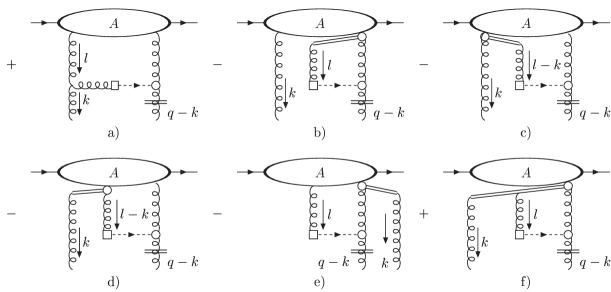
Let us next focus on the diagram in Fig. 10f. When the gluon with momentum $l$ attaches to a soft line inside of the jet $J_{A}^{(3)}$, the contribution takes the form shown in Fig. 11a. If it attaches to a jet line, its contribution can be written as

$${\rm Fig.\;\ref{bfklDiagrams}f}=-g_{s}f_{bcd}\,\int\frac{{\rm d}^{D}l}{(2\pi)^{D}}\,S_{3}(k^{+}=0,k^{-},k_{\perp},l)\;J_{A}^{(3)\,a\,c\,d}(k^{+}=0,k^{-},k_{\perp},l^{+}=0,l^{-},l_{\perp}),$$ (98)

with the soft function

$$S_{3}(k,l)\equiv(q-k)^{2}\,\frac{N^{-\mu}(l)}{l^{2}}\,\frac{S_{\mu}(l)}{l\cdot\bar{l}}\,\frac{N^{-+}(q-k-l)}{(q-k-l)^{2}}.$$ (99)

We use the identity for this soft function $S_{3}$, obtained from Eq. (6.2) by the replacement $k^{+}\rightarrow l^{-}$,

$$S_{3}(l^{-},k^{-}) = S_{3}(l^{-}=0,k^{-}=0)\,\theta(M-|l^{-}|)\,\theta(M-|k^{-}|)$$ (100)

$$+ [S_{3}(l^{-},k^{-}=0)-S_{3}(l^{-}=0,k^{-}=0)\,\theta(M-|l^{-}|)]\,\theta(M-|k^{-}|)$$

$$+ [S_{3}(l^{-}=0,k^{-})-S_{3}(l^{-}=0,k^{-}=0)\,\theta(M-|k^{-}|)]\,\theta(M-|l^{-}|)$$

$$+ [\{S_{3}(l^{-},k^{-})-S_{3}(l^{-},k^{-}=0)\,\theta(M-|k^{-}|)\}$$

$$-\{S_{3}(l^{-}=0,k^{-})-S_{3}(l^{-}=0,k^{-}=0)\,\theta(M-|k^{-}|)\}\,\theta(M-|l^{-}|)],$$

to treat the soft gluons with momenta $k$ and $l$ attached to jet $J_{A}^{(3)}$. The contribution from the first term in Eq. (100), when used in Eq. (98), vanishes since the integrand $S_{3}(k^{+}=k^{-}=0,k_{\perp},l^{-}=0,l^{+},l_{\perp})$ is an antisymmetric function of $l^{+}$, as can be easily checked using Eqs. (2), (4.2) and (99). We can apply the $K$-$G$ decomposition on the gluon with momentum $l$ when treating the second term in Eq. (100) used in Eq. (98). At LL only the $K$ gluon contributes. It can be factored from the jet function $J^{(3)}_{A}$ with the result shown in Figs. 11b and 11c. In a similar way we can treat the gluon with momentum $k$ in the third term of Eq. (100). After we factor this gluon from the jet $J_{A}^{(3)}$, we obtain the contributions shown in Figs. 11d and 11e. In the case of the last term in Eq. (100), we can factor out both soft gluons with momenta $k$ and $l$ from jet $J_{A}^{(3)}$. The result of this factorization is shown in Fig. 11f.

Next, we note that the combination of the diagrams in Figs. 10d, 10e and 11b is the same as the result encountered in the analysis of the LL amplitude, Fig. 8. We write

$$\int_{-M}^{M}{\rm d}k^{-}\left({\rm Fig.\;\ref{bfklDiagrams}d}+{\rm Fig.\;\ref{bfklDiagrams}e}+{\rm Fig.\;\ref{bfklFact}b}\right)=\alpha^{(1)}(q_{\perp}-k_{\perp})\,\Gamma_{A}^{(2)\;a\,b}(p_{A},q,k_{\perp}).$$ (101)

where $\alpha^{(1)}(q-k)$ in Eq. (101) is given by the diagrams in Fig. 8 with an external momentum $q-k=(0^{+},0^{-},q_{\perp}-k_{\perp})$. In the case when the gluon coming out of the boxed vertex attaches to an external gluon with momentum $k$, we evaluate the one loop trajectory $\alpha^{(1)}(k_{\perp})$ in Eq. (101).

To complete the analysis, we have to discuss the diagrams in Figs. 11a and 11c - 11f. In the region $l^{\pm}\sim l_{\perp}$, we can factor the gluon with momentum $l$ from the jet function $J_{A}^{(2)}(l^{+}=0,l^{-},l_{\perp})$ in the case of the diagram in Fig. 11a. The resulting $k^{-}$ and $l^{\pm}$ integral is over an antisymmetric function of $k^{-}$ and $l^{\pm}$, and therefore it vanishes. So the only contribution comes from the Glauber region, where we can set $l^{-}=0$ outside $J_{A}^{(2)}(l^{+}=0,l^{-},l_{\perp})$. As above, we perform the $l^{+}$ and $k^{-}$ integrals in the limit $M\rightarrow 0$. The integrand does not develop a singularity in $k^{-}$ and/or $l^{+}$ strong enough to compensate for the shrinkage of the integration region $\int_{-M}^{M}{\rm d}k^{-}$ when $M\rightarrow 0$. Hence the diagram in Fig. 11a does not contribute in the limit $M\rightarrow 0$. In a similar way as for the diagram in Fig. 11a, none of the diagrams in Figs. 11c - 11f contribute. The diagrams in Figs. 11c - 11e vanish in the $M\rightarrow 0$ limit, while in the case of the diagram in Fig. 11f the $k^{-}$ and $l^{\pm}$ integral is over an antisymmetric function of $k^{-}$ and $l^{\pm}$.

At this point we have discussed all the contributions appearing on the right hand side of the evolution equation (88). Combining the partial results given by Eqs. (101) and (6.2) in Eq. (88), we arrive at the evolution equation governing the high energy behavior of $\Gamma_{A}^{(2)}$

$$\left(p_{A}^{+}\,\frac{\partial}{\partial\,p_{A}^{+}}-1\right){\Gamma}_{A}^{(2)\;a\,b}(p_{A}^{+},q,k_{\perp}) = 2\alpha_{s}\,f_{aec}f_{bed}\,\int\frac{{\rm d}^{D-2}l_{\perp}}{(2\pi)^{D-2}}\;\Gamma_{A}^{(2)\;c\,d}(p_{A}^{+},q,l_{\perp})$$ (102)

$$\times \left(\frac{k_{\perp}^{2}}{l_{\perp}^{2}\,(k-l)_{\perp}^{2}}+\frac{(k-q)_{\perp}^{2}}{(l-q)_{\perp}^{2}\,(k-l)_{\perp}^{2}}-\frac{q_{\perp}^{2}}{l_{\perp}^{2}\,(q-l)_{\perp}^{2}}\right)$$

$$+ \left(\alpha^{(1)}(k_{\perp})+\alpha^{(1)}(q_{\perp}-k_{\perp})\right)\times\Gamma_{A}^{(2)\;a\,b}(p_{A}^{+},q,k_{\perp}).$$

Projecting out onto the color singlet in Eq. (102), we immediately recover the celebrated BFKL equation [9].

6.3 Evolution of $\Gamma^{(n)}$ at LL

We can now generalize Eq. (102) to the case of $\Gamma_{A}^{(n)}$. The evolution kernel in this case contains, besides a piece diagonal in the number of external gluons, also contributions which relate jet functions with different number of external gluons

$$\left(p_{A}^{+}\,\frac{\partial}{\partial\,p_{A}^{+}}-1\right){\Gamma}_{A}^{(n)\;a_{1}\ldots\,a_{n}}(p_{A}^{+},q,k_{1\,\perp},\dots,k_{n\,\perp})=$$ (103)

$$2\alpha_{s}\,\sum_{i<j}^{n}f_{a_{i}\,e\,b_{i}}f_{a_{j}\,e\,b_{j}}\,\int\frac{{\rm d}^{D-2}l_{i\,\perp}}{(2\pi)^{D-2}}\,\frac{{\rm d}^{D-2}l_{j\,\perp}}{(2\pi)^{D-2}}\,\delta^{(2)}(l_{i\,\perp}+l_{j\,\perp}-k_{i\,\perp}-k_{j\,\perp})$$

$$\times\;\left(\frac{k_{i\,\perp}^{2}}{l_{i\,\perp}^{2}\,(k_{i}-l_{i})_{\perp}^{2}}+\frac{k_{j\,\perp}^{2}}{l_{j\,\perp}^{2}\,(k_{j}-l_{j})_{\perp}^{2}}-\frac{(k_{i}+k_{j})_{\perp}^{2}}{l_{i\,\perp}^{2}\,l_{j\,\perp}^{2}}\right)$$

$$\times\;\Gamma_{A}^{(n)\;a_{1}\ldots\,b_{i}\ldots\,b_{j}\ldots\,a_{n}}(p_{A}^{+},q,k_{1\,\perp},\ldots,l_{i\,\perp},\ldots,l_{j\,\perp},\ldots,k_{n\,\perp})$$

$$+\;\sum_{i=1}^{n}\left(\alpha^{(1)}(k_{i\,\perp})\right)\times{\Gamma}_{A}^{(n)\;a_{1}\ldots\,a_{n}}(p_{A}^{+},q,k_{1\,\perp},\dots,k_{n\,\perp})$$

$$+\;\sum_{n^{\prime}=1}^{n-1}{\cal K}^{(n,n^{\prime})}_{a_{1}\ldots\,a_{n};\;b_{1}\ldots\,b_{n^{\prime}}}\,{\otimes}_{\perp}\,{\Gamma}_{A}^{(n^{\prime})\;b_{1}\ldots\,b_{n^{\prime}}},$$

where ${\otimes}_{\perp}$ denotes a convolution in transverse momentum space. The last term in Eq. (103) corresponds to the configurations when one or more external gluons attach to a gluon or a ghost lines forming the one loop kernel derived for $\Gamma_{A}^{(2)}$. Using the notation of Sec. 5.4, we can write Eq. (103) at $r$-loop order in a form

$$\left(p_{A}^{+}\frac{\partial}{\partial p_{A}^{+}}-1\right)\Gamma_{A}^{(n,r)}=\sum_{n^{\prime}=1}^{n}{\cal K}^{(n,n^{\prime};1)}\otimes\Gamma_{A}^{(n^{\prime},r-1)}.$$ (104)

It corresponds to Eq. (64) of Sec. 5.4 when written in terms of the coefficients $c_{r}^{(n,r)}$ introduced in Eq. (60). From Eq. (104) we immediately see that the following property of the one loop kernel

$${\cal K}^{(n,n^{\prime};1)}=\theta(n-n^{\prime})\,{\tilde{\cal K}}^{(n,n^{\prime};1)},$$ (105)

is satisfied. We recall that this step was essential in demonstrating that the set of evolution equations, Eq. (51), forms a consistent system, refer to the paragraph above Eq. (64).

The term diagonal in the number of external gluons in Eq. (103) coincides with the evolution equation derived in Ref. [5]. Our formalism, besides enabling us to go systematically beyond LL accuracy, Ref. [39], indicates that even at LL, in addition to the kernels found in Ref. [5], the kernel has contributions which relate jet functions with different number of external gluons.

7 Conclusions

We have established a systematic method that shows that it is possible to resum the large logarithms appearing in the perturbation series of scattering amplitudes for $2\rightarrow 2$ partonic processes to arbitrary logarithmic accuracy in the Regge limit. Up to corrections suppressed by powers of $|t|/s$, the amplitude can be expressed as a sum of convolutions in transverse momentum space over soft and jet functions, Eq. (40). All the large logarithms are organized in the jet functions, Eq. (5.1). They are resummed using Eqs. (51) and/or (56). The evolution kernel $\cal K$ in Eq. (56) is a calculable function of its arguments order by order in perturbation theory. This is the central result of our analysis.

As an illustration of the general algorithm we have demonstrated it in an action at NLL for the amplitude and LL for the evolution equations. We reserve the study of the NLL evolution, which addresses the reggeization of a gluon at NLL, for future work [39].

The derivation of the evolution equations and the procedure for finding the kernels was given above in Coulomb gauge. Clearly, it will be useful and interesting to reformulate our arguments in covariant gauges. In addition, the connection of our formalism to the effective action approach to small-$x$ and the Regge limit, Refs. [23, 24] should provide further insight.

Acknowledgment

I wish to thank G. Sterman for suggesting this problem to me, for invaluable help and constant encouragement. I also wish to thank A. Sen for very helpful discussions. During the process of this work I have benefited from conversations with C.F. Berger, G.T. Bodwin, J.C. Collins, P.A. Grassi, M.E. Tejeda-Yeomans, A.R. White and K. Zoubos.

Appendix A Power counting with contracted vertices

In this appendix we will include the possibility of contracted vertices in the reduced diagram in Fig. 1a. These are associated with internal lines (collapsed to a point) which are off-shell by $\sqrt{s}$. Our analysis closely follows [27] and [31].

If we go back to the argument that led us to Eq. (15) for the superficial degree of IR divergence for the soft part, we see that the same reasoning as in the case of elementary vertices applies to the case of contracted vertices since the result (15) has been obtained by means of dimensional counting.

The analysis of contracted vertices connecting jet lines only is, however, more subtle. We have to demonstrate that the suppression factors corresponding to the contracted vertices are at least as great as the ones for the elementary vertices. The expression (22) tells us that we can restrict ourselves to the two and three point vertices. For these cases, we analyze the full two and three-point subdiagrams, by studying the tensor structures that are found after integration over their internal loop momenta.

Before we discuss all the possible structures, we state some results which will be essential for the upcoming analysis. The first one is the simple Dirac matrix identity

$$\not{\!a}\,\not{\!b}\,\not{\!a}=2(a\cdot b)\,\not{\!a}-a^{2}\,\not{\!b}.$$ (106)

The other two follow from Eqs. (7) and (2) for the gluon propagator in Coulomb gauge, and hold for any jet momenta scaling as $l_{A}\,\sim\,l_{A}^{\prime}\,\sim\,\sqrt{s}(1^{+},\lambda^{-},{\lambda}^{1/2})$ collinear to the momentum $p_{A}$ defined in Eq. (2)

$$l_{A}^{\prime\;\alpha}\,N_{\alpha\beta}(l_{A},\eta) = {\cal O}({\lambda}^{1/2}\,\sqrt{s}),$$

$${\bar{l}}_{A}^{\prime\;\alpha}\,N_{\alpha\beta}(l_{A},\eta) = {\cal O}({\lambda}^{1/2}\,\sqrt{s}),$$ (107)

for all components of $\beta$. We now proceed to discuss the particular cases.

Ghost self-energy: The most general covariant structure is, using $p\cdot\bar{p}={\bar{p}}^{2}$,

$$\Pi(p,\bar{p})=p\cdot{\bar{p}}\,f(p^{2}/{\mu}^{2},\,{\bar{p}}^{2}/{\mu}^{2},\,{\alpha}_{s}(\mu)),$$ (108)

where $\mu$ is a scale introduced by a UV/IR regularization of Feynman diagrams and $p$ is the momentum of an internal jet line. Strictly speaking, the covariants should be formed from the vectors $p$ and $\eta$, but since $p$ has nonzero light-cone components, we can use Eq. (8), to express $\eta$ in terms of $\bar{p}$. The maximum degree of divergence for the ghost self-energy occurs when the internal lines become either parallel to the external momentum $p$ or soft. The most general pinch singular surface consists of a subdiagram of collinear lines moving in a direction of the external ghost. This subdiagram can interact with itself through the exchange of soft quanta. Power counting arguments similar to the ones given in Sec. 3.2 show, however, that there is no IR divergence for these pinch singular points. This shows that the dimensionless function $f$ in Eq. (108) is IR finite. Hence the combination [tree level ghost propagator] - [ghost self-energy] - [tree level ghost propagator], $[1/(p\cdot{\bar{p}})]\,\Pi(p,\bar{p})\,[1/(p\cdot{\bar{p}})]$, is suppressed at least as much as a single tree level ghost propagator, $1/(p\cdot{\bar{p}})$. Therefore the contracted two point ghost vertex within a jet subdiagram contributes at least the same suppression as a single tree level ghost propagator.

Gluon self-energy: With external momentum $p$, its most general tensor decomposition has the form

$${\Pi}_{\mu\nu}(p,\bar{p})=g_{\mu\nu}\,p^{2}\,f_{1}+p_{\mu}p_{\nu}\,f_{2}+{\bar{p}}_{\mu}{\bar{p}}_{\nu}\,f_{3}+(p_{\mu}{\bar{p}}_{\nu}+{\bar{p}}_{\mu}p_{\nu})\,f_{4}\,.$$ (109)

As verified by explicit one-loop calculations in Refs. [37] and [38] the gluon self-energy in Coulomb gauge is not transverse. In Eq. (109), the $f_{i}=f_{i}\,(p^{2}/{\mu}^{2},\,{\bar{p}}^{2}/{\mu}^{2},\,{\alpha}_{s}(\mu))$ are dimensionless functions. Contracting ${\Pi}_{\mu\nu}$ with tree level gluon propagators, and using Eq. (2), the last two terms in Eq. (109) drop out and the first and the second terms give at least one factor of $p^{2}$ in the numerator, which cancels one of the $(1/p^{2})$ denominator factors. Since the maximum degree of IR divergence for the gluon self-energy occurs when all the internal lines become either collinear to the external momentum $p$ or soft, we can use the results of the power counting of Sec. 3.2 to demonstrate that the dimensionless functions $f_{i}$ are at worst logarithmically divergent. Therefore the combination: gluon jet line - 2 point gluon contracted vertex - gluon jet line, behaves the same way as a gluon jet line for the purpose of the jet power counting.

Fermion self-energy: In the massless fermion limit, the most general matrix structure of the fermion self-energy is

$$\Sigma(p,{\bar{p}})=\not{\!p}\,g_{1}+\not{\!{\bar{p}}}\,g_{2},$$ (110)

with dimensionless functions $g_{i}=g_{i}(p^{2}/{\mu}^{2},\,{\bar{p}}^{2}/{\mu}^{2},\,{\alpha}_{s}(\mu)),\;i=1,2$. When we sandwich the fermion self-energy between the tree level fermion denominators, the first term in Eq. (110) behaves the same way as the tree level fermion propagator, modulo logarithmic enhancements due to the function $g_{1}$. The second term, however, is absent from the fermion self-energy as was shown in Ref. [31] using the method of induction and Ward identities. The idea was to study a variation of the fermion self-energy by making an infinitesimal Lorentz boost on the external momentum. This implies a relationship between the $(r+1)$ and the $r$-loop self energy. Assuming that the term proportional to $\not{\!\!{\bar{p}}}$ is absent from the $r$-loop expansion Sen shows that it is also absent from the $(r+1)$-loop expansion. So the first term in Eq. (110) is the only possible structure of the fermion self-energy when its external momentum is jet like and approaches mass shell.

Now let us investigate the 3 point functions.
Fermion-gluon-fermion vertex function: ${\Gamma}_{\mu}$, can depend on vectors that scale as $l_{A},\,l_{A}^{\prime}$ in Eq. (A), provided all momenta external to the contracted vertex are collinear to momentum $p_{A}$ given in Eq. (2). It has one Lorentz index, $\mu$, and neglecting the fermion masses, it contains an odd number of gamma matrices. This implies that the most general tensor and gamma matrix expansion of ${\Gamma}_{\mu}$ involves

1. ${\gamma}_{\mu}$,

2. ${\gamma}_{\mu}\not{\!l_{A}}\not{\!{\bar{l}}_{A}}\,/\,(l_{A}\cdot{\bar{l}}_{A})$ and all permutations of ${\gamma}_{\mu},\,\not{\!l_{A}},\,\not{\!{\bar{l}}_{A}}$,

3. $\not{\!l_{A}}\,l_{A}^{\mu}\,/\,l_{A}^{2}$,   $\not{\!{\bar{l}}_{A}}\,l_{A}^{\mu}\,/\,({\bar{l}}_{A}\cdot l_{A})$,   $\not{\!l_{A}}\,{\bar{l}}_{A}^{\mu}\,/\,(l_{A}\cdot{\bar{l}}_{A})$,   $\not{\!{\bar{l}}_{A}}\,{\bar{l}}_{A}^{\mu}\,/\,{{\bar{l}}_{A}}^{2}$.

The differences between the listed set of structures and other possible combinations are ${\cal O}({\lambda}^{1/2}\,\sqrt{s})$, as can be shown using Eqs. (106)-(A). The listed gamma matrix structures are multiplied by dimensionless functions, which can depend on the combinations $l_{A}^{2},\;{\bar{l}}_{A}^{2},\;l_{A}^{\prime\;2},\;{\bar{l}}_{A}^{\prime\;2}$, besides the renormalization scale and the running coupling. Using the arguments similar to the ones leading to Eq. (23), we easily verify that the above mentioned dimensionless functions are at most logarithmically divergent. Next we analyze the possible Dirac structures.

1. The first case has the same structure as the elementary vertex, and therefore causes the same suppression as the elementary vertex.

2. The fermion-gluon-fermion composite 3-point vertex is sandwiched between the factors $\not{\!l_{A}^{\prime}}$ and $\not{\!l_{A}}$, originating from the numerators of the fermion propagators external to the composite vertex. Therefore the terms from case 2 where $\not{\!l_{A}}$ is on the first or third position in the string of the gamma matrices provide a suppression $\sqrt{l_{A}^{2}}$. On the other hand in the case, when $\not{\!l_{A}}$ is in the middle of this string of three gamma matrices, we encounter the combination $\not{\!l_{A}^{\prime}}\,{\gamma}_{\mu}\not{\!l_{A}}$ after taking into account the numerators of the external fermions. Using Eq. (106), we can immediately recognize that this combination provides a suppression ${\lambda}^{1/2}$.

3. Based on the preceding arguments it is obvious that also the structures included in item 3 supply at least the same suppression factor as the elementary vertex.

Therefore, we conclude that the composite 3-point fermion-gluon-fermion vertex behaves as the elementary vertex for the purposes of the jet power counting.

Three gluon vertex: $V_{\mu\nu\rho}$, with external momenta collinear to momentum $p_{A}$. This vertex can depend on momenta $l_{A},\,{\bar{l}}_{A}$ defined above and the metric tensor $g_{\alpha\beta}$. Taking into account the dimension of the 3 gluon Green function, its only possible tensor structure involves combinations of the form $[g_{\mu\nu}\,l_{A}^{\rho}+\mathrm{perm.}+{\cal O}({\lambda}^{1/2}\,\sqrt{s})]$ and $[l_{A}^{\mu}\,l_{A}^{\nu}\,l_{A}^{\rho}/l_{A}^{2}+{\cal O}({\lambda}^{1/2}\,\sqrt{s})]$, with all possible replacements of $l_{A}\rightarrow{\bar{l}}_{A}$. These tensor structures are multiplied by dimensionless functions. The former is the same as in the case of an elementary vertex and it therefore supplies the same suppression factor as the elementary vertex. The latter also provides the same suppression as the elementary vertex, since the two momenta, say $l_{A}^{\mu},\,l_{A}^{\nu}$, after being contracted with the propagators of the external gluons, give suppression factors, as in Eq. (A), which cancel the $1/l_{A}^{2}$ enhancement. The leftover momentum $l_{A}^{\rho}$ provides the same suppression factor as the elementary vertex. Using the collinear power counting of Sec. 3.2, one can immediately see that the IR divergence of the dimensionless functions multiplying these tensor structures is not worse than logarithmic. Hence, there is a suppression factor ${\lambda}^{1/2}$ associated with every contracted 3 gluon vertex.

Ghost - gluon - antighost three point vertex: When all lines external to the contracted vertex are of the order $l_{A}$, the most general tensor structure for this contracted vertex is

$$l_{A}^{\mu}\,h_{1}+{\bar{l}}_{A}^{\mu}\,h_{2}+{\cal O}({\lambda}^{1/2}\,\sqrt{s}),$$ (111)

with dimensionless functions $h_{i}=h_{i}\,(l_{A}^{2}/{\mu}^{2},\,{\bar{l}}_{A}^{2}/{\mu}^{2},\,{\alpha}_{s}(\mu))$, $i=1,2$, which are at most logarithmically IR divergent. Using Eq. (A), we see that when the momenta in Eq. (111) are contracted with the tree level gluon propagator, we get a suppression of the order of the transverse jet momentum, and that this contracted vertex gives the same suppression as the elementary three point vertex, at least.

Appendix B Varying the Gauge-Fixing Vector

In this appendix we study the effect of an infinitesimal boost, performed on the gauge fixing vector $\eta$, on an expectation of a time ordered product of fields, denoted by $O$, taken between physical states. The gauge-fixing and the ghost terms in the QCD lagrangian are

$${\cal L}_{\mathrm{g.f.}}(x) = -\frac{1}{2\xi}\,g_{a}^{2}(x),$$

$${\cal L}_{\mathrm{ghost}}(x) = -b_{a}(x)\,\delta_{\mathrm{BRS}}\,g_{a}(x)\,/\delta\Lambda,$$ (112)

respectively. In Eq. (B), $\delta\Lambda$ is a Grassmann parameter defining the BRS transformation, $b_{a}(x)$ is an antighost field and

$$g_{a}(x)\equiv-{\bar{\partial}}\cdot A_{a}(x)\equiv-(\partial-(\eta\cdot\partial)\,\eta)\cdot A_{a}(x).$$ (113)

Let us consider an infinitesimal boost with velocity $\delta\beta$ on a gauge fixing vector $\eta$ performed in the plus-minus plane

$$\eta\rightarrow\eta^{\prime}\equiv\eta+{\tilde{\eta}}\,\delta\beta,$$ (114)

where the vectors $\eta$ and ${\tilde{\eta}}$ are defined in Eqs. (9) and (35), respectively. Since only the gauge fixing and the ghost terms in the QCD lagrangian depend on $\eta$, we can write to accuracy ${\cal O}(\delta\beta^{2})$

$$\delta<{O}>\, \equiv \,<{O}(\eta^{\prime})>-<{O}(\eta)>\;=\;<{\tilde{\eta}}^{\alpha}\frac{\partial\,{O}}{\partial{\eta}^{\alpha}}\,\delta\beta>$$

$$= -\frac{i}{\xi}\,\int{\mathrm{d}}^{4}x<{O}(\eta)\,g_{a}(x)\,\delta g_{a}(x)>-i\int{\mathrm{d}}^{4}x<{O}(\eta)\,b_{a}(x)\,\delta\,(\delta_{\mathrm{BRS}}\,g_{a}(x)/\delta\Lambda)>.$$

Using the BRS invariance of the QCD lagrangian and the BRS transformation rule for an antighost field

$$\delta_{\mathrm{BRS}}b_{a}(x)/\delta\Lambda\,=\,\frac{1}{\xi}\,g_{a}(x),$$ (116)

we arrive at

$$\delta<{O}>=-i\int{\mathrm{d}}^{4}x<(\delta_{\mathrm{BRS}}{O}/\delta\Lambda)\,b_{a}(x)\,\delta\,g_{a}(x)>.$$ (117)

Taking a variation of $g_{a}(x)$ in Eq. (117), we obtain

$$\delta<{O}>=-i\int{\mathrm{d}}^{4}x<(\delta_{\mathrm{BRS}}\,{O}/\delta\Lambda)\,b_{a}(x)\,(({\tilde{\eta}}\cdot\partial)\,\eta+(\eta\cdot\partial)\,{\tilde{\eta}})\cdot A_{a}(x)>.$$ (118)

Substituting for $O$ a product of $n$ gluon fields, we can use Eq. (118), together with the rule for the BRS transformation of a gluon field

$$\delta_{\mathrm{BRS}}\,A_{\mu}^{a}(x)/\delta\Lambda=\partial_{\mu}c^{a}(x)+g_{s}f^{abc}A_{\mu}^{b}(x)c^{c}(x),$$ (119)

with $c^{a}(x)$ representing the ghost field, to derive the gauge variation for a connected Green function. However, our jet functions are one-particle irreducible in external soft lines and we therefore cannot apply Eq. (118) directly, and must find an analog for this subset of diagrams. The modification of Eq. (118) due to the restriction to 1PI diagrams is, however, not difficult to identify.

Let us consider the graphical analog of the derivation of Eq. (118) just outlined. The variation in $\eta$ may be implemented as a change in the gluon propagator and, in Coulomb gauge, the ghost-gluon interaction, which is also $\eta$-dependent. This is the viewpoint that was taken in axial gauge in Ref. [32]. At lowest order in the variation, the modified gluon propagator produces scalar-polarized gluon lines, which decouple through repeated applications of tree-level Ward identities to the sum over all diagrams. The relevant tree-level identities are given in [34]. We need not describe these identities in detail here. We need only note that they are to be applied to any diagram in which a scalar polarized gluon appears at an internal vertex. Every such application produces a sum of diagrams, each of which fall into one of two sets: 1) diagrams in which an internal gluon line is transformed to a yet another ghost line ending in a scalar polarization, and 2) diagrams in which one gluon line is contracted to a point. The new vertex formed in the former case is the ghost term, and in the latter case it is the ghost-gluon vertex of the BRS variation (119). Eq. (118) must result from the cancellation of all diagrams, set 2), in which an internal gluon line is contracted. Contracted external lines provide the ghost-gluon terms, and the ghost lines of set 1) eventually provide the ghost terms of the BRS variations (119) of external fields in Eq. (118).

The simplicity of the tree level Ward identities puts strong limitations on the sets of diagrams that can combine to form different diagrammatic contributions to Eq. (118). For diagrams of set 1), the topology of the original diagram is unchanged, and a 1PI diagram remains 1PI. For diagrams of set 2), generally 1PI diagrams remain 1PI, except in the special case of a diagram that is two-particle reducible, with these two lines separated by a single propagator. In this case, the contraction of the internal line that separates the other two will bring those two lines together at a single vertex, producing a diagram precisely of the topology shown in Fig. 4. On the one hand, by Eq. (118) all such diagrams must cancel in the full perturbative sum. On the other hand, the same topology results from a diagram that is one-particle reducible with respect to a single line, which is then contracted as a result of the tree-level Ward identity. The latter diagram, however, is not included in the set of 1PI diagrams with which we work. The application of the Ward identity to 1PI diagrams only, therefore, results in terms that would cancel this special set of one-particle reducible diagrams, in which the only line that spoils irreducibility is contracted to a point. These are the diagrams shown in Fig. 4, in which the ghost-gluon vertex of Eq. (119) is inserted between one-particle irreducible subdiagrams in all possible ways. The ghost line ending at this composite vertex is continuously connected to the variation of a gluon propagator, according to Eq. (118). The full composite vertex of the Ward identity in Eq. (118) appears only at true external lines of the 1PI jet. This vertex is given by the momentum factor in Eq. (37) and is represented by the double line crossing a gluon line in Fig. 13 below. Diagrams that are reducible in one or more internal lines can be treated in a similar manner. The “left-over” terms in the Ward identities for each set of diagrams of definite reducibility properties (1PI, 2PI, etc.), must cancel in the full sum, reproducing the identity for Green functions, Eq. (118).

Appendix C Tulip-Garden Formalism

Figure 12: Two-loop diagram illustrating the idea of the tulip-garden formalism. $T_{1},T_{2},T_{3}$ are the possible tulips.

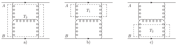
In this appendix we illustrate how a given Feynman diagram contributing to the process (1) in the leading power can be systematically written in the form (27). For concreteness let us consider a two loop diagram where the quarks interact via the exchange of a one rung gluon ladder as in Fig. 12. The important contributions of this diagram come from the regions when all of the exchanged gluons are soft, Fig. 12a or when the gluons attached to the $A$ quark line are soft, while the rest of the gluons carries momenta parallel to the $-$ direction (they belong to jet $B$), Fig. 12b, or when the two gluon lines attached to the $B$ quark line are soft and the other gluons are collinear to the $+$ direction (they belong to jet $A$), Fig. 12c. The possible central soft exchange parts are called tulips. In our case the possible tulips are denoted as $T_{1},T_{2},T_{3}$ in Fig. 12. The garden is defined as a nested set of tulips {$T_{1},\ldots,T_{n}$} such that $T_{i}\subset T_{i+1}$ for $i=1,\ldots,n-1$. In Fig. 12, $\{T_{1}\}$, $\{T_{2}\}$, $\{T_{3}\}$, $\{T_{1},T_{3}\}$, $\{T_{2},T_{3}\}$ are the possible gardens.

For a given tulip we make the soft approximation, consisting of attaching a soft gluon to jet $A$ via the $-$ component of its polarization only and to jet $B$ via the the $+$ component of its polarization. The result of this soft approximation for a given Feynman diagram $F$ corresponding to a tulip $T$ is denoted $S(T)F$. It has obviously the form of Eq. (27). Following the prescription given in Refs. [32] and [4] we write the contribution to a given diagram $F$ in the form

$$F=\sum_{G}(-1)^{n+1}S(T_{1})\ldots\,S(T_{n})\,F+F_{R},$$ (120)

where the sum over inequivalent gardens, as defined bellow, $G$ in Eq. (120) is understood. The meaning of this expression is the following. For a given garden consisting of a set of tulips $\{T_{1},\ldots,T_{n}\}$, we start with the largest tulip $T_{n}$ and make the soft approximation for the gluon lines coming out of it. Then for $T_{n-1}$ we proceed the same way as for $T_{n}$. If some of the lines coming out of $T_{n-1}$ are identical to the ones coming out of $T_{n}$ we leave them untouched. For instance, if we consider a garden $\{T_{2},T_{3}\}$ from Fig. 12, we first perform the soft approximation on tulip $T_{3}$ and then proceed to tulip $T_{2}$. However the lines coming out of $T_{2}$ and $T_{3}$ which attach to the $B$ quark line are identical so when performing $S(T_{2})S(T_{3})F$ we leave these gluon lines out of the game and make soft approximations only on the gluon lines attaching to the ladder’s rung. Two gardens are equivalent if the soft approximation is identical for both of them. $F_{R}$ is defined by Eq. (120). The contribution to $F_{R}$ comes from the integration region where $|\vec{k}|\gtrsim\sqrt{s}$ for all gluons coming out of the central soft part. As a result, the contribution to $F_{R}$ is suppressed by positive powers of $\sqrt{-t}/\sqrt{s}$. Therefore we can ignore the contribution from $F_{R}$ within the accuracy at which we are working.

We can now rewrite Eq. (120), as

$$F=\sum_{T}\left(\sum_{G,T_{n}=T}(-1)^{n+1}\,S(T_{1})\ldots\,S(T_{n-1})\right)S(T)\,F+F_{R}.$$ (121)

This expression is indeed in the form of Eq. (27) since the term $S(T)F$ is of that form and the subtractions $\sum(-1)^{n+1}S(T_{1})\ldots\,S(T_{n-1})$ modify only the soft function $S$ in Eq. (27), but do not alter the form of the equation. We can therefore conclude that the contribution to a given Feynman diagram in leading power can be expressed in the first factorized form given by Eq. (27).

Appendix D Feynman Rules

In Fig. 13, we list the Feynman rules for the lines and the vertices encountered in the text. The double lines are eikonal lines, while the dashed lines represent ghosts. The four vectors $\eta,\,\tilde{\eta}$ are defined in Eqs. (9) and (35), respectively. The conventions for the gluon-ghost and gluon-eikonal vertices (third and second from the bottom of Fig. 13) are the following. We start with a color index of a gluon external to the diagram defining the evolution kernel, see for instance Fig. 8a, then proceed to the gluon internal to the diagram and finally to the ghost/eikonal line in order to assign the color indices of $f_{abc}$. For the three point antighost - gluon - ghost vertex at the bottom of Fig. 13, we start with an antighost (arrow flowing out of the vertex) then proceed to the ghost and finally we reach the gluon line.

Appendix E Origin of Glauber Region

In this appendix we exhibit the origin of the Glauber (Coulomb) region using the two-loop diagram shown in Fig. 14. Consider a situation when the upper gluon loop is a part of $J_{A}$. Momentum $k$ of the exchanged gluon flows through jet lines with momenta $l_{2}=l-k$ and $l_{3}=p_{A}-l-q+k$.

Figure 13: Feynman rules for the eikonal lines, ghost lines and special vertices.

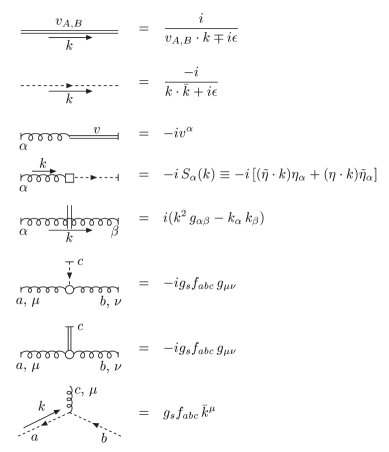
The components of $k$ can be pinched by double poles coming from the denominators of the gluon propagators $k^{2}+i\epsilon$ and $(q-k)^{2}+i\epsilon$. In addition to these pinches, the component $k^{-}$ can be pinched by the singularities of the jet lines $l_{2}$ and $l_{3}$, at values

$$k^{-} = l^{-}-\frac{l_{2\,\perp}^{2}-i\epsilon}{2l_{2}^{+}},$$

$$k^{-} = l^{-}+\frac{l_{3\perp}^{2}-i\epsilon}{2l_{3}^{+}}.$$ (122)

The two poles given by Eq. (E) are located in opposite half planes since in the region considered $l_{2}^{+},l_{3}^{+}>0$. This indicates that we must consider the possibility that the different components of the soft momentum $k$ can scale differently.

Figure 14: Two loop diagram demonstrating the origin of the Glauber (Coulomb) region.

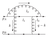
For instance, we can have $k^{+}\sim k_{\perp}\sim\sigma\sqrt{s}$ and $k^{-}\sim\lambda\sqrt{s}$ where $\lambda\ll\sigma\ll 1$. Indeed, the power counting performed in Sec. 3.2 shows that the singularities originating from these regions can produce a logarithmic enhancement. We also note that it is only minus components that are pinched in this way by the lines in $J_{A}$, and plus components by the lines in $J_{B}$.

References

- [1] L.N. Lipatov, in “Perturbative QCD”, ed. A. H. Mueller (World Scientific, Singapore, 1989).
- [2] H. Cheng, T.T. Wu, “Expanding Protons: Scattering at High Energies”, (MIT Press, Cambridge, Massachusetts, 1987).
- [3] J.R. Forshaw, D.A. Ross, Quantum Chromodynamics and the Pomeron, (Cambridge University Press, 1997).
- [4] A. Sen, Phys. Rev. D 27, 2997 (1983).
- [5] T. Jaroszewicz, Acta Phys. Pol. B 11, 965 (1980).
-
[6]
M. Gell-Man, M.L. Goldberger, F.E. Low, E. Marx, F. Zachariasen, Phys. Rev. 133, B145 (1964).
J.C. Polkinghorne, J. Math. Phys. 5, 1491 (1964).
H. Cheng and T.T. Wu, Phys. Rev. 140, B465 (1965). - [7] B.M. McCoy and T.T. Wu, Phys. Rev. D 13, 369 (1976); 379 (1976); 395 (1976); 424 (1976); 484 (1976); 508 (1976).
- [8] A.L. Mason, Nucl. Phys. B 104, 141 (1976); B 117 493 (1976); B 120, 275 (1977).
[9]
L.N. Lipatov, Sov. J. Nucl. Phys. 23, 338 (1976).
E.A. Kuraev, L.N. Lipatov, V.S. Fadin, Sov. Phys. JETP 44, 443 (1976).
E.A. Kuraev, L.N. Lipatov, V.S. Fadin, Sov. Phys. JETP 45, 199 (1977).
Ya. Balitskii, L.N. Lipatov, Sov. J. Nucl. Phys. 28, 822 (1978). - [10] J. Kwiecinski, M. Praszalowicz, Phys. Lett. B 94, 413 (1980).
- [11] J. Bartels, Nucl. Phys. B 151, 293 (1979); B 175, 365 (1980).
- [12] H. Cheng, J. Dickinson, C.Y. Lo, K. Olaussen, P.S. Yeung, Phys. Lett. B 76 129 (1978).
- [13] G.P. Salam, Acta Phys. Pol. B 30, 3679 (1999).
[14]
V.S. Fadin, L.N. Lipatov, Sov. J. Nucl. Phys. 50, 712 (1989); Nucl. Phys. B 477,
767 (1996) [hep-ph/9602287].
V. del Duca, Phys. Rev. D 54, 989 (1996) [hep-ph/9601211]; 4474 (1996) [hep-ph/9604250]. -
[15]
V.S. Fadin, L.N. Lipatov, Nucl. Phys. B 406, 259 (1993).
V.S. Fadin, R. Fiore, A. Quartarolo, Phys. Rev. D 50, 5893 (1994) [hep-ph/9405127].
V.S. Fadin, R. Fiore, M.I. Kotsky, Phys. Lett. B 389, 737 (1996) [hep-ph/9608229].
V. Del Duca, C.R. Schmidt, Phys. Rev. D 59, 074004 (1999) [hep-ph/9810215].
Z. Bern, V. Del Duca, C.R. Schmidt, Phys. Lett. B 445, 168 (1998) [hep-ph/9810409]. -
[16]
V.S. Fadin, R. Fiore, M.I. Kotsky, Phys. Lett. B 359, 181 (1995).
V.S. Fadin, R. Fiore, A. Quartarolo, Phys. Rev. D 53, 2729 (1996).
V.S. Fadin, R. Fiore, Phys. Rev. D 64, 114012 (2001).
J. Blumlein, V. Ravindran, W.L. van Neerven, Phys. Rev. D 58, 091502 (1998) [hep-ph/9806357]. -
[17]
G.P. Korchemsky, Phys. Lett. B 325, 459 (1994).
I.A. Korchemskaya, G.P. Korchemsky, Nucl. Phys. B437, 127 (1995); Phys. Lett. B 387, 346 (1996). - [18] V. del Duca, E.W.N. Glover, JHEP 0110, 035 (2001) [hep-ph/0109028].
- [19] J. Bartels, V.S. Fadin, R. Fiore, The Bootstrap Conditions for the Gluon Reggeization [hep-ph/0307076].
[20]
V.S. Fadin, L.N. Lipatov, Phys. Lett. B 429, 127 (1998) [hep-ph/9802290].
G. Camici, M. Ciafaloni, Phys. Lett. B 412 396 (1997); Erratum B 417 390 (1998) [hep-ph/9707390]; B 430 349 (1998) [hep-ph/9803389]. - [21] A.V. Bogdan, V. del Duca, V.S. Fadin, E.W.N. Glover, JEHP 0203 032, (2002) [hep-ph/0201240].
[22]
C. Anastasiou, E.W.N. Glover, C. Oleari, M.E. Tejeda-Yeomans, Nucl. Phys. B 601, 318 (2001)
[hep-ph/0010212]; B 601, 341 (2001) [hep-ph/0011094]; B 605, 486 (2001) [hep-ph/0101304].
E.W.N. Glover, C. Oleari, M.E. Tejeda-Yeomans, Nucl. Phys. B 605, 467 (2001) [hep-ph/0102201]. -
[23]
L.V. Gribov, E.M. Levin, M.G. Ryskin, Phys. Rept. 100 1 (1983).
A.H. Mueller, J.W. Qiu, Nucl. Phys. B 268 427 (1986).
L. McLerran, R. Venugopalan, Phys. Rev. D 49 2233 (1994); D 49 3352 (1994); D 50 2225 (1994). -
[24]
I. Balitsky, Nucl. Phys. B 463 99 (1996); Phys. Rev.
Lett. 81 2024 (1998) [hep-ph/9807434].
A.H. Mueller, Nucl. Phys. B 558 285 (1999).
Yu.V. Kovchegov, Phys. Rev. D 60 034008 (1999); D 61 074018 (2000).
J. Jalilian-Marian, A. Kovner, L. McLerran, H. Weigert, Nucl. Phys. B 504 415 (1997); Phys. Rev. D 59 014014 (1999); Phys. Rev. D 59 034007 (1999). -
[25]
L.N. Lipatov JETP Lett. 59 596 (1994); Pisma Zh. Eksp. Teor. Fiz. 59 (571) 1994
[hep-th/9311037].
L.D. Faddeev, G.P. Korchemsky, Phys. Lett. B 342 311 (1995) [hep-th/9404173]. - [26] L. Baulieu and D. Zwanziger, Nucl. Phys. B 548 527 (1999) [hep-th/9807024].
- [27] G. Sterman, Phys. Rev. D 17, 2773 (1978).
[28]
G. Sterman, S.B. Libby, Phys. Rev. D 18, 3252 (1978).
G. Sterman, An Introduction to Quantum Field Theory, Cambridge Univ. Press, 1993.
G. Sterman, QCD and Beyond, Proceedings of the Theoretical Advanced Study Institute in Elementary Particle Physics (TASI 95), ed. D.E. Soper (World Scientific, 1996), hep-ph/9606312. -
[29]
J.C. Collins, G. Sterman, Nucl. Phys. B 185 172 (1981).
G.T. Bodwin, S.J. Brodsky, G.P. Lepage, Phys. Rev. Lett. 47 1799 (1981). - [30] S. Coleman, R.E. Norton, Nuovo Cimento 38, 438 (1965).
- [31] A. Sen, Phys. Rev. D 24, 3281 (1981).
- [32] J.C. Collins, D.E. Soper, Nucl. Phys. B 193, 381 (1981).
- [33] G. Grammer, D.R. Yennie, Phys. Rev. D 8, 4332 (1973).
[34]
G. ’t Hooft, Nucl. Phys. B33, 173 (1971).
G. ’t Hooft, M. Veltman, Nucl. Phys. B50, 318 (1972). - [35] C. Becchi, A. Rouet, R. Stora, Commun. Math Phys. 42, 127 (1975); Ann. Phys. 98, 287 (1976).
[36]
H. Kluberg-Stern, J. B. Zuber, Phys. Rev. D 12, 476 (1975); 12, 482 (1975).
N. K. Nielsen, Nucl. Phys. B 101, 173 (1975). - [37] G. Leibbrandt, J. Williams, Nucl. Phys. B 475, 469 (1996).
- [38] G. Leibbrandt, Nucl. Phys. B 64 (Proc. Suppl.), 101 (1998).
- [39] T. Kúcs Gluon Reggeization, In preparation.