Abstract

Evidences and hints, both from the theoretical and experimental side, of exotic baryon resonances with $B=S$, have been with us for the last thirty years. The poor status of the general acceptance of these $Z^{*}$ resonances is partly due to the prejudice against penta-quark baryons and partly due to the opinion that a proof of the existence of exotic states must be rigorous. This can refer to the quality and amount of data gathered, and also to the analytical methods applied in the study of these resonances. It seems then mandatory that all possibilities and aspects be exploited. We do that by analyzing the time delay in $K^{+}N$ scattering, encountering clear signals of the exotic $Z^{*}$ resonances close to the pole values found in partial wave analyses.

1 Introduction

With the advent of the $N^{*}$ program at Jefferson Lab [1] and the forthcoming Japan Hadron Facility [2], the interest in baryon resonances has increased over the last few years. Mysteries of veteran resonances, the hope to find new and ‘missing’ ones and the study of model predictions like the Unitarized Chiral Perturbation Theory [3] are only some topics worth mentioning in this context. But of course, one of the most interesting and exciting subject is the quest to find exotic hadrons [4]. Not all such hadronic states which we would call exotics, can be identified unambiguously. In the mesonic sector this would apply for glueballs, hybrids and mesonic molecules with conventional quantum number assignments. A sure candidate for an exotic meson would be the so-called $J^{PC}$ exotic, which cannot be made up of quark anti-quark pair and appears with quantum numbers, $J^{PC}=0^{--},0^{+-},1^{-+},2^{+-}$ etc. Some candidates have indeed been found [5], but as in the case of exotic baryons they are not yet fully accepted. In the baryonic sector, a clear example of an exotic baryon would be one with its baryon number equal to the strangeness quantum number, i.e $B=S$. Indeed, such a hadronic state would either have to be a composite of five valence quarks, i.e., $q^{4}\bar{s}$ with $q\neq s$, or a $K^{+}N$ molecule i.e. a bound state of hadrons. These resonances are usually called $Z$ or $Z^{*}$ resonances. Evidence for the existence of such resonances dates back to the early 70’ s (see [6, 7] for a collection of references on early $KN$ experiments) and continues in the 80’s ( see the reference list in [8, 9]). This has been accompanied by theoretical predictions mostly in favour of the existence of penta-quarks [10, 11]. The situation is, however, more than confusing as the experimental signals are called ‘pseudoresonances’, ‘doorways’, ‘resonance-like structures’ and ‘resonance-like loops’ (moving counterclockwise in the Argand diagrams). These terms do not carry much physical meaning. We say this because, a resonance is at least theoretically, clearly defined as an unstable state characterized by different quantum numbers. The physical reasons for this caution are also not always clearly stated in the papers. However, in [12] we find the following statement: “Martin and Oades [2] [our reference [13]] interpreted these waves as complicated structures in the unphysical sheet instead of simple resonance poles, because the peaks of the speed plots did not coincide with the peaks of the “resonance”. This is also the case for the three waves obtained in the present paper.” Since we have already done an analysis of time delay (a concept related to speed plots as we shall explain below) [14, 15, 16], the above statement has motivated us to look into the matter more closely. Using the latest $K^{+}N$ scattering data in the form of phase shifts and $T$-matrix solutions [8, 17], we calculate both the time delay and speed plots. We adopt the conservative point of view that we can promote eventually a resonance candidate to a fully accepted member of the resonance spectrum, only if the pole values of the masses found in the partial wave analysis agree with the values of peaks in speed plots and time delay. This restriction is more than one can impose on standard resonances. For example, the $S_{11}$ resonance $N(1535)$ which is claimed to be missing in the speed plots [18] and the $P_{31}$ resonance $\Delta(1910)$ which gives no signal in the time delay plots [14, 15] are both taken as well-established resonances. Hence, our requirement for the confirmation of an exotic $Z^{*}$ resonance is doubly strict.

2 Time delay and speed plots

In this section, we shall discuss the concepts of time delay and speed plots. Though both the methods are useful tools in analyzing resonances, they are different quantities (in certain cases, they differ only by a crucial minus sign) and their origin is also different. Time delay has an intuitive background which we would like to explain. The authors of [19] in a section where they compare Feynman diagrams to electric circuits state: “If it is possible for the intermediate particle to be real, then the process becomes unbounded in space-time and the corresponding amplitude singular”. If this intermediate state (formed for example in two body scattering) is in the $s$-channel and is also a resonance, the singular amplitude can be tamed by a Breit-Wigner form, at least for elementary processes like for example the $e^{+}\,e^{-}\,\rightarrow Z^{0}\rightarrow\,\mu^{+}\,\mu^{-}$ reaction. A similar ‘catastrophe’ can take place with a particle in the $t$-channel if one starts with an unstable particle [20], but this happens because we have violated the requirement that the scattering states be asymptotically free at large distances from the scattering centre. In any case, both reactions are non-localized (‘unbounded’) in space-time. The first case which is of interest for us here, can be visualized as follows: a resonance is produced on-shell at a space-time point $(t_{1},x_{1})$, it propagates for some time and decays at a space-time point $(t_{2},x_{2})$. Certainly, the reaction is time delayed (by an amount $\Delta t=t_{2}-t_{1}$) and the time delay has to be positive. This picture is qualitatively model independent, as it does not depend on the form of the analytical tool by which the resonance is described (Breit-Wigner, a modified version of the same, etc.) and this makes it useful for broad hadronic states. Eisenbud and Wigner [21, 22, 23] found a way to evaluate this time delay, $\Delta t$, from the phase shift $\delta$ as,

$$\Delta t=2\hbar{d\delta\over dE}\,.$$ (1)

It can also be evaluated from the $S$ matrix, generalizing at the same time, the time delay in elastic channels (1) to an arbitrary reaction $i\to j$ as, [24]

$$\Delta t_{ij}=\Re e\biggl{[}-i\hbar(S_{ij})^{-1}{dS_{ij}\over dE}\biggr{]}\,$$ (2)

with the identification, $\Delta t_{ii}=\Delta t$. Defining the $T$ matrix as

$$S_{kj}=\delta_{kj}+2iT_{kj}\,,$$ (3)

with

$$T_{kj}=\Re eT_{kj}+i\Im mT_{kj}$$ (4)

we get

$$S^{*}_{ii}S_{ii}\,\Delta t_{ii}=2\hbar\biggl{[}{d\Re eT_{ii}\over dE}+2\Re eT_{ii}{d\Im mT_{ii}\over dE}-2\Im mT_{ii}{d\Re eT_{ii}\over dE}\biggr{]}.$$ (5)

Parameterizing a general $T$-matrix for the elastic channel in the presence of non-zero inelasticities, through the phase shift $\delta$ and the energy dependent inelasticity parameter $\eta$ as,

$$T={\eta e^{2i\delta}-1\over 2i},\,\,\,\,\,\,0<\eta\leq 1$$ (6)

one can show that $\Delta t$ is given by (1) even if $\eta\neq 1$. Time delay can be positive as well as negative. A big positive peak is expected within the kinematical vicinity of a resonance. Large regions of negative time delay can occur due to the opening of new channels or due to a repulsive interaction, or in the presence of several resonances even with all inelasticities zero [25]. Sometimes one hears/reads statements like ‘the phase shift has to change sharply to indicate a resonance’ or ‘a phase motion indicates a resonance’. Very often it is stated that the phase shift has to increase by an odd multiple of $\pi/2$ while passing through the resonance region. Whereas the first statement is not precise enough, the second one is model dependent. Indeed, it originates from

$$\delta_{res}(E)\simeq\tan^{-1}\biggl{[}{\Gamma/2\over E_{R}-E}\biggr{]}$$ (7)

which gives a Breit-Wigner form, namely,

$${d\delta\over dE}={\Gamma\over 2}{1\over(E_{R}-E)^{2}+\Gamma^{2}/4}\,.$$ (8)

The reason behind both the above statements is actually the time delay, which is a model independent analytical justification of both of them. Moreover, as evident from the last equation, $\Delta t(E)$ is essentially the spectral density used to calculate survival probabilities [26] which carries some importance if $\Delta t$ is not a Breit-Wigner.

The concept of time delay and its connection to resonances is well documented in many papers and found its entry in many textbooks. For a complete list of references we refer the reader to [16]. Here we remark that an operator for time delay has been found by Lippmann in [27]. Time delay can also be applied to steady-state solutions of Maxwell equations for the total reflection case [28], to chaotic scattering [29] and to transport theory in heavy ion collision [30], all showing the wide applicability of $\Delta t$. Before applying it to $KN$ scattering, we would like to compare it with speed plots.

The speed plot is defined through

$$SP(E)=\biggl{|}{dT\over dE}\biggr{|}\,.$$ (9)

Its first appearance is less clear than in the case of time delay. It probably stems from the Argand diagrams, as it describes the speed at which the curve in the Argand diagram is traversed with $E$ playing the role of the affine parameter. Using equation (6) we get,

$$SP(E)=\sqrt{\eta^{2}\biggl{(}{d\delta\over dE}\biggr{)}^{2}+{1\over 4}\biggl{(}{d\eta\over dE}\biggr{)}^{2}}$$ (10)

which shows that if $\eta=1$, $SP(E)=|\Delta t|/2$. Even in this case, a speed plot is not the same as a time delay plot, since large negative regions in the time delay plots will become positive peaks in the speed plots. This fact is unfortunate, since only positive peaks in time delay indicate a resonance. For example, the negative dips in time delay in the $S_{01}$, $D_{03}$ and $D_{15}$ partial waves in Fig. 2, appear as positive bumps in the speed plots. In the $P_{01}$ and $P_{13}$ partial waves, one can see that the resonant peak in the speed plot is broadened as compared to the time delay peak which is narrower due to the presence of negative time delay. That time delay can be negative even in the case of $\eta=1$ was noticed already by Wigner [21] and an explicit example of this is given in [25]. If $\eta\neq 1$, the situation described above still persists, but then, even the proportionality, $SP(E)=|\Delta t|/2$ vanishes. Indeed, we could have done our analysis without using the speed plots. However, since two earlier references used it in analyzing the $KN$ data, we would like to make a correct comparison with their results.

3 Time delay, speed plots and resonances in $K^{+}N$ scattering

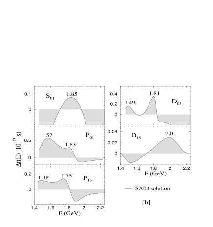
Figure 1: (a) Real (dashed lines) and imaginary (solid lines) parts of the $T$-matrix solutions [8] as compared to the single energy values the real part (filled triangles) and imaginary part (open triangles) for various partial waves in $K^{+}N$ scattering (b) time delay evaluated using the $T$-matrix solutions (shown in (a))

Since the $T$-matrix (see Fig. 1) solutions found in [8], agree very well in the crucial cases with the single energy values of the T-matrix and phase shifts, we calculate, with the exception of the $S_{01}$ partial wave (where we also use the single energy values), the time delay and speed plots from these solutions. The results for time delay are presented in Fig. 1 and for the speed plots in Fig. 2, where for comparison we have included the time delay results too.

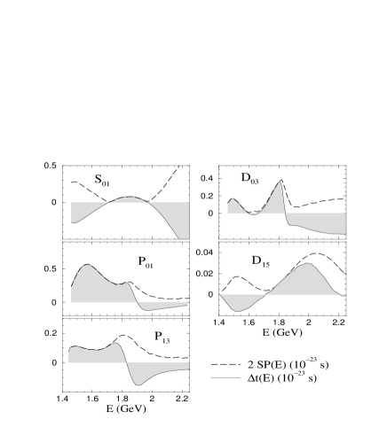
Figure 2: Comparison of time delay and speed plots in various partial waves of $K^{+}N$ scattering.

It appeared to us that in the case of the partial wave, $S_{01}$, the agreement between the solution and single energy values is not as good as in the other partial waves. We therefore decided to calculate $\Delta t$ from the solution as well as from a fit made to the data points. These results can be found in Fig. 3.

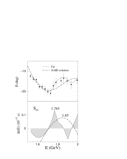
Figure 3: Single energy values of phase shifts (filled circles) and time delay evaluated from a fit (solid line) to these phase shifts and from the solution (dashed line) as in Fig. 1, for the $S_{01}$ partial wave in $K^{+}N$ scattering.

The T-matrix poles found in [8] are: $P_{01}(1831)$, $P_{13}(1811)$, $D_{03}(1788)$ and $D_{15}(2074)$. Comparing these values with the peak positions in the time delay plots for the corresponding partial waves, we see that the agreement is very good. We do not expect a complete agreement here between pole values and time delay peak values as this also does not occur in the conventional cases of pion-nucleon resonances [14, 15]. As evident from the theoretical example in [25], the mass parameters appear shifted in time delay plots due to overlapping effects of several resonances. The agreement of the peak values in the speed plot with the above mentioned pole values is also excellent. Hence we can ask ourselves the question: ‘what other objection prevents us from accepting the four $Z^{*}$ exotic resonances’? Note that the pole values (and of course the corresponding peaks in our plots) for $P_{01}$, $P_{13}$ and $D_{03}$ display a certain regularity. The three pole values are very close to the $K^{*}(892)N$ threshold. This is, however, a well known phenomenon. For instance, there are several well established pion-nucleon resonances close to the $\rho N$ threshold. Theoretically, this phenomenon has been known since the early 60’s [32]. In [31] (mentioned also in [9]) it is speculated that the signals for the resonances could be faked by a $K^{*}$-box diagram (essentially the pion exchange diagrams $KN\to K^{*}N$ and $K^{*}N\to KN$ glued together). In principle, we could address a similar question for higher lying pion-nucleon resonances by replacing the $K^{*}$-box with a $\rho$-box, i.e. replacing the $K$ by $\pi$ and $K^{*}$ by $\rho$.

Furthermore, in [33] the very same $K^{*}$-box was used as an input to dynamically generate the $Z^{*}$ resonances. The predicted $Z^{*}$ resonances in [33] are $S_{01}$ and $D_{03}$ around $1830$ MeV. The model in [33] has been put to a partial test in [6] which analyzes data by using this model. The speed plots in [6] agree very well with our results. This actually means that, had the authors of [6] evaluated time delay, their results would have also agreed with ours. It is important to note that our results for the time delay indicate that the signal for a particular $Z^{*}$ resonance is a genuine one. To understand this, we have to go back to the pion-nucleon resonances [14]. In [14] it was found that the opening of a new channel drives the positive time delay in the elastic channel into regions of negative time delay. It actually starts becoming negative around the threshold of a new channel, very often interfering with the positive signal of the resonance itself. It was found that in more than one case, this leaves only a small positive peak (due to the resonance). That this is bound to happen is also clear from the connection of time delay with density of states (see the discussion in [14] and [16]). A ‘removal’ of the initial states due to inelasticity makes the time delay negative. The probability of this inelastic channel usually decreases with energy. Hence, in the absence of a resonance, for the $K^{*}$-box diagram, we would expect only a negative time delay around $K^{*}(892)N$ threshold becoming a positive continuum (due to the off-shell box diagram) at much higher energies. We do not find such a behaviour in our time delay analysis, but rather positive peaks around $1830$ MeV, followed by regions of negative time delay. This is identical to the case of standard resonances in pion-nucleon scattering. Note that this conclusion would be impossible to make using solely speed plots.

As mentioned in the Introduction, the rigor that one wishes to apply to exotics, demands that pole values be equal to the peak values of time delay and speed plots; a consistency not always encountered in the standard hadron resonances. Hence, we shall only briefly discuss the other peaks found in our plots. The peak in $S_{01}$ at $1850$ MeV (or $1765$ MeV in Fig. 3) was interpreted in [33, 6] as a resonance. In [11] a resonance at $(1710)$ MeV in the $S_{01}$ partial wave was predicted. The time delay peaks at $1.5$ GeV, in the $P_{01}$, $P_{13}$ and $D_{03}$ partial waves, also have a certain regularity. Some recent calculations [34] made within the collective quantization scheme for chiral solitons predict a penta-quark state, essentially an exotic $Z^{*}$ around mass 1570 MeV. In yet another chiral soliton model [35], a $Z^{*}$ at $1530$ MeV was predicted. In ref. [36], the authors show that the $pp\rightarrow n\Sigma^{+}K^{+}$ reaction provides optimal conditions to detect the $Z^{*}$ if its mass is located around 1.5 GeV. Finally, we also note that in a much older analysis [12], one can see a clear peak around 1550 MeV in the speed plots of Fig. 3, although the authors do not explicitly mention this fact in their table of resonance parameters. These predictions taken along with our findings of the low energy peaks in time delay could possibly hint towards the existence of a low mass $Z^{*}$ in addition to the one around 1850 MeV.

4 Conclusions

The last entry of the $Z^{*}$ exotic resonances into the Particle Data Group compilation was in 1992 [37]. In the same edition, it was remarked that it might take twenty years before the issue of the existence of the $Z^{*}$ resonances is settled. One might think that this is due to the lack of data. However, this is not the case. The first data sets, date back from 1969/1970, followed by several others in the 70’s and 80’s with the last one in 1982. The latest analysis is not restricted to a single data set, but includes many of them [8]. Hence we cannot blame the lack of data if we are reluctant to decide the fate of the $Z^{*}$’s.

In [12] it was remarked that: “It was found that both data showed reasonable agreement with each other but the agreement with the published analyses were not satisfactory.” Reference [12] is the same which does not find an agreement between pole value and values found in speed plots (similar to [13]). Hence an internal consistency of data and analysis is required. As far as the existence of resonances is concerned, this can be done e.g. by checking if the pole values agree with values obtained from time delay method and speed plots. We emphasize here the time delay method since in contrast to speed plots the resonance region in the time delay plots has to be positive . As remarked in the Introduction, this is more than we have for some of the four-star pion-nucleon resonances. Our analysis reveals that the pole values found in [8] are in excellent agreement with the values for the masses found in time delay and speed plots.

From a collection of data set progressing in time one would expect certain improvements, here with regard to resonance extraction. In one of the early analysis of $KN$ scattering, it was demonstrated that ‘polarization measurements would be very helpful in demonstrating the existence of these resonances’. At that time, only one polarization measurement existed. However, this suggestion was picked up later in a series of experiments (see [8] for a list of references) and included in the analysis in [8].

Finally, from different data and different analyses, one would demand a certain consistency among each other . Here comes a small surprise. Reference [6] analyzed the early data from 1970’s using at the same time a theoretical input to distinguish between solutions. This input is the model in reference [33] discussed in the previous section. Fig. 3 in [6] displays the speed plots for $S_{01}$, $P_{01}$ and $D_{03}$ partial waves in $KN$ collisions calculated in 1973. Their form resembles very much our results for speed plots depicted in Fig. 2. More importantly, the peak values of the speed plots in [6] are in excellent agreement with ours, though our result is based on a bigger data set and as far as we can say with lesser theoretical input. Yet another surprise comes, when we realize that the speed plot peaks in the $P_{13}$ and $D_{03}$ partial waves in [12] are around $1825$ MeV.

To summarize, we can say that, we laid certain restrictions for the existence of the exotic $Z^{*}$ resonances. Within these restrictions the results were found to be consistent, hinting towards the existence of these resonances. We think that these hints should be taken seriously.

Acknowledgements
We thank Juan Carlos Sanabria for stimulating discussions on exotic baryons.

Note added after publication: After this work was published, we became aware of the work in [38, 39, 40], where excellent experimental evidence for an exotic $S=+1$ baryon, with mass around 1.54 GeV was reported. We speculate that it can be identified with the $P_{01}(1.57)$ of the present work.

References

- [1] V. D. Burkert 2002 “Status of the program at Jefferson Lab”, Preprint hep-ph/0210321
- [2] R. S. Hayano 1999 Nucl. Phys. A 655 369
- [3] E. Oset 2002 “Unitarized chiral perturbation theory of hadrons”, nucl-th/0211077; talk given at PANIC 2002, Osaka, October 2002; D. Jido, E. Oset and A. Ramos 2002 Phys. Rev. C 66 055203; A. Ramos, E. Oset and C. Bennhold 2002 Phys. Rev. Lett. 89 252001; E. Oset, T. Inoue, M. J. Vicente Vacas, A. Ramos and C. Bennhold 2002 “Chiral unitary approach to hadron spectroscopy”, nucl-th/0209018; talk given at the workshop on partial wave analysis of meson and baryon systems, Pittsburgh, June 2002; T. Inoue, E. Oset and M. J. Vicente Vacas 2002 Phys. Rev. C 65 035204.
- [4] F. Close 1997 Nature 389 230; S. U. Chung 1997 Nucl. Phys. Proc. Suppl. 56 234; G. S. Adams et al. 2000 Nucl. Phys. A 680 335; M. Gerber and M. Nowakowski 1992 Nucl. Phys. A 548 681; C. J. Burden and M. A. Pichowsky 2002 Few Body Syst. 32 119; T. Barnes and E. S. Swanson 1994 Phys. Rev. C 49 1166.
- [5] D. R. Thompson et al. 1997 Phys. Rev. Lett. 79 1630; A. Abele et al. 1998 Phys. Lett. B 423 175
- [6] R. Aaron, M. Rich, W. L. Hogan and Y. N. Srivastava 1973 Phys. Rev. D 7 1401
- [7] S. Kato et al. 1970 Phys. Rev. Lett. 24 615
- [8] J. S. Hyslop, R. A. Arndt, L. D. Roper and R. L. Workman 1992 Phys. Rev. D 46 961
- [9] R. A. Arndt and L. D. Roper 1985 Phys. Rev. D 31 2230
- [10] T. DeGrand, R. L. Jaffe, K. Johnson and J. Kiskis 1975 Phys. Rev. D 12 2060; R. J. Jaffe and F. E. Low 1979 Phys. Rev. D 19 2105
- [11] C. Roiesnol 1979 Phys. Rev. D 20 1656
- [12] K. Nakajima et al. 1982 Phys. Lett. B 122 80
- [13] B. Martin and G. C. Oades 1980 in IVth International conference on baryon resonances, Toronto
- [14] N. G. Kelkar 2003 J. Phys. G: Nucl. Part. Phys. 29 L1 (Preprint, hep-ph/0205188).
- [15] N. G. Kelkar, Marek Nowakowski, K. P. Khemchandani and S. R. Jain 2002 Preprint hep-ph/0208197
- [16] N. G. Kelkar, Marek Nowakowski and K. P. Khemchandani 2002 “Collision times in and scatterings and spectroscopy of meson resonances” Nucl. Phys. A (in press).
- [17] Single energy values of phase shifts can be obtained from the SAID program made available on internet (URL: http://gwdac.phys.gwu.edu) by R. A. Arndt et al. To access it by telnet, link to gwdac.phys.gwu.edu with ‘LOGIN:said’. Password is not required.
- [18] G. Höhler 1998 Newsletter 14 168
- [19] J. D. Bjorken and S. D. Drell 1964 Relativistic Quantum Fields (McGraw-Hill, New York)
- [20] M. Nowakowski and A. Pilaftsis 1993 Z. Phys. C 60 121
- [21] E. P Wigner 1955 Phys. Rev. 98 145
- [22] E. P. Wigner and L. Eisenbud 1947 Phys. Rev. 72 29
- [23] L. Eisenbud 1948 (dissertation, Princeton (unpublished))
- [24] F. T. Smith 1960 Phys. Rev. 118 349; ibid 1963 Phys. Rev. 130 394
- [25] N. R. Lipshutz 1969 Phys. Rev. 181 1972
- [26] M. Nowakowski 1999 Int. J. Mod. Phys. A 14 589 and references therein; J. Bogdanowicz, M. Pindor and R. Raczka 1995 Found. Phys. 25 833
- [27] B. A. Lippmann 1966 Phys. Rev. 151 1023
- [28] J. L. Agudin 1968 Phys. Rev. 171 1385
- [29] P. W. Brouwer, K. M. Frahm and C. W. J. Beenakker 1997 Phys. Rev. Lett. 25 4737; Y. V. Fyodorov and H.-J. Sommers 1996 Phys. Rev. Lett. 76 4709
- [30] P. Danielewicz and S. Pratt 1996 Phys. Rev. C 53 249; A. B. Larionov et al. 2001 Preprint nucl-th/0107031; S. Leupold 2001 Nucl. Phys. A 695 377; C. David, C. Hartnack and J. Aichelin 1999 Nucl. Phys. A 650 358
- [31] I. M. Narodetskii and Y. A. Simonov 1978 Sov. J. Phys. 28 698
- [32] J. S. Ball and W. R. Frazer 1961 Phys. Rev. Lett. 7 204
- [33] R. Aaron, R. D. Amado and R. R. Silbar 1970 Phys. Rev. Lett. 26 407; the conventional pion-nucleon resonances have been treated in R. Aaron and R. D. Amado 1971 Phys. Rev. Lett. 27 1316
- [34] H. Weigel 2002 AIP Conf. Proc. 549 271, hep-ph/0006191; it ibid 1998 Eur. Phys. J A 2 391
- [35] D. Diakonov and M. Polyakov 1997 Z. Phys. A 359 305
- [36] M. V. Polyakov, A. Sibirtsev, K. Tsushima, W. Cassing and K. Goeke 2000 Eur. Phys. J A 9 115
- [37] K. Hikasa et al. (Particle Data Group) 1992 Phys. Rev. D 45 S1
- [38] T. Nakano et al. 2003, Phys. Rev. Lett. 91 012002.
- [39] S. Stepayan et al. (CLAS collaboration), Preprint: hep-ex/0307018.
- [40] V. V. Barmin et al. (DIANA collaboration), Preprint: hep-ex/0304040.