We study the process $e^{+}e^{-}\to e^{+}e^{-}\not{\!\!E}$ at a high-energy $e^{+}e^{-}$ collider, where the missing energy arises from the radiation of Kaluza-Klein gravitons in a model with large extra dimensions. It is shown that at a high-energy linear collider, this process can not only confirm the signature of such theories but can also sometimes be comparable in effectiveness to the commonly discussed channel $e^{+}e^{-}\to\gamma\not{\!\!E}$, especially for a large number of extra dimensions and with polarized beams. We also suggest some ways of distinguishing the signals of a graviton tower from other types of new physics signals by combining data on our suggested channel with those on the photon-graviton channel.

PACS No. 04.50.+h, 11.10.Kk, 11.25.Mj, 12.60.-i, 13.88.+e

1 Introduction

It is a matter of common belief in the high-energy physics community that there must be physics beyond the Standard Model (SM) around the TeV scale. This belief is founded in the fact that some of the parameters of the SM can be made stable against quantum corrections only by invoking new physics at the TeV scale. With this in mind, an enormous international effort is being poured into the construction of the 14-TeV LHC at CERN, which is expected to run by 2008 and come up with signals for new physics. However, as the LHC is a hadronic machine, it is unlikely to yield signals which are unequivocal as to the underlying theory. It is therefore widely deemed necessary to build a high-energy $e^{+}e^{-}$ collider to confirm the nature and detailed properties of this new physics.

A high-energy $e^{+}e^{-}$ collider operating in the range 500 GeV to a few TeV must be of the linac type to avoid large synchrotron radiation losses. Such a machine would require a very high luminosity in order to be competitive with other accelerators. This is, in fact, an essential feature of the design[1] of proposed linear colliders. The relatively clean environment of an $e^{+}e^{-}$ collider allows the complete reconstruction of individual events, making it possible to carry out precision tests of new physics. Moreover, one has the facility of polarizing the beams, which can play a significant role in background elimination. It is also possible to run such a machine in the $e^{-}e^{-}$, $e\gamma$ and $\gamma\gamma$ modes. In this paper we consider the possibility of using a high energy $e^{+}e^{-}$ collider to detect signatures of low-scale quantum gravity in a model with large extra dimensions. In particular, we focus on Bhabha scattering with radiated gravitons.

One of the most exciting theoretical developments of recent years has been the idea that there could be one or more extra spatial dimensions and the observable Universe could be confined to a four-dimensional hypersurface in a higher-dimensional ‘bulk’ spacetime[2]. Such ideas, which can be motivated by superstring theories, give rise to elegant solutions[3] to the well-known gauge hierarchy problem of high energy physics, which is just the instability against quantum corrections mentioned above. What is even more interesting, perhaps, is the suggestion[4, 5] that there could be observable signals of quantum gravity at current and future accelerator experiments, and this possibility has spawned a vast and increasing body of work over the past five years. This relatively new set of ideas, commonly dubbed ‘Brane World Phenomenology’, bases itself on two main principles: the concept of hidden compact dimensions and the string-theoretic idea of $D_{p}$-branes. The simplest brane-world scenario is the so-called Arkani-Hamed—Dimopoulos—Dvali (ADD) model[3], in which there are $d$ extra spatial dimensions, compactified on a $d$-torus of radius $R_{c}$ each way. Together with the four canonical Minkowski dimensions, this constitutes the ‘bulk’ spacetime. In this scenario the radius $R_{c}$ of the extra dimensions can be as large as a quarter of a millimeter[6]. However, the SM fields are confined to a four-dimensional slice of spacetime, with thickness not more than $10^{-17}$ cm, which is called the ‘brane’. If the ADD model is embedded in a string-theoretic framework, the ‘brane’ is, in fact a $D_{3}$-brane, i.e. a 3+1 dimensional hypersurface on which the ends of open strings are confined[7]. However, it is not absolutely essential to embed the model in a string theory, and the word ‘brane’ or ‘wall’ is then used simply to denote the hypersurface (or thin slice) where the SM fields are confined. A crucial feature of this model is that gravity, which is a property of spacetime itself, is free to propagate in the bulk. As a result

• Planck’s constant in the bulk $M_{S}$, identified with the ‘string scale’, and fixed by the string tension $\alpha^{\prime}$, is related to Planck’s constant on the brane $M_{P}$ ($\simeq~{}1.2\times 10^{19}$ GeV) by

  $$(M_{S})^{2+d}=(4\pi)^{d/2}~{}\Gamma(d/2)~{}M_{P}^{2}~{}(R_{c})^{-d}$$ (1)

  which means that for $R_{c}\sim 0.2$ mm, it is possible to have $M_{S}$ as low as a TeV for $d\geq 2$. (The normalization of reference [5] has been adopted here). This solves the gauge hierarchy problem simply by bringing down the scale of new physics (i.e. strong gravity in this case) to about a TeV and thereby providing a natural cut-off to the SM, since the string scale $M_{S}$ now controls graviton-induced processes on the brane.

• There are a huge number of massive Kaluza-Klein excitations of the (bulk) graviton field on the brane, with masses $m_{n}=n/R_{c}$, and these collectively produce gravitational excitations of electroweak strength, which may be observable at current experiments and those planned in the near future[8].

It is only fair to mention that a major drawback of the ADD model is that it creates a new hierarchy between the ‘string scale’ $M_{s}\sim 1$ TeV and the size of the extra dimensions $R_{c}^{-1}\sim 1$ $\mu$eV. In fact, the huge size of the extra dimensions (compared to the Planck length) is not stable under quantum corrections, which tend to shrink it down until $M_{s}\sim R_{c}^{-1}\sim M_{P}\sim 10^{19}$ GeV, at which stage the original hierarchy problem is reinstated. Nevertheless, there are several variants of the ADD model which address this problem in various ways, and some of these ideas may not be far from the truth. From a phenomenological point of view, it is, therefore, reasonable to postpone addressing the stability issue, and proceed to study the minimal ADD model and its consequences for experiment.

The experimental consequences of ADD gravity have been mainly studied in the context of of ($a$) real graviton emission and ($b$) virtual graviton exchange. In the former case the final state gravitons in the ADD model are ‘invisible’, escaping the detector because of their feeble individual interactions ($\sim M_{P}^{-1}$) with matter. The final state, involving missing energy due to gravitons, will be built up by making an incoherent sum over the tower of graviton modes. In the case of virtual gravitons, the final state is built up by making a coherent sum. In either case, it may be shown[4, 5] that, after summing, the Planck mass $M_{P}$ cancels out of the cross-section, leaving an interaction of near-electroweak strength.

At an $e^{+}e^{-}$ collider, the most-frequently discussed[4, 9, 10] signal for ADD gravitons is the process $e^{+}e^{-}\to\gamma G_{n}$, where $G_{n}$ is the $n$th Kaluza-Klein excitation of the graviton field. This process leads to single photon events with missing energy and momentum, and is expected to be among the earliest signals of ADD gravity at an $e^{+}e^{-}$ collider. In addition, the process $e^{+}e^{-}\to\mu^{+}\mu^{-}G_{n}$ has also been studied[11]. In this work, we have studied the process

$$e^{+}e^{-}\to e^{+}e^{-}G_{n}$$

which is simply Bhabha scattering with a radiated graviton. The final state would contain an electron-positron pair with substantial missing energy. The reasons for taking up a study of this process are as follows.

• At an $e^{+}e^{-}$ collider, final states with an $e^{+}e^{-}$ pair will be one of the first things to be analyzed, since this is needed for beam calibration[1]. Among such states, it should be a simple matter to select events with large missing energy as well.

• Unlike $e^{+}e^{-}\to\mu^{+}\mu^{-}G_{n}$, this process does not suffer from large $s$-channel suppression, especially if one considers final state electrons (positrons) in relatively forward (backward) directions.

• Taken in conjunction with the process $e^{+}e^{-}\to\gamma G_{n}$, this process could help to distinguish signals of the ADD scenario from other physics models beyond the SM. This is elaborated in the subsequent discussions.

• In some ways, as we shall see, this process has signatures more distinct from other new physics effects than $e^{+}e^{-}\to\gamma G_{n}$.

In the following section we describe the salient features of our calculation of the signal process. Backgrounds and some strategies for their elimination are discussed in section 3. Section 4 contains the results of our numerical analysis. In section 5 we discuss how this process can be used to pinpoint the model if signatures of the suggested type are indeed observed. We summarize and conclude in the final section.

2 The Process $e^{+}e^{-}\to e^{+}e^{-}G_{n}$

As gravity couples to the energy-momentum tensor, each component of the tower of ADD gravitons couples to all SM fields, as well as to each SM interaction vertex. The relevant Feynman rules can be found, for example, in Refs.[4, 5]. Using these, it can be shown that the process $e^{+}e^{-}\to e^{+}e^{-}G_{n}$ is driven, at tree-level, by 28 Feynman diagrams. Some representative diagrams are shown in Fig. 1, which are obtained by ‘dressing’ an $s$-channel process $e^{+}e^{-}\to e^{+}e^{-}$ with graviton radiation. Fig. 1($a$) represents a graviton emission from one of the external electron legs; there will be 4 such diagrams with the graviton emitted from each leg in turn. Fig. 1($b$) represents a graviton emission from the gauge boson propagator. Fig. 1($c$) represents a graviton emission from one vertex; there will be another such with graviton emission from the other vertex. Thus Fig. 1 encompasses 14 diagrams, 7 each with $Z$ and photon exchanges. In addition, there will be another set of 14 diagrams with the $\gamma,Z$ exchange in the $t$-channel, making 28 diagrams in all. This latter set is absent in the case of $e^{+}e^{-}\to\mu^{+}\mu^{-}G_{n}$.

Figure 1. Representative Feynman diagrams for the process $e^{+}e^{-}\to e^{+}e^{-}G_{n}$.

Considering the process

$$e^{-}(k_{1},\lambda_{1})~{}e^{+}(k_{2},\lambda_{2})\to G_{n}(p_{1})~{}e^{+}(p_{2})~{}e^{-}(p_{3})$$

with a single Kaluza-Klein mode $G_{n}(p_{1})$ in the final state, we obtain the unpolarized cross-section

$$\sigma(m_{n})=\frac{1}{2s}\int\frac{d^{3}\vec{p_{1}}}{(2\pi)^{3}~{}2E_{1}}~{}\frac{d^{3}\vec{p_{2}}}{(2\pi)^{3}~{}2E_{2}}~{}\frac{d^{3}\vec{p_{3}}}{(2\pi)^{3}~{}2E_{3}}~{}\delta^{4}(k_{1}+k_{2}-p_{1}-p_{2}-p_{3})~{}~{}\frac{1}{4}\sum_{\lambda_{1},\lambda_{2}}|M_{n}(\lambda_{1},\lambda_{2})|^{2}$$ (2)

where the final state helicities are summed over. This cross-section is a function of the mass $m_{n}$ of the graviton excitation.

The squared matrix element $|M_{n}(\lambda_{1},\lambda_{2})|^{2}$ for the process can be written as the sum

$$|M_{n}(\lambda_{1},\lambda_{2})|^{2}=\left|\sum_{i=1}^{28}M_{n}^{(i)}(\lambda_{1},\lambda_{2})\right|^{2}$$ (3)

where $|M_{n}^{(i)}(\lambda_{1},\lambda_{2})|^{2}$ represents the squared helicity amplitude arising from the $i$th diagram. In our calculation, we make use of the helicity amplitude technique to write down amplitudes for all these 28 diagrams and evaluate the individual terms in the above sum using the subroutine HELAS[12].

Recalling that the observed final state, namely, $e^{+}e^{-}$ plus missing energy, consists of an incoherent sum over the tower of graviton modes, we get

$$\sigma(e^{+}e^{-}\to e^{+}e^{-}+\not{\!\!E}) = \sum_{n}\sigma(m_{n})$$ (4)

$$\simeq \int_{0}^{\sqrt{s}}dm~{}\rho(m)~{}\sigma(m)$$

approximating the discrete (but closely-spaced) tower of states by a continuum. The density of states is given by[5]

$$\rho(m)=\frac{2~{}R_{c}^{d}~{}m^{d-1}}{(4\pi)^{d/2}~{}\Gamma(d/2)}\ ,$$ (5)

and the integration is cut off at the kinematic limit $\sqrt{s}$.

As the calculation, even using HELAS, is long and cumbersome, some checks on the numerical results are called for. The most useful check is provided by the Ward identities arising from general coordinate invariance, which constitute an essential feature of any theory involving gravity. We can write the amplitude for the emission of any graviton in the form

$$M_{n}(\lambda_{1},\lambda_{2})=T^{\mu\nu}(\lambda_{1},\lambda_{2})~{}\epsilon^{(n)*}_{\mu\nu}(p_{1})$$ (6)

where $\epsilon^{(n)}_{\mu\nu}(p_{1})$ is the polarization tensor for the $n$th (massive) graviton mode. The tensor $T^{\mu\nu}(\lambda_{1},\lambda_{2})$ is the same for every mode, including the massless mode $\epsilon^{(0)}_{\mu\nu}(p_{1})$, which is the usual graviton of four-dimensional Einstein gravity. This must now satisfy the Ward identities

$$p_{1}^{\mu}T_{\mu\nu}(\lambda_{1},\lambda_{2})=p_{1}^{\nu}T_{\mu\nu}(\lambda_{1},\lambda_{2})=0\ ,$$ (7)

where we note that

$$T^{\mu\nu}(\lambda_{1},\lambda_{2})=\sum_{i=1}^{28}T_{i}^{\mu\nu}(\lambda_{1},\lambda_{2})$$ (8)

with $i$ indicating the $i$th diagram, as above. The consistency check therefore requires a perfect cancellation, for each choice of $\lambda_{1}$ and $\lambda_{2}$, between all such terms, which is highly sensitive to errors in signs and factors. We have also checked that if only the $s$-channel results are taken our numerical results are in close agreement with those of Ref.[11], and this, of course, implies that the $t$-channel contributions can be easily checked using crossing symmetry.

In our numerical analysis of this problem, we have also considered diagrams mediated by gravitons in place of $\gamma,Z$. Such diagrams, in fact, are of the same order in perturbation theory after summation over the graviton propagators, but it turns out that the contributions are very small — typically less than 1% for experimentally-allowed values of $M_{S}$ — due to the smallness of the effective graviton coupling after summation.

It is also worth mentioning that contributions due to graviscalars in the ADD model can also be neglected. It can be shown[5] that diagrams with graviscalars coupling to external fermion legs and vertices undergo large cancellations and the final contribution is proportional to the electron mass. This leaves only the diagrams with graviscalars emitted from the massive $Z$-propagator, which is again suppressed at high energies by a factor of $M_{Z}^{2}/s$ compared to the gravitensor contributions, the latter being jacked up by derivative couplings.

3 Background Elimination

The actual signal for the process considered in the previous section consists of a hard electron and a hard positron, with substantial missing energy. The SM backgrounds arise from all processes of the form $e^{+}e^{-}\to e^{+}e^{-}\nu\bar{\nu}$, where the neutrinos can be of any flavor. At the lowest order, there are 96 Feynman diagrams which give rise to this final state. Some of the principal sub-processes are listed below.

$$e^{+}e^{-} \to e^{\pm}W^{\mp}\nu_{e}^{\!\!\!\!\!\!(-)}\to e^{+}e^{-}\nu_{e}\bar{\nu}_{e}$$

$$e^{+}e^{-} \to e^{+}e^{-}Z\to e^{+}e^{-}(\nu\bar{\nu})$$

$$e^{+}e^{-} \to \nu_{e}\bar{\nu}_{e}Z\to\nu_{e}\bar{\nu}_{e}(e^{+}e^{-})$$

$$e^{+}e^{-} \to W^{+}W^{-}\to(e^{+}\nu_{e})(e^{-}\bar{\nu}_{e})$$

$$e^{+}e^{-} \to ZZ\to(e^{+}e^{-})(\nu\bar{\nu})$$

$$e^{+}e^{-} \to \gamma^{*}Z\to(e^{+}e^{-})(\nu\bar{\nu})$$ (9)

Of course, for every process with real $W/Z$, there will also be many diagrams with off-shell particles. Taken together, all these diagrams constitute a formidable background to the suggested signal. A judiciously chosen set of kinematic cuts, however, enable us to reduce these backgrounds enormously. For example, diagrams with the neutrino pair (missing energy) arising from a real $Z$ boson can be easily removed by putting a cut on the $\nu\bar{\nu}$ (missing) invariant mass. A similar cut on the $e^{+}e^{-}$ pairs would seem obvious but it is not advisable, since it would remove a large part of the signal arising from radiative return to the $Z$-pole through graviton emission. This, however, is not a serious problem, as the background contribution due to $e^{+}e^{-}\to\nu_{e}\bar{\nu}_{e}Z\to\nu_{e}\bar{\nu}_{e}(e^{+}e^{-})$ is not very large. On the other hand, the background due to the process $e^{+}e^{-}\to e^{\pm}W^{\mp}~{}\nu_{e}^{\!\!\!\!\!\!(-)}$ is more problematic, as most cuts tending to reduce this also affect the signal adversely.

In principle, an additional source of background can be the ‘two-photon’ process $e^{+}e^{-}\to e^{+}e^{-}e^{+}e^{-}$ where one electron-positron pair escapes detection by being emitted close to the beam pipe. Here one has to remember that such forward electrons, being rather hard (with energy on the order of $100$ GeV or above), should be detectable in the end caps of the electromagnetic calorimeter, although their energy resolution will be rather poor[1]. Thus it should be possible to impose a veto on hard electrons up to within a few degrees of the beam pipe, whereby the above background can be virtually eliminated. Events with the forward electrons even closer to the beam pipe[13] are removed via a cut on missing $p_{T}$.

Taking all these considerations into account, we focus on an $e^{+}e^{-}$ collider operating at a center-of-mass energy of 500 GeV (1 TeV). The initial set of kinematic cuts used in our analysis are as follows:

• The final state electron (positron) should be at least $10^{0}$ away from the beam pipe. This tames the collinear singularities arising from $t$-channel photon exchange. At the same time, it also ensures that any background effects from beamstrahlung are mostly eliminated[14].

• The electron (positron) should have a transverse momentum $p_{T}^{e}>10$ GeV.

• We demand a missing transverse momentum $p_{T}^{\rm miss}>15(25)$ GeV for $\sqrt{s}=$ 500 GeV (1 TeV). As mentioned above, this also helps in reducing the two-photon background.

• The tracks due to electron and positron must be well-separated, with $\Delta R>0.2$, where $R=\sqrt{\Delta\eta^{2}+\Delta\phi^{2}}$, in terms of the pseudorapidity $\eta$ and the azimuthal angle $\phi$.

• The opening angle between the electron and positron tracks is required to be limited by $5^{0}<\theta_{e^{+}e^{-}}<175^{0}$. This ensures elimination of possible cosmic ray backgrounds, and also ensures sufficient missing energy.

• The missing invariant mass $M_{\rm miss}$ should satisfy the cut $|M_{\rm miss}-M_{Z}|>10$ GeV. This important cut eliminates many SM backgrounds in which two final state neutrinos arise from a $Z$-decay.

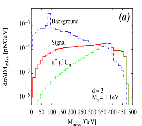
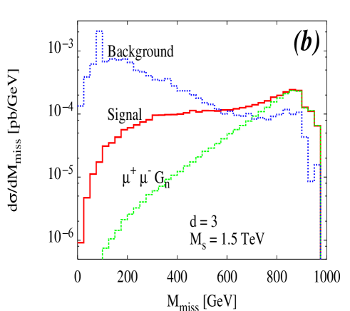
Figure 2: Distribution in missing invariant mass $M_{\rm miss}$ for $\sqrt{s}=$ ($a$) 500 GeV and ($b$) 1 TeV. In addition to total signal and background cross-sections, we also show the signal due to $s$-channel diagrams only, which is identical with the cross-section for $e^{+}e^{-}\to\mu+\mu^{-}G_{n}$.

Incorporating all these cuts into a Monte Carlo event generator, we obtain the distribution in missing invariant mass shown in Figure 2. It is clear from the figure that the missing invariant mass of the signal is much harder than that of the background. This is easy to understand if we realize that the missing mass is a measure of the energy of the emitted graviton. Now it is well-known that the higher the energy, the more strongly the graviton is coupled to matter and consequently the higher the production cross-section. Moreover, a higher energy leads to a higher density of states, and this further enhances the cross-section. In Figure 2, we have also shown the value of the signal when only $s$-channel diagrams are considered, which would be the case if we were to study processes like $e^{+}e^{-}\to\mu^{+}\mu^{-}G_{n}$ or $e^{+}e^{-}\to\tau^{+}\tau^{-}G_{n}$. Comparison with the signal of interest makes it obvious that there is a substantial contribution to the Bhabha scattering signal from the $t$-channel, which makes it more viable as a signal of ADD gravity than the other two. In fact, the emission of a high-energy graviton (corresponding to large missing invariant mass) reduces the energy of the underlying Bhabha scattering process, causing a large enhancement due to the $Z$-pole. This is the reason why the signal for large $M_{\rm miss}$ is completely dominated by the $s$-channel contribution. At the same time, when the graviton is relatively soft, the $s$-channel diagrams are strongly suppressed, but the $t$-channel contributions are not; as a result the signal is dominated by the $t$-channel contribution for low $M_{\rm miss}$. We can therefore obtain a clear separation of signal from background by imposing a cut

$$M_{\rm miss}>350~{}(450)~{}{\rm GeV~{}~{}for}~{}\sqrt{s}=500~{}{\rm GeV}~{}(1~{}{\rm TeV})$$

These choices are optimal, after taking into account the fact that the signal falls rapidly with increasing $M_{s}$ and $d$.

An important strategy for background reduction is the use of the beam polarization facility at a linear collider. If the electron (positron) beam has a right (left) polarization efficiency ${\cal P}_{e}$ (${\cal P}_{p}$), the cross-section formula corresponding to equation 2 is obtained by the replacement

$$\sum_{\lambda_{1},\lambda_{2}}|M_{n}(\lambda_{1},\lambda_{2})|^{2} \longrightarrow ~{}~{}~{}(1+{\cal P}_{e})(1-{\cal P}_{p})|M_{n}(+,+)|^{2}+(1+{\cal P}_{e})(1+{\cal P}_{p})|M_{n}(+,-)|^{2}$$

$$+~{}(1-{\cal P}_{e})(1-{\cal P}_{p})|M_{n}(-,+)|^{2}+(1-{\cal P}_{e})(1+{\cal P}_{p})|M_{n}(-,-)|^{2}$$

Typical values for the polarization efficiencies[1] used in this analysis are ${\cal P}_{e}=0.8$ and ${\cal P}_{p}=0.6$, which tend to favor the first two terms on the right side of the above expression. The use of polarized beams leads to a drastic reduction in the SM background, chiefly because it causes suppression of the $W$-induced diagrams. The numerical effects are presented in the next section.

4 Results and Discussions

After numerical evaluation of signal and background, we find it convenient to present our results, using the significance $S/\sqrt{B}$, where $S(B)={\cal L}\sigma_{S(B)}$, for given values of $d$ and $M_{S}$, Here $\sigma_{S(B)}$ denotes the cross-section for the signal (background), while ${\cal L}$ is the integrated luminosity. Our numerical results are presented assuming ${\cal L}=500$ fb^-1; however, it is a simple matter to scale the significance values for different values of luminosity.

In Figure 3($a$) we show curves showing the variation of the significance with the string scale $M_{S}$, for $d=2,3,4,5$ and $6$ respectively, for $\sqrt{s}=500$ GeV. Figure 3($b$) shows a similar plot for $\sqrt{s}=1$ TeV. In both cases, we have considered unpolarized electron and positron beams.

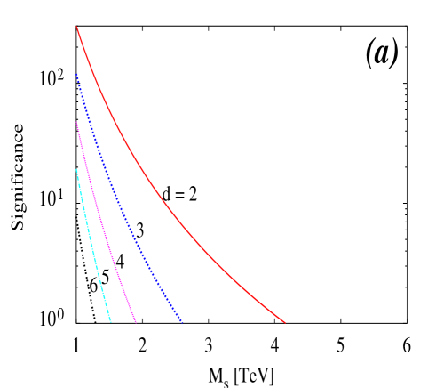
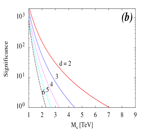
Figure 3: Illustrating the variation of significance $S/\sqrt{B}$ with $M_{S}$, considering unpolarized beams for ($a$) $\sqrt{s}=500$ GeV, and ($b$) $\sqrt{s}=1$ TeV.

As has been already mentioned, the use of beam polarization improves changes of detecting the signal quite dramatically. This is illustrated in Figure 4, which is similar to Figure 3, except that the polarization efficiencies have been taken to be ${\cal P}_{e}=0.8$ and ${\cal P}_{p}=0.6$ for the electron and positron respectively.

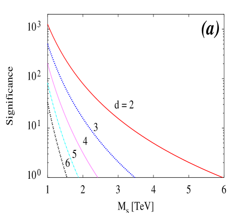
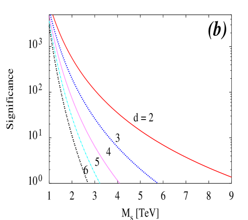
Figure 4: Illustrating the variation of significance $S/\sqrt{B}$ with $M_{S}$, considering polarized beams for ($a$) $\sqrt{s}=500$ GeV, and ($b$) $\sqrt{s}=1$ TeV. We take ${\cal P}_{e}=0.8$ and ${\cal P}_{p}=0.6$.

From the above graphs, it is straightforward to find out the maximum value of $M_{s}$ that can be probed at the linear collider for any given value of $d$, both for polarized and unpolarized beams. In Table 1, we present the values of $M_{s}$ that one can probe at 99% confidence level.

$$\begin{array}[]{|c|r|c|c|c|c|c|c|}\hline\cr\sqrt{s}&d=&2&3&4&5&6\\ \hline\cr\hline\cr 0.5&{\rm polarized}&4.53&2.79&2.01&1.60&1.35\\ &{\rm unpolarized}&3.16&2.09&1.59&1.30&1.12\\ \hline\cr\hline\cr 1.0&{\rm polarized}&7.40&4.63&3.41&2.76&2.36\\ &{\rm unpolarized}&5.36&3.57&2.74&2.28&2.36\\ \hline\cr\end{array}$$

Table 1. 99% C.L. discovery limits on the string scale $M_{S}$ for an ADD scenario using (graviton) radiative Bhabha scattering, for different numbers of extra dimensions. An integrated luminosity of $500~{}fb^{-1}$ has been assumed. All numbers are in TeV.

If one compares these with the corresponding reach of the process[4, 9, 10] $e^{+}e^{-}\to\gamma+\not{\!\!E}$, one will notice that search limits are approximately of the same order. However, the comparison should not be made too literally, because of several reasons. First, the polarization efficiencies in our case, while matching with those of [10], are different from those of [4], while the center-of-mass energy at which reference [10] has calculated the effects is slightly different from ours. In addition, one needs to match the event selection criteria more carefully for a full-fledged comparison. Finally, it should be borne in mind that in our analysis we have adopted a normalization of the string scale $M_{s}$, which, though widely used, is not necessarily uniform in the literature. However, in spite of such non-uniformities, Figures 3 and 4, together with Table 1, can perhaps be taken as faithful indications of the fact that the predictions on radiative Bhabha scattering are comparable to those on the photon-graviton channel, so far as the limits of the probe on the string scale in ADD models are concerned.

5 Pinning Down the Model

A few comments are in order on how to distinguish graviton signals involving missing energy from similar ones arising from other kinds of new physics. For example, let us consider the well-known process $e^{+}e^{-}\to\gamma G_{n}$, leading to a single-photon-plus-missing-energy signal. Such signals can be obtained in several other models. A model with an extra $Z^{\prime}$ boson could lead to a process $e^{+}e^{-}\to\gamma Z^{\prime}$ with the $Z^{\prime}$ decaying to neutrinos. Similarly, in supersymmetric models, a process like $e^{+}e^{-}\to\gamma\widetilde{\chi}^{0}_{1}\widetilde{\chi}^{0}_{1}$ (where $\widetilde{\chi}^{0}_{1}$ is the lightest neutralino) would also lead to a single photon signal. Although the $Z^{\prime}$ signal can be differentiated by looking for a resonant peak in the missing invariant mass, the supersymmetric signal is more difficult to disentangle.

The situation for the process considered in this paper is somewhat more encouraging. It is true that both types of new physics considered in the preceding paragraph can produce the same signal. Processes of the form $e^{+}e^{-}\to e^{+}e^{-}Z^{\prime}$, with the $Z^{\prime}$ decaying to neutrinos are one possibility. In supersymmetry, too, it is possible to pair-produce either sleptons or charginos, followed by decays to electrons (positrons) and invisible particles. The $Z^{\prime}$ signal can again be differentiated by a peak in the missing invariant mass. The supersymmetric signal, in this case, always arises from production of a pair of real sparticles, which should emerge in opposite hemispheres and, if light enough, will be highly boosted. As a result, the observed electron and positron should lie, most of the time, in opposite hemispheres. For the graviton signal, however, there is no such correlation; in fact the distribution in the opening angle between $e^{+}$ and $e^{-}$ turns out to be practically flat. This distinction clearly does not work very well when the produced sparticles are heavy.

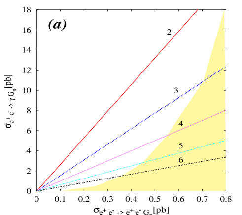
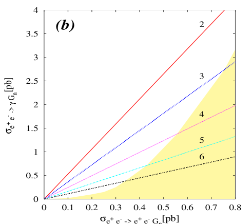
Figure 5: Correlation plot showing the polarized cross-sections for the processes $e^{+}e^{-}\to\gamma G_{n}$ and $e^{+}e^{-}\to e^{+}e^{-}G_{n}$ for different values of $d$. Each curve is generated by varying $M_{S}$ for ($a$) $\sqrt{s}=500$ GeV, and ($b$) $\sqrt{s}=1$ TeV. Shading indicates the region where the theoretical calculation is unreliable.

A more elegant way of distinguishing these signals from those other forms of new physics is to compare the cross-sections arising from both the processes $e^{+}e^{-}\to\gamma G_{n}$ and $e^{+}e^{-}\to e^{+}e^{-}G_{n}$, both of which are determined by the two parameters $d$ and $M_{S}$, and hence, will have some correlation. In Figure 5, we have plotted the cross-sections $\sigma(\gamma G_{n})$ versus $\sigma(e^{+}e^{-}G_{n})$ for different values of $d$. In view of the discussion in the previous section, we would like to note that here the rates for $e^{+}e^{-}\to\gamma G_{n}$ have been computed with the same normalization of the string scale as that used for the Bhabha scattering process. Each curve corresponds to variation of $M_{S}$ over the range allowed by current experimental constraints. Once experimental data are available from a high energy $e^{+}e^{-}$ machine, we should be able to pinpoint a small region (ideally a point) on the graph(s) in Figure 5. The position of this would immediately direct us to the value of $d$; comparison of the cross-sections would now yield a measurement of the value of $M_{S}$. The identification of the model parameters should be unambiguous since the curves for different values of $d$ do not intersect except at the origin. In any case, the area in the vicinity of the origin is limited by the search limits indicated in Table 1 since it corresponds to very high values of $M_{S}$. The shaded region corresponds to $M_{S}=\sqrt{s}$ beyond which the theoretical calculations are unreliable. It should, of course be remembered that further information on the fundamental parameters of theory can be extracted from various kinematic distributions which are sensitive to these parameters.

6 Summary and Conclusions

In the paper we have considered the process $e^{+}e^{-}\to e^{+}e^{-}G_{n}$, which is essentially Bhabha scattering with radiated gravitons in the ADD model. After identifying suitable event selection criteria, we find that this process can act as an effective probe of large extra dimensions at a high-energy $e^{+}e^{-}$ collider, especially with a center-of-mass energy of order 1 TeV and with polarized beams. The string scale $M_{S}$ that can be probed in this channel is found to be comparable to that which is accessible through the alternative process $e^{+}e^{-}\to\gamma G_{n}$. It is also shown that a study of the (graviton) radiative Bhabha scattering process may provide some further handle on the essential characteristics of ADD-like theories. And finally, taking a cue from the wisdom that, in coming to any conclusion on new physics possibilities, it is always advantageous to have more than one type of data, we have demonstrated how our predictions can be combined with those on the photon-graviton channel to obtain rather trustworthy revelations on models with large extra dimensions.

Acknowledgments

The authors acknowledge useful discussions with D.Choudhury, R.M.Godbole, U.Mahanta, and S.K.Rai. This work was initiated as part of the activity of the Indian Linear Collider Working Group (Project No. SP/S2/K-01/2000-II of the Department of Science and Technology, Government of India). SD thanks the SERC, Department of Science and Technology, Government of India for partial support. The work of BM was partially supported by the Board of Research in Nuclear Sciences (BRNS), Government of India. SR thanks the Harish-Chandra Research Institute for hospitality while this paper was being written.

References

- [1] ECFA/DESY LC Physics Working Group Report, J.A. Aguilar-Savedra et al, hep-ph/0106315 (2001); Snowmass Report, S. Kuhlman et al, hep-ex/9605011 (1996).
- [2] K. Akama, Lect. Notes Phys. 176, 267 (1982); V. Rubakov and M. Shaposhnikov, Phys. Lett. B125, 136 (1983) ; ibid. 125, 139, (1983); A. Barnaveli and O. Kancheli, Sov. J. Nucl. Phys. 51, 573 (1990); I. Antoniadis, Phys. Lett. B246, 377 (1990) ; I. Antoniadis, C. Muñoz and M. Quiros, Nucl. Phys. B397, 515 (1993) ; I. Antoniadis, K. Benakli and M. Quiros, Phys. Lett. B331, 313 (1994) .
- [3] N. Arkani-Hamed, S. Dimopoulos and G. Dvali, Phys. Lett. B429, 263 (1998) ; I. Antoniadis, N. Arkani-Hamed, S. Dimopoulos and G. Dvali, Phys. Lett. B436, 257 (1998) ; N. Arkani-Hamed, S. Dimopoulos and G. Dvali, Phys. Rev. D59, 086004 (1999) .
- [4] G.F. Giudice, R. Rattazzi and J.D. Wells, Nucl. Phys. B544, 3 (1998) .
- [5] T. Han, J.D. Lykken and R.-J. Zhang, Phys. Rev. D59, 105006 (1999) .
- [6] J.C. Long et al, Nature, 421, 922 (2003).
- [7] See, for example, J. Polchinski, Tasi Lectures on D-Branes, hep-th/9611050 (1996).
- [8] For a very readable review, see, for example, Y.A. Kubyshin, hep-ph/0111027 (2001).
- [9] E.A. Mirabelli, M. Perelstein and M.E. Peskin, Phys. Rev. Lett. 82, 2236 (1999) ; S. Cullen, M. Perelstein and M. Peskin, Phys. Rev. D62, 055012 (2000) .
- [10] G.W. Wilson, in 2nd ECFA/DESY Study 1998-2001, p.1506 (2001).
- [11] O.J.P. Eboli et al, Phys. Rev. D64, 035005 (2001) .
- [12] H. Murayama, I. Watanabe and K. Hagiwara, KEK preprint KEK-91-11 (1992).
- [13] C.H. Chen, M. Drees and J.F. Gunion, Phys. Rev. Lett. 76, 2002 (1996) ; Erratum-ibid. 82, 3192 (1999).
- [14] W. Kozanecki et al, Saclay preprint DAPNIA-SPP-92-04 (1992).