Nonlinear dynamics of soft boson
collective excitations in hot QCD plasma II:
plasmon – hard-particle scattering and energy losses

$${\bf Abstract}$$

In a general line with our first work [1], within hard thermal loop (HTL) approximation a general theory of the scattering for an arbitrary number of colorless plasmons off hard thermal particles of hot QCD-medium is considered. Using generalized Tsytovich correspondence principle, a connection between matrix elements of the scattering processes and a certain effective current, generating these processes is established. The iterative procedure of calculation of these matrix elements is defined, and a problem of their gauge-invariance is discussed. An application of developed theory to a problem of calculating energy losses of energetic color particle propagating through QCD-medium is considered. It is shown that for limiting value of the plasmon occupation number ($\sim 1/g^{2}$, where $g$ is a strong coupling) energy losses caused by spontaneous scattering process of energetic particle off soft-gluon waves is of the same order in the coupling as other known losses type: collision and radiation ones. The Fokker-Planck equation, describing decceleration (acceleration) and diffusion in momentum space of beam of energetic color particles scattering off soft excitations of quark-gluon plasma (QGP), is derived.

1 Introduction

In the second part of our work we carry on with analysis of dynamics of boson excitations in hot QCD-medium at the soft momentum scale, started in [1] (to be reffered to as “Paper I” throughout this text) in the framework of HTL effective theory [2]. Here, we focuss our research on the studies of the scattering processes of soft-gluon plasma waves off hard particles of higher order within a real time formalism based on a Boltzmann type kinetic equation for soft modes. The nonlinear Landau damping process studied before [3] is simple example of this type of scattering processes. In a similar case of plasmon-plasmon scattering [1], for sufficiently high energy level of the soft plasma excitations (exact estimation will be given in Section 5 below) all higher processes of plasmon – hard-partical scattering will give a contribution of the same order to the right-hand side of the Boltzmann equation.

Our approach is based on the system of dynamical equations derived by Blaizot and Iancu [4] complemented by famous Wong equation [5] that describes the precession of the classical color charge $Q=(Q^{a}),\,a=1,\ldots,N_{c}^{2}-1$ for hard particle in a field of incident soft-gluon plasma wave. Using the so-called Tsytovich correspondence principle introduced in Paper I with necessary minimal generalization for relevant problem, we establish a link between matrix elements of studied scattering processes and a certain effective currents, generating these processes. These effective currents appear in solving combined equation system of Blaizot-Iancu and Wong’s equations in the form of expansion in powers of free gauge field $A_{\mu}^{(0)a}$ and initial value of a color charge $Q_{0}^{a}$. The coefficient functions in this expansion determines matrix elements of investigated scattering processes. The appearance of classical soft-gluon loop corrections to the scattering processes, that in leading order in coupling can be formally presented in the form of tree diagramm with vertices and propagators in HTL or eikonal approximations, here, is a new interest ingredient.

We apply the current approach to study of the propagation of high energy color parton (gluon or quark) through a hot QCD-medium and energy losses associated with this motion. Research of the energy losses of energetic partons in QGP at present is of a great interest with respect to jet quenching phenomenon [6, 7, 8, 9] and its related high-$p_{t}$ azimuthal asymmetry [10, 11], large-$p_{t}$ $\pi^{0}$ suppression [12, 13] etc., that have observed in ultrarelativistic heavy ion collisions at RHIC (see, review [14]). Throughout the past twenty years by the efforts of many authors several possible mechanisms of energy losses have been analyzed: (1)elastic small distance collisional losses due to the final state interaction of high energy parton with medium constituent (Bjorken [15], Braaten and Thoma [16]); (2)polarization losses or losses caused by large distance collision (Thoma and Gyulassy, Mrówczyński, Koike and Matsui [17], Braaten and Thoma [16]); (3)losses due to gluon bremsstrahlung induced by multiple scattering (Ryskin [18]; Gyulassy, Wang and Plümmer [19], Baier at al. [20, 21, 22], Zakharov [23], Levin [24], Wiedemann [25], Kovner and Wiedemann [26] etc.). The first two mechanisms often combined into one collision mechanism of energy loss, but it is convenient for our purpose to separated them.

It was shown [6] that the elastic and polarization energy losses of partons in QCD plasma turned out to be too small for jet extinction, while induced radiative energy losses prove to be sufficient large to make itself evident in jet quenching in collisions of heavy nuclei. For this reason recent theoretical stydies of parton energy loss have concentrated on gluon radiation [19] – [26].

However these ‘traditional’ approaches have difficulties accounting for the large jet losses reported at RHIC [14]. This is the motivation for more detail analysis of mechanisms of energy losses already studied or their alternative formulations (in particulary, radiation losses) as well as the considered novel mechanisms. To the first case it can be assigned the works of Gyulassy, Levai and Vitev on construction an algebraic reaction operator formalism [28], twist expansion approach developed by Wang et al. [29]. The work of Shuryak and Zahed [30] considered synchrotron-like radiation in QCD by generalized Schwinger’s treatment of quantum synchrotron radiation in QED, a work of E. Wang and X.-N. Wang [31] connected with allowing for stimulated gluon emission and thermal absorption by the propagating parton in dense QGP, and also mechanism of coherent final state interaction proposed by Zakharov [32], can be assigned to the second case.

In this work we would like to turn to study of just one more mechanism of loss (or gain) energy, the special and simplest case of which is polarisation loss. The approximation within of which polarization loss is calculated, valids only for extremely low level of excitations for soft fields of medium. This is circumstance on which it was indicated by Mrówczyński in Ref. [17]. The expression for polarization part of energy loss derived in [17] up to color factors is exactly coincident with expression obtained early in the theory of usual plasma [33] within standard linear response theory. However, we can expect that for ultrarelativistic heavy ion collisions generated QGP will be far from equilibrium in highly excited state. It can be valid at least for the subsystem of soft plasmons (Section 2, Paper I), when interaction by soft waves preponderate over effects of particle collisions. One could study the influence of such off-equilibrium effects on parton propagation and radiation for unbounded QGP. For existence of intensity of soft radiation in medium, additional mechanism of deceleration (or acceleration) of energetic color particle connected with spontaneous and stimulated scattering processes of this particle off soft gluon excitations arises. In a limiting case of a strong gauge field $|A_{\mu}^{a}(X)|\sim T$, where $T$ is a temperature of a system, this type of energy losses becomes of the same order in $g$ as above mechanisms of energy losses and therefore can give quite appreciable contribution to total losses balance (this problem is discussed in more detail in Section 7 and 8 of present work). It is precisely here non-Abelian character of interaction of hard color particle with soft-gluon field in QGP is to be completely manifested. The first work, where an attempt was made to accounting for interaction of energetic (massive) colored particle with stochastic background chromoelectric field, using the semiclassical equations of motion, is the work of Leonidov [34]. In this work an approach developed to the problem of stochastic deceleration and acceleration of cosmic rays in usual plasma [35] has been used. However here, no account has been taken the fact that in the case of dense medium, what is QGP, in the scattering process, plasma surrounding traveling color charge not remains indifferent towards. In QGP the nonlinear polarization currents arise, essentially varying a physical picture. In the case of Abelian plasma this was shown by Gailitis and Tsytovich in [36]. To account for polarization currents it is necessary to use a kinetic equation, that were not made in above-mentioned work by Leonidov.

A more close to the subject of our research on a conceptional plane is the work of E. Wang and X.-N. Wang [31] have been already cited above. Here, at the first a problem of influence on energy losses of stimulated gluon emission and thermal absorption by the propagating parton because of the presence of hard thermal gluons in the hot QCD-medium, was posed. This mechanism of energy losses is important in a medium with large initial gluon density (such it is proportional to gluon density) that it is really possible takes place by virtue of a strong suppression of high transverse momentum hadron spectra observed by experiments at RHIC [14]. However, in Ref [31] only gluon emission and absorption of hard thermal gluons (whose energy is of order $T$) with the use of the methods of perturbative QCD, is considered. For large density of soft gluon radiation consideration of contribution to energy loss of soft emission and absorption by the propagating parton, also becomes important. These processes (proportional to soft-gluon number density) by virtue of large occupation number of soft excitations adequately describe by using quasiclassical methods based on HTL approaches.

Returning to the problem stated in this work, it is necessary run ahead note the following important circumstance: effective currents, determining the processes of spontaneous and stimulated scattering posses remarkable pecularity that they not explicitly dependent on mass of hard particle (in HTL-approximation), and therefore developed theory is suitable equally for light color particle as well as massive ones. This in particular is reflected in that losses caused for instance by spontaneous scattering of energetic particle off soft excitations will be connected with not varying momentum of particle, but with rotation of its (classical) color charge in effective color space, governing by Wong equation. Here, we have a principal distinction from energy loss of charge particles in usual plasma. In Abelian case as known [33], a rate of energy loss (or gain) for interaction with stochastic plasma field is inverse propotional to mass of hard particle, and therefore it is essential for light particles (electron, positron) and suppressed for heavy ones (proton, ion), although their polarization losses are practically identical. In non-Abelian plasma, at least within HTL-approximation the mass dependence can enter only through integration limits and a value of velocity of energetic parton, and therefore explicit suppression by mass of this energy loss type, is not arisen. In this connection note that study of propagation of heavy partons ($c$ or $b$ quarks) through QGP is of great independent interest. The first estimation of energy loss of heavy quark will be made by Svetitsky [37] for study of the diffusion process of charmed quark in QGP, and then the estimation will be given also in the works by Braaten and Thoma [16] Mustafa et al., Walton and Rafelski [38](collision losses), and Mustafa et al. [39], Dokshitzer and Kharzeev [40](radiation losses). The energy losses of heavy quarks are important not only with jet quenching phenomenon, but also for other important one for diagnostic of QGP: the modification of the high mass dimuon spectra from semileptonic $B$ and $D$ meson decays (Shuryak, Lin, Vogt and Wang [41], Kämpfer et al., Lokhtin and Snigirev [42]).

Paper II is organized as follows. In Section 2 preliminary comments with regard to derivation of the Boltzmann equation taking into account the scattering processes of an arbitrary number of colorless plasmons off hard thermal particles, are given. Section 3 presents a detailed consideration of the kinetic equation for the nonlinear Landau damping process, and here, also appropriate extension of the Tsytovich correspondence principle is presented. In Section 4 a complete algorithm of the succesive calculation of the certain effective currents, generating considered scattering processes, is given. In Section 5 on the based of the correspondence principle these effective currents are used for calculation of the proper matrix elements. Here, we estimate the typical value of plasmon occupation numbers, wherein one can restricted the consideration to acounting for only the contribution from the nonlinear Landau damping process or all higher scattering processes should be considered. In Section 6 we discuss a problem of a gauge independence of matrix elements defined in previous Section. Section 7 is concerned with definition of general quasiclassical expressions for energy loss of energetic color particle for its scattering off soft plasma excitations. In Section 8 the energy loss caused by spontaneous scattering off colorless plasmons in lower order in powers of plasmon number density is analyzed in detail, and in Section 9 some problems connected with scattering of energetic particle by soft-gluon excitations lying off mass-shell, is discussed. Finally in Section 10 the Fokker-Planck equation, describing an evolution of a distribution function for a beam of energetic color partons scattering off plasmons, is derived. In the closing section we briefly discuss some interest and important moments concerned with mechanism of energy loss studied in this work, and remaining to be considered.

2 Preliminares

As in Paper I we consider a pure gluon plasma with no quarks, where soft longitudinal excitations is propagated. Here, we restrict our cosideration to soft colorless exsitations, i.e. we assume that a localized number density of plasmons $N^{l}({\bf p},x)\equiv(N_{\bf p}^{l\,ab})$ is diagonal in color space

$$N_{\bf p}^{l\,ab}=\delta^{ab}N_{\bf p}^{l},$$

where $a,b=1,\ldots,N_{c}^{2}-1$ for $SU(N_{c})$ gauge group. We consider in Paper II the change of the number density of the colorless plasmons $N_{\bf p}^{l}$ as result of their scattering off hard thermal gluons. We expect in this case that the time-space evolution of scalar function $N_{\bf p}^{l}$ will be described by

$$\frac{\partial N_{\bf p}^{l}}{\partial t}+{\bf v}_{\bf p}^{l}\cdot\frac{\partial N_{\bf p}^{l}}{\partial{\bf x}}=-N_{\bf p}^{l}\Gamma_{\rm d}[N_{\bf p}^{l}]+(1+N_{\bf p}^{l})\Gamma_{\rm i}[N_{\bf p}^{l}]\equiv-C[N_{\bf p}^{l}],$$ (2.1)

where ${\bf v}_{\bf p}^{l}=\partial\omega_{\bf p}^{l}/\partial{\bf p}$ is a group velocity of the longitudinal oscillations and $\omega_{\bf p}^{l}\equiv\omega^{l}({\bf p})$ is the dispersion relation for plasmons. As it usually is, a functional dependence is denoted by argument of a function in square brackets.

The more general expressions for generalized decay rate $\Gamma_{\rm d}$ and regenerating rate $\Gamma_{\rm i}$ can be written in the form of functional expansion in powers of the plasmon number density

$$\Gamma_{\rm d}[N_{\bf p}^{l}]=\sum_{n=0}^{\infty}\Gamma_{\rm d}^{(2n+1)}[N_{\bf p}^{l}],\;\;\Gamma_{\rm i}[N_{\bf p}^{l}]=\sum_{n=0}^{\infty}\Gamma_{\rm i}^{(2n+1)}[N_{\bf p}^{l}],$$ (2.2)

where

$$\Gamma_{\rm d}^{(2n+1)}[N_{\bf p}^{l}]=\int\!\frac{d{\bf k}}{(2\pi)^{3}}\!\int\!{\rm d}{\cal T}^{(2n+1)}\,{\it w}_{2n+2}({\bf k}|\,{\bf p},{\bf p}_{1},\ldots,{\bf p}_{n};{\bf p}_{n+1},\ldots,{\bf p}_{2n+1})$$ (2.3)

$$\times N_{{\bf p}_{1}}^{l}\ldots N_{{\bf p}_{n}}^{l}(1+N_{{\bf p}_{n+1}}^{l})\ldots(1+N_{{\bf p}_{2n+1}}^{l})f_{\bf k}[1+f_{{\bf k}^{\prime}}],$$

$$\Gamma_{\rm i}^{(2n+1)}[N_{\bf p}^{l}]=\int\!\frac{d{\bf k}}{(2\pi)^{3}}\!\int\!{\rm d}{\cal T}^{(2n+1)}\,{\it w}_{2n+2}({\bf k}|\,{\bf p},{\bf p}_{1},\ldots,{\bf p}_{n};{\bf p}_{n+1},\ldots,{\bf p}_{2n+1})$$ (2.4)

$$\times(1+N_{{\bf p}_{1}}^{l})\ldots(1+N_{{\bf p}_{n}}^{l})N_{{\bf p}_{n+1}}^{l}\ldots N_{{\bf p}_{2n+1}}^{l}f_{{\bf k}^{\prime}}[1+f_{\bf k}].$$

Here, $f_{\bf k}\equiv f({\bf k},x)$ is the disribution function of hard thermal gluons, and the phase-space integration is

$$\int\!{\rm d}{\cal T}^{(2n+1)}\!\equiv\!\int(2\pi)\delta(E_{\bf k}+{\cal E}_{\rm in}-E_{{\bf k}+{\bf p}_{\rm in}-{\bf p}_{\rm out}}-{\cal E}_{\rm out})\!\prod_{i=1}^{2n+1}\!\frac{d{\bf p}_{i}}{(2\pi)^{3}},$$ (2.5)

where

$${\cal E}_{\rm in}=\omega^{l}_{\bf p}+\omega^{l}_{{\bf p}_{1}}+\ldots+\omega^{l}_{{\bf p}_{n}},\quad{\bf p}_{\rm in}={\bf p}+{\bf p}_{1}+\ldots+{\bf p}_{n},\hskip 8.5359pt$$

$${\cal E}_{\rm out}=\omega^{l}_{{\bf p}_{n+1}}+\ldots+\omega^{l}_{{\bf p}_{2n+1}},\quad{\bf p}_{\rm out}={\bf p}_{n+1}+\ldots+{\bf p}_{2n+1},$$

are total energies and momenta of incoming and outgoing external plasmon legs, respectively, and $E_{\bf k}=|{\bf k}|$ for massless hard gluons.

The $\delta$-function in Eq. (2.5) expresses the energy conservation of the processes of stimulated emission and absorption of the plasmons. The function

$${\it w}_{2n+2}={\it w}_{2n+2}({\bf k}|\,{\bf p},{\bf p}_{1},\ldots,{\bf p}_{n};{\bf p}_{n+1},\ldots,{\bf p}_{2n+1})$$ (2.6)

is a probability of absorption of $n+1$ plasmons with frequencies $\omega_{\bf p}^{l},\,\omega_{{\bf p}_{1}}^{l},\ldots,\omega_{{\bf p}_{n}}^{l}$ (and appropriate wavevectors ${\bf p},\,{\bf p}_{1},\ldots,{\bf p}_{n}$) by a hard thermal gluon carrying momentum ${\bf k}$ with consequent radiation of $n+1$ plasmons with frequencies $\omega_{{\bf p}_{n+1}},\ldots\omega_{{\bf p}_{2n+1}}$ (and the wavevectors ${\bf p}_{n+1},\ldots,{\bf p}_{2n+1}$). We note that for generalized decay and regenerated rates (2.3) and (2.4) it was assumed that the scattering probability (2.6) satisfies the symmetry relation over permutation of incoming and outgoing soft plasmon momenta

$${\it w}_{2n+2}({\bf k}|\,{\bf p},{\bf p}_{1},\ldots,{\bf p}_{n};{\bf p}_{n+1},\ldots,{\bf p}_{2n+1})={\it w}_{2n+2}({\bf k}|\,{\bf p}_{n+1},\ldots,{\bf p}_{2n+1};{\bf p},{\bf p}_{1},\ldots,{\bf p}_{n}).$$ (2.7)

This relation is a consequence of more general relation for exact scattering probability depending on initial and final values of momentum of hard particle, namely,

$${\it w}_{2n+2}({\bf k},{\bf k}^{\prime}|\,{\bf p},{\bf p}_{1},\ldots,{\bf p}_{n};{\bf p}_{n+1},\ldots,{\bf p}_{2n+1})={\it w}_{2n+2}({\bf k}^{\prime},{\bf k}|\,{\bf p}_{n+1},\ldots,{\bf p}_{2n+1};{\bf p},{\bf p}_{1},\ldots,{\bf p}_{n}).$$

It expresses detailed balancing principle in scattering processes, and in this sence it is exact. The scattering probability (2.6) is obtained by integrating of total probability over ${\bf k}^{\prime}$ with regard to momentum conservation law:

$${\it w}_{2n+2}({\bf k}|\,{\bf p},{\bf p}_{1},\ldots,{\bf p}_{n};{\bf p}_{n+1},\ldots,{\bf p}_{2n+1})\,2\pi\delta(E_{\bf k}+{\cal E}_{\rm in}-E_{{\bf k}+{\bf p}_{\rm in}-{\bf p}_{\rm out}}-{\cal E}_{\rm out})$$

$$=\int\!{\it w}_{2n+2}({\bf k},{\bf k}^{\prime}|\,{\bf p},{\bf p}_{1},\ldots,{\bf p}_{n};{\bf p}_{n+1},\ldots,{\bf p}_{2n+1})\,2\pi\delta(E_{\bf k}+{\cal E}_{\rm in}-E_{{\bf k}^{\prime}}-{\cal E}_{\rm out})$$

$$\times\,(2\pi)^{3}\delta({\bf k}+{\bf p}_{\rm in}-{\bf k}^{\prime}-{\bf p}_{\rm out})\,\frac{d{\bf k}^{\prime}}{(2\pi)^{3}}.$$

Such obtained scattering probability satisfies the relation (2.7) in a limit of interest to us, i.e. when we neglect by (quantum) recoil of test particle. In the general case the expression (2.7) is replaced by more complicated one (see Section 10).

In Eqs. (2.3) and (2.4) as in the case of pure plasmon-plasmon interaction (Paper I), we take into account the scattering processes only with equal number of the plasmons prior to interaction and upon it, i.e. the scattering processes of the following ”elastic“ type

$${\rm g}^{\ast}+{\rm G}\rightleftharpoons{\rm g}_{1}^{\ast}+{\rm G}^{\prime},\quad{\rm for}\;n=0,$$

$${\rm g}^{\ast}+{\rm g}_{1}^{\ast}+{\rm G}\rightleftharpoons{\rm g}_{2}^{\ast}+{\rm g}_{3}^{\ast}+{\rm G}^{\prime},\quad{\rm for}\;n=1,$$ (2.8)

$$\ldots,$$

where ${\rm g}^{\ast},\,{\rm g}_{1}^{\ast},\ldots$ are plasmon collective excitations and ${\rm G},\,{\rm G}^{\prime}$ are excitations with characteristic momenta of order $T$. The scattering processes with odd number of the plasmons are kinematically forbidden by the conservation laws. Finally the scattering processes with unequal even number of incoming and outgoing soft external legs, i.e. the processes of “inelastic” type

$${\rm G}\rightleftharpoons{\rm g}^{\ast}+{\rm g}_{1}^{\ast}+{\rm G}^{\prime},\quad{\rm for}\;n=0,$$

$${\rm g}^{\ast}+{\rm g}_{1}^{\ast}+{\rm G}\rightleftharpoons{\rm g}_{2}^{\ast}+{\rm g}_{3}^{\ast}+{\rm g}_{4}^{\ast}+{\rm g}_{5}^{\ast}+{\rm G}^{\prime},\quad{\rm for}\;n=2,$$

etc., have kinematic regions of momentum variables accessible by conservation laws not coincident with kinematic regions of the corresponding processes of elastic type (2.8), and we suppose that a contribution of the last processes to the nonlinear plasmon dynamics of the order of our interest is not important.

The scattering process for $n=0$ (Eq. (2.8)) known as the process of nonlinear Landau damping [33], in the case of a quark-gluon plasma was studied in detail in Ref. [3] (we will consider this process in the following section in the somewhat different context). In the present work we would like to extend the approach developed in [3] to the scattering processes involving arbitrary number of plasmons.

By using the fact that $|{\bf k}|\gg|{\bf p}|,\,|{\bf p}_{1}|,\ldots,|{\bf p}_{2n+1}|$, the energy conservation law can be represented in the form of the following “generalized” resonance condition

$${\cal E}_{\rm in}-{\cal E}_{\rm out}-{\bf v}\cdot({\bf p}_{\rm in}-{\bf p}_{\rm out})=0,\quad{\bf v}={\bf k}/|{\bf k}|.$$ (2.9)

In particular for $n=0$ we have resonance condition

$$\omega_{\bf p}^{l}-\omega_{{\bf p}_{1}}^{l}-{\bf v}\cdot({\bf p}-{\bf p}_{1})=0,$$ (2.10)

defining the nonlinear Landau damping process. Furthermore, one can approximate the distribution function of hard thermal gluons on the right-hand side of Eqs. (2.3) and (2.4)

$$f_{{\bf k}^{\prime}}\simeq f_{\bf k}+({\bf p}_{\rm in}-{\bf p}_{\rm out})\cdot\frac{\partial f_{\bf k}}{\partial{\bf k}},$$ (2.11)

and set $1+f_{\bf k}\simeq 1+f_{{\bf k}^{\prime}}\simeq 1$ by virtue of $f_{\bf k},\;f_{{\bf k}^{\prime}}\ll 1$.

We introduce the following assumption. We suppose that characteristic time for nonlinear relaxation of the soft oscillations is a small quantity compared with the time of relaxation of the distribution of hard gluons $f_{\bf k}$. In other words the intensity of soft plasma excitations are sufficiently small and they cannot essentially change such ‘crude’ equilibrium parameters of plasma as particle density, temperature and thermal energy. Therefore, we neglect by a space-time change of the distribution function $f_{\bf k}$, assuming that this function is specified and describe the global equilibrium state of non-Abelian plasma

$$f_{\bf k}=2\,\frac{1}{{\rm e}^{E_{\bf k}/T}-1}.$$

Here, the coefficient 2 takes into account that the hard gluon has two helicity states. In the context of this assumption (as it will be further shown) the scattering probability ${\it w}_{2n+2}({\bf k}|\,{\bf p},{\bf p}_{1},\ldots{\bf p}_{2n+1})$ depends upon the velocity ${\bf v}$ (a unit vector), but not upon the magnitude $|{\bf k}|$ of the hard momentum. This enables us somewhat simplify expression for collision term $C[N_{\bf p}^{l}]$.

We use the fact that the occupation numbers $N^{l}_{{\bf p}_{i}}$ are more large than one, i.e. $1+N_{{\bf p}_{i}}^{l}\simeq N_{{\bf p}_{i}}^{l}$. Furthermore we present the integration measure as

$$\int\!\frac{d{\bf k}}{(2\pi)^{3}}=\int\!\frac{d|{\bf k}|}{2\pi^{2}}\,|{\bf k}|^{2}\!\int\!\frac{d\Omega_{\bf v}}{4\pi},$$

where the solid integral is over the directions of unit vector ${\bf v}$. Taking into account above-mentioned, considering (2.11), the collision term can be approximated by following expression

$$C[N_{\bf p}^{l}]\simeq\bigg{(}\int\!\frac{d|{\bf k}|}{2\pi^{2}}\,|{\bf k}|^{2}\frac{\partial f_{\bf k}}{\partial|{\bf k}|}\bigg{)}\sum_{n=0}^{\infty}\int\!\frac{d\Omega_{\bf v}}{4\pi}\int\!d{\cal T}^{(2n+1)}$$ (2.12)

$$\times({\cal E}_{\rm in}-{\cal E}_{\rm out}){\it w}_{2n+2}({\bf v}|\,{\bf p},{\bf p}_{1},\ldots,{\bf p}_{n};{\bf p}_{n+1},\ldots,{\bf p}_{2n+1})N_{\bf p}^{l}N_{{\bf p}_{1}}^{l}\ldots N_{{\bf p}_{2n+1}}^{l}.$$

To derive the scattering probability ${\it w}_{2n+2}$ in Section 5 we need somewhat different approximation of collision term. Setting $1+N_{{\bf p}_{i}}^{l}\simeq N_{{\bf p}_{i}}^{l}$ and $f_{{\bf k}^{\prime}}\simeq f_{\bf k}$, in the limit of a small intensity $N_{\bf p}^{l}\rightarrow 0$ we have the following expression for collision term

$$C[N_{\bf p}^{l}]|_{N_{\bf p}^{l}\rightarrow 0}\simeq\biggl{(}\int\!\frac{d|{\bf k}|}{2\pi^{2}}\,|{\bf k}|^{2}f_{\bf k}\biggr{)}\sum_{n=0}^{\infty}\int\!\frac{d\Omega_{\bf v}}{4\pi}\int\!d{\cal T}^{(2n+1)}$$ (2.13)

$$\times{\it w}_{2n+2}({\bf v}|\,{\bf p},{\bf p}_{1},\ldots,{\bf p}_{n};{\bf p}_{n+1},\ldots,{\bf p}_{2n+1})N_{{\bf p}_{1}}^{l}\ldots N_{{\bf p}_{2n+1}}^{l}.$$

The kinetic equation (2.1) with collision term in the form of (2.13) defines a change of plasmons number, caused by processes of spontaneous plasmon scattering off hard test gluon only.

3 Nonlinear Landau damping process

In this section, we review the main features of the scattering probability for nonlinear Landau damping process derived in Ref. [3]. This will be done by another way (that has already used in Paper I) using Tsytovich correspondence principle [36], [43], admitting a direct extension to calculation of scattering probabilities for the processes of a higher order. We preliminary discuss a basic equation for a soft gauge field, that will play a main role in our subsequent research. We have already written out this equation in Paper I (Eq. (I.3.8)). Here, it should be correspondingly extented to take into account the presence of a current caused by test particle passing through hot gluon plasma.

One expects the word lines of the hard modes to obey classical trajectories in the manner of Wong [5] since their coupling to the soft modes is weak at very high temperature. Considering this circumstance, we add the color current of color point charge

$$j_{Q}^{a\mu}(x)=gv^{\mu}Q^{a}{\delta}^{(3)}({\bf x}-{\bf v}t)$$ (3.1)

to the right-hand side of the basic field equation. Here, $Q^{a}$ is a color classical charge. Considering $Q^{a}$ as a constant quantity we lead to the nonlinear integral equation for gauge potential $A_{\mu}$ instead of Eq. (I.3.8)

$$\,{}^{\ast}\tilde{\cal D}^{-1\,\mu\nu}(p)A^{a}_{\nu}(p)=-J^{a\mu}_{NL}[A](p)-j_{Q}^{a\mu}(p),$$ (3.2)

where

$$J^{a\mu}_{NL}[A](p)=\sum_{s=2}^{\infty}J^{(s)a\mu}(A,\ldots,A),$$ (3.3)

$$J^{(s)a}_{\mu}(A,\ldots,A)=\frac{1}{s!}\,g^{s-1}\!\!\int\!\!\,^{\ast}\Gamma^{aa_{1}\ldots a_{s}}_{\mu\mu_{1}\ldots\mu_{s}}(p,-p_{1},\ldots,-p_{s})A^{a_{1}\mu_{1}}(p_{1})A^{a_{2}\mu_{2}}(p_{2})\ldots A^{a_{s}\mu_{s}}(p_{s})$$

$$\times{\delta}^{(4)}(p-\sum_{i=1}^{s}p_{i})\prod_{i=1}^{s}dp_{i},$$

and

$$j_{Q}^{a\mu}(p)=\frac{g}{(2\pi)^{3}}\,v^{\mu}Q^{a}\delta(v\cdot p).$$ (3.4)

Here, we recall that the coefficient functions $\,{}^{\ast}\Gamma^{aa_{1}\ldots a_{s}}_{\mu\mu_{1}\ldots\mu_{s}}$ are usual HTL-amplitudes and $\,{}^{\ast}\tilde{\cal D}^{\mu\nu}(p)$ is a medium modified (retarded) gluon propagator in a temporal gauge defined by Eqs. (I.3.10) – (I.3.12).

As in Paper I (Section 5) we consider a solution of the nonlinear integral equation (3.2) by the approximation scheme method. Discarding the nonlinear terms in $A_{\mu}^{a}$ on the right-hand side, we obtain in the first approximation

$$\,{}^{\ast}\tilde{\cal D}^{-1\,\mu\nu}(p)A_{\nu}^{a}(p)=-j_{Q}^{a\mu}(p).$$

The general solution of the last equation is

$$A_{\mu}^{a}(p)=A_{\mu}^{(0)a}(p)-\,^{\ast}\tilde{\cal D}_{\mu\nu}(p)j_{Q}^{a\nu}(p),$$ (3.5)

where $A_{\mu}^{(0)a}(p)$ is a solution of homogeneous equation (a free field), and the last term on the right-hand side represents a gauge field induced by test parton in medium.

Furthermore, we keep the term quadratic in field on the right-hand side of Eq. (3.2). Substituting derived solution (3.5) into the right-hand side, we obtain the following correction to the interacting field

$$A_{\mu}^{(1)a}(p)=-\!\,^{\ast}\tilde{\cal D}_{\mu\nu}(p)J^{(2)a\nu}(A^{(0)},A^{(0)})\,-\!\,^{\ast}\tilde{\cal D}_{\mu\nu}(p)\{J^{(2)a\nu}(A^{(0)},-\!\,^{\ast}\tilde{\cal D}j_{Q})+J^{(2)a\nu}(-\!\,^{\ast}\tilde{\cal D}j_{Q},A^{(0)})\}$$

$$-\!\,^{\ast}\tilde{\cal D}_{\mu\nu}(p)J^{(2)a\nu}(-\!\,^{\ast}\tilde{\cal D}j_{Q},-\!\,^{\ast}\tilde{\cal D}j_{Q})\}.$$

The last term on the right-hand side of this expression equals zero by virtue of $f^{abc}Q^{b}Q^{c}=0$. The first term is associated with a pure plasmon-plasmon interaction and was analyzed previously in Paper I. Therefore now we have concentrated on new nontrivial terms putting in braces. Using explicit definition of the nonlinear current of the second order (Eq. (3.3)) it can be shown that a second term in braces equals the first one.

We determine thus a new effective current (more exactly, the first term in the expansion over free field) that is a correction to “starting” current (3.4), caused by interaction of a medium with color test particle

$$J_{Q\mu}^{(1)a}[A^{(0)}](p)=2J^{(2)a\nu}(A^{(0)},-\!\,^{\ast}\tilde{\cal D}j_{Q})$$ (3.6)

$$=-\,\frac{g^{2}}{(2\pi)^{3}}\,Q^{a_{2}}\!\int\!^{\ast}\Gamma_{\mu\mu_{1}\mu_{2}}^{aa_{1}a_{2}}(p,-p_{1},-p+p_{1})A^{(0)a_{1}\mu_{1}}(p_{1})\,^{\ast}\!\tilde{\cal D}^{\mu_{2}\mu_{2}^{\prime}}(p-p_{1})v_{\mu_{2}^{\prime}}\delta(v\cdot(p-p_{1}))dp_{1}.$$

Here, in integrand the typical $\delta$-function, determining the resonance condition (2.10) of the nonlinear Landau damping process arises. Using an explicit expression for effective current (3.6) one can define a scattering probability of plasmons off hard test particle. For this purpose according to Tsytovich correspondence principle it should be substituted $J_{Q\mu}^{(1)a}[A^{(0)}]$ into expression defining the emitted radiant power of the longitudinal waves ${\cal I}^{\,l}$ Eq. (I.4.4). However as in the case of the field equation (I.3.8) it needs to be preliminary carried out a minimal extension of an expression (I.4.4) taking into account a specific of considered problem.

To the procedure of the ensemble average in Eq. (I.4.4) we add an integration over the colors $Q^{a}$ with a measure

$$dQ=\prod_{a=1}^{d_{A}}dQ^{a}\delta(Q^{a}Q^{a}-C_{A}),\quad d_{A}=N_{c}^{2}-1,$$

with the gluon Casimir $C_{A}=N_{c}$ normalized such that $\int\!dQ=1$, and thus

$$\int\!dQ\,Q^{a}Q^{b}=\frac{C_{A}}{d_{A}}\,\delta^{ab}.$$ (3.7)

Besides it should be added an averaging over distribution of hard particles in thermal equilibrium: $\int\!d{\bf k}/(2\pi)^{3}f_{\bf k}\ldots$ . Taking into account above-mentioned we will use a following expression for the emitted radiant power ${\cal I}^{l}$ instead of (I.4.4)

$${\cal I}^{l}=-\pi\!\lim\limits_{\tau\rightarrow\infty}\frac{(2\pi)^{4}}{\tau}\biggl{(}\int\frac{d|{\bf k}|}{2\pi^{2}}\,{\bf k}^{2}f_{\bf k}\biggr{)}\frac{1}{N_{c}}\int\!dQ\int\!\frac{d\Omega_{\bf v}}{4\pi}$$ (3.8)

$$\times\!\int\!dp\,\omega\,{\rm sign}(\omega)\tilde{Q}^{\mu\mu^{\prime}}(p)\,\langle J^{\ast a}_{Q\,\mu}({\bf v},p)J^{a}_{Q\,\mu^{\prime}}({\bf v},p)\rangle\delta({\rm Re}\,^{\ast}\!\Delta^{\!-1\,l}(p)).$$

Here, as distinct from (I.4.4) we remove an averaging over volume of a system, since in the definition of integration measure (2.5) a momentum conservation law is explicitly considered. Besides in notation (3.8) we take into account that for global equilibrium system an effective current (more exactly, the part caused by test particle) depends on momentum ${\bf k}$ only trough velocity ${\bf v}={\bf k}/|{\bf k}|$. According to corresponding principle (Paper I, Section 4) for definition of the scattering probability ${\it w}_{2n+2}({\bf v}|\,{\bf p},{\bf p}_{1},\ldots,{\bf p}_{2n+1})$ it should be compared an expression obtained from (3.8), with the expression determining the change of energy of the longitudinal excitations, caused by spontaneus processes of plasmon emission only

$$\left(\frac{d{\cal E}}{dt}\right)^{\!{\rm sp}}\!=\frac{d}{dt}\!\left(\int\!\frac{d{\bf p}}{(2\pi)^{3}}\;\omega^{l}_{\bf p}N^{l}_{\bf p}\right)=\left(\int\frac{d|{\bf k}|}{2\pi^{2}}\,{\bf k}^{2}f_{\bf k}\right)$$ (3.9)

$$\times\sum_{n=0}^{\infty}\int\!\frac{d\Omega_{\bf v}}{4\pi}\int\!\frac{d{\bf p}}{(2\pi)^{3}}\int\!d{\cal T}^{(2n+1)}\,\omega_{\bf p}^{l}{\it w}_{2n+2}({\bf v}|\,{\bf p},{\bf p}_{1},\ldots,{\bf p}_{n};{\bf p}_{n+1},\ldots,{\bf p}_{2n+1})N_{{\bf p}_{1}}^{l}\ldots N_{{\bf p}_{2n+1}}^{l}.$$

In derivation of the last equality the kinetic equation (2.1) with collision term in the limit of a small intensity $N_{\bf p}^{l}\rightarrow 0$, (Eq. (2.13)), is used.

With all required formulas in hand now one can define the scattering probability for nonlinear Landau damping process. Substituting an effective current (3.6) into (3.8) and comparing the obtained expression with the first term ($n=0$) in the expansion on the right-hand side of (3.9), we obtain desired elastic scattering probability of plasmon off hard thermal particle. However such an obtained expression ${\it w}_{2}({\bf v}|\,{\bf p};{\bf p}_{1})$ will not be a gauge invariant. This is associated with the fact that an expression for a first correction $J_{Q\,\mu}^{(1)a}$ to “starting” current is not complete. As we have shown in Ref. [3], the effective current (3.6) defines the scattering amplitude of a longitudinal wave off dressing the ‘cloud’ of a test particle. Diagrammatically this process of scattering is depicted in Fig. 1.

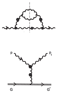
Figure 1: The process of the stimulated scattering soft boson excitation off test gluon through a resummed gluon propagator $\,{}^{\ast}\tilde{\cal D}$, where a vertex of a three-soft-wave interaction is induced by $\,{}^{\ast}\Gamma^{(3)}$. The blob stands for HTL resummation an the double line denotes hard test particle.

Here, the upper figure indicates what the Feynman diagram defines this scattering process – cutting of the effective self-energy graph before inserting a hard bubble along the gluon line.

There is a further process given a contribution of the same order as above-considered. This contribution on the classic language represents the normal Thomson scattering of a wave off thermal particle: a wave with the original frequency $\omega_{\bf p}^{l}$ is a set in oscillatory particle motion, and an oscillating particle radiates a wave with modified frequency $\omega_{{\bf p}_{1}}^{l}$. Diagrammatically this process of scattering is depicted in Fig. 2.

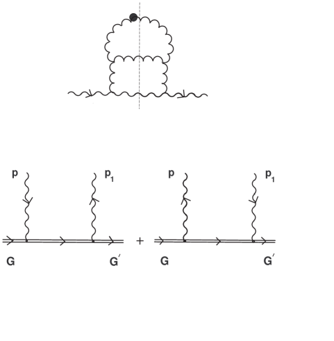
Figure 2: The Compton scattering of soft boson excitations off a test gluon. The upper diagram represents cutting of the effective ‘tadpole’ graph defining this scattering process.

To define contribution of this scattering process to an effective current, account must be taken of influence of the soft random field on a state of color test particle itself. The particle motion in a wave field is described by the system of equations

$$m\frac{d^{2}x^{\mu}}{d\tau^{2}}=gQ^{a}F^{a\mu\nu}(x)\frac{dx_{\nu}}{d\tau},$$ (3.10)

$$\frac{dQ^{a}}{d\tau}=-gf^{abc}\frac{dx^{\mu}}{d\tau}A_{\mu}^{b}(x)Q^{c}.$$

Above, $\tau$ is the proper time. The second equation is known Wong equation. Instead of the expression (3.1) for the color current of a test charge now we must use more general expression

$$j_{Q}^{a\mu}=g\,\frac{dx^{\mu}}{d\tau}Q^{a}(\tau)\delta^{(4)}(x-x(\tau)).$$

The system of equations (3.10) is in a general case very complicated since it describes both the Abelian contribution to radiation connected with the change of trajectory and momentum of the test particle due to interaction with the soft fluctuating gauge field, and the non-Abelian part of the radiation induced by precession of a color spin in the field of the incident wave. Our interest is only with a leading HTL-contribution over coupling constant in considered theory. This makes it possible to simplify the treatment and consider the hard test gluon as moving along the straight line, with constant velocity. In HTL-approximation the QED-like part of the Compton scattering is suppressed, and only the dominant specific non-Abelian contribution survives. The processes of emission and absorption of plasmon is defined by a ‘rotation’ of color vector $Q^{a}=Q^{a}(\tau).$ Thus, in the limit of the accepted accuracy of calculation we need only a minimal extension of the color current of hard test particle

$$j_{Q}^{a\mu}=gv^{\mu}Q^{a}(t){\delta}^{(3)}({\bf x}-{\bf v}t),\quad v^{\mu}=(1,{\bf v}),$$ (3.11)

where a color charge satisfies the Wong equation

$$\frac{dQ^{a}(t)}{dt}=gf^{abc}(v\cdot A^{b}(x))Q^{c}.$$ (3.12)

Here, we turn to a coordinate time.

To derive the oscillations of a color particle, excited by a soft random field and being linear in amplitude of field on the right-hand side of Eq. (3.12) we set the color charge equal to its initial value: $Q^{c}(t_{0})\equiv Q_{0}^{c}$, and we replace a field $A_{\mu}^{b}(x)$ by a free field

$$A_{\mu}^{b}(x)\rightarrow A_{\mu}^{(0)b}(x)=A_{\mu}^{(0)b}(t,{\bf v}t)=\int\!{\rm e}^{-i(v\cdot p)t}A_{\mu}^{(0)b}(p)dp.$$

In this approximation the solution of the Wong equation (3.12) has the form

$$Q^{a}(t)=Q_{0}^{a}+igf^{abc}Q_{0}^{c}\int\!\frac{1}{v\cdot p}\,[\,{\rm e}^{-i(v\cdot p)t}-{\rm e}^{-i(v\cdot p)t_{0}}](v\cdot A^{(0)b}(p))dp.$$ (3.13)

Substituting this expression into (3.11) and turn to Fourier-transformation we obtain additional to (3.6) correction to “starting” current of test particle

$$j_{Q}^{(1)a\mu}(p)=i\,\frac{g^{2}}{(2\pi)^{3}}\,f^{abc}Q_{0}^{c}\int\!\frac{1}{v\cdot p_{1}}\,[\delta(v\cdot(p-p_{1}))-\delta(v\cdot p){\rm e}^{-i(v\cdot p_{1})t_{0}}](v\cdot A^{(0)b}(p_{1}))dp_{1}.$$

Here, the first term in square brackets in integrand defines a resonance condition for the process of the nonlinear Landau damping. The second term is associated with Cherenkov radiation that is absent in our case. In the subsequent discussion all terms in the expressions of (3.13) type, containing initial time will be dropped, because they not contribute to the scattering processes of interest to us.

Adding an obtained current $j_{Q}^{(1)a\mu}(p)$ with current (3.6) we derive complete expression for the first term in the expansion of an effective current in powers of a free field in the leading HTL-approximation

$$\tilde{J}_{Q\mu}^{(1)a}(p)=\frac{g^{2}}{(2\pi)^{3}}\!\int\!\!K_{\mu\mu_{1}}^{aa_{1}}({\bf v}|\,p,-p_{1})A^{(0)\,a_{1}\mu_{1}}(p_{1})\delta(v\cdot(p-p_{1}))dp_{1},$$ (3.14)

where the coefficient function in integrand is defined as

$$K_{\mu\mu_{1}}^{aa_{1}}({\bf v}|\,p,-p_{1})=K_{\mu\mu_{1}}^{aa_{1}b}({\bf v}|\,p,-p_{1})Q_{0}^{b}\equiv if^{aa_{1}b}Q_{0}^{b}\stackrel{{\scriptstyle\scriptscriptstyle{\,(1)}}}{{\displaystyle{K}}}_{\mu\mu_{1}}\!({\bf v}|\,p,-p_{1}),$$ (3.15)

where in turn

$$\stackrel{{\scriptstyle\scriptscriptstyle{\,(1)}}}{{\displaystyle{K}}}_{\mu\mu_{1}}\!({\bf v}|\,p,-p_{1})\equiv\frac{v_{\mu}v_{{\mu}_{1}}}{v\cdot p_{1}}+\!\,^{\ast}\Gamma_{\mu\mu_{1}\nu}(p,-p_{1},-p+p_{1})\,^{\ast}\!\tilde{\cal D}^{\nu\nu^{\prime}}\!(p-p_{1})v_{\nu^{\prime}}.$$ (3.16)

The denominator $v\cdot p_{1}$ in Eq. (3.16) is eikonal, that was expected in an approximation to the small-angle scattering of a high-energy particle. The sense of entering a symbol $\footnotesize{`(1)^{\prime}}$ over $K_{\mu\mu_{1}}\!({\bf v}|\,p,-p_{1})$ will be clear from the context below.

We use the expression of an effective current (3.14) for deriving of desired scattering probability ${\it w}_{2}({\bf v}|\,{\bf p},-{\bf p}_{1})$. The procedure of a calculation of the scattering probabilities with the use of Eqs. (3.8) and (3.9) will be given for general case in Section 6. Here, we present only the final result

$${\it w}_{2}({\bf v}|\,{\bf p},{\bf p}_{1})=N_{c}\,|T({\bf v}|\,{\bf p},-{\bf p}_{1})|^{2}\equiv N_{c}\,|T_{\bf v}({\bf p},-{\bf p}_{1})|^{2},$$ (3.17)

where the function

$$T_{\bf v}({\bf p},-{\bf p}_{1})=g^{2}\!\left[\left(\frac{{\rm Z}_{l}({\bf p})}{2\omega_{\bf p}^{l}}\right)^{\!1/2}\!\!\frac{\tilde{u}^{\mu}(p)}{\sqrt{\bar{u}^{2}(p)}}\right]\!\!\left[\left(\frac{{\rm Z}_{l}({\bf p}_{1})}{2\omega_{{\bf p}_{1}}^{l}}\right)^{\!1/2}\!\!\frac{\tilde{u}^{\mu_{1}}(p_{1})}{\sqrt{\bar{u}^{2}(p_{1})}}\right]\!\stackrel{{\scriptstyle\scriptscriptstyle{\,(1)}}}{{\displaystyle{K}}}_{\mu\mu_{1}}\!({\bf v}|\,p,-p_{1})\Big{|}_{\rm on-shell}$$ (3.18)

represents the scattering amplitude of the nonlinear Landau damping process. The expression (3.17) was obtained in Ref. [3] by a different method, that will be mentioned below.

4 The higher coefficient functions

In previous Section we consider a simpler process of scattering of plasmons off hard thermal particle – the nonlinear Landau damping process. As in pure plasmon-plasmon interaction [1], a calculation of the scattering probability here, reduces to computation of some effective current (Eq. (3.14)) generating this process. We have shown that this effective current apears in the solution of the nonlinear integral field equation (3.2), which defines interacting soft-gluon field $A_{\mu}$ in the form of an expansion in a free field $A_{\mu}^{(0)}=(A_{\mu}^{(0)a})$ and also initial value of a color charge $Q_{0}=(Q_{0}^{a})$. The last circumstance is a new feature of considered problem different from pure plasmon nonlinear dynamics.

Based on results of Paper I and previous section we can rewrite now more general structure of an effective current in the form of a functional expansion in a free field $A_{\mu}^{(0)}$ (and generally speaking, color charge $Q_{0}$) generating the plasmon decay processes and the scattering processes of arbitrary number of plasmons by hard thermal particle

$$\tilde{J}_{\mu}^{({\rm tot})a}[A^{(0)}](p)=\frac{g}{(2\pi)^{3}}\,Q_{0}^{a}v_{\mu}\delta(v\cdot p)+\sum_{s=1}^{\infty}\tilde{J}_{Q\mu}^{(s)a}[A^{(0)}]({\bf v},p)+\sum_{s=2}^{\infty}\tilde{J}_{\mu}^{(s)a}[A^{(0)}](p),$$ (4.1)

where

$$\tilde{J}_{Q\mu}^{(s)a}[A^{(0)}]({\bf v},p)=\frac{1}{s!}\,\frac{g^{s+1}}{(2\pi)^{3}}\!\int\!K_{\mu\mu_{1}\ldots\mu_{s}}^{aa_{1}\ldots a_{s}}({\bf v}|\,p,-p_{1},\ldots,-p_{s})A^{(0)a_{1}\mu_{1}}(p_{1})\ldots A^{(0)a_{s}\mu_{s}}(p_{s})$$

$$\times\delta(v\cdot(p-\sum_{i=1}^{s}p_{i}))\prod_{i=1}^{s}dp_{i},$$

$$\tilde{J}^{(s)a}_{\mu}[A^{(0)}](p)=\frac{1}{s!}\;g^{s-1}\!\!\int\!\!\,^{\ast}\tilde{\Gamma}^{aa_{1}\ldots a_{s}}_{\mu\mu_{1}\ldots\mu_{s}}(p,-p_{1},\ldots,-p_{s})A^{(0)a_{1}\mu_{1}}(p_{1})\ldots A^{(0)a_{s}\mu_{s}}(p_{s})$$

$$\times\delta(p-\sum_{i=1}^{s}p_{i})\prod_{i=1}^{s}dp_{i}.$$

The last sum on the right-hand side of Eq. (4.1) represents an effective current generating plasmon decay processes. The current was studied in detail in Paper I, where a complete algorithm of succesive calculation of coefficient functions $\,{}^{\ast}\tilde{\Gamma}_{\mu\mu_{1}\ldots\mu_{s}}^{aa_{1}\ldots a_{s}}$, was proposed. Now our problem is in constraction of a similar algorithm for calculation of coefficient function $K_{\mu\mu_{1}\ldots\mu_{s}}^{aa_{1}\ldots a_{s}}$. In general the structure of these functions is more complicated and tangled, as compared with $\,{}^{\ast}\tilde{\Gamma}_{\mu\mu_{1}\ldots\mu_{s}}^{aa_{1}\ldots a_{s}}$. This follows from the fact that they represent infinite series in expansion over color charge $Q_{0}$, i.e.

$$K_{\mu\mu_{1}\ldots\mu_{s}}^{aa_{1}\ldots a_{s}}({\bf v}|\,p,-p_{1},\ldots,-p_{s})=\sum_{m=0}^{\infty}K_{\mu\mu_{1}\ldots\mu_{s}}^{aa_{1}\ldots a_{s}\,bb_{1}\ldots b_{m}}({\bf v}|\,p,-p_{1},\ldots,-p_{s})Q_{0}^{b}Q_{0}^{b_{1}}\ldots Q_{0}^{b_{m}},$$ (4.2)

where

$$K_{\mu\mu_{1}\ldots\mu_{s}}^{aa_{1}\ldots a_{s}\,bb_{1}\ldots b_{m}}=\left.\frac{\delta^{m}K^{aa_{1}\ldots a_{s}}_{\mu\mu_{1}\ldots\mu_{s}}}{\delta Q_{0}^{b}\delta Q_{0}^{b_{1}}\ldots\delta Q_{0}^{b_{m}}}\right|_{Q_{0}=0}.$$

Below we discuss a physical meaning of coefficients of this expansion on the example of particular computation. Here, we note that primary consideration will be focussed on computation of the terms linear in $Q_{0}$ in the expansion (4.2) that give leading contribution to the scattering processes of our interest.

The more direct and explicit way of calculation of required coefficient functions $K^{(s)}(\equiv K^{aa_{1}\dots a_{s}}_{\mu\mu_{1}\ldots\mu_{s}})$ was presented in previous section. It is based on usual procedure of computing perturbative solutions of the classical Yang-Mills equation. However such a direct approach for determination of an explicit form of the higher cofficient functions $K^{(s)},\,s>1$, becomes very complicated and as consequence, ineffective. For deriving $K^{(s)}$ we use the approach suggested in Paper I, which was applied to obtain $\!\,{}^{\ast}\tilde{\Gamma}^{(s)}$ with appropriate modification. Remind that this approach is based on simple fact, namely, that the total color current $J^{({\rm tot})\,a\mu}[A]\equiv J^{a\mu}_{NL}[A]+j_{Q}^{a\mu}[A]$, entering into the right-hand side of the field equation (3.2), has two representation: by means of free and interacting fields, which must be equal each other. Thus in representation of free field $A^{(0)}_{\mu}$ the current is defined by Eq. (4.1). To rewrite explicit expression for total current in representation of interacting field we need to define the expansion for current $j_{Q}^{a\mu}[A](p)$ similar to expansion (3.3). For this purpose we write the solution of Eq. (3.12) in the form

$$Q^{a}(t)=U^{ab}(t,t_{0})Q_{0}^{b},$$

where

$$U(t,t_{0})={\rm T}\exp\{-ig\!\int_{t_{0}}^{t}\!(v\cdot A^{a}(\tau,{\bf v}\tau))T^{a}d\tau\}=$$

$$1+\sum_{s=1}^{\infty}(-ig)^{s}\!\int_{t_{0}}^{t}\!d\tau_{1}\int_{t_{0}}^{\tau_{1}}\!d\tau_{2}\ldots\int_{t_{0}}^{\tau_{s-1}}\!d\tau_{s}\,(v\cdot A^{a_{1}}(\tau_{1}))(v\cdot A^{a_{2}}(\tau_{2}))\dots(v\cdot A^{a_{s}}(\tau_{s}))T^{a_{1}}T^{a_{2}}\dots T^{a_{s}}$$

is an evolution operator accounting for the color precession along the parton trajectory. Here, $(T^{a})^{bc}=-if^{abc}$, and in the last line we set $A^{a}_{\mu}({\tau})\equiv A^{a}_{\mu}(\tau,{\bf v}\tau)$. Using this form of the solution of the Wong equation, we can present a current $j_{Q}^{a\mu}[A](p)$ in the form

$$j_{Q}^{a\mu}[A](p)=\frac{g}{(2\pi)^{3}}\,Q_{0}^{a}v^{\mu}\delta(v\cdot p)+\frac{g}{(2\pi)^{3}}\,v^{\mu}\!\!\int\!{\rm e}^{i(v\cdot p)t}[U(t,t_{0})-1]^{ab}Q_{0}^{b}\,\frac{dt}{2\pi}.$$ (4.3)

Adding the obtained expression with nonlinear current $(\ref{eq:3e})$, we derive a total expression for current in the representation of an interacting field

$$J_{\mu}^{({\rm tot})a}[A](p)=J_{NL\,\mu}^{a}[A](p)+j_{Q\,\mu}^{a}[A](p)$$

$$=\sum_{s=2}^{\infty}\frac{1}{s!}\,g^{s-1}\!\!\int\!\,^{\ast}\Gamma^{aa_{1}\ldots a_{s}}_{\mu\mu_{1}\ldots\mu_{s}}(p,-p_{1},\ldots,-p_{s})A^{a_{1}\mu_{1}}(p_{1})A^{a_{2}\mu_{2}}(p_{2})\ldots A^{a_{s}\mu_{s}}(p_{s})\delta(p-\sum_{i=1}^{s}p_{i})\prod_{i=1}^{s}dp_{i}$$ (4.4)

$$+\,\frac{g}{(2\pi)^{3}}\,Q_{0}^{a}v_{\mu}\delta(v\cdot p)+v_{\mu}\sum_{s=1}^{\infty}\frac{g^{s+1}}{(2\pi)^{3}}\int\!\frac{1}{(v\cdot(p_{1}+\ldots+p_{s}))(v\cdot(p_{2}+\ldots+p_{s}))\ldots(v\cdot p_{s})}$$

$$\times(v\cdot A^{a_{1}}(p_{1}))\ldots(v\cdot A^{a_{s}}(p_{s}))\delta(v\cdot(p-\sum_{i=1}^{s}p_{i}))\prod_{i=1}^{s}dp_{i}\,(T^{a_{1}}\ldots T^{a_{s}})^{ab}Q_{0}^{b}.$$

Here, in derivation of two last lines in Eq. (4.4) we drop all terms containing initial time $t_{0}$. The interacting fields on the right-hand side of Eq. (4.4) are defined by expansion

$$A^{a\mu}(p)=A^{(0)\,a\mu}(p)-\!\,^{\ast}\tilde{\cal D}^{\mu\mu^{\prime}}(p)\tilde{J}^{({\rm tot})\,a}_{\mu^{\prime}}[A^{(0)}](p),$$ (4.5)

where the current $\tilde{J}^{({\rm tot})a}_{\mu^{\prime}}$ is defined by Eq. (4.1). Thus we have two different representations for total color current: Eqs. (4.1) and (4.4), which must be equal each other

$$\tilde{J}^{({\rm tot})\,a}_{\mu}[A^{(0)}](p)=J^{({\rm tot})\,a}_{\mu}[A](p).$$ (4.6)

Substitution of Eq. (4.5) into the right-hand side of Eq. (4.6) turns this equation into identity. As for pure plasmon-plasmon scattering [1], for derivation of required coefficient functions $K^{(s)}$ it should be differentiated left- and right-hand sides of equality (4.6) with respect to free field $A_{\mu}^{(0)}$ considering Eq. (4.4) for differentiation on the right-hand side, and set $A_{\mu}^{(0)}=0$ after all calculations. However in this case it is necessary to add differentiation with respect to initial color charge $Q_{0}$ to differentiation with respect to free field $A_{\mu}^{(0)}$, and it should be added the condition $Q_{0}=0$ to condition $A_{\mu}^{(0)}=0$ after all calculations. Below we shall give a few examples.

The second differentiation of a total current yields

$$\left.\frac{\delta^{2}\!J^{({\rm tot})\,a}_{\mu}[A](p)}{\delta Q_{0}^{b}\,\delta A^{(0)a_{1}\mu_{1}}(p_{1})}\right|_{A^{(0)}=0,\,Q_{0}=0}=\left.\frac{\delta K_{\mu\mu_{1}}^{aa_{1}}({\bf v}|\,p,-p_{1})}{\delta Q_{0}^{b}}\right|_{Q_{0}=0}\!\delta(v\cdot(p-p_{1}))$$ (4.7)

$$=(T^{a_{1}})^{ab}\stackrel{{\scriptstyle\scriptscriptstyle{\,(1)}}}{{\displaystyle{K}}}_{\mu\mu_{1}}({\bf v}|\,p,-p_{1})\,\delta(v\cdot(p-p_{1})),$$

where Lorentz tensor $\stackrel{{\scriptstyle\scriptscriptstyle{\,(1)}}}{{\displaystyle{K}}}_{\mu\mu_{1}}$ is defined by Eq. (3.16) and represents a sum of two different contribution depicted in Figs. 1 and 2.

A more nontrivial example arises in calculation of the next derivative. It defines the process of nonlinear interaction of three wave with hard test particle

$$\left.\frac{\delta^{3}\!J^{({\rm tot})\,a}_{\mu}[A](p)}{\delta Q_{0}^{b}\,\delta A^{(0)a_{1}\mu_{1}}(p_{1})\delta A^{(0)a_{2}\mu_{2}}(p_{2})}\right|_{A^{(0)}=0,\,Q_{0}=0}=\left.\frac{\delta K_{\mu\mu_{1}\mu_{2}}^{aa_{1}a_{2}}({\bf v}|\,p,-p_{1},-p_{2})}{\delta Q_{0}^{b}}\right|_{Q_{0}=0}\!\delta(v\cdot(p-p_{1}-p_{2}))$$ (4.8)

$$=[(T^{a_{1}}T^{a_{2}})^{ab}\stackrel{{\scriptstyle\scriptscriptstyle{\,(1)}}}{{\displaystyle{K}}}_{\mu\mu_{1}\mu_{2}}\!({\bf v}|\,p,-p_{1},-p_{2})+(T^{a_{2}}T^{a_{1}})^{ab}\stackrel{{\scriptstyle\scriptscriptstyle{\,(1)}}}{{\displaystyle{K}}}_{\mu\mu_{2}\mu_{1}}\!({\bf v}|\,p,-p_{2},-p_{1})]\,\delta(v\cdot(p-p_{1}-p_{2})).$$

The color factor on the right-hand side of Eq. (4.8) are multiplied by pure kinematical coefficients, which we will call partial coefficient functions, and are defined as follows

$$\stackrel{{\scriptstyle\scriptscriptstyle{\,(1)}}}{{\displaystyle{K}}}_{\mu\mu_{1}\mu_{2}}\!({\bf v}|\,p,-p_{1},-p_{2})=\frac{v_{\mu}v_{\mu_{1}}v_{\mu_{2}}}{(v\cdot p_{2})(v\cdot(p_{1}+p_{2}))}$$

$$+\,\frac{v_{\mu}v_{\nu}}{v\cdot(p_{1}+p_{2})}\,^{\ast}\tilde{\cal D}^{\nu\nu^{\prime}}(p_{1}+p_{2})\,^{\ast}\Gamma_{\nu^{\prime}\mu_{1}\mu_{2}}(p_{1}+p_{2},-p_{1},-p_{2})$$ (4.9)

$$-\,^{\ast}\Gamma_{\mu\mu_{1}\mu_{2}\nu}(p,-p_{1},-p_{2},-p+p_{1}+p_{2})\,^{\ast}\tilde{\cal D}^{\nu\nu^{\prime}}(p-p_{1}-p_{2})v_{{\nu}^{\prime}}$$

$$+\,^{\ast}\Gamma_{\mu\mu_{1}\nu}(p,-p_{1},-p+p_{1})\,^{\ast}\tilde{\cal D}^{\nu\nu^{\prime}}(p-p_{1})\stackrel{{\scriptstyle\scriptscriptstyle{\,(1)}}}{{\displaystyle{K}}}_{\nu^{\prime}\mu_{2}}\!({\bf v}|\,p-p_{1},-p_{2})$$

$$-\,^{\ast}\Gamma_{\mu\nu\lambda}(p,-p+p_{1}+p_{2},-p_{1}-p_{2})\!\,^{\ast}\tilde{\cal D}^{\nu\nu^{\prime}}(p-p_{1}-p_{2})v_{{\nu}^{\prime}}\!\,^{\ast}\tilde{\cal D}^{\lambda\lambda^{\prime}}(p_{1}+p_{2})\!\,^{\ast}\Gamma_{\lambda^{\prime}\mu_{1}\mu_{2}}(p_{1}+p_{2},-p_{1},-p_{2}).$$

Here, the fuction $\stackrel{{\scriptstyle\scriptscriptstyle{\,(1)}}}{{\displaystyle{K}}}_{\mu\mu_{1}\mu_{2}}$ consists of five terms different in structure, whose diagram interpretation was presented on Fig. 3.

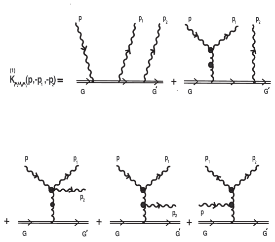
Figure 3: The process of the stimulated scattering of third soft boson excitations off hard test parton.

Above-mentioned two examples suggest on that coefficient functions $(\delta K_{\mu\mu_{1}\ldots\mu_{s}}^{aa_{1}\ldots a_{s}}/\delta Q_{0}^{b})_{Q_{0}=0}$ have a color structure, similar to color structure of effective amplitudes $\,{}^{\ast}\tilde{\Gamma}^{aa_{1}\ldots a_{s+1}}_{\mu\mu_{1}\ldots\mu_{s+1}}$, and thus coincide with color structure of usual HTL-amplitudes, first proposed by Braaten and Pisarski in Ref. [2] for an arbitrary number of external soft-gluon legs. To test this assumption we calculate a next derivative with respect to free field $A^{(0)}_{\mu}$:

$$\left.\frac{\delta^{4}\!J^{({\rm tot})\,a}_{\mu}[A](p)}{\delta Q_{0}^{b}\,\delta A^{(0)a_{1}\mu_{1}}(p_{1})\delta A^{(0)a_{2}\mu_{2}}(p_{2})\delta A^{(0)a_{3}\mu_{3}}(p_{3})}\right|_{A^{(0)}=0,\,Q_{0}=0}$$ (4.10)

$$=\left.\frac{\delta K_{\mu\mu_{1}\mu_{2}\mu_{3}}^{aa_{1}a_{2}a_{3}}({\bf v}|\,p,-p_{1},-p_{2},-p_{3})}{\delta Q_{0}^{b}}\right|_{Q_{0}=0}\!\delta(v\cdot(p-p_{1}-p_{2}-p_{3}))$$

$$=[(T^{a_{1}}T^{a_{2}}T^{a_{3}})^{ab}\stackrel{{\scriptstyle\scriptscriptstyle{\,(1)}}}{{\displaystyle{K}}}_{\mu\mu_{1}\mu_{2}\mu_{3}}\!({\bf v}|\,p,-p_{1},-p_{2},-p_{3})+({\rm perm.}\,1,2,3)]\,\delta(v\cdot(p-p_{1}-p_{2}-p_{3})),$$

where

$$\stackrel{{\scriptstyle\scriptscriptstyle{\,(1)}}}{{\displaystyle{K}}}_{\mu\mu_{1}\mu_{2}\mu_{3}}\!({\bf v}|\,p,-p_{1},-p_{2},-p_{3})=\frac{v_{\mu}}{v\cdot(p_{1}+p_{2}+p_{3})}\left\{\frac{v_{\mu_{1}}v_{\mu_{2}}v_{\mu_{3}}}{(v\cdot p_{2})(v\cdot(p_{2}+p_{3}))}\right.$$

$$+\,v_{\nu}\!\,^{\ast}\tilde{\cal D}^{\nu\nu^{\prime}}\!(p_{1}+p_{2}+p_{3})\,^{\ast}\Gamma_{\nu^{\prime}\mu_{1}\mu_{3}\mu_{2}}(p_{1}+p_{2}+p_{3},-p_{1},-p_{3},-p_{2})$$

$$+\,\frac{1}{v\cdot p_{2}}\,v_{\nu}\!\,^{\ast}\tilde{\cal D}^{\nu\nu^{\prime}}\!(p_{1}+p_{3})\,^{\ast}\Gamma_{\nu^{\prime}\mu_{1}\mu_{3}}(p_{1}+p_{3},-p_{1},-p_{3})v_{\mu_{2}}$$

$$\left.-\,\frac{1}{v\cdot(p_{2}+p_{3})}\,v_{\nu}\!\,^{\ast}\tilde{\cal D}^{\nu\nu^{\prime}}\!(p_{2}+p_{3})\,^{\ast}\Gamma_{\nu^{\prime}\mu_{2}\mu_{3}}(p_{2}+p_{3},-p_{2},-p_{3})v_{\mu_{1}}\right\}$$

$$-\,\Bigl{\{}\!\,^{\ast}\Gamma_{\mu\mu_{1}\nu}(p,-p_{1},-p+p_{1})\,^{\ast}\tilde{\cal D}^{\nu\nu^{\prime}}\!(p-p_{1})\stackrel{{\scriptstyle\scriptscriptstyle{\,(1)}}}{{\displaystyle{K}}}_{\nu^{\prime}\mu_{2}\mu_{3}}\!({\bf v}|\,p-p_{1},-p_{2},-p_{3})$$

$$+\!\,^{\ast}\Gamma_{\mu\nu\lambda}(p,\!-p_{3},\!-p+p_{3})\!\,^{\ast}\!\tilde{\cal D}^{\nu\nu^{\prime}}\!(p_{3})\!\!\stackrel{{\scriptstyle\scriptscriptstyle{\,(1)}}}{{\displaystyle{K}}}_{\nu^{\prime}\mu_{3}}\!\!({\bf v}|\,p\!-p_{1}\!-p_{2},\!-p_{3})\!\,^{\ast}\!\tilde{\cal D}^{\lambda\lambda^{\prime}}\!(p_{1}+p_{2})\!\,^{\ast}\Gamma_{\lambda^{\prime}\mu_{1}\mu_{2}}(p_{1}+p_{2},\!-p_{1},\!-p_{2})$$

$$+\,^{\ast}\Gamma_{\mu\nu\lambda}(p,-p+p_{1}+p_{2}+p_{3},-p_{1}-p_{2}-p_{3})\!\,^{\ast}\tilde{\cal D}^{\nu\nu^{\prime}}\!(p-p_{1}-p_{2}-p_{3})v_{{\nu}^{\prime}}$$

$$\times\!\,^{\ast}\tilde{\cal D}^{\lambda\lambda^{\prime}}\!(p_{1}+p_{2}+p_{3})\!\,^{\ast}\Gamma_{\lambda^{\prime}\mu_{1}\mu_{2}\mu_{3}}(p_{1}+p_{2}+p_{3},-p_{1},-p_{2},-p_{3})\Bigr{\}}$$

$$-\,\Bigl{\{}\!\,^{\ast}\Gamma_{\mu\mu_{1}\mu_{2}\nu}(p,-p_{1},-p_{2},-p+p_{1}+p_{2})\,^{\ast}\tilde{\cal D}^{\nu\nu^{\prime}}\!(p-p_{1}-p_{2})\!\stackrel{{\scriptstyle\scriptscriptstyle{\,(1)}}}{{\displaystyle{K}}}_{\nu^{\prime}\mu_{3}}\!({\bf v}|\,p-p_{1}-p_{2},-p_{3})$$

$$+\,^{\ast}\Gamma_{\mu\lambda\mu_{3}\nu}(p,-p_{1}-p_{2},-p_{3},-p+p_{1}+p_{2}+p_{3})\!\,^{\ast}\tilde{\cal D}^{\nu\nu^{\prime}}\!(p-p_{1}-p_{2}-p_{3})v_{{\nu}^{\prime}}$$

$$\times\!\,^{\ast}\tilde{\cal D}^{\lambda\lambda^{\prime}}\!(p_{1}+p_{2})\!\,^{\ast}\Gamma_{\lambda^{\prime}\mu_{1}\mu_{2}}(p_{1}+p_{2},-p_{1},-p_{2})$$

$$+\,^{\ast}\Gamma_{\mu\mu_{1}\lambda\nu}(p,-p_{1},-p_{2}-p_{3},-p+p_{1}+p_{2}+p_{3})\!\,^{\ast}\tilde{\cal D}^{\nu\nu^{\prime}}\!(p-p_{1}-p_{2}-p_{3})v_{{\nu}^{\prime}}$$

$$\times\!\,^{\ast}\tilde{\cal D}^{\lambda\lambda^{\prime}}\!(p_{2}+p_{3})\!\,^{\ast}\Gamma_{\lambda^{\prime}\mu_{2}\mu_{3}}(p_{2}+p_{3},-p_{2},-p_{3})\Bigr{\}}$$

$$-\,^{\ast}\Gamma_{\mu\mu_{1}\mu_{2}\mu_{3}\nu}(p,-p_{1},-p_{2},-p_{3},-p+p_{1}+p_{2}+p_{3})\,^{\ast}\tilde{\cal D}^{\nu\nu^{\prime}}\!(p-p_{1}-p_{2}-p_{3})v_{{\nu}^{\prime}}.$$

The right-hand side of this expression is represented for convenience as a sum of four groups of terms defined by derivation of currents $j_{Q\mu}^{a},\,J_{\mu}^{(2)a},\,J_{\mu}^{(3)a}$ and $J_{\mu}^{(4)a}$ (Eqs. (3.2), (3.3)), respectively. Thus one can state that a color structure of the first term in the expansion of arbitrary coefficient function (4.2) linear over color charge $Q_{0}^{b}$, entirely coincides with the color structure of usual $(s+2)$-gluon HTL-amplitudes.

In closing we consider the problem on physical meaning of higher power of color charge $Q_{0}$ in the expansion of coefficient functions $K_{\mu\mu_{1}\ldots\mu_{s}}^{aa_{1}\ldots a_{s}}$ (Eq. (4.2)). For this purpose we calculate the second derivative of the expression (4.7) with respect to $Q_{0}$

$$\left.\frac{\delta^{3}\!J^{({\rm tot})\,a}_{\mu}[A](p)}{\delta Q_{0}^{b}\,\delta Q_{0}^{b_{1}}\,\delta A^{(0)a_{1}\mu_{1}}(p_{1})}\right|_{A^{(0)}=0,\,Q_{0}=0}=\frac{g^{2}}{(2\pi)^{3}}\left.\frac{\delta^{2}K_{\mu\mu_{1}}^{aa_{1}}({\bf v}|\,p,-p_{1})}{\delta Q_{0}^{b}\,\delta Q_{0}^{b_{1}}}\right|_{Q_{0}=0}\!\delta(v\cdot(p-p_{1}))$$

$$=\frac{g^{2}}{(2\pi)^{3}}\,\{T^{b},T^{b_{1}}\}^{aa_{1}}\stackrel{{\scriptstyle\scriptscriptstyle{\,(2)}}}{{\displaystyle{K}}}_{\mu\mu_{1}}\!({\bf v}|\,p,-p_{1})\,\delta(v\cdot(p-p_{1})),$$

where

$$\stackrel{{\scriptstyle\scriptscriptstyle{\,(2)}}}{{\displaystyle{K}}}_{\mu\mu_{1}}\!({\bf v}|\,p,-p_{1})=\int\!\bigg{\{}\frac{v_{\mu}v_{\mu_{1}}}{(v\cdot p_{1})(v\cdot(p_{1}+p_{1}^{\prime}))}\,(v_{\nu}\!\,^{\ast}\tilde{\cal D}^{\nu\nu^{\prime}}\!(p_{1}^{\prime})v_{\nu^{\prime}})$$

$$-\,\frac{v_{\mu}v_{\nu}}{v\cdot(p_{1}+p_{1}^{\prime})}\,^{\ast}\tilde{\cal D}^{\nu\nu^{\prime}}\!(p_{1}+p_{1}^{\prime})\!\stackrel{{\scriptstyle\scriptscriptstyle{\,(1)}}}{{\displaystyle{K}}}_{{\nu}^{\prime}\mu_{1}}\!({\bf v}|\,p_{1}+p_{1}^{\prime},-p_{1})$$ (4.11)

$$+\,^{\ast}\Gamma_{\mu\nu_{1}\nu_{2}\mu_{1}}(p,-p_{1}^{\prime},-p+p_{1}+p_{1}^{\prime},-p_{1})\,^{\ast}\tilde{\cal D}^{\nu_{1}\nu_{1}^{\prime}}(p_{1}^{\prime})v_{{\nu_{1}}^{\prime}}\!\,^{\ast}\tilde{\cal D}^{\nu_{2}\nu_{2}^{\prime}}(p-p_{1}-p_{1}^{\prime})v_{{\nu_{2}}^{\prime}}$$

$$+\,^{\ast}\Gamma_{\mu\nu_{1}\nu_{2}}(p,-p_{1}^{\prime},-p+p_{1}^{\prime})\,^{\ast}\tilde{\cal D}^{\nu_{1}\nu_{1}^{\prime}}(p_{1}^{\prime})v_{{\nu}_{1}^{\prime}}\!\,^{\ast}\tilde{\cal D}^{\nu_{2}\nu_{2}^{\prime}}(p-p_{1}^{\prime})\!\stackrel{{\scriptstyle\scriptscriptstyle{\,(1)}}}{{\displaystyle{K}}}_{{\nu}^{\prime}_{2}\mu_{1}}\!({\bf v}|\,p-p_{1}^{\prime},-p_{1})\bigg{\}}\,\delta(v\cdot p_{1}^{\prime})dp_{1}^{\prime}.$$

It is easy to check by direct calculation that partial coefficient function $\stackrel{{\scriptstyle\scriptscriptstyle{\,(2)}}}{{\displaystyle{K}}}_{\mu\mu_{1}}\!({\bf v}|\,p,-p_{1})$ is symmetric relative to permutation $p\leftrightarrow-p_{1}$, as it must be. The diagrammatic interpretation of different terms in the right-hand side of Eq. (4.11) is presented on Fig. 4.

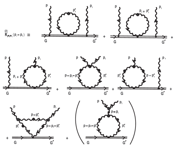
Figure 4: The soft one-loop corrections to nonlinear Landau damping process.

The presence of resonance factor $\delta(v\cdot(p-p_{1}))$ and integration over loop momentum $p_{1}^{\prime}$ points to the fact that here, we are concerned with soft one-loop correction to nonlinear Landau damping process, that is suppressed by power of $g^{2}$ as compared with tree approximation (3.15), (3.16). We note specially that the region of integration in loops is restricted by cone $v\cdot p_{1}^{\prime}=0$. The contribution

$$\int\!\!\,^{\ast}\Gamma_{\mu_{1}\mu_{2}\nu}(p,-p_{1},-p+p_{1})\,^{\ast}\tilde{\cal D}^{\nu\nu^{\prime}}\!(p-p_{1})\,^{\ast}\Gamma_{\nu\lambda\sigma}(p-p_{1},-p_{1}^{\prime},-p+p_{1}+p_{1}^{\prime})$$

$$\times\,^{\ast}\tilde{\cal D}^{\lambda\lambda^{\prime}}\!(p_{1}^{\prime})v_{{\lambda}^{\prime}}\,^{\ast}\tilde{\cal D}^{\sigma\sigma^{\prime}}\!(p-p_{1}-p_{1}^{\prime})v_{\sigma^{\prime}}\,\delta(v\cdot p_{1}^{\prime})\,\delta(v\cdot(p-p_{1}))dp_{1}^{\prime}$$

corresponds to the last term (in parenthesis) in Fig. 4. By virtue of a property of three-gluon HTL-amplitude: $\!\,{}^{\ast}\Gamma_{\mu\mu_{1}\mu_{2}}(p,-p_{1},-p_{2})=-\!\,^{\ast}\Gamma_{\mu\mu_{2}\mu_{1}}(p,-p_{2},-p_{1})$, the integrand is odd under the interchange of $p_{1}^{\prime}\rightarrow p-p_{1}-p_{1}^{\prime}$ and integrates to zero.

It is clear that higher powers in $Q_{0}$ in the expansion (4.2) is associated with soft loop corrections of higher orders, and they are suppressed relative to linear term $(\delta\!K_{\mu\mu_{1}}^{aa_{1}}/\delta Q_{0}^{b})_{Q_{0}=0}$ as $(g^{2})^{2}$ etc. The partial coefficients functions $\stackrel{{\scriptstyle\scriptscriptstyle{\,(r)}}}{{\displaystyle{K}}}_{\mu\mu_{1}}\!({\bf v}|\,p,-p_{1}),\,r\geq 2$ (more precisely, an effective current connected with them) can be interpretated as “dressing” of initial current of hard test color particle or simple of a particle caused by interaction of this current with hot bath. For derivation of total probability of the process of the nonlinear Landau damping (process of elastic scattering for $n=0$ in Eq. (2.8)), we must, generally speaking, summarize a series in expansion in a color charge degree $Q_{0}$. It can be considered as a replacement of initial test particle by some effective quasiparticle on which in fact the scattering process of soft-gluon wave takes place. It is successfully that even in the case of highly excited gluon plasma (see next section) soft loop corrections are suppressed and therefore in leading order we can neglect by it.

Finally we point to one interest relation, which exists between partial coefficient functions $\stackrel{{\scriptstyle\scriptscriptstyle{\,(2)}}}{{\displaystyle{K}}}_{\mu\mu_{1}}\!({\bf v}|\,p,-p_{1}),\,\stackrel{{\scriptstyle\scriptscriptstyle{\,(1)}}}{{\displaystyle{K}}}_{\mu\mu_{1}\mu_{2}}\!({\bf v}|\,p,-p_{1},-p_{2})$ and four – soft-gluon effective subamplitude $\!\,{}^{\ast}\tilde{\Gamma}_{\mu\mu_{1}\mu_{2}\mu_{3}}(p,-p_{1},-p_{2},-p_{3})$ defined by equation (I.5.6). For its derivation we contract the expression (4.9) with ${}^{\ast}\tilde{\cal D}^{\mu_{1}\mu_{1}^{\prime}}(p_{1})v_{\mu_{1}^{\prime}}$, integrate over $dp_{1}$ and replace variables $p_{1}\rightarrow p_{1}^{\prime},\,p_{2}\rightarrow p_{1}$ and indices: $\mu_{1}\rightarrow\nu,\,\mu_{2}\rightarrow\mu_{1}$ etc. After some algebraic transformations with use of Eq. (I.5.12) and explicit form $\stackrel{{\scriptstyle\scriptscriptstyle{\,(2)}}}{{\displaystyle{K}}}_{\mu\mu_{1}}\!({\bf v}|\,p,-p_{1})$ we obtain desired relation

$$\stackrel{{\scriptstyle\scriptscriptstyle{\,(2)}}}{{\displaystyle{K}}}_{\mu\mu_{1}}\!({\bf v}|\,p,-p_{1})=-\int\!\frac{v_{\mu}v_{\mu_{1}}}{(v\cdot(p_{1}+p_{1}^{\prime}))^{2}}\,(v_{\nu}\!\,^{\ast}\tilde{\cal D}^{\nu\nu^{\prime}}\!(p+p_{1}^{\prime})v_{\nu^{\prime}})\,\delta(v\cdot p_{1}^{\prime})dp_{1}^{\prime}$$

$$+\int\!\stackrel{{\scriptstyle\scriptscriptstyle{\,(1)}}}{{\displaystyle{K}}}_{\mu\nu\mu_{1}}\!({\bf v}|\,p,-p_{1}^{\prime},-p_{1})\,^{\ast}\tilde{\cal D}^{\nu\nu^{\prime}}\!(p_{1}^{\prime})v_{\nu^{\prime}}\,\delta(v\cdot p_{1}^{\prime})dp_{1}^{\prime}$$ (4.12)

$$+\,\frac{1}{2}\!\int\!\!\,^{\ast}\tilde{\Gamma}_{\mu\nu\mu_{1}\lambda}(p,-p_{1}^{\prime},-p_{1},-p+p_{1}+p_{1}^{\prime})\,^{\ast}\tilde{\cal D}^{\lambda\lambda^{\prime}}\!(p-p_{1}-p_{1}^{\prime})v_{{\lambda}^{\prime}}\,^{\ast}\tilde{\cal D}^{\nu\nu^{\prime}}\!(p_{1}^{\prime})v_{\nu^{\prime}}\,\delta(v\cdot p_{1}^{\prime})dp_{1}^{\prime}.$$

The existence of such relation is not difficult for understanding by using diagramm representation of the functions entering in it. Thus the second term on the right-hand side of Eq. (4.12) corresponds to procedure of closing one of soft plasmon legs in Fig. 3 (in our case the legs with soft momentum $p_{1}$) on hard test particle, as it depicted in Fig. 4. The last term on the right-hand side of (4.12) is connected with closing two external soft legs of diagramm on the left hand side in Fig. I.1 and attaching hard line of test particle to close loop. The physical meaning of the first term on the right-hand side of (4.12) is less clear (see however below). It is evident that relation of such a kind exists and for higher partical coefficient function and effective subamplitudes. It can be supposed that they are a consequence of gauge invariance (more precisely, covariance) of total effective current (4.1) with respect to gauge transformations concerned both a field $A_{\mu}^{(0)a}(p)$ and a color charge $Q_{0}^{a}$. We still return to analysis of relation (4.12) in our next work [44] in consideration of the process of nonlinear Landau damping with regard to rescattering of test particle off another hard test particle, where a reason of appearing the first term on the right-hand side of (4.12) becomes more explicit.

5 Characteristic amplitudes of the soft gluon field

In this Section we shall estimate for which typical amplitude of the soft gluon field, the contribution of the nonlinear Landau damping process to a generalized decay and regeneration rates, $\Gamma_{\rm d}[N_{\bf p}^{l}]$ and $\Gamma_{\rm i}[N_{\bf p}^{l}]$, will be leading and for which value all terms in the expansions (2.2) will be of the same order in $g$. As a preliminary we define a general expression for scattering probability ${\it w}_{2n+2}={\it w}_{2n+2}({\bf v}|\,{\bf p},{\bf p}_{1},\ldots,{\bf p}_{n};{\bf p}_{n+1},\ldots,{\bf p}_{2n+1})$. Since the basic moments of computation of the scattering probability by a hard particle repeat reasoning used for deriving the scattering probability in pure plasmon-plasmon scattering in Paper I, Section 4, here, we restrict our consideration to brief scheme of calculation of ${\it w}_{2n+2}$.

Initial expression for deriving ${\it w}_{2n+2}$ is Eq. (3.8) defining the emitted radiant power of the longitudinal waves ${\cal I}^{l}$. The current entering into correlation function is given by

$$\tilde{J}_{Q\,\mu}^{a}[A^{(0)}](p)=\frac{g}{(2\pi)^{3}}\,Q_{0}^{a}v_{\mu}\delta(v\cdot p)+\sum_{s=1}^{\infty}\tilde{J}_{Q\mu}^{(s)a}[A^{(0)}]({\bf v},p),$$ (5.1)

where

$$\tilde{J}_{Q\mu}^{(s)a}[A^{(0)}]({\bf v},p)=\frac{1}{s!}\,\frac{g^{s+1}}{(2\pi)^{3}}\int\!K_{\mu\mu_{1}\ldots\mu_{s}}^{aa_{1}\ldots a_{s}}({\bf v}|\,p,-p_{1},\ldots,-p_{s})A^{(0)a_{1}\mu_{1}}(p_{1})\ldots A^{(0)a_{s}\mu_{s}}(p_{s})$$

$$\times\delta(v\cdot(p-\sum_{i=1}^{s}p_{i}))\prod_{i=1}^{s}dp_{i}.$$

Here, in the coefficient functions $K^{(s)}$ we leave only the term leading order in $g$ in the expansion (4.2), i.e. linear in color charge $Q_{0}$

$$K_{\mu\mu_{1}\ldots\mu_{s}}^{aa_{1}\ldots a_{s}}({\bf v}|\,p,-p_{1},\ldots,-p_{s})\simeq K_{\mu\mu_{1}\ldots\mu_{s}}^{aa_{1}\ldots a_{s}\,b}({\bf v}|\,p,-p_{1},\ldots,-p_{s})Q_{0}^{b}.$$

In substitution of the current expansion (5.1) into a correlation function in integrand of Eq. (3.8) we face the product of two series. As in deriving probability of plasmon decays, in this product it is necessary to leave only a sum of a product of terms having the same order in power of a potential $A_{\mu}^{(0)}$. In this case only a desired $\delta$-function entering to integration measure $\int d{\cal T}^{(2n+1)}$, defining the generalized resonance condition (2.9), arise. Thus the emitted radiant power (3.8), taking into account emission caused by the processes of scattering plasmons off hard test particle, can be represented in the form of expansion

$${\cal I}^{l}={\cal I}^{l(0)}+\sum_{s=1}^{\infty}{\cal I}^{l(s)},$$

where

$${\cal I}^{l(0)}=-\,\frac{g^{2}}{2(2\pi)^{2}}\!\left(\int\!\frac{d|{\bf k}|}{2\pi^{2}}|{\bf k}|^{2}f_{\bf k}\right)\!\int\!\frac{d\Omega_{\bf v}}{4\pi}\!\int\!d\omega\,|\omega|\!\int\!\!d{\bf p}\,(v_{\mu}\tilde{Q}^{\mu\mu^{\prime}}(p)v_{{\mu}^{\prime}})\delta(v\cdot p)\delta({\rm Re}\,^{\ast}\!\Delta^{-1\,l}(p)),$$

and

$${\cal I}^{l\,(s)}=-\,\frac{1}{4\pi}\left(\int\!\frac{d|{\bf k}|}{2\pi^{2}}|{\bf k}|^{2}f_{\bf k}\right)\lim\limits_{\tau\rightarrow\infty}\frac{1}{\tau}\,\frac{g^{2s+2}}{(s!)^{2}}\left(\frac{1}{N_{c}}\!\int\!dQ\,Q_{0}^{b}Q_{0}^{b^{\prime}}\right)$$ (5.2)

$$\times\!\int\!\frac{d\Omega_{\bf v}}{4\pi}\int\!dp\,|\omega|\,\delta^{aa^{\prime}}\tilde{Q}^{\mu\mu^{\prime}}(p)K^{\ast\,aa_{1}\ldots a_{s}b}_{\mu\mu_{1}\ldots\mu_{s}}({\bf v}|\,p,-p_{1},\ldots,-p_{s})K^{a^{\prime}a^{\prime}_{1}\ldots a^{\prime}_{s}b^{\prime}}_{\mu^{\prime}\mu^{\prime}_{1}\ldots\mu^{\prime}_{s}}({\bf v}|\,p,-p_{1}^{\prime},\ldots,-p_{s}^{\prime})$$

$$\times\langle A^{\ast(0)a_{1}\mu_{1}}(p_{1})\ldots A^{\ast(0)a_{s}\mu_{s}}(p_{s})A^{(0)a^{\prime}_{1}\mu^{\prime}_{1}}(p^{\prime}_{1})\ldots A^{(0)a^{\prime}_{s}\mu^{\prime}_{s}}(p^{\prime}_{s})\rangle\delta(v\cdot(p-\sum_{i=1}^{s}p_{i}))$$

$$\times\delta(v\cdot(p-\sum_{i=1}^{s}p^{\prime}_{i}))\delta({\rm Re}\,^{\ast}\!\Delta^{\!-1\,l}(p))\!\prod_{i=1}^{s}dp_{i}dp_{i}^{\prime}.$$

The first term ${\cal I}^{(0)}$ is connected with Cherenkov radiation (the linear Landau damping) which is kinematically forbidden in hot gluon plasma and therefore, this term can be setting zero. Let us consider the remaining terms ${\cal I}^{l(s)},\,s\geq 1$.

The integration over color charge in (5.2) is trivial. Furthermore we write out decoupling of the $2s$th-order correlator on the right-hand side of Eq. (5.2) in terms of pair correlators by rule defined by us in Paper I. Employing a condensed notion, $A_{1}\equiv A_{\mu_{1}}^{(0)a_{1}}(p_{1})$ etc, we have

$$\langle A^{\ast(0)}_{1}\ldots A^{\ast(0)}_{s}A^{(0)}_{1^{\prime}}\ldots A^{(0)}_{s^{\prime}}\rangle=(s!)^{2}\langle A^{\ast(0)}_{1}A^{(0)}_{1^{\prime}}\rangle\ldots\langle A^{\ast(0)}_{s}A^{(0)}_{s^{\prime}}\rangle$$ (5.3)

$$=(s!)^{2}\prod_{i=1}^{s}\delta^{a_{i}a_{i}^{\prime}}\tilde{Q}^{\mu_{i}\mu_{i}^{\prime}}(p_{i})I^{l}(p_{i})\delta(p_{i}-p_{i}^{\prime})$$

$$\simeq(s!)^{2}\prod_{i=1}^{s}\delta^{a_{i}a_{i}^{\prime}}\tilde{Q}^{\mu_{i}\mu_{i}^{\prime}}(p_{i})\!\left(-\,\frac{1}{(2\pi)^{3}}\frac{{\rm Z}_{l}({\bf p}_{i})}{2\omega_{{\bf p}_{i}}^{l}}\right)\!\{N_{{\bf p}_{i}}^{l}\delta(\omega_{i}-\omega_{{\bf p}_{i}}^{l})+N_{-{\bf p}_{i}}^{l}\delta(\omega_{i}+\omega_{{\bf p}_{i}}^{l})\}\delta(p_{i}-p_{i}^{\prime}).$$

Here, in the last line, within the accepted accuracy, we replace equilibrium spectral densities $I^{l}(p_{i})$ by off-equlibrium ones in the Wigner form (I.3.15): $I^{l}(p_{i})\rightarrow I^{l}(p_{i},x_{i})$, slowly depending on $x$, futhermore, we take the functions $I^{l}(p_{i},x_{i})$ in the form of the quasiparticle approximation (Eq. (I.4.12)) and pass from functions $I_{{\bf p}_{i}}^{l}$ to the plasmon number density

$$N_{{\bf p}_{i}}^{l}=-\,(2\pi)^{3}\,2\omega_{{\bf p}_{i}}^{l}{\rm Z}_{l}^{-1}({\bf p}_{i})I_{{\bf p}_{i}}^{l}.$$

Substituting expression (5.3) into (5.2), performing an integration over $\prod_{i=1}^{s}dp_{i}^{\prime}$ and taking into account the relation

$$\Bigr{[}\delta(v\cdot(p-\sum_{i=1}^{s}p_{i}))\Bigl{]}^{2}=\frac{1}{2\pi}\,\tau\delta(v\cdot(p-\sum_{i=1}^{s}p_{i})),$$ (5.4)

we obtain instead of (5.2)

$${\cal I}^{l\,(s)}=\frac{(-1)^{s+1}}{2d_{A}}\!\left(\int\!\frac{d|{\bf k}|}{2\pi^{2}}|{\bf k}|^{2}f_{\bf k}\right)\!\int\!\frac{d\Omega_{\bf v}}{4\pi}\!\int\!d\omega\,|\omega|\!\int\prod_{i=1}^{s}\!d\omega_{i}\!\int\!\frac{d{\bf p}}{(2\pi)^{3}}\!\int\prod_{i=1}^{s}\frac{d{\bf p}_{i}}{(2\pi)^{3}}$$ (5.5)

$$\times\,2\pi\delta(v\cdot(p-\sum_{i=1}^{s}p_{i})){\rm T}^{\ast\,aa_{1}\ldots a_{s}b}({\bf v}|\,{\bf p},-{\bf p}_{1},\ldots,-{\bf p}_{s}){\rm T}^{aa_{1}\ldots a_{s}b}({\bf v}|\,{\bf p},-{\bf p}_{1},\ldots,-{\bf p}_{s})$$

$$\times\{\delta(\omega-\omega_{{\bf p}}^{l})+\delta(\omega+\omega_{{\bf p}}^{l})\}\prod_{i=1}^{s}\{N_{{\bf p}_{i}}^{l}\delta(\omega_{i}-\omega_{{\bf p}_{i}}^{l})+N_{-{\bf p}_{i}}^{l}\delta(\omega_{i}+\omega_{{\bf p}_{i}}^{l})\}.$$

Here, we introduce the function

$${\rm T}^{aa_{1}\ldots a_{s}b}({\bf v}|\,{\bf p},-{\bf p}_{1},\ldots,-{\bf p}_{s})=g^{s+1}\!\left(\frac{{\rm Z}_{l}({\bf p})}{2\omega_{\bf p}^{l}}\right)^{\!1/2}\!\Biggl{(}\frac{\tilde{u}^{\mu}(p)}{\sqrt{\bar{u}^{2}(p)}}\Biggr{)}\times$$ (5.6)

$$\times\prod_{i=1}^{s}\left(\frac{{\rm Z}_{l}({\bf p}_{i})}{2\omega_{{\bf p}_{i}}^{l}}\right)^{\!1/2}\!\Biggl{(}\frac{\tilde{u}^{\mu_{i}}(p_{i})}{\sqrt{\bar{u}^{2}(p_{i})}}\Biggr{)}K^{aa_{1}\ldots a_{s}b}_{\mu\mu_{1}\ldots\mu_{s}}({\bf v}|\,p,-p_{1},\ldots,-p_{s})\mid_{\rm on-shell}$$

representing the interaction matrix element for the process of nonlinear interaction of $s+1$ soft longitudinal oscillations with hard test particle. Since external soft-gluon legs lie on the plasmon mass-shell, then account must be taken of the fact that resonance conditions (2.9) admit scattering processes with even number of plasmons, i.e. it is necessary to set in Eq. (5.5) $s=2n+1,\,n=0,1,\ldots\,.$

Furthermore, we multiply out terms in curly brackets in integrand of Eq. (5.5) and use combinatorial transformation identical with transformation in Paper I. Confronting such an obtained expression for ${\cal I}^{l\,(2n+1)}$ with corresponding terms in expansion (3.9), one identifies the required probability ${\it w}_{2n+2}$:

$${\it w}_{2n+2}({\bf v}|\,{\bf p},{\bf p}_{1},\ldots,{\bf p}_{n};{\bf p}_{n+1},\ldots,{\bf p}_{2n+1})$$ (5.7)

$$=\frac{1}{d_{A}}\Big{\{}{\rm T}^{\ast\{a\}b}_{\bf v}{\rm T}_{\bf v}^{\{a\}b}+\sum_{1\leq i_{1}\leq n}^{({\bf p}_{i_{1}})}{\rm T}^{\ast\{a\}b}_{\bf v}{\rm T}_{\bf v}^{\{a\}b}+\sum_{1\leq i_{1}<i_{2}\leq n}^{({\bf p}_{i_{1}},\,{\bf p}_{i_{2}})}{\rm T}_{\bf v}^{\ast\{a\}b}{\rm T}_{\bf v}^{\{a\}b}+\ldots+\sum^{({\bf p}_{1},\ldots,{\bf p}_{n})}{\rm T}_{\bf v}^{\ast\{a\}b}{\rm T}_{\bf v}^{\{a\}b}\Big{\}},$$

where ${\rm T}_{\bf v}^{\{a\}b}\equiv{\rm T}^{\{a\}b}({\bf v}|\,{\bf p},{\bf p}_{1},\ldots,{\bf p}_{n},-{\bf p}_{n+1},\ldots,-{\bf p}_{2n+1})$, and for brevity we enter multi-index notation $\{a\}=(a,a_{1},\dots,a_{2n+1})$. The summing symbol $\sum\limits_{1\leq i_{1}\leq n}^{({\bf p}_{i_{1}})}$ denotes summing over all possible momentum interchange ${\bf p}_{i_{1}},\;1\leq i_{1}\leq n$, by momentum $(-{\bf p}_{j_{1}}),\;n+1\leq j_{1}\leq 2n+1$. The symbol $\sum_{1\leq i_{1}<i_{2}\leq n}^{({\bf p}_{i_{1}},{\bf p}_{i_{2}})}$ analogously denotes a summing over all possible interchange of momenta pair $({\bf p}_{i_{1}},{\bf p}_{i_{2}}),\;1\leq i_{1}\!<\!i_{2}\leq n$, by momenta pair $(-{\bf p}_{j_{1}},-{\bf p}_{j_{2}})$, where $n+1\leq j_{1}\!<\!j_{2}\leq 2n+1$ etc.

With explicit expression for scattering probability (Eq. (5.7)) in hand, now we can turn to the estimation of typical amplitudes of the soft-gluon field. First of all we estimate an order of matrix element ${\rm T}^{aa_{1}\ldots_{2n+1}b}$. In the soft region of the momentum scale the following estimation results from expression (5.6)

$${\rm T}^{aa_{1}\ldots a_{2n+1}b}\sim\frac{1}{(gT)^{(n+1)}}\,K_{\mu\mu_{1}\ldots\mu_{2n+1}}^{aa_{1}\ldots a_{2n+1}b}.$$

The order of the coefficient function $K_{\mu\mu_{1}\ldots\mu_{2n+1}}^{aa_{1}\ldots a_{2n+1}b}$ can be estimated from arbitrary tree diagram with amputate $2n+2$ soft external legs. Let us consider, for example, the diagram drawn in Fig.5.

Figure 5: The typical tree-level Feynman diagram for scattering $(2n+2)$-plasmons off hard test particle

The factor $g$ is related to vertices, and eikonal propagator $1/(v\cdot p)\sim 1/gT$ is related to an internal lines. From simple power counting of the diagram it follows an estimation

$$K_{\mu\mu_{1}\ldots\mu_{2n+1}}^{aa_{1}\ldots a_{2n+1}b}\sim g^{2n+2}N_{c}^{(2n+1)/2}\,\frac{1}{(gT)^{2n+1}}\,d_{A}^{1/2},$$ (5.8)

and thus

$${\rm T}^{aa_{1}\ldots a_{2n+1}b}\sim g^{2n+2}N_{c}^{(2n+1)/2}\,\frac{1}{(gT)^{3n+2}}\,d_{A}^{1/2}.$$

Using this estimation we derive from Eq. (5.7)

$${\it w}_{2n+2}\sim g^{4n+4}\frac{1}{(gT)^{6n+4}}\,N_{c}^{2n+1}.$$ (5.9)

Furthermore integration measure has an estimation

$${\rm d}{\cal T}^{(2n+1)}\sim(gT)^{6n+2}.$$ (5.10)

Power counting of the decay and regenerating rates (2.3) and (2.4) with regard to (5.9) and (5.10) gives the following estimation

$$\Gamma_{\rm d,\,i}^{(2n+1)\,aa^{\prime}}\sim g^{4n+2}N_{c}^{2n+1}T(N_{\bf p}^{l})^{2n+1}.$$

If we now set $N_{\bf p}^{l}\,\sim\,\displaystyle\frac{1}{g^{\rho}},\;\rho\!>\!0,$ then from the last expression it follows

$$\Gamma_{\rm d,\,i}^{(2n+1)\,aa^{\prime}}\sim g^{(2n+1)(2-\rho)}N_{c}^{2n+1}T.$$ (5.11)

For small value of oscillation amplitude (Eq. (I.6.5)) we have

$$\Bigl{(}\Gamma_{\rm d,\,i}^{(2n+1)\,aa^{\prime}}\Bigr{)}_{A\sim\sqrt{g}T}\sim g^{2n+1}N_{c}^{2n+1}T,\quad n=0,1,\dots\,.$$

From this estimation it can be seen that each subsequent term in the functional expansions (2.2) is suppressed by more power of $g^{2}$. Thus for low excited state of plasma, corresponding to level of thermal fluctuations at soft scale [45], we can only restrict ourselves to first leading term in the expansions (2.2)

$$\Bigl{(}\Gamma_{\rm d,\,i}^{(1)\,aa^{\prime}}\Bigr{)}_{A\sim\sqrt{g}T}\sim gN_{c}T,$$ (5.12)

describing the nonlinear Landau damping processes.

In the other case of a strong field, $|A_{\mu}(X)|\sim T$, for $\rho=2$ from estimation (5.11) it follows

$$\Bigl{(}\Gamma_{\rm d,\,i}^{(2n+1)\,aa^{\prime}}\Bigr{)}_{A\sim T}\sim N_{c}^{2n+1}T,\quad n=0,1,\dots\,$$ (5.13)

i.e. the generalized rates are independent of $g$. All terms in the expansions (2.2) become of the same order in magnitude, and the problem of resummation of all relevant contributions arises.

In closing this Section we compare estimations (5.12) and (5.13) with similar ones for generalized velocities in the case of pure plasmon-plasmon interactions. For low excited state of plasma, as shown in Paper I, the first leading terms in functional expansions of $\Gamma_{\rm d,\,i}$ (according to Eq. (I.6.6)) have following estimation

$$\Bigl{(}\Gamma_{\rm d,\,i}^{(3)\,aa^{\prime}}\Bigr{)}_{A\sim\sqrt{g}T}\sim g^{2}N_{c}^{2}T.$$

From this estimation and (5.12) we see that four-plasmon decay process is suppresed by $g$. Such, when the soft-gluon fields are thermal fluctuations, the nonlinear Landau damping process is a basic process determining damping of plasma waves.

A situation is qualitatively changed, when a system is highly excited. In this case we have an estimation for generalized rates, determining $2n+2$-plasmon decay processes, from Eq. (I.6.6)

$$\Bigl{(}\Gamma_{\rm d,\,i}^{(2n+1)\,aa^{\prime}}\Bigr{)}_{A\sim T}\sim\frac{1}{g}\,N_{c}^{2n}T,\quad n=1,2,\dots\,.$$ (5.14)

Thus, from estimations (5.13) and (5.14) for sufficiently large intensity of plasma excitations, the processes of pure plasmon-plasmon interactions becomes dominant. There is certain intermediate level of excitations, when these two different scattering processes give the same contribution to damping of plasmon excitations. Considering the plasmos number density as $N_{\bf p}^{l}\sim 1/g^{\rho}$ and comparing estimations (5.11) with (I.6.6), one can estimate roughly the value $\alpha$, for which the orders of generalized velocities for these processes are comparable

$$\rho=\rho^{\ast}\simeq\frac{3}{2}+\frac{1}{2}\left(\frac{\ln N_{c}}{\ln g}\right),\quad g\ll 1,$$

this corresponds to $|A_{\mu}(X)|\sim(g/N_{c})^{1/4}T$.

6 Gauge invariance of the matrix elements ${\rm T}^{aa_{1}\ldots a_{s}b}$

Let us consider the problem of a gauge invariance of the interaction of matrix elements defined in previous section. From Eq. (5.6) and expansions (4.7), (4.8), (4.10) and (4.11) with respect to antisymmetric structural constant we see that a proof of gauge invariance is reduced to proof of the gauge invariance of functions presenting convolution of projector $\tilde{u}_{\mu}(p)=p^{2}(u_{\mu}(p\cdot u)-p_{\mu})/(p\cdot u)$ with partial coefficient functions taken on mass-shell, i.e.

$$\stackrel{{\scriptstyle\scriptscriptstyle{\,(r)}}}{{\displaystyle{K}}}\!({\bf v}|\,p,-p_{1},\ldots,-p_{s})\equiv\,\stackrel{{\scriptstyle\scriptscriptstyle{\,(r)}}}{{\displaystyle{K}}}_{\mu\mu_{1}\dots\mu_{s}}\!({\bf v}|\,p,-p_{1},\ldots,-p_{s})\tilde{u}^{\mu}(p)\tilde{u}^{\mu_{1}}(p_{1})\ldots\tilde{u}^{\mu_{s}}(p_{s})|_{\rm on-shell}.$$ (6.1)

We will show below that these functions are reduced to simple forms of (I.8.1) and (I.8.3) types, obtained in calculation of similar convolution with effective subamplitudes $\,{}^{\ast}\tilde{\Gamma}_{\mu\mu_{1}\ldots\mu_{s}}(p,-p_{1},\ldots,-p_{s})$.

Let us consider the function (6.1) for $s=1$ in linear approximation over color charge $Q_{0}$, i.e. for $r=1$. Lorentz tensor $\stackrel{{\scriptstyle\scriptscriptstyle{\,(1)}}}{{\displaystyle{K}}}_{\mu\mu_{1}}$ is defined by Eq. (3.16). Using effective Ward identities for HTL-amplitudes [2] and mass-shell condition, we derive

$$\stackrel{{\scriptstyle\scriptscriptstyle{\,(1)}}}{{\displaystyle{K}}}\!({\bf v}|\,p,-p_{1})=p^{2}p_{1}^{2}\biggl{\{}\frac{1}{v\cdot p_{1}}+\,^{\ast}\Gamma_{00\nu}(p,-p_{1},-p+p_{1})\,^{\ast}\!\tilde{\cal D}^{\nu\nu^{\prime}}(p-p_{1})v_{\nu^{\prime}}\!\!\left.\biggr{\}}\right|_{\rm on-shell}.$$ (6.2)

It is easy to check that the term with a gauge parameter in Eq. (6.2) vanishes on mass-shell. Now we consider a function $\stackrel{{\scriptstyle\scriptscriptstyle{\,(1)}}}{{\displaystyle{K}}}\!({\bf v}|\,p,-p_{1})$ in covariant gauge. For this purpose we perform the replacements (I.8.2) of projector and propagator on the left-hand side of Eq. (6.2). Then after analogous computations we lead to the same expression on the right-hand side of Eq. (6.2). Thus, we have shown that at least in the class of temporal and covariant gauges the matrix element for the nonlinear Landau damping process is gauge-invariant.

We can assume that a similar reduction holds for an arbitrary partial coefficient function. However, as in the case of a pure plasmon-plasmon interaction a proof of this statement is imposible in general case by reason of absence of general expression $\stackrel{{\scriptstyle\scriptscriptstyle{\,(r)}}}{{\displaystyle{K}}}_{\mu\mu_{1}\ldots\mu_{s}}$. Similar to example in Paper I (Section 8) the only thing that we can make is to consider a contraction (6.1) for three-point partial coefficient function, exact form of which (4.9) is known. Slightly cumbersome, but not complicated computations with the use of the effective Ward identities and mass-shell condition lead to the following expression

$$\stackrel{{\scriptstyle\scriptscriptstyle{\,(1)}}}{{\displaystyle{K}}}\!({\bf v}|\,p,-p_{1},-p_{2})=-\,p^{2}p^{2}_{1}p^{2}_{2}\biggl{\{}\frac{1}{(v\cdot p_{2})(v\cdot(p_{1}+p_{2}))}$$

$$+\,\frac{1}{v\cdot(p_{1}+p_{2})}\,^{\ast}\Gamma_{00\nu}(-p_{1},-p_{2},p_{1}+p_{2})\,^{\ast}\tilde{\cal D}^{\nu\nu^{\prime}}(p_{1}+p_{2})v_{\nu^{\prime}}$$ (6.3)

$$-\,^{\ast}\Gamma_{000\nu}(p,-p_{1},-p_{2},-p+p_{1}+p_{2})\,^{\ast}\tilde{\cal D}^{\nu\nu^{\prime}}(p-p_{1}-p_{2})v_{{\nu}^{\prime}}$$

$$+\,^{\ast}\Gamma_{00\nu}(p,-p_{1},-p+p_{1})\,^{\ast}\tilde{\cal D}^{\nu\nu^{\prime}}(p-p_{1})\!\stackrel{{\scriptstyle\scriptscriptstyle{\,(1)}}}{{\displaystyle{K}}}_{\nu^{\prime}0}\!\!({\bf v}|\,p-p_{1},-p_{2})$$

$$-\!\,^{\ast}\Gamma_{0\nu\lambda}(p,-p+p_{1}+p_{2},-p_{1}-p_{2})\!\,^{\ast}\tilde{\cal D}^{\nu\nu^{\prime}}\!(p-p_{1}-p_{2})v_{{\nu}^{\prime}}\!\!\,^{\ast}\tilde{\cal D}^{\lambda\lambda^{\prime}}\!(p_{1}+p_{2})\!\,^{\ast}\Gamma_{\lambda^{\prime}00}(p_{1}+p_{2},-p_{1},-p_{2})\!\left.\!\biggr{\}}\right|_{\rm on-shell}.$$

Here, it is also easy to check that all terms with a gauge parameter vanish on mass-shell. In deriving (6.3) we use relation $p^{\mu}\!\!\stackrel{{\scriptstyle\scriptscriptstyle{\,(1)}}}{{\displaystyle{K}}}_{\mu\mu_{1}}\!({\bf v}|\,p,-p_{1})|_{\rm on-shell}=0$, that directly follows from (3.16).

If we now perform a replacements (I.8.2) on the left-hand side (6.3), then after analogous computations we lead to the same expression on the right-hand side of (6.3). The function (6.3) by virtue of Eqs. (4.8) and (5.6) defines the matrix element for scattering process including three soft-gluon waves and hard test particle. This process is kinematically forbidden, i.e. the $\delta$-function

$$\delta(\omega-\omega_{1}-\omega_{2}-{\bf v}\cdot({\bf p}-{\bf p}_{1}-{\bf p}_{2}))$$

has no support on the plasmon mass-shell. This suggest that all scattering processes involving odd number of plasmons are kinematically forbidden. In an expansion of the color current (5.1) all effective currents $\tilde{J}_{Q\,\mu}^{(s)a}$ with odd number of free fields $A_{\mu}^{(0)}$ by $\delta$-functions are equal to zero on mass-shell. The reflection of this fact is, in particular, a choice of the structure for generalized rates $\Gamma_{\rm d}$ and $\Gamma_{\rm i}$ in collision term of kinetic equation (2.1).

As in Paper I one can note, that in spite of the fact that result (6.3) is of only pure methodological meaning, nevertheless two examples (6.2) and (6.3) provide a reason to use considerably simple expressions of (6.2) type for all $(2n+2)$-matrix elements ${\rm T}^{aa_{1}\ldots a_{2n+1}b}$ in particular calculations.

All above-mentioned reasoning is concerned with a part of coefficient functions linear over color charge $Q_{0}$. Genereally speaking, far from obviosly, that a reduction of (6.2) and (6.3) types takes place and for partial coefficient functions relating to expansion terms (4.2) for arbitrary order in $Q_{0}$. Let us consider, for example, partial coefficient function (4.11), that is connected with term in the expansion of $K_{\mu\mu_{1}}^{aa_{1}}({\bf v}|\,p,-p_{1})$ quadratic over color charge. Using effective Ward identities for HTL-amplitudes and mass-shell conditions, we derive from (4.11)

$$\stackrel{{\scriptstyle\scriptscriptstyle{\,(2)}}}{{\displaystyle{K}}}_{\mu\mu_{1}}\!({\bf v}|\,p,-p_{1})\tilde{u}^{\mu}(p)\tilde{u}^{\mu_{1}}(p_{1})\Big{|}_{\rm on-shell}=p^{2}p_{1}^{2}\!\int\!\bigg{\{}\frac{1}{(v\cdot p_{1})(v\cdot(p_{1}+p_{1}^{\prime}))}\,(v_{\nu}\!\,^{\ast}\tilde{\cal D}^{\nu\nu^{\prime}}\!(p_{1}^{\prime})v_{\nu^{\prime}})$$

$$-\,\frac{1}{v\cdot(p_{1}+p_{1}^{\prime})}\,v_{\nu}\!\,^{\ast}\tilde{\cal D}^{\nu\nu^{\prime}}\!(p_{1}+p_{1}^{\prime})\!\stackrel{{\scriptstyle\scriptscriptstyle{\,(1)}}}{{\displaystyle{K}}}_{{\nu}^{\prime}0}\!({\bf v}|\,p_{1}+p_{1}^{\prime},-p_{1})$$ (6.4)

$$+\,^{\ast}\Gamma_{0\nu_{1}\nu_{2}0}(p,-p_{1}^{\prime},-p+p_{1}+p_{1}^{\prime},-p_{1})\,^{\ast}\tilde{\cal D}^{\nu_{1}\nu_{1}^{\prime}}(p_{1}^{\prime})v_{{\nu_{1}}^{\prime}}\!\,^{\ast}\tilde{\cal D}^{\nu_{2}\nu_{2}^{\prime}}(p-p_{1}-p_{1}^{\prime})v_{{\nu_{2}}^{\prime}}$$

$$-\,^{\ast}\Gamma_{0\nu_{1}\nu_{2}}(p,-p_{1}^{\prime},-p+p_{1}^{\prime})\!\,^{\ast}\tilde{\cal D}^{\nu_{1}\nu_{1}^{\prime}}(p_{1}^{\prime})v_{{\nu}_{1}^{\prime}}\!\,^{\ast}\tilde{\cal D}^{\nu_{2}\nu_{2}^{\prime}}(p-p_{1}^{\prime})\!\stackrel{{\scriptstyle\scriptscriptstyle{\,(1)}}}{{\displaystyle{K}}}_{{\nu}^{\prime}_{2}0}\!({\bf v}|\,p-p_{1}^{\prime},-p_{1})\bigg{\}}\,\delta(v\cdot p_{1}^{\prime})dp_{1}^{\prime}.$$

In deriving (6.4) we use a replacement of integration variable: $p_{1}^{\prime}\rightarrow p-p_{1}-p_{1}^{\prime}$ and resonance condition $v\cdot(p-p_{1})=0$. It is not difficult to check that all terms in integrand (6.4) with a gauge parameter vanish on mass-shell. Performing a replacement (I.8.2) on the left-hand side, after anologous computations we lead to the same expression on the right-hand side of Eq. (6.4). Above-mentioned examples (6.2), (6.3) and (6.4) suggest that all terms $\stackrel{{\scriptstyle\scriptscriptstyle{\,(r)}}}{{\displaystyle{K}}}_{\mu\mu_{1}},\,r>2$ in the expansion of $K_{\mu\mu_{1}}^{aa_{1}}$ and higher coefficient functions $K_{\mu\mu_{1}\dots\mu_{2n+1}}^{aa_{1}\ldots a_{2n+1}},\,n>0$ cause gauge-invariant convolution in the form (6.1).

At the end of this section we would like to discuss a possible existence of very nontrivial connections between effective subamplitudes $\,{}^{\ast}\tilde{\Gamma}_{\mu\mu_{1}\ldots\mu_{4n+3}}$, defined in Paper I and partial coefficient functions linear over color charge $\stackrel{{\scriptstyle\scriptscriptstyle{\,(1)}}}{{\displaystyle{K}}}_{\mu\mu_{1}\ldots\mu_{2n+1}}$. As was mentioned at the end of Section 3 the matrix element for nonlinear Landau damping process was obtained in [3] by an alternative method distinct from the method proposed in Sections 3 and 4 of present work. In [3] it was shown that the obtained nonlinear Landau damping rate for longitudinal modes

$$\gamma^{l}({\bf p})=-\,2g^{2}N_{c}\!\int\!\frac{d{\bf p}_{1}}{(2\pi)^{3}}\,N_{{\bf p}_{1}}^{l}\!\left(\frac{{\rm Z}_{l}({\bf p})}{2\omega_{\bf p}^{l}\bar{u}^{2}(p)}\frac{{\rm Z}_{l}({\bf p}_{1})}{2\omega_{{\bf p}_{1}}^{l}\bar{u}^{2}(p_{1})}\right)_{\rm on-shell}\!{\rm Im}\,^{\ast}\tilde{\Gamma}(p,p_{1},-p,-p_{1}),$$

where

$$\,{}^{\ast}\tilde{\Gamma}(p,p_{1},-p_{2},-p_{3})\equiv\,^{\ast}\tilde{\Gamma}^{\mu\mu_{1}\mu_{2}\mu_{3}}(p,p_{1},-p_{2},-p_{3})\tilde{u}_{\mu}(p)\tilde{u}_{{\mu}_{1}}(p_{1})\tilde{u}_{{\mu}_{2}}(p_{2})\tilde{u}_{{\mu}_{3}}(p_{3})|_{\rm on-shell},$$

and the function $\!\,{}^{\ast}\tilde{\Gamma}^{\mu\mu_{1}\mu_{2}\mu_{3}}$ is defined from Eq. (I.5.6) by direct transformation of imaginary part from convolution of $\,{}^{\ast}\tilde{\Gamma}(p,p_{1},-p_{2},-p_{3})$, can be introduce also in the form

$$\gamma^{l}({\bf p})=2\pi g^{2}N_{c}m_{D}^{2}\!\int\!\frac{d{\bf p}_{1}}{(2\pi)^{3}}\,N_{{\bf p}_{1}}^{l}\!\left(\frac{{\rm Z}_{l}({\bf p})}{2\omega_{\bf p}^{l}\bar{u}^{2}(p)}\frac{{\rm Z}_{l}({\bf p}_{1})}{2\omega_{{\bf p}_{1}}^{l}\bar{u}^{2}(p_{1})}\right)_{\rm on-shell}$$

$$\times(\omega_{\bf p}^{l}-\omega_{{\bf p}_{1}}^{l})\!\int\!\frac{d\Omega_{\bf v}}{4\pi}\,\delta(\omega_{\bf p}^{l}-\omega_{{\bf p}_{1}}^{l}-{\bf v}\cdot({\bf p}-{\bf p}_{1}))|\!\stackrel{{\scriptstyle\scriptscriptstyle{\,(1)}}}{{\displaystyle{K}}}({\bf v}|\,p,-p_{1})|^{2},$$

where the function

$$\stackrel{{\scriptstyle\scriptscriptstyle{\,(1)}}}{{\displaystyle{K}}}\!({\bf v}|\,p,-p_{1})\equiv\,\stackrel{{\scriptstyle\scriptscriptstyle{\,(1)}}}{{\displaystyle{K}}}_{\mu\mu_{1}}\!({\bf v}|\,p,-p_{1})\tilde{u}^{\mu}(p)\tilde{u}^{\mu_{1}}(p_{1})|_{\rm on-shell}$$

and $m_{D}$ is Debay screening mass. Thus an existence of two different representations of nonlinear Landau damping rate is caused by relation between the functions $\,{}^{\ast}\tilde{\Gamma}$ and $\stackrel{{\scriptstyle\scriptscriptstyle{\,(1)}}}{{\displaystyle{K}}}$:

$${\rm Im}\,^{\ast}\tilde{\Gamma}(p,p_{1},-p_{2},-p_{3})|_{p_{2}=p,\,p_{3}=p_{1}}$$ (6.5)

$$=-\,\pi m_{D}^{2}\,(\omega_{\bf p}^{l}-\omega_{{\bf p}_{1}}^{l})\!\int\!\frac{d\Omega_{\bf v}}{4\pi}\,\delta(\omega_{\bf p}^{l}-\omega_{{\bf p}_{1}}^{l}-{\bf v}\cdot({\bf p}-{\bf p}_{1}))\,|\!\stackrel{{\scriptstyle\scriptscriptstyle{\,(1)}}}{{\displaystyle{K}}}\!({\bf v}|\,p,-p_{1})|^{2}.$$

Based on obtained relation (6.5) we can make speculation relative to connection between functions $\,{}^{\ast}\tilde{\Gamma}$ and $\stackrel{{\scriptstyle\scriptscriptstyle{\,(1)}}}{{\displaystyle{K}}}$ of arbitrary (even) order in external soft lines

$${\rm Im}\,^{\ast}\tilde{\Gamma}(p,p_{1},\dots,p_{2n+1},-p_{2n+2},\ldots,-p_{4n+3})|_{p_{2n+2}=p,\,p_{2n+3}=p_{1},\ldots,p_{4n+3}=p_{2n+1}}=$$ (6.6)

$$-\pi m_{D}^{2}({\cal E}_{\rm in}-{\cal E}_{\rm out})\!\!\int\!\frac{d\Omega_{\bf v}}{4\pi}\,\delta({\cal E}_{\rm in}-{\cal E}_{\rm out}-{\bf v}\cdot({\bf p}_{\rm in}-{\bf p}_{\rm out}))|\!\stackrel{{\scriptstyle\scriptscriptstyle{\,(1)}}}{{\displaystyle{K}}}\!({\bf v}|\,p,p_{1},\ldots,p_{n},-p_{n+1},\ldots,-p_{2n+1}))|^{2}.$$

Here,

$$\,{}^{\ast}\tilde{\Gamma}(p,p_{1},\dots,p_{2n+1},-p_{2n+2},\ldots,-p_{4n+3})$$

$$\equiv\,^{\ast}\tilde{\Gamma}_{\mu\mu_{1}\ldots\mu_{4n+3}}(p,p_{1},\ldots,p_{4n+3})\tilde{u}^{\mu}(p)\tilde{u}^{{\mu}_{1}}(p_{1})\ldots\tilde{u}^{{\mu}_{4n+3}}(p_{4n+3})|_{\rm on-shell},$$

and the function $\stackrel{{\scriptstyle\scriptscriptstyle{\,(1)}}}{{\displaystyle{K}}}\!({\bf v}|\,p,p_{1},\ldots,p_{2n+1})$ is defined by Eq. (6.1).

The equality (6.5) is actually reflection of relation between the imaginary part of self-energy $\Pi(\omega)$ and the interaction rate $\Gamma(\omega)$ in the form proposed by Weldon [46]

$${\rm Im}\,\Pi(\omega)=-\omega\Gamma(\omega).$$ (6.7)

In our case we have

$$\Pi(\omega)\!\sim\!\!\int\!d{\bf p}_{1}N_{{\bf p}_{1}}^{l}\,{}^{\ast}\tilde{\Gamma}(p,p_{1},-p,-p_{1})\dots,\,\omega\Gamma(\omega)\!\sim\!\!\int\!d{\bf p}_{1}(\omega_{\bf p}^{l}-\omega_{{\bf p}_{1}}^{l})\!\int\!\frac{d\Omega_{\bf v}}{4\pi}\,|\!\stackrel{{\scriptstyle\scriptscriptstyle{\,(1)}}}{{\displaystyle{K}}}\!({\bf v}|\,p,-p_{1})|^{2}\ldots\,.$$

We remind that formula (6.7) was obtained by Weldon from analysis of Feynman diagrams with the use of bare propagators and vertices. Therefore nontrivial moment in relation (6.5) is the fact that it involves resummed propagators and vertices. The example of relation of such a kind can be found in the work of Braaten and Thoma [16].

7 Energy loss of energetic parton in HTL approximation. Initial equation

As an application of the theory developed in previous Sections we study a problem of calculating energy loss of energetic color parton traversing the hot gluon plasma, i.e. energy loss due to a scattering process off soft boson excitations of medium in the framework quasiclassical (HTL) approximation. As initial expression for energy loss we will use a classical expression for parton energy loss per unit length being a minimal extension to a color freedom degree of standard formula for energy loss in ordinary plasma [33]

$$-\!\frac{dE}{dx}=\frac{1}{|\check{\bf v}|}\lim\limits_{\tau\rightarrow\infty}\frac{1}{\tau}\!\int\limits_{-\tau/2}^{\tau/2}\!\int\!d{\bf x}dt\int\!dQ\,{\rm Re}\,\langle\tilde{\bf J}^{a}_{Q}({\bf x},t)\cdot{\bf E}^{a}_{Q}({\bf x},t)\rangle$$ (7.1)

$$=\frac{1}{|\check{\bf v}|}\lim\limits_{\tau\rightarrow\infty}\frac{(2\pi)^{4}}{\tau}\int\!d{\bf p}d\omega\!\int\!dQ\,{\rm Re}\,\langle\tilde{\bf J}^{\ast a}_{Q}({\bf p},\omega)\cdot{\bf E}^{a}_{Q}({\bf p},\omega)\rangle.$$

Here, $\check{\bf v}$ is the velocity of energetic parton. Check from above is introduced to distinguish the velocity of energetic parton (color particle which is external with respect to medium) from the velocity ${\bf v}$ $(|{\bf v}|=1)$ of hard thermal gluons. The sign on the left-hand side of (7.1) corresponds to the choice of a sign in front of the current in the Yang-Mills equation (I.3.1). Chromoelectric field ${\bf E}^{a}_{Q}({\bf x},t)$ is one responsible for parton at the site of its locating. In our accompanying paper [44] the expression (7.1) will be extended also to a case of energy loss due to plasmon radiation induced by scattering in a medium off hard thermal particles (plasmon bremsstrahlung).

In the expression (7.1) as a color current $\tilde{\bf J}^{a}_{Q}({\bf x},t)$ one necessary takes an effective dressed current of energetic parton, that arises as a result of a screening action of all thermal hard particles and interactions with soft color field of plasma. As resulted from an expansion of coefficient function (4.2), this effective current represents infinite series in expansion over color charge $Q_{0}^{b}$ of energetic parton

$$\tilde{J}_{Q\mu}^{a}[A^{(0)}](p)=\sum_{m=0}^{\infty}\tilde{J}_{Q\mu}^{a\,bb_{1}\ldots b_{m}}[A^{(0)}](p)Q_{0}^{b}Q_{0}^{b_{1}}\ldots Q_{0}^{b_{m}}.$$

Here, the term linear over color charge, i.e. the term with $m=0$ is leading in coupling constant. Let us write once again the general expression of the effective current $\tilde{J}_{Q\mu}^{ab}[A^{(0)}](p)$ for the convenience of further references

$$\tilde{J}_{Q\mu}^{ab}[A^{(0)}](p)=\tilde{J}_{Q\mu}^{(0)ab}(p)+\sum_{s=1}^{\infty}\tilde{J}_{Q\mu}^{(s)ab}[A^{(0)}](p),$$ (7.2)

where $\tilde{J}_{Q\mu}^{(0)ab}(p)=g/(2\pi)^{3}\delta^{ab}\,\check{v}_{\mu}\delta(\check{v}\cdot p),\,\check{v}=(1,\check{\bf v})$ is initial current of energetic parton, and

$$\tilde{J}_{Q\mu}^{(s)a}[A^{(0)}](p)=\frac{1}{s!}\,\frac{g^{s+1}}{(2\pi)^{3}}\!\int\!K_{\mu\mu_{1}\ldots\mu_{s}}^{aa_{1}\ldots a_{s}}(\check{\bf v}|\,p,-p_{1},\ldots,-p_{s})A^{(0)a_{1}\mu_{1}}(p_{1})\ldots A^{(0)a_{s}\mu_{s}}(p_{s})$$

$$\times\delta(\check{v}\cdot(p-\sum_{i=1}^{s}p_{i}))\prod_{i=1}^{s}dp_{i}.$$ (7.3)

The chromoelectric field caused by the current (7.2) is defined by the field equation in the temporal gauge

$$E_{Q}^{ai}(p)=-i\omega\,^{\ast}{\cal D}^{i\nu}(p)\tilde{J}_{Q\nu}^{ab}[A^{(0)}](p)Q_{0}^{b},$$

where the soft-gluon propagator in a given gauge reads

$$\,{}^{\ast}\tilde{\cal D}^{ij}(p)=\left(\frac{p^{2}}{\omega^{2}}\right)\frac{{\rm p}^{i}{\rm p}^{j}}{{\bf p}^{2}}\,^{\ast}\!\Delta^{l}(p)+\left(\delta^{ij}-\frac{{\rm p}^{i}{\rm p}^{j}}{{\bf p}^{2}}\right)\!\!\,^{\ast}\!\Delta^{t}(p),$$ (7.4)

$$\,{}^{\ast}\tilde{\cal D}^{i0}(p)=\,^{\ast}\tilde{\cal D}^{0i}(p)=\,^{\ast}\tilde{\cal D}^{00}(p)=0.\hskip 85.35826pt$$

Substituting this expression for field $E_{Q}^{ai}(p)$ in Eq. (7.1) and integrating over color charge by using (3.8) we lead to formula for energy loss, instead of (7.1)

$$-\!\frac{dE}{dx}=-\frac{1}{|\check{\bf v}|}\,\frac{C_{A}}{d_{A}}\lim\limits_{\tau\rightarrow\infty}\frac{(2\pi)^{4}}{\tau}\int\!d{\bf p}d\omega\,{\rm Im}\,\langle\tilde{J}^{\ast\,ab}_{Q\mu}(p)\,^{\ast}\tilde{\cal D}^{\mu\nu}(p)\tilde{J}^{ab}_{Q\nu}(p)\rangle.$$ (7.5)

Substituting the expansion (7.2) into Eq. (7.5) we will have in general case the terms nonlinear in soft fluctuation field $A^{(0)a}_{\mu}(p)$ (more exactly, their correlators). These nonlinear terms define a mean change of parton energy connected with existence of both spatially-time correlations between fluctuations of soft gauge field, and correlations between fluctuations of a direction of a color vector of energetic parton and fluctuation of soft field of system. The existence of such correlations result in additional (apart from polarization [17]) energy loss of moving particle.

First of all we write the expression for energy loss connected with initial current $\tilde{J}^{(0)ab}_{Q\mu}(p)$. Substituting this current into (7.5) and taking into account a structure of a propagator (7.4) we obtain

$$\left(\!-\frac{dE^{(0)}}{dx}\right)^{\!{\rm pol}}\!=-\frac{1}{|\check{\bf v}|}\Biggl{(}\frac{N_{c}\alpha_{s}}{2{\pi}^{2}}\Biggr{)}\!\int\!dp\,\frac{\omega}{{\bf p}^{2}}\biggl{\{}{\rm Im}\,(p^{2}\!\,{}^{\ast}{\!\Delta}^{l}(p))+(\check{\bf v}\times{\bf p})^{2}{\rm Im}\,(^{\ast}{\!\Delta}^{t}(p))\biggr{\}}\delta(\check{v}\cdot p),$$ (7.6)

where $\alpha_{s}=g^{2}/4\pi$. In derivation of (7.6) we use a rule (5.4). This expression defines polarization loss of energetic parton, connected with large distance collisions. The conclusions about energy loss in works [17] are valid, generally speaking, only for equilibrium (nonturbulent) plasma. However for sufficiently high level of plasma excitations (strong turbulent plasma) contributions to energy loss connected with higher terms, $\tilde{J}^{(s)ab}_{Q\mu},s\geq 1,$ in the expansion of effective current, become comparable with polarization loss (7.6) and therefore these contributions are necessary for considering. This can be seen from the level of effective current (7.2). Really, let us write an estimation of oscillation amplitude of soft field $A^{(0)a}_{\mu}(p)$ in the form

$$|A^{(0)a}_{\mu}(p)|\sim\frac{g^{\delta}}{g(gT)^{3}},\;\;\delta\geq 0.$$ (7.7)

By estimations (I.6.4) and (I.6.5) a value of parameter $\delta=0$ corresponds to the case of highly excited state of gluon plasma, and the value $\delta=1/2$ corresponds to weakly excited state or level of thermal fluctuations at the soft momentum scale [45]. From expression for currents (7.3) and estimation for coefficient functions (5.8) it is follows

$$\tilde{J}^{(0)ab}_{Q\mu}(p)\sim\frac{1}{T},\quad\tilde{J}^{(s)ab}_{Q\mu}[A^{(0)}]\sim g^{s\delta}\,\frac{N_{c}^{s/2}}{T}.$$

From these estimations it can be seen that for a small value of oscillation amplitude, i.e. for $\delta=1/2$, each subsequent term in the expansion (7.2) is suppressed by more power of $g^{1/2}$. Here we can restrict ourselves to the first leading term $\tilde{J}_{Q\mu}^{(0)ab}(p)$ defining polarization loss (7.6), and higher order terms in expansion of the effective current will give perturbative corrections to expression (7.6). In another limiting case of a strong field, when $\delta\rightarrow 0$ from these estimations it follows that all terms in the expansion (7.2) become of the same order and correspondingly are comparable to value with polarization one.

In what follows we will suppose that a value of parameter $\delta$ is different from zero, but it is sufficiently small to consider first two terms after leading one in the expansion of the effective current

$$\tilde{J}_{Q\mu}^{ab}[A^{(0)}](p)\approx\tilde{J}_{Q\mu}^{(0)ab}(p)+\tilde{J}_{Q\mu}^{(1)ab}[A^{(0)}](p)+\tilde{J}_{Q\mu}^{(2)ab}[A^{(0)}](p).$$

Substituting the last expression into Eq. (7.5) we obtain the following after (7.6) term in the expression for energy loss of energetic parton, that we write as a sum of two different in structure (and a physical meaning) addends

$$\left(\!-\frac{dE^{(1)}}{dx}\right)^{\!{\rm fluct}}=\left(\!-\frac{dE^{(1)}}{dx}\right)^{\!{\rm sp}}+\left(\!-\frac{dE^{(1)}}{dx}\right)^{\!{\rm pol}}.$$

Here, the first term on the right-hand side

$$\left(\!-\frac{dE^{(1)}}{dx}\right)^{\!{\rm sp}}\!=-\frac{1}{|\check{\bf v}|}\,\frac{C_{A}}{d_{A}}\lim\limits_{\tau\rightarrow\infty}\frac{(2\pi)^{4}}{\tau}\!\int\!d{\bf p}d\omega\,{\rm Im}\,\langle\tilde{J}^{\ast(1)ab}_{Q\mu}(p)\!\,^{\ast}\tilde{\cal D}^{\mu\nu}(p)\tilde{J}^{(1)ab}_{Q\nu}(p)\rangle$$ (7.8)

defines energy loss due to the process of spontaneous scattering of energetic parton off plasma waves (i.e. plasma excitations lying on mass-shell). The second term

$$\left(\!-\frac{dE^{(1)}}{dx}\right)^{\!{\rm pol}}\!=-\frac{1}{|\check{\bf v}|}\,\frac{C_{A}}{d_{A}}\lim\limits_{\tau\rightarrow\infty}\frac{(2\pi)^{4}}{\tau}\!\int\!d{\bf p}d\omega\,{\rm Im}\biggl{\{}\langle\tilde{J}^{\ast(0)\,ab}_{Q\mu}(p)\,^{\ast}\tilde{\cal D}^{\mu\nu}(p)\tilde{J}^{(2)ab}_{Q\nu}(p)\rangle$$ (7.9)

$$+\,\langle\tilde{J}^{\ast(2)\,ab}_{Q\mu}(p)\,^{\ast}\tilde{\cal D}^{\mu\nu}(p)\tilde{J}^{(0)ab}_{Q\nu}(p)\rangle\biggr{\}},$$

as will be shown in Section 9, is different from zero for plasma excitations lying off mass-shell. The integrand in Eq. (7.9) is proportional to $\delta(\check{v}\cdot p)$, that gives ground to assign the second term to polarization loss (7.6), more exactly, to its correction due to nonlinear effects of medium. Hereafter the expressions (7.8) and (7.9) for brevity will be called diagonal and off-diagonal contributions to the energy loss connected with diagonal and off-diagonal terms in a product of two series (7.2).

Our main attention is concerned with an analysis of expression of energy loss due to the processes of spontaneous scattering off plasma waves, i.e. with expression (7.8), assuming thereby that this contribution to energy loss is a main in general dynamics of energy losses in this approximation. By using the expression (7.4) of equilibrium soft-gluon propagator, the diagonal contribution to energy loss similar to (7.6) reads

$$\left(\!-\frac{dE^{(1)}}{dx}\right)^{\!{\rm sp}}\!=-\frac{1}{|\check{\bf v}|}\,\frac{C_{A}}{d_{A}}\lim\limits_{\tau\rightarrow\infty}\frac{(2\pi)^{4}}{\tau}\!\int\!d{\bf p}d\omega\,\frac{\omega}{{\bf p}^{2}}\biggl{\{}\frac{p^{2}}{{\omega}^{2}}\,\langle|({\bf p}\cdot\tilde{\bf J}^{(1)ab}_{Q}(p))|^{2}\rangle\,{\rm Im}(^{\ast}{\!\Delta}^{l}(p))$$ (7.10)

$$+\,\langle|({\bf p}\times\tilde{\bf J}^{(1)ab}_{Q}(p))|^{2}\rangle\,{\rm Im}(^{\ast}{\!\Delta}^{t}(p))\biggr{\}}.$$

Following by common line of this work, the contribution to energy loss caused by spontaneous scattering off longitudinal plasma waves (plasmons) is of our interest, i.e. on the right-hand side of Eq. (7.10) we leave only contribution proportional to ${\rm Im}\,(\!\,^{\ast}{\!\Delta}^{l}(p)).$ By using an explicit expression for current $\tilde{J}^{(1)ab}_{Q\mu}(p)$, Eq. (7.3) and also a definition of a coefficient function Eq. (3.15), the diagonal contribution can be introduced in the form:

$$\left(\!-\frac{dE^{(1)l}}{dx}\right)^{\!{\rm sp}}\!=-\frac{(2\pi)^{3}}{|\check{\bf v}|}\Biggl{(}\frac{N_{c}\alpha_{s}}{2{\pi}^{2}}\Biggr{)}^{\!2}\!\!\int\!dpdp_{1}\omega\left(\frac{p^{2}}{{\omega}^{2}{\bf p}^{2}}\right)\!\left(\frac{p^{2}_{1}}{{\omega}^{2}_{1}{\bf p}^{2}_{1}}\right)\frac{1}{{\omega}_{1}^{2}}\langle{\bf E}^{2}_{l}\rangle_{p_{1}}|p^{i}\!\stackrel{{\scriptstyle\scriptscriptstyle{\!\!\!(1)}}}{{\displaystyle{K}^{ii_{1}}}}\!(\check{\bf v}|\,p,-p_{1})p_{1}^{i_{1}}|$$

$$\times{\rm Im}\,(\!\,^{\ast}{\!\Delta}^{l}(p))\,\delta(\check{v}\cdot(p-p_{1})),$$ (7.11)

where

$$\stackrel{{\scriptstyle\scriptscriptstyle{\!\!(1)}}}{{\displaystyle{K}^{ii_{1}}}}\!(\check{\bf v}|\,p,-p_{1})=\frac{\check{v}^{i}\check{v}^{i_{1}}}{\check{v}\cdot p_{1}}+\!\,^{\ast}\Gamma^{ii_{1}j}(p,-p_{1},-p+p_{1})\,^{\ast}\!\tilde{\cal D}^{jj^{\prime}}(p-p_{1})\check{v}^{j^{\prime}}.$$ (7.12)

In deriving (7.11) in the spectral density $I^{jj_{1}}(p_{1})$ we leave only a longitudinal part (Eq. (I.3.16))

$$I^{jj_{1}}(p_{1})\rightarrow-\,\frac{p_{1}^{2}}{\omega_{1}^{2}}\,\frac{{\rm p}^{j}_{1}{\rm p}_{1}^{j_{1}}}{{\bf p}^{2}_{1}}\,I^{l}(p_{1})$$

and going to an average value of the chromoelectric field squared

$$I^{l}(p_{1})\rightarrow-\frac{1}{\omega_{1}^{2}}\langle{\bf E}^{2}_{l}\rangle_{p_{1}}.$$

The expression (7.11) is general, since it takes into account the availability in the system of plasma fluctuations lying both on plasmon mass-shell and off-shell. To define energy loss due to the scattering of hard parton off plasma waves in integrand on the right-hand side of Eq. (7.11) it should be set

$${\rm Im}\,(^{\ast}{\!\Delta}^{l}(p))\simeq-\pi{\rm sign}(\omega)\,\delta({\rm Re}\,^{\ast}\!\Delta^{\!-1\,l}(p))=-\pi{\rm sign}(\omega)\,\frac{{\rm Z}_{l}({\bf p})}{2\omega_{\bf p}^{l}}\,[\delta(\omega-\omega_{\bf p}^{l})+\delta(\omega+\omega_{\bf p}^{l})],$$

$$\frac{1}{{\omega}_{1}^{2}}\langle{\bf E}^{2}_{l}\rangle_{p_{1}}=\,\frac{1}{(2\pi)^{3}}\frac{{\rm Z}_{l}({\bf p}_{1})}{2\omega_{{\bf p}_{1}}^{l}}\,[N_{{\bf p}_{1}}^{l}\delta({\omega}_{1}-\omega_{{\bf p}_{1}}^{l})+N_{-{\bf p}_{1}}\delta(\omega+\omega_{{\bf p}_{1}}^{l})].$$

Substituting these expressions into (7.11), integrating over $d\omega$ and $d\omega_{1}$ after some algebraic transformations we lead (7.11) to the follows form

$$\left(\!-\frac{dE^{(1)l}}{dx}\right)^{\!{\rm sp}}=\frac{2\pi}{|\check{\bf v}|}\left(\frac{N_{c}\alpha_{s}}{2{\pi}^{2}}\right)^{2}\!\int\!d{\bf p}d{\bf p}_{1}{\it w}_{2}(\check{\bf v}|\,{\bf p},{\bf p}_{1})\,\omega_{\bf p}^{l}N_{{\bf p}_{1}}^{l}\delta(\check{v}\cdot(p-p_{1}))$$ (7.13)

$$=\frac{\pi}{|\check{\bf v}|}\left(\frac{N_{c}\alpha_{s}}{2{\pi}^{2}}\right)^{2}\!\int\!d{\bf p}d{\bf p}_{1}{\it w}_{2}(\check{\bf v}|\,{\bf p},{\bf p}_{1})\Bigl{\{}\omega_{\bf p}^{l}N_{{\bf p}_{1}}^{l}+{\omega}^{l}_{{\bf p}_{1}}N_{{\bf p}}^{l}\Bigr{\}}\delta(\check{v}\cdot(p-p_{1})).$$

Here, a scattering probability ${\it w}_{2}(\check{\bf v}|\,{\bf p},{\bf p}_{1})$ is defined by Eqs. (3.17), (3.18), where the factor $g^{4}N_{c}$ enters to one on the right-hand side of Eq. (7.13), and a replacement ${\bf v}\rightarrow\check{\bf v}$ is made. In deriving (7.13) we drop a term with probability ${\it w}_{2}(\check{\bf v}|\,{\bf p},-{\bf p}_{1})$, that defines the process of simultaneous emission (absorption) of two plasmons by energetic parton for the reason discussed in Section 2. The last line of equation (7.13) is a consequence of a property of probability symmetry (3.17) over permutations of external soft momenta

$${\it w}_{2}(\check{\bf v}|\,{\bf p},{\bf p}_{1})={\it w}_{2}(\check{\bf v}|\,{\bf p}_{1},{\bf p}).$$ (7.14)

Now we turn to analysis of the scattering probability ${\it w}_{2}(\check{\bf v}|\,{\bf p},-{\bf p}_{1})$. This expression can be considerably simplify if it will be used a fact that on plasmon mass-shell the partial coefficient function $\stackrel{{\scriptstyle\scriptscriptstyle{\,(1)}}}{{\displaystyle{K}}}\!(\check{\bf v}|\,p,-p_{1})$ satisfies an equality (6.2). Taking into account this property and a structure of propagator (7.4), a scattering probability can be written in the form more convenient for subsequent analysis

$${\it w}_{2}(\check{\bf v}|\,{\bf p},{\bf p}_{1})=\left(\frac{{\rm Z}_{l}({\bf p})}{2\omega_{\bf p}^{l}}\right)\!\left(\frac{{\rm Z}_{l}({\bf p}_{1})}{2\omega_{{\bf p}_{1}}^{l}}\right)\!\frac{p^{2}p_{1}^{2}}{{\bf p}^{2}{\bf p}^{2}_{1}}\left|\,{\rm T}^{C}(\check{\bf v}|\,{\bf p},{\bf p}_{1})+{\rm T}^{\parallel}(\check{\bf v}|\,{\bf p},{\bf p}_{1})+{\rm T}^{\perp}(\check{\bf v}|\,{\bf p},{\bf p}_{1})\right|^{2},$$ (7.15)

where we extracted all kinematical factors from the scattering amplitudes

$${\rm T}^{C}(\check{\bf v}|\,{\bf p},{\bf p}_{1})=\frac{1}{\check{v}\cdot p_{1}},\quad{\rm T}^{\parallel}(\check{\bf v}|\,{\bf p},{\bf p}_{1})=\!\,^{\ast}\Gamma^{00j}(p,-p_{1},-q)\,\frac{q^{2}}{q_{0}^{2}}\biggl{(}\frac{{\rm q}^{j}{\rm q}^{j^{\prime}}}{{\bf q}^{2}}\biggr{)}\check{v}^{j^{\prime}}\!\,{}^{\ast}{\!\Delta}^{\!l}(q),$$

$${\rm T}^{\perp}(\check{\bf v}|{\bf p},{\bf p}_{1})=\delta\Gamma^{00j}(p,-p_{1},-q)\biggl{(}\delta^{jj^{\prime}}-\frac{{\rm q}^{j}{\rm q}^{j^{\prime}}}{{\bf q}^{2}}\biggr{)}\check{v}^{j^{\prime}}\!\,{}^{\ast}{\!\Delta}^{\!t}(q).$$ (7.16)

Here, $q\equiv p-p_{1}=(\omega_{\bf p}^{l}-\omega_{{\bf p}_{1}}^{l},{\bf p}-{\bf p}_{1})$ is the soft energy and momentum transfers. It is convenient to interpret the terms ${\rm T}^{C},\,{\rm T}^{\parallel}$ and ${\rm T}^{\perp}$ by using a quantum language. The term ${\rm T}^{C}$ is connected with the Compton scattering of the soft modes (plasmons) by energetic parton. ${\rm T}^{\parallel}$ defines the scattering of a quantum oscillation through a longitudinal virtual wave with propagator $\!\,{}^{\ast}{\!\Delta}^{\!l}(q)$, where a vertex of a three-wave interaction is induced by three-gluon HTL-amplitude $\!\,{}^{\ast}{\Gamma}^{(3)}$. ${\rm T}^{\perp}$ defines the scattering of a quantum oscillation off energetic parton through a transverse virtual wave with propagator $\!\,{}^{\ast}{\!\Delta}^{\!t}(q)$. Here, a vertex of a three-wave interaction is induced by HTL-correction $\delta{\Gamma}^{(3)}$ only, since the contribution of the bare three-gluon vertex drops out.

In the subsequent discussion it can be used a general phylosophy, proposed by Braaten and Thoma in [16] applying to this case. Introduce an arbitrary momentum scale $|{\bf q}^{\ast}|$ to separate the region of soft momentum transfer $|{\bf q}|\sim gT$ from ultrasoft one $|{\bf q}|\sim g^{2}T$. It should be chosen so that $g^{2}T\ll|{\bf q}^{\ast}|\ll gT$, $|{\bf q}^{\ast}|\sim g^{2}T\ln(1/g)$, that is possible in the weak-coupling limit for $g\rightarrow 0$. The general analysis of contribution to energy loss of three scattering amplitudes each on the right-hand side (7.15) shows that a basic contribution is determined by the last term with its part, that contains a transverse part of gluon propagator $\!\,{}^{\ast}{\!\Delta}^{\!t}(q)$ in a region of momentum transfer $|{\bf q}|\leq|{\bf q}^{\ast}|.$ This fact caused by two reasons. The first one is connected with existence of the infrared singularity in integrand (7.13), that generated by absence of screening in scalar propagator $\,{}^{\ast}{\!\Delta}^{t}(q)$ for $q_{0}\ll|{\bf q}|\leq|{\bf q}^{\ast}|$. Entering the magnetic screening “mass” $\mu$ in the transverse scalar propagator we have logarithmic enhancement in comparison with other contributions both in a region $|{\bf q}|\leq|{\bf q}^{\ast}|$ and in region $|{\bf q}|\geq|{\bf q}^{\ast}|$. The second reason is associated with existence of some effective angle singularity in a medium induced vertex function $\delta\Gamma^{00j}(p,-p_{1},-q)$ with its convolution with a transverse projector $(\delta^{jj^{\prime}}-{\rm q}^{j}{\rm q}^{j^{\prime}}/{\bf q}^{2})$. These two facts will be considered in detail in the next Section.

8 Energy loss caused by scattering off colorless plasmons

In a region of small momentum transfer $|{\bf q}|\leq|{\bf q}^{\ast}|$ the approximation $\omega_{\bf p}^{l}=\omega_{{\bf p}_{1}+{\bf q}}^{l}\simeq\omega_{{\bf p}_{1}}^{l}+{\bf q}\cdot{\bf v}_{{\bf p}_{1}}^{l}$ holds with ${\bf v}_{{\bf p}_{1}}^{l}=\partial\omega_{{\bf p}_{1}}^{l}/\partial{\bf p}_{1}$, and such the resonance condition reads

$$\omega_{\bf p}^{l}-\omega_{{\bf p}_{1}}^{l}-\check{\bf v}\cdot({\bf p}-{\bf p}_{1})\simeq{\bf u}\cdot{\bf q}=0,$$

where ${\bf u}\equiv\check{\bf v}-{\bf v}_{{\bf p}_{1}}^{l}$ is relative velocity. At this point, it is convenient to change in Eq. (7.13) the integration variables from ${\bf p},\,{\bf p}_{1}$ to ${\bf p}_{1}$ and ${\bf q}$. In kinematical factors on the right-hand side of (7.15) we can set ${\bf p}\simeq{\bf p}_{1}$ and by this means instead of (7.13) we obtain

$$\left(\!-\frac{dE^{(1)l}}{dx}\right)^{\!{\rm sp}}\!\simeq\frac{2\pi}{|\check{\bf v}|}\left(\frac{N_{c}\alpha_{s}}{2{\pi}^{2}}\right)^{2}\!\!\int\!d{\bf p}_{1}d{\bf q}\,\omega_{{\bf p}_{1}}^{l}N_{{\bf p}_{1}}^{l}\!\left(\frac{{\rm Z}_{l}({\bf p}_{1})}{2\omega_{{\bf p}_{1}}^{l}}\right)^{\!2}\!\left(\frac{p_{1}^{2}}{{\bf p}^{2}_{1}}\right)^{\!2}\!\left|{\rm T}^{\perp}(\check{\bf v}|\,{\bf p},{\bf p}_{1})\right|^{2}\delta({\bf u}\cdot{\bf q}).$$ (8.1)

Here, on the right-hand side, by reason outlined in closing previous Section we leave only the scattering amplitude ${\rm T}^{\perp}(\check{\bf v}|\,{\bf p},{\bf p}_{1})$ (Eq. (7.16)). As it will be shown in subsequent discussion this amplitude contains no singularities for $|{\bf u}|=0$ and $|{\bf q}|=0$, and therefore $\delta$-function in integrand (8.1) can be written in the form

$$\delta({\bf u}\cdot{\bf q})=\frac{1}{|{\bf u}||{\bf q}|}\,\delta({\cos\alpha}),$$

where $\alpha$ is angle between vectors ${\bf u}$ and ${\bf q}$. For integration over momentum transfer ${\bf q}$ it is more naturally to introduce the coordinate system in which axis 0Z is aligned with the relative velocity ${\bf u}$ (Fig.6) for fixed momentum ${\bf p}_{1}$.

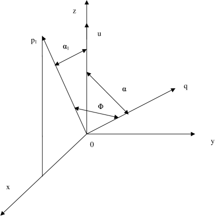
Figure 6: The coordinate system in “q”-space under fixing value of vector ${\bf p}_{1}$.

Then the coordinates of vectors ${\bf q}$ and ${\bf p}_{1}$ are equal to ${\bf q}=(|{\bf q}|,\alpha,\psi),\,{\bf p}_{1}=(|{\bf p}_{1}|,{\alpha}_{1},0)$. By $\Phi$ we denote the angle between ${\bf p}_{1}$ and ${\bf q}$: $({\bf p}_{1}\cdot{\bf q})=|{\bf p}_{1}||{\bf q}|\cos\Phi$. The angle $\Phi$ can be expressed as

$$\cos\Phi=\sin\alpha\sin{\alpha}_{1}\cos\psi+\cos\alpha\cos{\alpha}_{1},$$ (8.2)

and the integration measure is $d{\bf q}={\bf q}^{2}d|{\bf q}|d\psi\sin\alpha\,d\alpha.$ The integral over polar angle $\alpha$ by virtue of $\delta$-function determines the value $\alpha=\pi/2$ in the integrand (8.1). Futhermore for integration over momentum ${\bf p}_{1}$ it is convenient going to coordinate system in which axis 0Z is aligned with velocity $\check{\bf v}$ of energetic parton, as it was depicted in Fig.7.

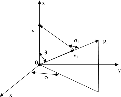
Figure 7: The coordinate system in “${\bf p}_{1}$”-space.

Then the coordinate of vector ${\bf p}_{1}$ is equal to ${\bf p}_{1}=(|{\bf p}_{1}|,\vartheta,\phi)$. The following relations

$$|{\bf u}|\cos{\alpha}_{1}=|\check{\bf v}|\cos\vartheta-|{\bf v}_{\bf p}^{l}|,$$

$$|{\bf u}|\sin{\alpha}_{1}=|\check{\bf v}|\sin\vartheta\hskip 39.83368pt$$

are true. The integration measure with respect to “${\bf p}_{1}\!$”-space is $d{\bf p}_{1}={\bf p}_{1}^{2}d|{\bf q}|d\phi\sin\vartheta d\vartheta.$ Taking into account above-mentioned, the expression (8.1) can be presented in the form

$$\left(\!-\frac{dE^{(1)l}}{dx}\right)^{\!{\rm sp}}\!\simeq\frac{2\pi}{|\check{\bf v}|}\left(\frac{N_{c}\alpha_{s}}{2{\pi}^{2}}\right)^{2}\!\int\limits_{0}^{\infty}\!d|{\bf p}_{1}|\,{\bf p}_{1}^{2}\,\omega_{{\bf p}_{1}}^{l}N_{{\bf p}_{1}}^{l}\!\left(\frac{{\rm Z}_{l}({\bf p}_{1})}{2\omega_{{\bf p}_{1}}^{l}}\right)^{\!2}\!\left(\frac{p_{1}^{2}}{{\bf p}^{2}_{1}}\right)^{\!2}$$ (8.3)

$$\times\int\limits_{0}^{2\pi}\!d\phi\!\int\limits_{-1}^{1}\!d\cos\vartheta\frac{1}{|{\bf u}|}\!\int\limits_{0}^{|{\bf q}^{\ast}|}\!d|{\bf q}||{\bf q}|\!\int\limits_{-1}^{1}\!d\!\cos\alpha\,\delta(\cos\alpha)\left|{\rm T}^{\perp}(\check{\bf v}|\,{\bf p},{\bf p}_{1})\right|^{2}.$$

Running ahead we note that angle singularity mentioned in closing previous Section is connected with singularity with respect to angle variable $\alpha_{1}$. This singularity has dynamical origin, since it connected with medium induced three-wave vertex $\delta\Gamma^{(3)}$. The consequence of this angle singularity will be appearing selected directions in initial isotropic hot gluon plasma. It is the directions of primary rescattering of plasmons by hard parton, or directions over which a main energy loss of parton arise. By virtue of this fact, the basic characteristic of interaction process of a high energy incident parton with a hot QCD medium, in addition to integral energy loss (8.3), is the angular dependence of the energy loss

$$\left(\!-\frac{dE^{(1)l}}{d\vartheta dx}\right)^{\!{\rm sp}}$$

with respect to velocity direction $\check{\bf v}$. We turn to derivation and analysis of this function.

Using an explicit expression for HTL-correction $\delta\Gamma^{00j}$ (Eq. (3.30) in work Frenkel and Taylor [2]), the initial scattering amplitude ${\rm T}^{\perp}$ can be presented in an analytic form

$${\rm T}^{\perp}(\check{\bf v}|\,{\bf p},{\bf p}_{1})=\frac{({\bf v}\cdot({\bf n}\times{\bf q}))}{{\bf q}^{2}{\bf n}^{2}}\,\biggl{\{}\Bigl{[}({\bf p}\cdot{\bf q})\omega_{1}-\omega({\bf p}_{1}\cdot{\bf q})\Bigr{]}\,\delta\Gamma^{000}(p,-p_{1},-q)$$ (8.4)

$$+\,{\bf q}^{2}\Pi^{00}(q)+\Bigl{[}2{\bf n}^{2}+({\bf p}\cdot{\bf q}){\bf p}^{2}-({\bf p}_{1}\cdot{\bf q}){\bf p}^{2}_{1}\Bigr{]}\biggl{\}}\!\,^{\ast}{\!\Delta}^{\!t}(q)\Bigl{|}_{\rm on-shell},$$

where ${\bf n}=({\bf p}\times{\bf p}_{1})$, and vertex correction $\delta\Gamma^{000}$ is

$$\delta\Gamma^{000}(p,-p_{1},-q)=-m_{D}^{2}\left\{\omega_{1}{\rm M}(p_{1},q)-\omega{\rm M}(p,q)+\frac{i\pi q_{0}}{2\sqrt{-\Delta}}\,\theta(-\Delta)\right\},$$ (8.5)

with

$${\rm M}(p,q)=\displaystyle\frac{1}{2\sqrt{-\Delta(p,q)}}\ln\!\left(\displaystyle\frac{p\cdot q+\sqrt{-\Delta(p,q)}}{p\cdot q-\sqrt{-\Delta(p,q)}}\right),\;\;\Delta(p,q)\equiv p^{2}q^{2}-(p\cdot q)^{2}|_{\rm on-shell}<0,$$

and finally gluon self-energy $\Pi^{00}$ is

$$\Pi^{00}(q)=m_{D}^{2}\bigg{[}1-F\bigg{(}\frac{q_{0}}{|{\bf q}|}\bigg{)}\bigg{]}\;,\;F(x)\equiv\frac{x}{2}\bigg{[}\ln\bigg{|}\frac{1+x}{1-x}\bigg{|}-i\pi\theta(1-|x|)\bigg{]},$$ (8.6)

where $q_{0}\equiv({\bf v}\cdot{\bf q})$. In approximation of a small momentum transfer $|{\bf q}|\leq|{\bf q}^{\ast}|$ and large phase velocity of plasmons $\omega^{l}_{{\bf p}_{1}}/|{\bf p}_{1}|\gg 1$, the expressions in square braces in Eq. (8.4) can be set equal

$$({\bf p}\cdot{\bf q})\omega_{{\bf p}_{1}}^{l}-\omega_{\bf p}^{l}({\bf p}_{1}\cdot{\bf q})\simeq{\bf q}^{2}\omega_{{\bf p}_{1}}^{l},\qquad 2{\bf n}^{2}+({\bf p}\cdot{\bf q}){\bf p}^{2}-({\bf p}_{1}\cdot{\bf q}){\bf p}^{2}_{1}\simeq 3{\bf q}^{2}{\bf p}_{1}^{2},$$

and the medium-induced vertex $\delta\Gamma^{000}$ reads

$$\omega_{{\bf p}_{1}}^{l}\delta\Gamma^{000}(p,-p_{1},-q)\simeq m_{D}^{2}\left[1-\frac{q_{0}}{2|{\bf q}|}\ln\left|\frac{|{\bf q}|+q_{0}}{|{\bf q}|-q_{0}}\right|-i\pi\,\frac{q_{0}}{2|{\bf q}|}\right].$$ (8.7)

As we see from Eq. (8.4), in this approximation the exact cancellation of the contribution with $\delta\Gamma^{000}$ with gluon self-energy (8.6) is arisen, and therefore expression for scattering amplitude ${\rm T}^{\perp}$ has a simple form

$${\rm T}^{\perp}(\check{\bf v}|\,{\bf p}_{1},{\bf q})\simeq 3{\bf p}_{1}^{2}\,{}^{\ast}{\!\Delta}^{\!t}(q)\,\frac{\check{\bf v}\cdot(({\bf q}\times{\bf p}_{1})\times{\bf q})}{({\bf q}\times{\bf p}_{1})^{2}}.$$ (8.8)

We approximate the transverse scalar propagator $\!\,{}^{\ast}{\!\Delta}^{\!t}(q)$ by its infrared limit as $q_{0}\ll|{\bf q}|\rightarrow 0$ over surface $(\check{\bf v}\cdot{\bf q})=({\bf v}_{{\bf p}_{1}}^{l}\cdot{\bf q})$, namely

$$\!\,{}^{\ast}{\!\Delta}^{\!t}(q)\simeq\frac{1}{({\bf q}^{2}+{\mu}^{2})-\displaystyle\frac{i\pi}{2}m_{D}^{2}|{\bf v}_{{\bf p}_{1}}^{l}\!|\cos\Phi},$$ (8.9)

where the angle $\Phi$ is derived by relation (8.2). Here, we introduce the magnetic “mass” $\mu$ to screen the infrared singularity.

After integration over angle $\alpha$ in Eq. (8.3) the expression for amplitude (8.8) reads

$${\rm T}^{\perp}(\check{\bf v}|\,{\bf p}_{1},{\bf q})\simeq 3{\bf p}_{1}^{2}\,{}^{\ast}{\!\Delta}^{\!t}(q)\,\frac{|{\bf u}|\cos{\alpha}_{1}}{1-{\sin}^{2}\alpha_{1}{\cos}^{2}\psi},$$ (8.10)

and in the propagator (8.9) it is necessary to set $\cos\Phi=\sin{\alpha}_{1}\cos\psi$. The integrand for loss (8.3) represents a very complicated function of angle $\psi$. However, here, one can use the fact that propagator (8.9) represents a “smooth” function of angle variables with respect to the function going from vertex part in Eq. (8.10). The last one has a singularity with respect to variable $\cos{\alpha}_{1}$. For this reason within accepted computing accuracy we can factor out the function $|\!\,^{\ast}{\!\Delta}^{\!t}(q)|^{2}$ from the integral with respect to angle $\psi$, replacing it to average over $\psi$ on interval $(0,2\pi)$

$$|\!\,^{\ast}{\!\Delta}^{\!t}(q)|^{2}\rightarrow\overline{|\!\,^{\ast}{\!\Delta}^{\!t}(q)|^{2}}=\frac{1}{2\pi}\!\int\limits_{0}^{2\pi}\!|\!\,^{\ast}{\!\Delta}^{\!t}(q)|^{2}d\psi=\frac{1}{({\bf q}^{2}+{\mu}^{2})\sqrt{({\bf q}^{2}+{\mu}^{2})+\chi_{{\bf p}_{1}}^{2}{\sin}^{2}\alpha_{1}}}\,,$$ (8.11)

where $\chi_{{\bf p}_{1}}\equiv(\pi/2)m_{D}|{\bf v}_{{\bf p}_{1}}^{l}\!|$. The remainning integral over $d\psi$ in a general expression (8.3) is simple calculated and by virtue of (8.10) equals

$${\cos}^{2}\alpha_{1}\!\int\limits_{0}^{2\pi}\!\frac{d\psi}{(1-{\sin}^{2}\alpha_{1}{\cos}^{2}\psi)^{2}}=\pi\,\frac{1+{\cos}^{2}\alpha_{1}}{|\cos\alpha_{1}|}.$$

We remind that angle $\alpha_{1}$ is connected with angle $\vartheta$ by means of equality $|{\bf u}|\cos\alpha_{1}=|\check{\bf v}|\cos\vartheta-|{\bf v}_{{\bf p}_{1}}^{l}\!|$, and therefore the last relation has singularity in point $|{\bf v}_{{\bf p}_{1}}^{l}\!|=|\check{\bf v}|\cos\vartheta$. This, in particular, enables us to approximate the relative velocity

$$|{\bf u}|^{2}=\check{\bf v}^{2}+{\bf v}_{{\bf p}_{1}}^{l\,2}-2|\check{\bf v}||{\bf v}_{{\bf p}_{1}}^{l}\!|\cos\vartheta\simeq\check{\bf v}^{2}{\sin}^{2}\vartheta.$$

We set the plasmon number density $N_{{\bf p}_{1}}^{l}$ by step function

$$N_{{\bf p}_{1}}^{l}=\left\{\begin{array}[]{ll}\displaystyle\frac{1}{g^{\rho}}N_{0},&|{\bf p}_{1}|\leq|{\bf p}_{1}|_{\rm max}\\ 0,&|{\bf p}_{1}|>|{\bf p}_{1}|_{\rm max},\end{array}\right.$$

where $N_{0}$ is a certain constant independing of coupling $g$, parameter $1\leq\rho\leq 2$. The parameter $\rho$, as it have been discussed in Section 5, determines a level of soft plasma excitations (or value of plasmon occupation number). In deciding on value $|{\bf p}_{1}|_{\rm max}$ we can guide by the next circumstance. The leading order dispersion equation (I.2.1) defines a spectrum of longitudinal oscillations for the entire $(\omega,|{\bf p}|)$-plane. However it was shown (for QCD case in Refs. [47] and for SQED case in Ref. [49]), that by virtue of specific behaviour of longitudinal oscillation spectrum near light-cone $\omega=|{\bf p}|$, consideration next-to-leading terms in the dispersion equation leads to important qualitative change. There is only a finite range of $|{\bf p}|$ in which longitudinal plasmons can exist. Therefore as $|{\bf p}_{1}|_{\rm max}$ one can choose a value of plasmon momentum such that modified dispersion curve hit the light-cone. For pure gluon plasma we have [49]

$$|{\bf p}_{1}|_{\rm max}^{2}=3\,\omega_{\rm pl}^{2}\left[\,\ln\Biggl{(}\frac{2\sqrt{6}}{g\sqrt{N_{c}}}\Biggr{)}+\frac{1}{2}-\gamma_{E}+\frac{\zeta^{\prime}(2)}{\zeta(2)}\,\right],$$ (8.12)

where $\gamma_{E}$ is an Euler’s constant and $\zeta$ is the Riemann zeta function.

The chosen approximation for plasmon number density is very crude, and we pursue only an aim of obtaining explicit analytical expression for energy loss. The dependence $N_{\bf p}^{l}$ on ${\bf p}$ is determined by solution of kinetic equation (2.1), where the right-hand side represents a sum of collision terms (2.2) – (2.4), (I.2.3) – (I.2.5) etc. (see, e.g. for ordinary plasma Refs. [43]). In this case as an alternative value of $|{\bf p}_{1}|_{\rm max}$, Eq. (8.12), one can consider

$$|{\bf p}_{1}|_{\rm max}^{2}\simeq\biggl{(}\int\!{\bf p}_{1}^{2}N_{{\bf p}_{1}}^{l}\frac{d{\bf p}_{1}}{(2\pi)^{3}}\biggr{)}\!\biggm{/}\!\biggl{(}\int\!N_{{\bf p}_{1}}^{l}\frac{d{\bf p}_{1}}{(2\pi)^{3}}\biggr{)},$$

i.e. $|{\bf p}_{1}|_{\rm max}$ will be dependent on temperature by very nontrivial manner.

With regard to all above-mentioned approximation and ${\rm Z}^{l}({\bf p}_{1})\stackrel{{\scriptstyle{\bf p}_{1}^{2}\rightarrow 0}}{{\longrightarrow}}1$, we find the next expression for the angular dependence of the energy loss of a hard parton from Eq. (8.3)

$$\left(\!-\frac{dE^{(1)l}}{d\vartheta dx}\right)^{\!{\rm sp}}\simeq\left(\frac{N_{c}\alpha_{s}}{2{\pi}^{2}}\right)^{\!2}\frac{9\pi^{3}}{g^{\rho}}\,\omega_{\rm pl}^{3}N_{0}|\check{\bf v}|\,{\sin}^{3}\vartheta\!\int\limits_{0}^{|{\bf p}_{1}\!|_{\rm max}}\!\frac{d|{\bf p}_{1}|}{\left||{\bf v}_{{\bf p}_{1}}^{l}|-|\check{\bf v}|\cos\vartheta\right|}\!\int\limits_{0}^{|{\bf q}^{\ast}|}\!d|{\bf q}|\,|{\bf q}|\,\overline{|\,\!\,^{\ast}{\!\Delta}^{\!t}(q)|^{2}}.$$ (8.13)

Using expression for mean value of scalar propagator (8.11), the integral over $d|{\bf q}|$ is easily calculated and in two limiting cases it equals

$$\int\limits_{0}^{|{\bf q}^{\ast}|}\!d|{\bf q}|\,|{\bf q}|\,\overline{|\,\!\,^{\ast}{\!\Delta}^{\!t}(q)|^{2}}\simeq\frac{1}{2}\!\int\limits_{1/|{\bf q}^{\ast}|^{2}}^{1/{\mu}^{2}}\!\frac{dz}{\sqrt{1+z^{2}\chi_{{\bf p}_{1}}^{2}}}=\left\{\begin{array}[]{ll}\displaystyle\frac{1}{2\chi_{{\bf p}_{1}}}\ln\!\left(\frac{|{\bf q}^{\ast}|^{2}}{\mu^{2}}\right)&,\,\mu^{2}\ll\chi_{{\bf p}_{1}}\\ \displaystyle\frac{1}{2\mu^{2}}&,\,\mu^{2}\gg\chi_{{\bf p}_{1}}.\end{array}\right.$$

By using this fact, we can approximate this integral by the following expression

$$\int\limits_{0}^{|{\bf q}^{\ast}|}\!d|{\bf q}|\,|{\bf q}|\,\overline{|\,\!\,^{\ast}{\!\Delta}^{\!t}(q)|^{2}}\simeq\theta(\chi_{{\bf p}_{1}}-\mu^{2})\,\frac{1}{2\chi_{{\bf p}_{1}}}\ln\!\left(\frac{|{\bf q}^{\ast}|^{2}}{\mu^{2}}\right)+\theta(\mu^{2}-\chi_{{\bf p}_{1}})\,\frac{1}{2\mu^{2}}.$$ (8.14)

Here, on the right-hand side we leave the terms which are more singular over $\mu^{2}$. Magnetic screening mass in the approximation (8.14) carries out separation of plasmons over group velocity ${\bf v}_{{\bf p}_{1}}^{l}$ on “fast” ($\chi_{{\bf p}_{1}}\geq\mu^{2}$) and “slow” ones ($\chi_{{\bf p}_{1}}\leq\mu^{2}$).

We going in Eq. (8.13) from integrating over $|{\bf p}_{1}|$ to integrating over $|{\bf v}_{{\bf p}_{1}}^{l}\!|$, setting for small $|{\bf p}_{1}|$: $d|{\bf p}_{1}|\simeq(5/3)\omega_{\rm pl}d|{\bf v}_{{\bf p}_{1}}^{l}\!|\equiv(5/3)\omega_{\rm pl}dv_{1}$. Then with regard to (8.14) we will have instead of (8.13)

$$\left(\!-\frac{dE^{(1)l}}{d\vartheta dx}\right)^{\!{\rm sp}}\simeq\left(\frac{N_{c}\alpha_{s}}{2{\pi}^{2}}\right)^{2}G^{2}|\check{\bf v}|\,{\sin}^{3}\vartheta$$ (8.15)

$$\times\left\{\ln\!\left(\frac{|{\bf q}^{\ast}|^{2}}{\mu^{2}}\right)\!\!\int\limits_{0}^{v_{1{\rm max}}}\!\theta\Bigl{(}v_{1}-\frac{2\mu^{2}}{\pi m_{D}^{2}}\Bigr{)}\,\frac{dv_{1}}{v_{1}\left|v_{1}-|\check{\bf v}|\cos\vartheta\right|}+\frac{\pi m_{D}^{2}}{2\mu^{2}}\!\int\limits_{0}^{v_{1{\rm max}}}\!\theta\Bigl{(}\frac{2\mu^{2}}{\pi m_{D}^{2}}-v_{1}\Bigr{)}\,\frac{dv_{1}}{\left|v_{1}-|\check{\bf v}|\cos\vartheta\right|}\right\},$$

$$\,G^{2}\equiv\frac{5\pi^{2}}{3}\,\frac{1}{g^{\rho}}\,m_{D}^{2}N_{0},\quad v_{1\,{\rm max}}=\frac{3|{\bf p}_{1}|_{\rm max}}{5\omega_{\rm pl}}.\hskip 85.35826pt$$

The integrals on the right-hand side of Eq. (8.15) are well defined in regions $|\check{\bf v}|\cos\vartheta<0$ and $|\check{\bf v}|\cos\vartheta>v_{1\,{\rm max}}$. In the region $0<|\check{\bf v}|\cos\vartheta<v_{1\,{\rm max}}$ these integrals contain non-integrating singularity, and here, the procedure of their extension to finite value is required.

Now we introduce the notation for integrals entering into the right-hand side of Eq. (8.15)

$$V(z|\,a,b)\equiv\int\limits_{a}^{b}\!\frac{dy}{|y-z|},\;0\leq a<b<1\,;\quad W(z|\,a,b)\equiv\int\limits_{a}^{b}\!\frac{dy}{y|y-z|},\;0<a<b<1,$$

$$|z|\leq 1.$$

We extend the functions $V(z|\,a,b)$ and $W(z|\,a,b)$ based on requirement of continuous of total loss $(dE^{(1)l}/dx)^{\rm sp}$ as velocity function of energetic parton in the neighborhood of value $|\check{\bf v}|=v_{1\,{\rm max}}$. The result of extension is

$$V(z|\,a,b)=\theta(a-z)\,\ln\!\left(\frac{b-z}{a-z}\right)+\theta(z-a)\theta(b-z)\,\ln\!\left(\frac{1}{(z-a)(b-z)}\right)$$

$$+\,\theta(z-b)\,\ln\!\left(\frac{z-a}{z-b}\right),$$ (8.16)

$$W(z|\,a,b)=\theta(a-z)\,\frac{1}{z}\,\ln\!\left(\frac{a(b-z)}{b(a-z)}\right)+\theta(z-a)\theta(b-z)\,\frac{1}{z}\,\ln\!\left(\frac{z-(z-a)^{2}(b-z)}{a(z-a)(b-z)}\right)$$

$$+\,\theta(z-b)\,\frac{1}{z}\,\ln\left(\frac{b(z-a)}{a(z-b)}\right).$$ (8.17)

These extended expressions are logarithmic diverge on the endpoint of integration interval.

The existence of singularities over variable $|\check{\bf v}|\cos\vartheta$ leads to that the angle distribution of energy loss $(-dE^{(1)l}/d\vartheta dx)^{\rm sp}$ has sharp peak in definite directions with respect to vector of velocity $\check{\bf v}$, that as was mentioned above, it can be considered as more probably directions of plasmons reradiation, after their scattering off energetic parton. If reradiated plasmons are sufficiently energetic, i.e. $|{\bf v}_{{\bf p}_{1}}^{l}\!|\sim v_{1\,{\rm max}}$ then here, one can tell about formation of plasmon jets along these directions, which after hadronization can be manifested in the typical hadron distribution.

Let us calculate the contribution to $(-dE^{(1)l}/d\vartheta dx)^{\rm sp}$ of the region of fast plasmons $v_{1\,{\rm max}}-\delta<|{\bf v}_{{\bf p}_{1}}^{l}\!|<v_{1\,{\rm max}}$, where parameter $\delta$ is defined in the interval $0<\delta<v_{1\,{\rm max}}-2\mu^{2}/\pi m_{D}^{2}$. From the general expression (8.15) in this case we have

$$\left(\!-\frac{dE^{(1)l}}{d\vartheta dx}\right)^{\!{\rm sp}}_{\!{\rm fast}}\!\simeq\left(\frac{N_{c}\alpha_{s}}{2{\pi}^{2}}\right)^{2}G^{2}|\check{\bf v}|\,{\sin}^{3}\vartheta\ln\!\left(\frac{|{\bf q}^{\ast}|^{2}}{\mu^{2}}\right)W(|\check{\bf v}|\cos\vartheta|\,v_{1{\rm max}}-\delta,v_{1{\rm max}}),$$

where the function $W$ is defined by Eq. (8.17). In the Fig. 8 the dependence of this expression from $\cos\vartheta$ for $\delta=0,2$ and 0,05; $|\check{\bf v}|=1$ and choice $v_{1\,{\rm max}}\simeq 3/5$, is given.

Figure 8: The dependence $\left(\!-\frac{dE^{(1)l}}{d\vartheta dx}\right)^{\!{\rm sp}}_{\!{\rm fast}}$ from $\cos\vartheta$ for $\delta=0,2$ (solid) and $\delta=0,05$ (point) under $|\check{\bf v}|=1$.

The typical peculiarity of this dependence is presence of sufficiently sharp boundary over angle $\vartheta$, for which the loss become essential. This boundary is determined by $\cos{\vartheta}_{0}=v_{1{\rm max}}/|\check{\bf v}|$.

The angle distribution of energy loss from whole region of rescattering plasmons $0<|{\bf v}^{l}_{{\bf p}_{1}}\!|<|{\bf v}^{l}_{{\bf p}_{1}}\!|_{\rm max}$, is presented in Fig.9. It is seen that main loss is connected with

Figure 9: The dependence $\left(\!-\frac{dE^{(1)l}}{d\vartheta dx}\right)^{\!{\rm sp}}$ from $\cos\vartheta$ for whole region of rescattering plasmons, $0<|{\bf v}^{l}_{{\bf p}_{1}}\!|<|{\bf v}^{l}_{{\bf p}_{1}}\!|_{\rm max}$ under $|\check{\bf v}|=1$.

creation of “slow” plasmons $|{\bf v}^{l}_{{\bf p}_{1}}\!|\sim 0$ and lie in region $\vartheta\sim\pi/2$.

Now we calculate the total energy loss. Integrating the expression (8.15) over angle $\vartheta$ and using (8.16), (8.17) we will have

$$\left(\!-\frac{dE^{(1)l}}{dx}\right)^{\!{\rm sp}}\!=\;\left(\!-\frac{dE^{(1)l}}{dx}\right)^{\!{\rm sp}}_{\!v_{1}<2\mu^{2}\!/\pi m_{D}^{2}}+\,\;\;\left(\!-\frac{dE^{(1)l}}{dx}\right)^{\!{\rm sp}}_{\!v_{1}>2\mu^{2}\!/\pi m_{D}^{2}}$$

$$\equiv\left(\frac{N_{c}\alpha_{s}}{2{\pi}^{2}}\right)^{\!2}\!\frac{G^{2}}{|\check{\bf v}|^{2}}\,\frac{\pi m_{D}^{2}}{2\mu^{2}}\!\int\limits_{-|\check{\bf v}|}^{|\check{\bf v}|}\!dz\,(|\check{\bf v}|^{2}-z^{2})\,V\Bigl{(}z\Bigm{|}\,0,\frac{2\mu^{2}}{\pi m_{D}^{2}}\Bigr{)}$$ (8.18)

$$+\,\left(\frac{N_{c}\alpha_{s}}{2{\pi}^{2}}\right)^{\!2}\!G^{2}\ln\!\left(\frac{|{\bf q}^{\ast}|^{2}}{\mu^{2}}\right)\!\int\limits_{-|\check{\bf v}|}^{|\check{\bf v}|}\!dz\,(|\check{\bf v}|^{2}-z^{2})\,W\Bigl{(}z\Bigm{|}\,\frac{2\mu^{2}}{\pi m_{D}^{2}},\frac{3}{5}\Bigr{)},$$

where in the last line we set $v_{1\,{\rm max}}=3/5$. Using an explicit expression for function $V$ (Eq. (8.16)), we derive in limit $\mu^{2}\rightarrow 0$ an asymptotic expression for contribution from “slow” plasmons

$$\left(\!-\frac{dE^{(1)l}}{dx}\right)^{\!{\rm sp}}_{\!v_{1}<2\mu^{2}\!/\pi m_{D}^{2}}\simeq\;\left(\frac{N_{c}\alpha_{s}}{2{\pi}^{2}}\right)^{\!2}\!4G^{2}\ln\!\left(\frac{\pi m_{D}^{2}}{2\mu^{2}}\right)\!+{\rm const}+O(\mu^{2})+\ldots\,.$$ (8.19)

Similar calculations result in asymptotic expression for the second contribution on the right-hand side of (8.18)

$$\left(\!-\frac{dE^{(1)l}}{dx}\right)^{\!{\rm sp}}_{\!v_{1}>2\mu^{2}\!/\pi m_{D}^{2}}\simeq\;\left(\frac{N_{c}\alpha_{s}}{2{\pi}^{2}}\right)^{\!2}\!G^{2}\ln\!\left(\frac{|{\bf q}^{\ast}|^{2}}{\mu^{2}}\right)\left\{\frac{3}{2}\,{\ln}^{2}\!\left(\frac{\pi m_{D}^{2}}{2\mu^{2}}\right)+\ln\!|\check{\bf v}|\ln\!\left(\frac{\pi m_{D}^{2}}{2\mu^{2}}\right)\right.$$

$$\left.+\,\ln\left(\frac{|\check{\bf v}|}{v_{1{\rm max}}}\right)\ln\!\left(\frac{v_{1{\rm max}}\pi m_{D}^{2}}{2\mu^{2}}\right)\theta(|\check{\bf v}|-v_{1{\rm max}})+{\rm const}+O(\mu^{2})+\ldots\,\right\}.$$ (8.20)

We see from Eq. (8.19) and (8.20) that a main contribution to energy loss in the limit $\mu^{2}\rightarrow 0$ is connected with a first term in braces on the right-hand side of Eq. (8.20). Thus leading contribution to parton energy loss, caused by spontaneous scattering off plasmons in hot gluon plasma is defined by expression

$$\left(\!-\frac{dE^{(1)l}}{dx}\right)^{\!{\rm sp}}\simeq\frac{5N_{0}N_{c}^{3}}{24\pi^{2}}\,g^{2-\rho}\alpha_{s}^{2}T^{2}\ln\!\left(\frac{|{\bf q}^{\ast}|^{2}}{\mu^{2}}\right){\ln}^{2}\!\left(\frac{\pi m_{D}^{2}}{2\mu^{2}}\right).$$ (8.21)

For highly excited plasma, when $\rho\simeq 2$, suppression in coupling constant of this process of energy loss as compared with polarization loss [17], is not arisen. Moreover here, we have two logarithmic enhacements. The first of them is connected with absence of sreening in scalar propagator $\!\,{}^{\ast}\!\Delta^{\!t}(q)$, that gives a factor $\ln(|{\bf q}^{\ast}|^{2}\!/\mu^{2})$. The second one is associated with singularity of integrand of Eq. (8.3) with respect to angle variable $\alpha_{1}$ in point $\alpha_{1}=\pi/2$. This singularity sets a singular curve $v_{1}-|\check{\bf v}|\cos\vartheta=0$ in variables space $(\vartheta,v_{1})$, whose consequence is appearing of logarithmic singularities with respect to angle $\vartheta$ in points $\vartheta\sim\pi/2$ and $\vartheta\sim\vartheta_{0}=\arccos\,(|\check{\bf v}|/v_{1{\rm max}})$. They lead to a factor ${\ln}^{2}(\pi m_{D}^{2}/2\mu^{2})$ in expession for loss (8.21). It can be assumed that this angle singularity is associated with the massless basic constituents of a hot gluon plasma, i.e. with massless of hard transverse gluons. The inclusion of the asymptotic thermal mass $m_{g,\,\infty}^{2}=g^{2}T^{2}N_{c}/6$ for hard thermal gluons and use of the improved three-gluon HTL amplitude $\!\,{}^{\ast}\Gamma_{\mu\mu_{1}\mu_{2}}(p,-p_{1},-p_{2})$ [48] can removes this type of singularity. This hypothesis requires separate and more careful consideration.

9 Off-diagonal contribution to energy loss

In this Section we briefly analyze on a qualitative level a role of off-diagonal term (7.9) in the process of energy loss of energetic parton. Gailitis and Tsytovich [36] have pointed to the necessity of considering this contribution within usual plasma, and here, we extend the conclusions of this work to non-Abelian case.

Using the explicit expression for effective current $\tilde{J}_{Q\mu}^{(2)ab}(p)$ (7.3) and leaving only longitudinal parts in the propagator and correlation function we lead to the expression (instead of (7.9))

$$\left(\!-\frac{dE^{(1)l}}{dx}\right)^{\!{\rm pol}}\!=\frac{(2\pi)^{3}}{|\check{\bf v}|}\Biggl{(}\frac{N_{c}\alpha_{s}}{2{\pi}^{2}}\Biggr{)}^{\!2}\!\frac{1}{d_{A}N_{c}}\!\int\!dpdp_{1}\,{\omega}^{2}\left(\frac{p^{2}}{{\omega}^{2}{\bf p}^{2}}\right)\!\left(\frac{p^{2}_{1}}{{\omega}^{2}_{1}{\bf p}^{2}_{1}}\right)\frac{1}{{\omega}_{1}^{2}}\langle{\bf E}^{2}_{l}{\rangle}_{p_{1}}$$ (9.1)

$$\times\,{\rm Im}\,(\!\,^{\ast}{\Delta}^{l}(p))\,{\rm Re}\,\Bigl{(}K^{abba\,ii_{1}i_{1}^{\prime}}(\check{\bf v}|\,p,-p_{1},p_{1})p^{i}p_{1}^{i_{1}}p_{1}^{i_{1}^{\prime}}\Bigr{)}\,\delta(\check{v}\cdot p).$$

The explicit form of the coefficient function $K_{\mu\mu_{1}\mu_{2}}^{aa_{1}a_{2}}(\check{\bf v}|\,p,-p_{1},-p_{2})$ in linear approximation in a color charge $Q_{0}^{b}$ of parton is defined by expression (4.8). With the help of (4.8) we obtain the required expression, where

$$K^{abba\,ii_{1}i_{1}^{\prime}}({\check{\bf v}|\,p,-p_{1},p_{1})={\rm Tr}\,(T^{a}T^{a})\Bigl{\{}\stackrel{{\scriptstyle\scriptscriptstyle{\!\!\!\!\!\!\!\!\!\!(1)}}}{{\displaystyle{K}^{ii_{1}i_{1}^{\prime}}}}\!(\check{\bf v}|\,p,-p_{1},p_{1})+\stackrel{{\scriptstyle\scriptscriptstyle{\!\!\!\!\!\!\!\!\!\!(1)}}}{{\displaystyle{K}^{ii_{1}^{\prime}i_{1}}}}}\!(\check{\bf v}|\,p,p_{1},-p_{1})\Bigr{\}}.$$ (9.2)

The special feature of the last expression is the condition that in spite of the fact that every term in braces on the right-hand side of equation (9.2) contains the singularities of the $1/(\check{v}\cdot p),\,^{\ast}\!\tilde{\cal D}_{\mu\mu^{\prime}}(0)$ etc. types, however in a sum they are reduced. Therefore the expression (9.2) is well-definite and equals

$$K^{abba\,ii_{1}i_{1}^{\prime}}({\check{\bf v}}|\,p,-p_{1},p_{1})=N_{c}d_{A}\biggl{\{}\!\,^{\ast}\tilde{\Gamma}^{ii_{1}ji_{1}^{\prime}}(p,p_{1},-p,-p_{1})\,^{\ast}\tilde{\cal D}^{jj^{\prime}}\!(p)\check{v}^{j^{\prime}}$$

$$-\,\check{v}^{i_{1}^{\prime}}\biggl{(}\,\frac{\check{v}^{i}\check{v}^{i_{1}}}{(\check{v}\cdot p_{1})^{2}}+\frac{1}{(\check{v}\cdot p_{1})}\!\,^{\ast}\Gamma^{ii_{1}j}(p,-p_{1},-p+p_{1})\,^{\ast}\tilde{\cal D}^{jj^{\prime}}\!(p-p_{1})\check{v}^{j^{\prime}}$$ (9.3)

$$-\,\frac{1}{(\check{v}\cdot p_{1})}\!\,^{\ast}\Gamma^{ii_{1}j}(p,p_{1},-p-p_{1})\,^{\ast}\tilde{\cal D}^{jj^{\prime}}\!(p+p_{1})\check{v}^{j^{\prime}}\biggr{)}\biggr{\}}.$$

Futhermore we add off-diagonal contribution (9.1) with expression for polarization loss (7.6). After some regrouping of the terms this sum reads

$$\left(\!-\frac{dE^{(0)l}}{dx}\right)^{\!{\rm pol}}+\left(\!-\frac{dE^{(1)l}}{dx}\right)^{\!{\rm pol}}=\Lambda_{1}+\Lambda_{2}.$$

Here, on the right-hand side the function $\Lambda_{1}$ is

$${\Lambda}_{1}=-\frac{1}{|\check{\bf v}|}\Biggl{(}\frac{N_{c}\alpha_{s}}{2{\pi}^{2}}\Biggr{)}\!\int\!dp\,\Biggl{(}\frac{\omega\,p^{2}}{{\bf p}^{2}}\Biggr{)}{\rm Im}\,(\!\,^{\ast}{\!\Delta}^{l}(p))\biggl{\{}1+{\rm Re}\,(\Pi^{(1)l}(p)\!\,^{\ast}\!{\Delta}^{l}(p))\biggr{\}}\delta(\check{v}\cdot p),$$ (9.4)

where

$$\Pi^{(1)l}(p)\equiv-(2\pi)^{3}\!\Biggl{(}\frac{N_{c}\alpha_{s}}{2{\pi}^{2}}\Biggr{)}\!\left(\frac{p^{2}}{{\omega}^{2}{\bf p}^{2}}\right)\!\int\!dp_{1}\!\left(\frac{p^{2}_{1}}{{\omega}^{2}_{1}{\bf p}^{2}_{1}}\right)\frac{1}{{\omega}_{1}^{2}}\langle{\bf E}^{2}_{l}\rangle_{p_{1}}$$ (9.5)

$$\times\Bigl{[}\!\,^{\ast}\tilde{\Gamma}^{ii_{1}jj_{1}}(p,p_{1},-p,-p_{1})p^{i}p_{1}^{i_{1}}p^{j}p_{1}^{j_{1}}\Bigr{]},$$

and the function ${\Lambda}_{2}$ has the form

$${\Lambda}_{2}\equiv-\frac{(2\pi)^{3}}{|\check{\bf v}|}\Biggl{(}\frac{N_{c}\alpha_{s}}{2{\pi}^{2}}\Biggr{)}^{\!2}\!\!\int\!dpdp_{1}\,{\omega}^{2}\!\left(\frac{p^{2}}{{\omega}^{2}{\bf p}^{2}}\right)\!\left(\frac{p^{2}_{1}}{{\omega}^{2}_{1}{\bf p}^{2}_{1}}\right)\frac{1}{{\omega}_{1}^{2}}\langle{\bf E}^{2}_{l}\rangle_{p_{1}}(\check{\bf v}\cdot{\bf p}_{1})$$ (9.6)

$$\times\,{\rm Im}\,(\!\,^{\ast}{\!\Delta}^{l}(p))\,{\rm Re}\,\Biggl{\{}\frac{\check{v}^{i}\check{v}^{i_{1}}}{(\check{v}\cdot p_{1})^{2}}+\frac{1}{(\check{v}\cdot p_{1})}\,^{\ast}\Gamma^{ii_{1}j}(p,-p_{1},-p+p_{1})\,^{\ast}\tilde{\cal D}^{jj^{\prime}}\!(p-p_{1})\check{v}^{j^{\prime}}$$

$$-\,\frac{1}{(\check{v}\cdot p_{1})}\,^{\ast}\Gamma^{ii_{1}j}(p,p_{1},-p-p_{1})\,^{\ast}\tilde{\cal D}^{jj^{\prime}}\,(p+p_{1})\check{v}^{j^{\prime}}\biggr{\}}p^{i}p_{1}^{i_{1}}\delta(\check{v}\cdot p).$$

Let us analyze the expression ${\Lambda}_{1}$. It can be shown that the entering function $\Pi^{(1)l}(p)$ represents the correction to longitudinal part of gluon self-energy in HTL-approximation (i.e. to $\Pi^{l}(p)$) taking into account change of dielectric properties of hot gluon plasma by the action of the processes of nonlinear interaction (longitudinal) plasma excitations among themselves. For low excited state of plasma ($\delta=1/2$ for estimation (7.7)), corresponding to level of thermal fluctuation, correction $\Pi^{(1)l}(p)$ is suppressed by more power of $g$ in comparison with $\Pi^{l}(p)$. In the limiting case of a strong field $(\delta=0)$ the function $\Pi^{(1)l}(p)$ (and also corrections of higher power in $\langle{\bf E}_{l}^{2}\rangle_{p}$) is the same order in $g$ as gluon self-energy in HTL-approximation, and therefore considering influence of nonlinear plasma processes on the energy loss of energetic parton becomes necessary.

One can define an effective scalar propagator $\!\,{}^{\ast}\!\tilde{\Delta}^{l}(p)$, which takes into account additional contributions, considering nonlinear effects of plasmon self-interactions. Here, we have

$$\!\,{}^{\ast}\!\tilde{\Delta}^{\!-1l}(p)\equiv\!\,^{\ast}\!{\Delta}^{\!-1l}(p)-\sum_{n=1}^{\infty}\Pi^{(n)l}(p),$$ (9.7)

where

$$\Pi^{(n)l}(p)\equiv-(2\pi)^{3}\Biggl{(}\frac{N_{c}\alpha_{s}}{2{\pi}^{3}}\Biggr{)}^{\!n}\!\left(\frac{p^{2}}{{\omega}^{2}{\bf p}^{2}}\right)\!\int\!\prod_{i=1}^{n}dp_{i}\left(\frac{p^{2}_{i}}{{\omega}^{2}_{i}{\bf p}^{2}_{i}}\right)\frac{1}{{\omega}_{i}^{2}}\langle{\bf E}^{2}_{l}\rangle_{p_{i}}$$

$$\times\biggl{[}\,^{\ast}\tilde{\Gamma}^{ii_{1}\ldots i_{n}jj_{1}\ldots j_{n}}(p,p_{1},\ldots,p_{n},-p_{1},\ldots,-p_{n})p^{i}p_{1}^{i_{1}}\ldots p_{n}^{i_{n}}p^{j}p_{1}^{j_{1}}\ldots p_{n}^{j_{n}}\biggr{]}.$$

The algorithm of calculation of the effective subamplitudes $\!\,{}^{\ast}\tilde{\Gamma}^{(n)}$ entering in integrand, was defined in [1]. For low excited state, when $\!\,{}^{\ast}\!{\Delta}^{\!-1l}(p)\gg\Pi^{(1)l}(p)\gg\Pi^{(2)l}(p)\ldots$ from the equation (9.7) to the first order in $\langle{\bf E}^{2}_{l}\rangle_{p_{i}}$ we obtain an approximation

$$\!\,{}^{\ast}\!\tilde{\Delta}^{\!l}(p)\simeq\!\,^{\ast}\!{\Delta}^{\!l}(p)+\!\,^{\ast}\!{\Delta}^{\!l}(p)\,\Pi^{(1)l}(p)\,^{\ast}\!{\Delta}^{\!l}(p),$$

whose imaginary part is equal to

$${\rm Im}\,(\!\,^{\ast}\!\tilde{\Delta}^{\!l}(p))\simeq{\rm Im}\,(\!\,^{\ast}\!{\Delta}^{\!l}(p))\biggl{\{}1+{\rm Re}\,(\Pi^{(1)l}(p)\!\,^{\ast}\!{\Delta}^{l}(p))\biggr{\}}+{\rm Re}\,(\!\,^{\ast}\!{\Delta}^{\!l}(p)){\rm Im}\,(\Pi^{(1)l}(p)\!\,^{\ast}\!{\Delta}^{l}(p)),$$ (9.8)

correspondingly. Here, the first term on the right-hand side is precisely coincident with appropriate function in integrand of (9.4). If the second term is absent on the right-hand side of Eq. (9.8), than the contribution $\Lambda_{1}$ to the energy loss can be interpretated as polarization loss with regard to change of dielectric property of medium induced by plasmon self-nteraction. This can be effective present as a replacement of the HTL resummed longitudinal propagator, entering into expression for polarization loss (7.6) by an effective one

$${}^{\ast}\!{\Delta}^{\!l}(p)\rightarrow\,^{\ast}\tilde{\!\Delta}^{\!l}(p).$$

However the existence of the second term on the right-hand side of Eq. (9.8) gives no way completely restricted ourselves by such simple transition. The physical meaning of this fact is not clear.

Let us analyzed the contribution $\Lambda_{2}$ (Eq. (9.6)). This contribution (as previous one) is not equil to zero only for plasma excitations lying off mass-shell. From the expression for basic diagonal contribution to energy loss (7.11), (7.12) we see that it contains the singularities off-plasmon shell in the forms $1/(\check{v}\cdot p_{1})^{2}$ and $1/(\check{v}\cdot p_{1})$, when frequency and momentum of plasma excitations approach to ”Cherenkov cone”

$$(\check{v}\cdot p_{1})\rightarrow 0.$$

The existence of these singularities causes the large rotation velocity of color vector $Q^{a}$ of energetic parton in random plasma field. However these singularities are exactly compensated by analogous ones in expressions for energy loss $\Lambda_{2}$, Eq. (9.6). It is not difficult to check this by correlating the expressions (7.11) and (9.6). Thus the complete sum of all contributions to energy loss of energetic parton for scattering off plasma excitations lying off-plasmon shell is a finite value, but as supposed it is sufficiently small in comparison with energy loss for scattering off plasma excitations lying on-plasmon shell to neglect it.

10 The Fokker-Planck equation for beam of energetic partons

The goal of this Section is a derivation of the Fokker-Planck equation, describing an evolution of a distribution function $f({\bf k},x,Q)$ for a beam of energetic color partons due to the processes of energy loss and diffusion in momentum space for scattering off soft longitudinal plasma excitations. Let us supposed that particles number density is so small that one can neglect by partons interaction in beam among themselves. One of the consequences of derivation of this equation having relevance to the subject of our study will be obtaining more complete expression for energy loss and also a possible gain of energy of isolated energetic parton of beam which follows from well-known connection of the drag coefficient ${\rm A}^{i}({\bf k})$ with expression for energy loss $dE/dx$ [37], [38].

First of all we consider a more general problem for initial formulation, which in principle gives a possibility to consider a diffusion of beam of energetic color particles in an effective color space on an equal footing with diffusion in momentum space. We assume that a time-space dependent external color current $j_{\mu}^{{\rm ext}\,a}(x)$ starts acting on the system. In this case the soft-gauge field develops an expectation value $\langle A_{\mu}^{a}(x)\rangle\equiv{\cal A}_{\mu}^{a}(x)\neq 0$, and the number density of the plasmons $N_{\bf p}^{lab}$ acquires a nondiagonal color structure. The equation describing the time-space evolution of the distribution function $f({\bf k},x,Q)$ in first approximation in a number of emitted and absorbed plasmons reads

$$\left(\frac{\partial}{\partial t}+\check{\bf v}\cdot\frac{\partial}{\partial{\bf x}}+gQ^{a}\biggl{(}{\bf{\cal E}}^{a}(x)+(\check{\bf v}\times{\bf{\cal B}}^{a}(x))\biggr{)}\cdot\frac{\partial}{\partial{\bf k}}\right)\!f({\bf k},x,Q)$$

$$+\,gf^{abc}\check{v}^{\mu}{\cal A}_{\mu}^{a}(x)\frac{\partial}{\partial Q^{b}}(Q^{c}f({\bf k},x,Q))$$ (10.1)

$$=-\,\frac{1}{2}\!\int\!\frac{d{\bf p}}{(2\pi)^{3}}\frac{d{{\bf p}_{1}}}{(2\pi)^{3}}\,{\it w}_{2}^{\{a^{\prime}\},\{a\}}(\check{\bf v}({\bf k})|\,{\bf p},{\bf p}_{1})$$

$$\times\Bigl{\{}N_{\bf p}^{l\,a^{\prime}a}(N_{{\bf p}_{1}}^{l}+1)^{a_{1}a_{1}^{\prime}}f({\bf k},x,Q)-(N_{\bf p}^{l}+1)^{aa^{\prime}}N_{{\bf p}_{1}}^{la_{1}^{\prime}a_{1}}f({\bf k}+{\bf q},x,Q)\Bigr{\}}$$

$$-\,\frac{1}{2}\!\int\!\frac{d{\bf p}}{(2\pi)^{3}}\frac{d{{\bf p}_{1}}}{(2\pi)^{3}}\,{\it w}_{2}^{\{a\},\{a^{\prime}\}}(\check{\bf v}({\bf k})|\,{\bf p}_{1},{\bf p})$$

$$\times\Bigl{\{}N_{{\bf p}_{1}}^{l\,aa^{\prime}}(N_{\bf p}^{l}+1)^{a_{1}^{\prime}a_{1}}f({\bf k},x,Q)-(N_{{\bf p}_{1}}^{l}+1)^{a^{\prime}a}N_{\bf p}^{la_{1}a_{1}^{\prime}}f({\bf k}-{\bf q},x,Q)\Bigr{\}}.$$

Here, we use a multiindex notation $\{a\}=(a,a_{1})$. In deriving collision integrals on the right-hand side of Eq. (10.1) we take into account a property of scattering probability relative to permutation of the external soft momenta ${\bf p}$ and ${\bf p}_{1}$:

$${\it w}_{2}^{\{a^{\prime}\},\{a\}}(\check{\bf v}({\bf k})|\,{\bf p},{\bf p}_{1})={\it w}_{2}^{\{a\},\{a^{\prime}\}}(\check{\bf v}({\bf k}+{\bf q})|\,{\bf p}_{1},{\bf p}).$$ (10.2)

This property of the scattering probability is a generalization of the property (7.14), since the last one is valid only in the framework of HTL-approximation and for condition $|{\bf q}|\ll|{\bf k}|$. The equality (10.2) is a consequence of detailed balancing principle and therefore is exact. The existence of two collision terms on the right-hand side of Eq. (10.1) takes into account two possible processes of exchange of the beam state of energetic color particles.

In the general case the scattering probability in integrand on the right-hand side of Eq. (10.1) also depends on a color vector $Q=(Q^{b})$. Suppose that this dependence is analytic, i.e. the function ${\it w}_{2}^{\{a^{\prime}\};\{a\}}$ can be represented as an expansion in powers of $Q$ and a first term in this expansion can be written in the form

$${\it w}_{2}^{\{a^{\prime}\},\{a\}}(\check{\bf v}({\bf k})|\,{\bf p},{\bf p}_{1})=\Bigl{(}T^{aa_{1}b}(\check{\bf v}({\bf k})|\,{\bf p},-{\bf p}_{1})Q^{b}\Bigr{)}\Bigl{(}T^{\ast\,a^{\prime}a_{1}^{\prime}b^{\prime}}(\check{\bf v}({\bf k})|\,{\bf p},-{\bf p}_{1})Q^{b^{\prime}}\Bigr{)}$$

$$\times 2\pi\,\delta(E_{\bf k}-E_{{\bf k}+{\bf q}}+\omega_{\bf p}^{l}-\omega_{{\bf p}_{1}}^{l}).$$ (10.3)

Here, $E_{\bf k}$ is energy of hard parton and $T^{aa_{1}b}(\check{\bf v}({\bf k})|\,{\bf p},-{\bf p}_{1})=-if^{aa_{1}b}T(\check{\bf v}({\bf k})|\,{\bf p},-{\bf p}_{1})$ is interaction matrix element. The scalar function $T(\check{\bf v}({\bf k})|\,{\bf p},-{\bf p}_{1})$ is reduced to the function (3.18) in HTL-approximation and small momentum transfers.

Furthermore we restricted our consideration to study of the scattering process of a bundle hard partons off colorless part of soft-gluon excitations, i.e. set on the right-hand side of Eq. (10.1) $N_{\bf p}^{laa^{\prime}}=\delta^{aa^{\prime}}N_{\bf p}^{l}$. If one neglect by influence of a mean field (setting it a small), then kinetic equation (10.1) can be written as equation for momentum of zeroth order in color charge of distribution function

$$f({\bf k},x)=\int\!dQf({\bf k},x,Q).$$

With regard to a structure of scattering probability (10.3), after some algebraic transformation and regrouping the terms, initial equation (10.1) can be introduced in the form more convenient for subsequent study

$$\left(\frac{\partial}{\partial t}+\check{\bf v}\cdot\frac{\partial}{\partial{\bf x}}\right)\!f({\bf k},x)=\left(\frac{\partial f}{\partial t}\right)^{\!{\rm sp}}\!+\left(\frac{\partial f}{\partial t}\right)^{\!{\rm st}}\!,$$ (10.4)

where

$$\left(\frac{\partial f}{\partial t}\right)^{\!{\rm sp}}\!\equiv-\pi\left(\frac{N_{c}\alpha_{s}}{2{\pi}^{2}}\right)^{\!2}\!\left(\frac{C_{2}}{N_{c}}\right)\!\int\!d{\bf p}d{\bf p}_{1}\Bigl{\{}{\it w}_{2}(\check{\bf v}({\bf k})|\,{\bf p},{\bf p}_{1})\Bigl{(}N_{\bf p}^{l}f({\bf k},x)-N_{{\bf p}_{1}}^{l}f({\bf k}+{\bf q},x)\Bigr{)}$$ (10.5)

$$+\,{\it w}_{2}(\check{\bf v}({\bf k})|\,{\bf p}_{1},{\bf p})\Bigl{(}N_{{\bf p}_{1}}^{l}f({\bf k},x)-N_{\bf p}^{l}f({\bf k}-{\bf q},x)\Bigr{)}\Bigr{\}}\delta(E_{\bf k}-E_{{\bf k}+{\bf q}}+\omega_{\bf p}^{l}-\omega_{{\bf p}_{1}}^{l}).$$

is collision term linear in plasmon number density $N_{\bf p}^{l}$ corresponding to spontaneous scattering processes, and

$$\left(\frac{\partial f}{\partial t}\right)^{\!{\rm st}}\!\equiv-\pi\left(\frac{N_{c}\alpha_{s}}{2{\pi}^{2}}\right)^{\!2}\!\left(\frac{C_{2}}{N_{c}}\right)\!\int\!d{\bf p}d{\bf p}_{1}\Bigl{\{}{\it w}_{2}(\check{\bf v}({\bf k})|\,{\bf p},{\bf p}_{1})\,(f({\bf k},x)-f({\bf k}+{\bf q},x))$$ (10.6)

$$+\,{\it w}_{2}(\check{\bf v}({\bf k})|\,{\bf p}_{1},{\bf p})\,(f({\bf k},x)-f({\bf k}-{\bf q},x))\Bigr{\}}N_{\bf p}N_{{\bf p}_{1}}\delta(E_{\bf k}-E_{{\bf k}+{\bf q}}+\omega_{\bf p}^{l}-\omega_{{\bf p}_{1}}^{l})$$

is collision term quadratic in $N_{\bf p}^{l}$ corresponding to stimulated scattering process. Here, a constant $C_{2}\equiv Q^{a}Q^{a}$ is the second order Casimir. We have $C_{2}=C_{A}$ for beam of high energy gluons and $C_{2}=C_{F}$ for quarks. In the scattering probability $w_{2}(\check{\bf v}({\bf k})|\,{\bf p},{\bf p}_{1})\equiv|T(\check{\bf v}({\bf k})|\,{\bf p},-{\bf p}_{1})|^{2}$ we take out a coupling constant and isotopic factors in a coefficient before integral, and the $\delta$-function expressing the energy conservation – in integrand.

Let us consider approximation, when exchange of plasmon momentum in scattering process is much smaller than momentum of energetic parton from beam, that is $|{\bf q}|=|{\bf p}-{\bf p}_{1}|\ll|{\bf k}|$. It enables us to expand the distribution function in powers of $|{\bf q}|$:

$$f({\bf k}\pm{\bf q},x)\simeq f({\bf k},x)\pm\Biggl{(}{\bf q}\cdot\frac{\partial}{\partial{\bf k}}\Biggr{)}f({\bf k},x)+\frac{1}{2!}\,\Biggl{(}{\bf q}\cdot\frac{\partial}{\partial{\bf k}}\Biggr{)}^{\!2}\!f({\bf k},x).$$ (10.7)

The expansion of scattering probability ${\it w}_{2}$ requires a larger accuracy. Let us consider equality ${\it w}_{2}(\check{\bf v}({\bf k})|\,{\bf p}_{1},{\bf p})={\it w}_{2}(\check{\bf v}({\bf k}-{\bf q})|\,{\bf p},{\bf p}_{1})$, which is a consequence of (10.2). We expand the right-hand side in a small parameter $|{\bf q}|/|{\bf k}|$:

$${\it w}_{2}(\check{\bf v}({\bf k})|\,{\bf p}_{1},{\bf p})={\it w}_{2}(\check{\bf v}({\bf k})|\,{\bf p},{\bf p}_{1})-\Biggl{(}{\bf q}\cdot\frac{\partial}{\partial{\bf k}}\Biggr{)}{\it w}_{2}(\check{\bf v}({\bf k})|\,{\bf p},{\bf p}_{1})\,+\ldots\,.$$ (10.8)

The expression ${\it w}_{2}(\check{\bf v}({\bf k})|\,{\bf p},{\bf p}_{1})$ is also required to expand in a small parameter $|{\bf q}|/|{\bf k}|$:

$${\it w}_{2}(\check{\bf v}({\bf k})|\,{\bf p},{\bf p}_{1})={\it w}_{2}^{(0)}(\check{\bf v}({\bf k})|\,{\bf p},{\bf p}_{1})+{\it w}_{2}^{(1)}(\check{\bf v}({\bf k})|\,{\bf p},{\bf p}_{1})+\ldots\,.$$ (10.9)

Substituting the last expansion in the either side of Eq. (10.8), we obtain

$${\it w}_{2}^{(0)}(\check{\bf v}({\bf k})|\,{\bf p},{\bf p}_{1})={\it w}_{2}^{(0)}(\check{\bf v}({\bf k})|\,{\bf p}_{1},{\bf p}),$$ (10.10)

$${\it w}_{2}^{(1)}(\check{\bf v}({\bf k})|\,{\bf p},{\bf p}_{1})={\it w}_{2}^{(1)}(\check{\bf v}({\bf k})|\,{\bf p}_{1},{\bf p})+{\bf q}\cdot\frac{\partial{\it w}_{2}^{(0)}(\check{\bf v}({\bf k})|\,{\bf p},{\bf p}_{1})}{\partial{\bf k}},$$ (10.11)

etc. The principle term of expansion ${\it w}_{2}^{(0)}(\check{\bf v}({\bf k})|{\bf p},{\bf p}_{1})$ represents the scattering probability in quasiclassical approximation with neglecting of recoil of hard parton. Therefore this function is identified with a scattering probability in HTL-approximation (Eqs. (7.15), (7.16)), having the same property of symmetry relative to permutation of soft external momenta (Eq. (7.14)) as (10.10).

At first we consider expansion of collision term defining a process of stimulated scattering. Substituting an expansion (10.7), (10.9) into (10.6) and using the properties (10.10) and (10.11), we obtain that $(\partial f/\partial t)^{\rm st}$ can be introduced in the form of a Fokker-Planck containing the scattering probability in HTL-approximation only

$$\left(\frac{\partial f}{\partial t}\right)^{\!{\rm st}}\simeq\frac{\partial}{\partial k^{i}}\Bigl{(}{\rm A}^{{\rm st},\,i}({\bf k})f\Bigr{)}+\frac{{\partial}^{2}}{\partial k^{i}\partial k^{j}}\Bigl{(}{\rm B}^{{\rm st},\,ij}({\bf k})f\Bigr{)},$$

where the drag and diffusion coefficients respectively are

$${\rm A}^{{\rm st},\,i}({\bf k})=-\pi\left(\frac{N_{c}\alpha_{s}}{2{\pi}^{2}}\right)^{\!2}\!\left(\frac{C_{2}}{N_{c}}\right)\!\int\!q^{i}\biggl{(}{\bf q}\cdot\frac{\partial}{\partial{\bf k}}\,{\it w}_{2}^{(0)}(\check{\bf v}({\bf k})|\,{\bf p},{\bf p}_{1})\biggr{)}N_{\bf p}N_{{\bf p}_{1}}\,\delta(\check{v}\cdot(p-p_{1}))d{\bf p}d{{\bf p}_{1}},$$ (10.12)

$${\rm B}^{{\rm st},\,ij}({\bf k})=\pi\left(\frac{N_{c}\alpha_{s}}{2{\pi}^{2}}\right)^{\!2}\!\left(\frac{C_{2}}{N_{c}}\right)\!\int\!q^{i}q^{j}{\it w}_{2}^{(0)}(\check{\bf v}({\bf k})|\,{\bf p},{\bf p}_{1})N_{\bf p}N_{{\bf p}_{1}}\,\delta(\check{v}\cdot(p-p_{1}))d{\bf p}d{{\bf p}_{1}}.\hskip 45.52458pt$$

In the case of collision term, associated with spontaneous scattering process (Eq. (10.5)) a situation is more complicated. If we perform calculations similar to previous case then we will have

$$\left(\frac{\partial f}{\partial t}\right)^{\!{\rm sp}}\simeq\frac{\partial}{\partial k^{i}}\Bigl{(}{\rm A}^{{\rm sp},\,i}({\bf k})f\Bigr{)}+\frac{{\partial}^{2}}{\partial k^{i}\partial k^{j}}\Bigl{(}{\rm B}^{{\rm sp},\,ij}({\bf k})f\Bigr{)}+\Phi^{(1)}[f],$$

where the drag and diffusion coefficient are

$${\rm A}^{{\rm sp},\,i}({\bf k})=-\pi\left(\frac{N_{c}\alpha_{s}}{2{\pi}^{2}}\right)^{\!2}\!\left(\frac{C_{2}}{N_{c}}\right)\!\int\!q^{i}{\it w}_{2}^{(0)}(\check{\bf v}({\bf k})|\,{\bf p},{\bf p}_{1})(N_{\bf p}^{l}-N_{{\bf p}_{1}}^{l})\,\delta(\check{v}\cdot(p-p_{1}))d{\bf p}d{{\bf p}_{1}}$$

$$-\,\frac{\pi}{2}\left(\frac{N_{c}\alpha_{s}}{2{\pi}^{2}}\right)^{\!2}\!\left(\frac{C_{2}}{N_{c}}\right)\!\int\!q^{i}\biggl{(}{\bf q}\cdot\frac{\partial}{\partial{\bf k}}\,{\it w}_{2}^{(0)}(\check{\bf v}({\bf k})|\,{\bf p},{\bf p}_{1})\biggr{)}(N_{\bf p}^{l}+N_{{\bf p}_{1}}^{l})\,\delta(\check{v}\cdot(p-p_{1}))d{\bf p}d{{\bf p}_{1}},$$ (10.13)

$${\rm B}^{{\rm sp},\,ij}({\bf k})=\frac{\pi}{2}\left(\frac{N_{c}\alpha_{s}}{2{\pi}^{2}}\right)^{\!2}\!\left(\frac{C_{2}}{N_{c}}\right)\!\int\!q^{i}q^{j}{\it w}_{2}^{(0)}(\check{\bf v}({\bf k})|\,{\bf p},{\bf p}_{1})(N_{\bf p}^{l}+N_{{\bf p}_{1}}^{l})\,\delta(\check{v}\cdot(p-p_{1}))d{\bf p}d{{\bf p}_{1}},$$

and the function $\Phi^{(1)}[f]$ is defined by expression

$$\Phi^{(1)}[f]=\frac{\pi}{2}\left(\frac{N_{c}\alpha_{s}}{2{\pi}^{2}}\right)^{\!2}\!\left(\frac{C_{2}}{N_{c}}\right)\!\int\Bigr{\{}{\it w}_{2}^{(1)}(\check{\bf v}({\bf k})|\,{\bf p},{\bf p}_{1})+{\it w}_{2}^{(1)}(\check{\bf v}({\bf k})|\,{\bf p}_{1},{\bf p})\Bigr{\}}(N_{\bf p}^{l}-N_{{\bf p}_{1}}^{l})$$

$$\times\Biggl{(}{\bf q}\cdot\frac{\partial f}{\partial{\bf k}}\Biggr{)}\,\delta(\check{v}\cdot(p-p_{1}))d{\bf p}d{{\bf p}_{1}}.$$

The existence of the last term ${\Phi}^{(1)}[f]$ containing a correction to quasiclassical scattering probability shows that for collision term connected with spontaneous scattering process in limit of a small momentum transfer and accepted calculation accuracy, it is impossible to close on quasiclassical description level. In other words, it is not sufficient to use the properties (10.10) and (10.11) to remove by the next term in expansion of the scattering probability (10.9) considering in fact an effect of quantum response of hard parton.

Nevetheless, having an explicit expression for coefficient functions (10.12), (10.13) we can write the expression for full drag coefficient

$${\rm A}^{i}({\bf k})={\rm A}^{{\rm sp},\,i}({\bf k})+{\rm A}^{{\rm st},\,i}({\bf k})$$

and in so doing to define the energy loss by using relation [37], [38]

$$\frac{dE^{l}}{dx}=-\frac{1}{|{\bf k}|}\,({\bf k}\cdot{\bf A}({\bf k}))\equiv-\frac{1}{|\check{\bf v}|}\,(\check{\bf v}\cdot{\bf A}({\bf k}))$$

$$=-\frac{\pi}{|\check{\bf v}|}\left(\frac{N_{c}\alpha_{s}}{2{\pi}^{2}}\right)^{\!2}\!\left(\frac{C_{2}}{N_{c}}\right)\!\int\!d{\bf p}d{{\bf p}_{1}}{\it w}_{2}^{(0)}(\check{\bf v}({\bf k})|\,{\bf p},{\bf p}_{1})\Bigl{\{}\omega_{\bf p}^{l}N_{{\bf p}_{1}}^{l}+\omega_{{\bf p}_{1}}^{l}N_{\bf p}^{l}\Bigr{\}}\,\delta(\check{v}\cdot(p-p_{1}))$$

$$+\,\frac{\pi}{|\check{\bf v}|}\left(\frac{N_{c}\alpha_{s}}{2{\pi}^{2}}\right)^{\!2}\!\left(\frac{C_{2}}{N_{c}}\right)\!\int\!d{\bf p}d{{\bf p}_{1}}{\it w}_{2}^{(0)}(\check{\bf v}({\bf k})|\,{\bf p},{\bf p}_{1})\Bigl{\{}\omega_{\bf p}^{l}N_{\bf p}^{l}+\omega_{{\bf p}_{1}}^{l}N_{{\bf p}_{1}}\Bigr{\}}\,\delta(\check{v}\cdot(p-p_{1}))$$

$$+\,\frac{\pi}{|\check{\bf v}|}\left(\frac{N_{c}\alpha_{s}}{2{\pi}^{2}}\right)^{\!2}\!\left(\frac{C_{2}}{N_{c}}\right)\!\int\!d{\bf p}d{{\bf p}_{1}}\biggl{(}{\bf q}\cdot\frac{\partial}{\partial{\bf k}}{\it w}_{2}^{(0)}(\check{\bf v}({\bf k})|\,{\bf p},{\bf p}_{1})\biggr{)}$$

$$\times({\omega}_{\bf p}^{l}-{\omega}_{{\bf p}_{1}}^{l})\biggl{\{}\frac{1}{2}(N_{\bf p}^{l}+N_{{\bf p}_{1}}^{l})+N_{\bf p}^{l}N_{{\bf p}_{1}}^{l}\biggr{\}}\,\delta(\check{v}\cdot(p-p_{1})).$$

The first term on the right-hand side exactly reproduces the expression for energy loss (7.13) used in previous Sections for $C_{2}=C_{A}$. The second term defines acceleration obtained by hard color particle for Compton plasmon scattering. As it is seen from this expression in fact it equals the product of total section of this scattering process in HTL approximation by mean energy of longitudinal QGP excitations. It is necessary to take into account this contribution in complete balance of energy loss. The third term is formally suppressed in comparison with the first factor $|{\bf q}|/|{\bf k}|\ll 1$. However it can be expected, that for highly excited state of system, when the plasmon number density is very large, the term in integrand proportional to $N_{\bf p}^{l}N_{{\bf p}_{1}}^{l}$ (stimulated scattering process), can give appreciable contribution to general expression for energy loss. By virtue of the fact that this contribution is indefinit in a general case then here, both drag and acceleration of partons from beam are possible. In particular it depends on concrete form of the plasmon number density $N_{\bf p}^{l}$ as a function of soft momentum ${\bf p}$.

11 Conclusion

In conclusion we would like to dwell on some important moments which remain to be touched upon in this work and on the whole concerned with a mechanism of energy loss studied in previous sections.

In studies of plasmon-hard particle scattering processes and energy losses their related, we consider that a mean-gluon field ${\cal A}_{\mu}^{a}(x)$ in a system equils zero or is so weak that it can be neglected by its influence on dynamics of the processes in QGP. This in particular leads to the fact that we have considered interaction of energetic color particle (or thermal test particle) with colorless part of soft-gluon excitations only. However, opposite case – very strong mean gluon field that is to be necessary account exactly in all orders of perturbation theory, is of great interest. In this case, for example, coefficient functions $K_{\mu\mu_{1}\cdots\mu_{s}}^{aa_{1}\ldots a_{s}}({\bf v}|\,{\bf p},-{\bf p}_{1},\ldots,-{\bf p}_{s})$ under the integral sign of effective currents (7.3) depend by themselves on ${\cal A}_{\mu}^{a}(x)$, i.e. they can contain insertions of an external or self-consisting mean field, in general, of arbitrary order. The interest to such setting up a problem is specified by that it is simpler model for research of jet quenching phenomenon in heavy ion collisions, whereby high-$p_{t}$ partons get depleted through strong (classical) color field.The latter is encountered in the Color Glass Condensate (CGC) [51]. About ten years ago Mc.Lerran and Venugopalan [52] suggest that the prompt phase of heavy ion collisions is CGC, and therefore influence of CGC on energy losses of color partons can be very essential. The example of considering CGC in calculation of energy loss has been given in Introduction. This is a mechanism of synchrotron-like radiation of an ultrarelativistic charge in QCD going through a constant chromomagnetic field, proposed by Shuryak and Zahed [30].

Another important moment that was not touched in this work is concerned with consideration of contributions to energy losses of terms higher in powers of the field in expansion of the effective current (7.2), $s\geq 3$. In principal, in limiting case of a strong random field $|A_{\mu}^{(0)a}(p)|\sim 1/g(gT)^{3}$ (Eq. (7.7)) account must be taken of the whole of series in expansion of the effective current, since formally each term of the series becomes of the same order as a first term $\tilde{J}_{Q\mu}^{(0)}$. A preliminary analysis of contribution to energy loss of higher scattering processes shows that in each subsequent ‘diagonal’ contribution $(-dE^{(n)}/dx)^{\rm sp},\,n\geq 2$, a term having practically the same peculiarity as $(-dE^{(1)}/dx)^{\rm sp}$ can be separated. However, here, we come up against the further problem not allowing directly summarized all relevant terms. These contributions contain the pathological terms generated by product of two $\delta$-functions of $[\delta({\rm Re}\,^{\ast}\!\Delta^{-1t}(p+p_{1}))]^{2}$ type etc. This strongly remind a situation with that one runs in out of equilibrium thermal field theory connected with so-called pinch singularity [53], with the distinction that argument of $\delta$-function contains inverse resumming propagator instead of bare one. For this reason a problem of contribution to energy loss of higher spontaneous scattering processes requires separate and careful study.

A futher remark is concerned with existence of soft-gluon transverse excitations in the system. Entering the transverse oscillations in consideration result in appearing additional channels of energy losses of energetic particle similar to ones that we study for longitudinal oscillations. Besides the scattering processes off pure transverse plasma waves here, it is also possible the scattering processes resulting in change of polarization type of soft excitations (so-called a conversion processes of plasmons to transverse waves) and more complicated processes being a combination of usual scattering process and the fusion process of two plasmons into one transverse eigenwave, as depicted in Fig. 10.

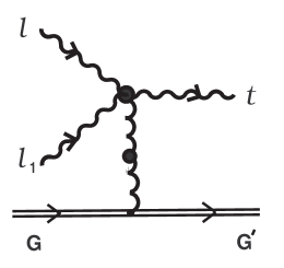
Figure 10: A scattering-fusion process of two soft-gluon longitudinal plasma excitations off energetic color particle with transition to one soft-gluon transverse plasma excitation.

These processes also need to be taken into account for total balance of energy losses. However, here, a new specific effect, namely for transverse mode is appeared. This is a possibility of large energy-momentum transfer from ultrarelativistic particle for scattering off plasmons with its conversion to transverse quantum of oscillations (see the last footnote). The energy of secondary quantum may be close to energy of initial hard particle. This is connected with that unlike longitudinal excitations, transverse ones have no restriction to maximum possible value of momentum of (8.12) type. However when energy of secondary quantum is close to energy of fast particle, then quantum effects become essential. Here, it is necessary to use quantum expressions for scattering processes on gluons of Compton’s type with change of incoming line of vacuum gluon by plasma gluon with longitudinal polarization, and a factor provides renormalization of a gluon wave function by thermal effects. The scattering on longitudinal gluons with conversion to hard transverse radiation produces additional mechanism imposed upon gluon bremsstrahlung. The processes of such a kind for usual (Abelian) plasma were first considered by Gailitis and Tsytovich in Ref. [54].

Finally, a last remark that should be mentioned, is concerned with energy loss of color dipole, next in order of complexity to color object after single color-charge particle. Classical color dipole can be considered as ‘toy’ model for heavy quarkonia ($c\bar{c}$ or $b\bar{b}$) propagating through QGP, and its energy loss may be relevant for the distortion of heavy-quarkonium production by plasma formation. Within linear response theory this problem was first considered by Koike and Matsui in Ref. [17]. However an attempt of direct extension of the result obtained by Koike and Matsui to the case of the scattering of color dipole off soft-gluon excitations of QGP encounter specific difficulties. In fact we can easily define expression for “starting” current generated by the color pairs. For a neutral pair, in the approximation ‘point’ dipole we have

$$\tilde{J}_{Q\bar{Q}}^{(0)a\mu}(p)=\frac{g}{(2\pi)^{3}}\,\tilde{v}^{\mu}\delta(\tilde{v}\cdot p)\,\frac{1}{2}\biggl{\{}\frac{\sqrt{1-{\tilde{\bf v}}^{2}}}{{\tilde{\bf v}}^{2}}\,({\bf p}\cdot\tilde{\bf v})({\bf d}^{a}\cdot\tilde{\bf v})+\frac{1}{{\tilde{\bf v}}^{2}}\,({\bf p}\times\tilde{\bf v})({\bf d}^{a}\times\tilde{\bf v})\biggr{\}},$$ (11.1)

where ${\bf d}^{a}=(Q^{a}_{10}-Q^{a}_{20}){\bf r}_{0}$ is the color dipole moment with fixed separation ${\bf r}_{0}$ of color charges in a intrinsic frame of reference, and $\tilde{\bf v}$ is a velocity of dipole. Substituting (11.1) into expression for energy loss (7.1), previously replacing

$$\int\!dQ\rightarrow\int\!dQ_{1}dQ_{2},\quad E_{Q}^{ai}(p)\rightarrow E_{Q\bar{Q}}^{ai}(p)=-i\omega\,^{\ast}{\cal D}^{i\nu}(p)\tilde{J}_{Q\bar{Q}\nu}^{\,a}[A^{(0)}](p),$$

we derive polarization energy loss for color dipole. To take into account scattering process for color dipole off soft plasma waves and energy loss associated with this process, we must calculate the next term in the expansion of effective color-dipole current $\tilde{J}_{Q\bar{Q}}^{\,a\mu}[A^{(0)}](p)$, linear over soft fluctuation field of system $A_{\mu}^{(0)a}$. The problem lies in the fact that not only a field of incident wave, but also field of second charge of pair are acted on each of color charge vectors of dipole. This circumstance very complicates and tangles the problem, compared to single color charge (see, e.g. work of Khriplovich [55] on construction of a field produced by two fixed Yang-Mills point charges), and therefore demands development of more refined method for calculating effective color-dipole current, that is out of the scope of the present study.

References

[1]
Yu.A. Markov and M.A. Markova, Ann. Phys. (N.Y.)302
(2002), 172.
[2]
E. Braaten and R.D. Pisarski, Nucl. Phys. B337 (1990), 569;
339 (1990), 310; J. Frenkel and J.C. Taylor, Nucl. Phys. B334 (1990), 199.
[3]
Yu.A. Markov and M.A. Markova, J. Phys. G26 (2000), 1581.
[4]
J.-P. Blaizot and E. Iancu, Nucl. Phys. B417 (1994), 608.
[5]
S.K. Wong, Nuovo Cimento A65 (1970), 689.
[6]
M. Gyulassy and M. Plümer, Phys. Lett. B243 (1990), 432;
Nucl. Phys. B346 (1990), 1; M. Gyulassy, M. Plümer, M. Thoma,
and X.-N. Wang, Nucl. Phys. A538 (1992), 37c.
[9]
R. Baier, Yu.L. Dokshitzer, A.H. Mueller, and D. Schiff, JHEP0109
(2001), 033.
[10]
X.-N. Wang, Phys. Rev. C63 (2001), 054902;
M. Gyulassy, I. Vitev, and X.-N. Wang, Phys. Rev. Lett.86 (2001),
2537; M. Gyulassy et al., Phys. Lett. B526 (2002), 301.
[11]
I.P. Lokhtin, A.M. Snigirev, and I. Vitev, CERN Yellow Report (2002),
hep-ph/0212061.
[12]
P. Levai et al., Nucl. Phys. A698 (2002), 631;
X.-N. Wang, Nucl. Phys. A702 (2002), 238;
E. Wang and X.-N. Wang, Phys. Rev. Lett.89 (2002), 162301.
[13]
T. Hirano and Y. Nara, Phys. Rev. C66 (2002), 041901;
S. Jeon, J. Jalilian-Marian, and I. Sarcevic, Phys. Lett.562
(2003), 45; Nucl. Phys. A723 (2003), 467.
[14]
M. Gyulassy, I. Vitev, X.-N. Wang, and B.-W. Zhang,
Review for Quark-Gluon Plasma 3, Editors: R.C. Hwa and X.-N. Wang,
Word Scientific, Singapore, 69p., nucl-th/0302077.
[16]
E. Braaten and M.H. Thoma, Phys. Rev. D44 (1991), 1298;
44 (1991), R2625.
[17]
M.H. Thoma and M. Gyulassy, Nucl. Phys. B351 (1991), 491;
St. Mrówczyński, Phys. Lett. B269 (1991), 383;
Y. Koike and T. Matsui, Phys. Rev. D45 (1992), 3237.
[19]
M. Gyulassy and X.-N. Wang, Nucl. Phys. B420 (1994), 583;
X.-N. Wang, M. Gyulassy, and M. Plümer, Phys. Rev. D51 (1995),
3436.
[20]
R. Baier, Yu.L. Dokshitzer, S. Peigné, and D. Schiff, Phys. Lett B
(1995), 277;
R. Baier, Yu.L. Dokshitzer, A.H. Mueller, S. Peigné and D. Schiff,
Nucl. Phys. B478 (1996), 577; 483 (1997), 291;
484 (1997), 265; 531 (1998), 403.
[21]
R. Baier, Yu.L. Dokshitzer, A.H. Mueller, and D. Schiff, Phys. Rev. C58 (1998), 1706; 60 (1999), 064902; 64 (2001), 057902.
[22]
R. Baier, D. Schiff, and B.G. Zakharov, Ann. Rev. Nucl. Part. Sci.50 (2000), 37.
[26]
A. Kovner and U.A. Wiedemann,
Review for Quark-Gluon Plasma 3, Editors: R.C. Hwa and X.-N. Wang,
Word Scientific, Singapore, 57p., hep-ph/0304151.
[27]
I.P. Lokhtin and A.M. Snigirev, Phys. Lett B440 (1998), 163;
Yad. Fiz.64 (2001), 1563;
Phys. Atom. Nucl.64 (2001), 1487.
[28]
M. Gyulassy, P. Lévai, and I. Vitev, Phys. Rev. Lett.85 (2000),
5535; Nucl. Phys. B571 (2000), 197; 594 (2001), 371;
Phys. Rev. D66 (2002), 014005.
[29]
X.F. Guo and X.-N. Wang, Phys. Rev. Lett.85 (2000), 3591;
Nucl. Phys. A696 (2001), 788; E. Wang and X.-N. Wang,
Phys. Rev. Lett.89 (2002), 162301;
B.-W. Zhang and X.-W. Wang, Nucl. Phys. A720 (2003), 429.
[30]
E.V. Shuryak and I. Zahed, Phys. Rev. D67 (2003), 054025;
E.V. Shuryak, hep-ph/0205031 (unpublished).
[31]
E. Wang and X.-N. Wang, Phys. Rev. Lett.87 (2001), 142301.
[33]
A.I. Akhiezer, I.A. Akhiezer, R.V. Polovin, A.G. Sitenko, and K.N. Stepanov,
“Plasma Electrodynamics”, Pergamon, New York, 1975.
[34]
A. Leonidov, Z. Phys. C66 (1995), 263.
[35]
P.A. Sturrock, Phys. Rev.141 (1966), 186.
[36]
A. Gailitis and V.N. Tsytovich, Zh. Eksp. Teor. Fiz.47 (1964),
1464; Sov. Phys.-JETP20 (1965), 987.
[37]
B. Svetitsky, Phys. Rev. D37 (1988), 2484.
[38]
M.G. Mustafa, D. Pal, D.K. Srivastava, Phys. Rev. C57
(1998), 889; D.B. Walton and J. Rafelski, Phys. Rev. Lett.84
(2000), 31.
[39]
M.G. Mustafa, D. Pal, D.K. Srivastava, and M. Thoma, Phys. Lett. B428 (1998), 234.
[40]
Yu. L. Dokshitzer and D.E. Kharzeev, Phys. Lett. B519 (2001),
199.
[41]
E. Shuryak, Phys. Rev. C55 (1997), 961;
Z. Lin, R. Vogt, and X.-N. Wang, Phys. Rev. C57 (1998), 899;
Z. Lin and R. Vogt, Nucl. Phys. B544 (1999), 339.
[42]
B. Kämpfer, O.P. Pavlenko, and K. Gallmeister, Phys. Lett. B419 (1998), 412; I.P. Lokhtin and A.M. Snigirev, Eur. Phys. J. C21 (2001), 155.
[43]
V.N. Tsytovich, “Non-linear Effects in Plasma,” Pergamon, Oxford, 1970;
V.N. Tsytovich, “Theory of a Turbulent Plasma,” Consultant Bureau, New York,
1977.
[44]
Yu.A. Markov, M.A. Markova, and A.N. Vall, Nonlinear dynamics of soft boson
excitations in hot QCD plasma III: Plasmon bremsstrahlung, in preparation.
[45]
J.-P. Blaizot and E. Iancu, Phys. Rep.359 (2002), 355;
B.J. Nauta and Ch.G. van Weert, ITFA-98-44, hep-ph/9901213 (unpublished).
[46]
H.A. Weldon, Phys. Rev. D28 (1983), 2007.
[47]
V.V. Lebedev and A.V. Smilga, Ann. Phys. (N.Y.)202 (1990), 229;
V.P. Silin and V.N. Ursov, Sov. Phys.-Lebedev Inst. Rep.5 (1988),
43.
[48]
F. Flechsig and A.K. Rebhan, Nucl. Phys. B464 (1996), 279.
[49]
U. Kraemmer, A.K. Rebhan, and H. Schulz, Ann. Phys. (N.Y.)238
(1995), 286.
[50]
V.V. Ochelkov, O.F. Prilutskij, I.L. Rozental, and V.V. Usov,
“Relativistic kinetics and hydrodynamics,” Atomizdat, Moscow, 1979.
[51]
E. Iancu, A. Leonidov, and L. McLerran, Nucl. Phys. A692
(2001), 583; E. Ferreiro, E. Iancu, A. Leonidov, and L. McLerran,
Nucl. Phys. A703 (2002), 489.
[52]
L. McLerran and R. Venugopalan, Phys. Rev. D49 (1994), 2233;
49 (1994), 3352; 50 (1994), 2225.
[53]
T. Altherr and D. Seibert, Phys. Lett. B333 (1994), 149;
T. Altherr, Phys. Lett. B341 (1995), 325;
P. Bedaque, Phys. Lett. B344 (1995), 23;
A. Niégawa, Phys. Lett. B416 (1998), 137;
I. Dadić, Phys. Rev. D59 (1999), 125012; 63 (2001),
25011; BI-TP 2000/14, IRB-TH-5/00, hep-ph/0103025;
F. Gelis, D. Schiff, and J. Serreau, Phys. Rev. D64 (2001),
056006.
[54]
A. Gailitis and V.N. Tsytovich, Zh. Eksp. Teor. Fiz.46 (1964),
1726; Sov. Phys.-JETP19
(1964), 1165.