Abstract

We study the decay of the neutral B meson to $K^{*}\gamma\gamma$ within the framework of the Standard Model, including long distance contributions.

—————————————————————————————————- We have corrected a sign error in the numerical program. The new estimates agree well with the ones given in a recent paper [15]
—————————————————————————————————

1 Introduction

Of late the rare decays of the B mesons have been recognized as important tools to study the basic structure and validity of the Standard Model (SM) and its extensions. In particular, the radiative decays, owing to their relative cleanliness as far as experimental signatures are concerned, have attracted a great deal of attention. For a general overview of the kind of issues considered relating to radiative decay modes, see [1, 2, 3] and references therein. The decays $B\to X_{s}\gamma$ and $B\to K^{*}\gamma$ have been observed [2] and both these are extensively used and relied upon for constrining the parameters of any new theory or extension of the SM [3]. The decay $B\to K^{*}\gamma\gamma$ is another potential testing ground for the effective quark level Hamiltonian $b\to s\gamma\gamma$ first studied by Lin, Liu and Yao [4] and pursued further in references [5],[6] and [7]. This amplitude has been the focus of considerable research recently, not only for the useful indications it will give to the underlying theories of flavour changing neutral currents, or the possible contributions from loops with supersymmetric partner particles, but for the impending experimental studies of the B-factories in the near future.

As has been previously noted, the $b\to s\gamma\gamma$ amplitude naturally splits into two categories: an irreducible contribution which is well known and usually estimated through basic triangle graphs, and a reducible one, where the second photon is attached to the external quark lines of the $b\to s\gamma$ amplitude. At the quark level the reducible contribution presents no real problems, however, when we consider an exclusive channel, such as $B\to M\gamma\gamma$ for a specific meson $M$, it becomes more appropriate to consider the second photon as arising from the external hadron legs of the amplitude $B\to M\gamma$. In contrast to the earlier cases of $B\to K(\pi)\gamma\gamma$ [7] where the amplitude for a single real photon vanishes identically, resulting in the irreducible diagram to be the sole contributor, the amplitude $B\to K^{*}\gamma$ is non vanishing. However for the neutral decay mode the second photon cannot arise from the resulting $K^{*}$, and thus in this case also, it is the irreducible amplitude that stands out, though for a completely different reason. Of course we must also consider the usual long distance contributions, such as the process $B\to K^{*}\eta_{c}$ followed by the decay $\eta_{c}\to\gamma\gamma$. Note that for completeness we will also include the $\eta$ contribution, even though the $\eta$ coupling to $\bar{c}c$ will be small. The rate for $B\to K\eta^{\prime}$ is anomalously high and many possible mechanisms have been proposed that aim at taking this anomalous production into account[8]. However, in the present case there is not enough data corresponding to the $B\to K^{*}\eta^{\prime}$ channel, and at present only an upper limit on this branching ratio is available. We therefore tend to remain conservative in the present study regarding this issue and assume that the $\eta^{\prime}$ contribution can be obtained similar to the $\eta_{c}$ contribution. The situation is expected to improve with the availability of more and precise data in this direction. We therefore include an $\eta^{\prime}$ contribution along the lines of the $\eta_{c}$ contribution.

In this paper we will estimate the branching ratio for the process $B^{0}\to K^{*0}\gamma\gamma$ by considering the effects of the irreducible triangle diagram contributions in the next section, followed by the resonance contributions in section 3. Note that in the case of $B\to K^{*}\gamma\gamma$ there will only be three sizeable resonance contributions; $\eta_{c}$, $\eta$ and $\eta^{\prime}$. Furthermore, each of these contributions will only contribute a narrow peak in the $\gamma\gamma$ invariant mass spectrum, which is easily separated experimentally. As such the interference terms for each of these pairs of terms will not be considered here. Finally in section 4 we will present our results and analysis.

2 The Irreducible Contributions

The irreducible triangle contributions to the process in which we are interested ($B\to K^{*}\gamma\gamma$) originate from the quark level process $b\to s\gamma\gamma$. The effective Hamiltonian for this process is [4]

$${\cal H}_{eff}=-\frac{G_{F}}{\sqrt{2}}V_{ts}^{*}V_{tb}\sum_{i}C_{i}(\mu)O_{i}(\mu),$$ (1)

with

$$O_{1} = (\bar{s}_{i}c_{j})_{V-A}(\bar{c}_{j}b_{i})_{V-A},$$

$$O_{2} = (\bar{s}_{i}c_{i})_{V-A}(\bar{c}_{j}b_{j})_{V-A},$$

$$O_{3} = (\bar{s}_{i}b_{i})_{V-A}\sum_{q}(\bar{q}_{j}q_{j})_{V-A},$$

$$O_{4} = (\bar{s}_{i}b_{j})_{V-A}\sum_{q}(\bar{q}_{j}q_{i})_{V-A},$$

$$O_{5} = (\bar{s}_{i}b_{i})_{V-A}\sum_{q}(\bar{q}_{j}q_{j})_{V+A},$$ (2)

$$O_{6} = (\bar{s}_{i}b_{j})_{V-A}\sum_{q}(\bar{q}_{j}q_{i})_{V+A},$$

$$O_{7} = \frac{e}{16\pi^{2}}\bar{s}_{i}\sigma^{\mu\nu}\left(m_{s}P_{L}+m_{b}P_{R}\right)b_{i}F_{\mu\nu},$$

$$\mathrm{and}\hskip 20.0ptO_{8} = \frac{g}{16\pi^{2}}\bar{s}_{i}\sigma^{\mu\nu}\left(m_{s}P_{L}+m_{b}P_{R}\right)T^{a}_{ij}b_{j}G^{a}_{\mu\nu}.$$

The invariant amplitude corresponding to this effective Hamiltonian is

$${\cal M}_{b\to s} = \left[\frac{16\sqrt{2}\alpha G_{F}}{9\pi}V_{ts}^{*}V_{tb}\right]\bar{u}(p_{s})\left\{\sum_{q}A_{q}J(m_{q}^{2})\gamma^{\rho}P_{L}R_{\mu\nu\rho}\right.$$

$$+iB\left(m_{s}K(m_{s}^{2})P_{L}+m_{b}K(m_{b}^{2})P_{R}\right)T_{\mu\nu}$$

$$\left.+C\left(-m_{s}L(m_{s}^{2})P_{L}+m_{b}L(m_{b}^{2})P_{R}\right)\epsilon_{\mu\nu\alpha\beta}k_{1}^{\alpha}k_{2}^{\beta}\right\}u(p_{b})\epsilon^{\mu}(k_{1})\epsilon^{\nu}(k_{2}),$$

where

$$R_{\mu\nu\rho}=k_{1\nu}\epsilon_{\mu\rho\sigma\lambda}k_{1}^{\sigma}k_{2}^{\lambda}-k_{2\mu}\epsilon_{\nu\rho\sigma\lambda}k_{1}^{\sigma}k_{2}^{\lambda}+(k_{1}.k_{2})\epsilon_{\mu\nu\rho\sigma}(k_{2}-k_{1})^{\sigma},$$

$$T_{\mu\nu}=k_{2\mu}k_{1\nu}-(k_{1}.k_{2})g_{\mu\nu},$$

$$A_{u}=3(C_{3}-C_{5})+(C_{4}-C_{6});\hskip 20.0ptA_{d}=\frac{1}{4}A_{u},$$ (4)

$$A_{c}=3(C_{1}+C_{3}-C_{5})+(C_{2}+C_{4}-C_{6}),$$ (5)

$$A_{s}=A_{b}=\frac{1}{4}[3(C_{3}+C_{4}-C_{5})+(C_{3}+C_{4}-C_{6})],$$

and

$$B=C=-\frac{1}{4}(3C_{6}+C_{5}).$$

In the above expressions we introduced the functions

$$J(m^{2})=I_{11}(m^{2}), K(m^{2})=4I_{11}(m^{2})-I_{00}(m^{2}), L(m^{2})=I_{00}(m^{2}),$$

where

$$I_{pq}(m^{2})=\int_{0}^{1}dx\int_{0}^{1-x}dy\frac{x^{p}y^{q}}{m^{2}-2(k_{1}.k_{2})xy-i\epsilon}.$$ (6)

Note that to get the ${\cal M}(B\to K^{*}\gamma\gamma)$ invariant amplitude from the quark level amplitude we replace the $\langle s|\Gamma|b\rangle$ by $\langle K^{*}|\Gamma|B\rangle$ for any Dirac bilinear $\Gamma$.

With $q=p_{B}-p_{K^{*}}=k_{1}+k_{2}$ and following Cheng et al. [9], we parameterize the hadronic matrix elements as

$$\langle K^{*}(p_{K^{*}})|\bar{s}\gamma_{\mu}b|B(p_{B})\rangle = \left(\frac{2V(q^{2})}{m_{B}+m_{K^{*}}}\right)\epsilon_{\mu\nu\alpha\beta}\epsilon^{*\nu}(p_{K^{*}})p_{B}^{\alpha}p_{K^{*}}^{\beta},$$ (7)

$$\langle K^{*}(p_{K^{*}})|\bar{s}\gamma_{\mu}\gamma_{5}b|B(p_{B})\rangle = i\left[(m_{B}+m_{K^{*}})\epsilon^{*\mu}(p_{K^{*}})A_{1}(q^{2})\right.$$

$$-\frac{\epsilon^{*}.p_{B}}{m_{B}+m_{K^{*}}}(p_{B}+p_{K^{*}})_{\mu}A_{2}(q^{2})$$

$$\left.-2\frac{m_{K^{*}}}{q^{2}}(\epsilon^{*}.p_{B})q_{\mu}\left\{A_{3}(q^{2})-A_{0}(q^{2})\right\}\right],$$

For the functional dependence of various form factors appearing above, we follow [10]. Using these definitions, we determine the irreducible matrix element for the process $B\to K^{*}\gamma\gamma$ as

$${\cal M}_{irr}=\left(\frac{16\sqrt{2}\alpha G_{F}}{9\pi}\right)\epsilon^{\mu}(k_{1})\epsilon^{\nu}(k_{2})\left[{\cal M}^{(1)}_{\mu\nu}+{\cal M}^{(2)}_{\mu\nu}+{\cal M}^{(3)}_{\mu\nu}\right]$$ (9)

where

$${\cal M}^{(1)}_{\mu\nu} = R_{\mu\nu\rho}\left.\Bigg{[}K_{A1}\epsilon^{\rho\alpha\beta\gamma}\epsilon^{*}_{K^{*}\alpha}p_{B\beta}p_{K^{*}\gamma}-K_{A2}\epsilon^{*\rho}_{K^{*}}\right.$$

$$\left.+K_{A3}(\epsilon^{*}_{K^{*}}.p_{B})(p_{B}+p_{K^{*}})^{\rho}+K_{A4}(\epsilon^{*}_{K^{*}}.p_{B})q^{\rho}\Bigg{]}\right.$$

$${\cal M}^{(2)}_{\mu\nu} = K_{B}\left(k_{1\mu}k_{2\nu}-(k_{1}.k_{2})g_{\mu\nu}\right)(\epsilon^{*}_{K^{*}}.p_{B})$$ (10)

$${\cal M}^{(3)}_{\mu\nu} = K_{C}\epsilon_{\mu\nu\alpha\beta}k_{1}^{\alpha}k_{2}^{\beta}(\epsilon^{*}_{K^{*}}.p_{B})$$

The functions $K_{i}$ above are defined as

$$K_{A1}=\left[\sum_{q}A_{q}J(m_{q}^{2})\right]\frac{V(q^{2})}{m_{B}+m_{K^{*}}} K_{A2}=\left[\sum_{q}A_{q}J(m_{q}^{2})\right]\frac{i}{2}(m_{B}+m_{K^{*}})A_{1}(q^{2})$$ ;

$$K_{A3}=\left[\sum_{q}A_{q}J(m_{q}^{2})\right]\frac{i}{2}\frac{A_{1}(q^{2})}{m_{B}+m_{K^{*}}} K_{A4}=\left[\sum_{q}A_{q}J(m_{q}^{2})\right]\frac{im_{K^{*}}^{2}}{q^{2}}\left(A_{3}(q^{2})-A_{0}(q^{2})\right)$$ ;

and

$$K_{B} = -\frac{Bm_{K^{*}}}{m_{B}+m_{K^{*}}}A_{0}(q^{2})\left[m_{s}K(m_{s}^{2})-m_{b}K(m_{b}^{2})\right]$$

$$K_{C} = -\frac{iCm_{K^{*}}}{m_{B}+m_{K^{*}}}A_{0}(q^{2})\left[m_{s}L(m_{s}^{2})+m_{b}L(m_{b}^{2})\right].$$

3 Resonance contributions

For this process there will be three significant resonance contributions, that from the $\eta_{c}$-, $\eta$- and $\eta^{\prime}$-resonances. The $\eta_{c}$ contribution to the decay process comes via the $t$-channel decay $B\to K^{*}\eta_{c}$, with the $\eta_{c}$ then decaying into two photons.

The T-matrix element for this process can be written as

$$\langle K^{*}\gamma\gamma|T|B\rangle=-\frac{\langle K^{*}\eta_{c}|T|B\rangle\langle\gamma\gamma|T|\eta_{c}\rangle}{q^{2}-m_{\eta_{c}}^{2}+im_{\eta_{c}}\Gamma_{total}^{\eta_{c}}}.$$ (11)

The amplitude $\langle\gamma\gamma|T|\eta_{c}\rangle$ is parameterized as [6]

$$\langle\gamma\gamma|T|\eta_{c}\rangle=2iB_{\eta_{c}}\epsilon^{\mu\nu\alpha\beta}\epsilon_{\mu}^{*}(k_{1})\epsilon_{\nu}^{*}(k_{2})k_{1\alpha}k_{2\beta}.$$ (12)

Note that we can determine $B_{\eta_{c}}$ from the known decay rate:

$$\Gamma(\eta_{c}\to\gamma\gamma)=\left(\frac{1}{2}\right)\frac{1}{2m_{\eta_{c}}}\int\frac{d^{3}k_{1}}{(2\pi)^{3}2k_{1}^{0}}\frac{d^{3}k_{2}}{(2\pi)^{3}2k_{2}^{0}}(2\pi)^{2}\delta^{(4)}(k_{\eta_{c}}-k_{1}-k_{2})\left|\langle\gamma\gamma|T|\eta_{c}\rangle\right|^{2},$$ (13)

where we have

$$\sum_{spins}\left|\langle\gamma\gamma|T|\eta_{c}\rangle\right|^{2}=2|B_{\eta_{c}}|^{2}q^{4},$$ (14)

and so

$$\Gamma(\eta_{c}\to\gamma\gamma)=\frac{|B_{\eta_{c}}|^{2}m_{\eta_{c}}^{3}}{16\pi}.$$ (15)

The $B\to K^{*}\eta_{c}$ amplitude has been determined in Cheng et al. [9] as

$${\cal M}(B\to K^{*}\eta_{c})=\frac{G_{F}}{\sqrt{2}}V_{cb}V_{cs}^{*}\left(C_{1}+\frac{1}{3}C_{2}\right)X_{C}^{(B_{0}K^{*0},\eta_{c})}$$ (16)

where

$$X_{C}^{(B_{0}K^{*0},\eta_{c})}=2f_{\eta_{c}}m_{K^{*}}A_{0}^{BK^{*}}(m_{\eta_{c}}^{2})(\epsilon^{*}_{K^{*}}.p_{B}).$$ (17)

Note that $f_{\eta_{c}}$ is defined as $\langle 0|\bar{c}\gamma_{\mu}c|\eta_{c}\rangle=if_{\eta_{c}}p_{\mu}(\eta_{c})$.

In the above way of parametrizing the $B\to K^{*}\eta_{c}$, there is a lot of model dependence that goe in. Since, the branching fractions for this sub-process is known, we can in principle avoid such a model dependnce by writing the amplitude as

$${\cal M}(B\to K^{*}\eta_{c})=a^{\eta_{c}}_{eff}(\epsilon^{*}_{K^{*}}.p_{B})$$ (18)

and determine the effective constant from the corresponding decay rate. We folow this procedure and therefore try to avoid any model dependence as far as possible.

Therefore the total contribution due to the $\eta_{c}$ resonances is thus,

$${\cal M}_{\eta_{c}}=2B_{\eta_{c}}a^{\eta_{c}}_{eff}\frac{(\epsilon_{K^{*}}.p_{B})}{q^{2}-m_{\eta_{c}}^{2}+im_{\eta_{c}}\Gamma_{total}^{\eta_{c}}}\epsilon^{\mu\nu\alpha\beta}\epsilon^{*}_{1\mu}\epsilon^{*}_{2\nu}k_{1\alpha}k_{2\beta}.$$ (19)

Analogous to the $\eta_{c}$ resonance, the $\eta$- and $\eta^{\prime}$-resonance contributions, ${\cal M}_{\eta}$ and ${\cal M}_{\eta^{\prime}}$, have exactly the same form as equation (19) with the parameters $B_{\eta_{c}}$, $m_{\eta_{c}}$ and $\Gamma_{total}^{\eta_{c}}$ being replaced by their $\eta$- and $\eta^{\prime}$-counterparts respectively. However in this case we cannot define the relative sign of the amplitudes and any of the other components of the amplitude.

The process can also receive additional contribution from the $B^{*}$ and $K_{2}^{*}$ channels where the B meson decays into a photon and an on-shell $K_{2}^{*}$ or slightly off-shell $B^{*}$ and then these giving rise to $K^{*}$ and the second photon. However, there is no data available at present for either of these and if the widths for the individual channels contributing to the process are significant, the contribution can be sizeable. However, we expect that these contributions can be eliminated by suitable cuts in the $B^{*}$- (or $K_{2}^{*}$-) photon plane and thus we do not consider them here at all.

4 Results

The squared amplitude for the process $B\to K^{*}\gamma\gamma$ is then;

$$\left|M_{tot}\right|^{2}=\left|M_{irr}\right|^{2}+\left|M_{\eta_{c}}\right|^{2}+\left|M_{\eta}\right|^{2}+\left|M_{\eta^{\prime}}\right|^{2}$$ (20)

where the interference terms have not been included here. The components to the squared amplitude were calculated to be;

$$\sum_{spins}\left|M_{\eta_{c}}\right|^{2}=\left|R\right|^{2}\lambda(s_{\gamma\gamma},m_{B}^{2},m_{K^{*}}^{2})\frac{q^{4}}{8m_{K^{*}}^{2}},$$ (21)

where

$$R = 2B_{\eta_{c}}a^{\eta_{c}}_{eff}\left[\frac{1}{q^{2}-m_{\eta_{c}}^{2}+im_{\eta_{c}}\Gamma_{tot}^{\eta_{c}}}\right],$$

$$\mathrm{and}\hskip 10.0pt\lambda(s_{\gamma\gamma},m_{B}^{2},m_{K^{*}}^{2}) = 4\left((p_{B}.p_{K^{*}})^{2}-m_{K^{*}}^{2}m_{B}^{2}\right).$$ (22)

We have similar expressions for the $\eta$ and $\eta^{\prime}$ terms, replacing the parameters $B_{\eta_{c}}$, $m_{\eta_{c}}$ and $\Gamma_{total}^{\eta_{c}}$ by their $\eta$ and $\eta^{\prime}$ counterparts.

The irreducible squared matrix element is then;

$$\sum_{spins}\left|M_{irr}\right|^{2} = \left[\frac{16\sqrt{2}\alpha G_{F}}{9\pi}V_{tb}V^{*}_{ts}\right]^{2}\frac{q^{4}}{2m_{K^{*}}^{2}}\left((p_{B}.p_{K^{*}})^{2}-m_{K^{*}}^{2}m_{B}^{2}\right)$$ (27)

$$\hskip 20.0pt\times\left[\begin{array}[]{c}\left|K_{A2}\right|^{2}+\left|K^{\prime}_{A3}\right|^{2}+\left|K^{\prime}_{A4}\right|^{2}+\left|K_{B}\right|^{2}+\left|K_{C}\right|^{2}\\ +2\mathrm{Re}(K_{A5})+2\mathrm{Re}(K^{\prime}_{A3}K^{*\prime}_{A4})\\ -2\mathrm{Re}(K_{A2}K^{*\prime}_{A3})-2\mathrm{Re}(K_{A2}K^{*\prime}_{A4})\end{array}\right]$$

where

$$K^{\prime}_{A3}=K_{A3}(m_{B}^{2}-m_{K^{*}}^{2}) K^{\prime}_{A4}=K_{A4}q^{2}$$ ;

$$K_{A5}^{*} = K^{*}_{C}\left[\sum_{q}A_{q}J(m_{q}^{2})\right]im_{K^{*}}A_{0}(q^{2})$$ (28)

The total decay rate is then given by

$$\frac{d\Gamma}{d(\cos\theta)d\sqrt{s_{\gamma\gamma}}}=\sqrt{s_{\gamma\gamma}}\left(\frac{1}{512m_{B}\pi^{3}}\right)\left[\left(1-\frac{s_{\gamma\gamma}}{m_{B}^{2}}+\frac{m_{K^{*}}^{2}}{m_{B}^{2}}\right)^{2}-\frac{4m_{K^{*}}^{2}}{m_{B}^{2}}\right]^{1/2}\sum_{spins}\left|{\cal M}\right|^{2},$$ (29)

where $\sqrt{s_{\gamma\gamma}}$ is the C.M. energy of the two photons while $\theta$ is the angle which the decaying B-meson makes with the two photons in the $\gamma\gamma$ C.M. frame.

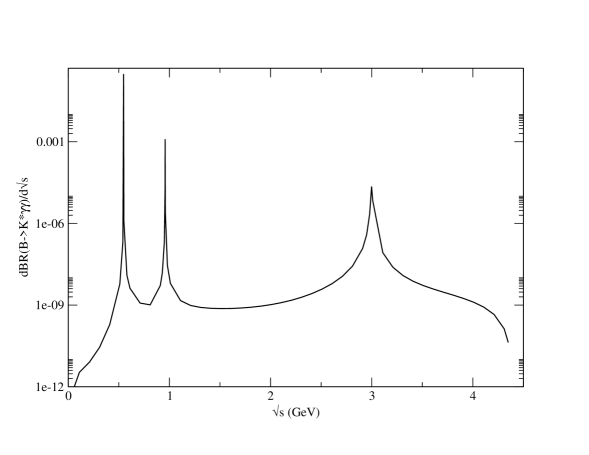
Figure 1: The differential branching ratio of $B\to K^{*}\gamma\gamma$ plotted as a function of the CM energy of the diphoton rest frame without interference terms taken into consideration. Here we have plotted with a log scale on the y-axis.

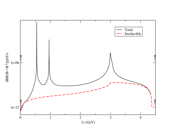
Figure 2: The irreducible and the total contribution to the differential branching ratio of $B\to K^{*}\gamma\gamma$ plotted as a function of the CM energy of the diphoton rest frame.

Our results are presented in figures 1 and 2 (both plotted with a logarithmic scale on the y-axis), where figure 1 shows the differential branching ratio given as a function of the invariant mass of the two photons, for the case of the neutral B meson decay without the interference terms between the resonances and the irreducible background included. The inclusion of the interference terms will in principle give rise to an interference pattern near the base of the resonance peaks. Since the peaks are narrow and moreover the interference contributions being small (except the $\eta_{c}$-Irreducible term), we do not include them in the plots. It is worth mentioning that imposition of suitable cuts in the spectrum to eliminate the resonance contributions will eliminate any such interference patterns also. The numerical estimate for the branching ratio arising due to all possible contributions is summarized in Table 1. Quite evidently, the largest contribution comes from the $\eta$ resonance mode. It should be stressed again that using appropriate cuts in the spectrum, the resonances can be completely eliminated and what is left is the background irreducible contribution. In estimating the numerical values for the interference terms, we have assumed that the relative signs between the terms are such that the $\eta$-Irreducible and $\eta^{\prime}$-Irreducible interfering contributions add on to the other pieces. However, because of the smallness of these values, it really makes no significant difference.

Contribution	Branching ratio $\times 10^{-7}$
Resonance
$\eta_{c}$	4.7
$\eta$	56.9
$\eta^{\prime}$	3.7
Irreducible	$2.3\times 10^{-2}$
Interference
$\eta_{c}$-Irreducible	2.6
$\eta$-Irreducible	$3\times 10^{-3}$
$\eta^{\prime}$-Irreducible	$4.5\times 10^{-3}$
BR	57.5

Table 1: Contribution to the $B^{0}\to K^{*0}\gamma\gamma$ branching ratio. For the interference terms we quote the absolute values.

In figure 2, we compare the irreducible contribution with the total contribution to the branching fraction. Clearly, the resonances dominate the results. At this point, it may be worth mentioning that a quick look at the individual values tabulated in Table1 reveal the following. Since the resonances are narrow, one may try to estimate the contributions directly by multiplying the individual branching ratios ie we expect in the narrow width approximation that $BR(B-->K^{*}\gamma\gamma)\sim BR(B-->K^{*}X)BR(X-->\gamma\gamma)$ where $X$ denotes any of the resonances. The numbers quoted clearly show that they are in accord with the expectations. However, if we had used the form as in Eq(17), we might have over- or under-estimated the resonance contributions (except probably for the $\eta$ mode) because it is not very clear if such a simple parametrization is the correct one. We however avoid any such possible conflict by drawing heavily on the experimental values (upper limit for $\eta^{\prime}$) of the various sub-process branching fractions.

The central values of the parameters used in our calculation are shown in the Appendix. We make an attempt to estimate the errors creeping into the numerical calculations due to errors in various input parameters. The theoretical uncertainties arising out of uncertainties in the parameters are overwhelmingly in the input values of the form factors and the meson decay constants . The Wilson coefficients have been taken to be their NNL values and there are no significant theoretical uncertainties in them. In evaluating the uncertainties of our results, it is appropriate to evaluate them separately for the background irreducible contribution and the resonance contributions, since the latter can easily be experimentally separated from the former by suitable cuts in the spectrum. For the model dependent parametrization of Eq(17), the theoretical uncertainty in the resonance contribution due to $\eta_{c}$ arises mostly because of uncertainties in the CKM parameters, $f_{\eta_{c}}$, $B_{\eta_{c}}$ and $F_{0}(m_{\eta_{c}^{2}})$; the Wilson coefficients values used are the NNL level values and no comparable uncertainties exist therein. The CKM parameters relevant to us have an uncertainty of about 10$\%$ [11]. The form factors used are the same as in [9] where the actual dependence of the form factors as a function of momentum transfer squared are given and hence no errors arise due to parametrization of form factors as a function of $q^{2}$. Although this reference does not quote any estimate of the uncertainties in the numbers, a typical uncertainty in this type of calculation based on quark model is given in [12] and is typically of the order of 15$\%$ ,arising to a great extent due to uncertainty in the strange quark mass. The rate of the $\eta_{c}$ decay into two photons is uncertain by about 40$\%$ [11]. A typical estimate of the uncertainty in the value of $f_{\eta_{c}}$( arising mostly again out of uncertainty in the current mass of the s-quark ) has been estimated at about 15$\%$ in [13]. Combining all this , we would expect that an estimate of the contribution of the $\eta_{c}$ resonance based on such a parametrization to be uncertain by about 50$\%$. A similar estimate for the other two resonaces give a somewhat lower value mostly because their decay rates into two photons is better known, to an accuracy of about 10 $\%$ for $\eta^{\prime}$ and about 5 $\%$ for the $\eta$. The uncertainties in the decay constansts of the $eta^{\prime}$ and the $\eta$ have been estimated to be about 10$\%$ [14] and we estimate the overall uncertainty in our calculation for the $\eta^{\prime}$ and $\eta$ to be about 40$\%$ and 30$\%$ respectively. However, since we have relied on experimental values of rates and branching fractions, the above mentioned uncertainties are significantly reduced and the only source of uncertainty in our estimation is the uncertainty present in sub-process rates.

Turning to the irreducible contribution, the uncertainty arises mostly because of the CKM factors and the form factors. These combine to give an overall uncertainty of about 20$\%$ for the irreducible part of the amplitude. As stressed before, once the suitable cuts are imposed in the two photon spectrum, it is possible to extract the irreducible contribution and here the errors are relatively smaller and are expected to even go down further with more accurate determination of the CKM parameters and the form factors.

At the levels reached by the current B-factories, the branching ratios obtained are too low to be observed. One certainly hopes that in the near future experiments, with better luminosities possible, the numbers obtained will be very useful for confronting theoretical models with experimental data. As discussed in the text, this decay with two photons depends on the parts of the effective Hamiltonian, which the decays with a single photon are not sensitive to and thus provides a more complete test of the underlying theory.

Acknowledgements   SRC would like to acknowledge the Department of Science and Technology, Government of India for a research grant.
We would like to thank Prof. G.Hiller for a communication pointing out the discrepancies between their results and our earlier estimates for the irreducible contribution.

5 Appendix

We list the central values of the various parameters entering our numerical estimates:

$$G_{F}=1.16x10^{-5}Gev^{-2}\hskip 28.45274pt\alpha(m_{B})=1/130\hskip 28.45274ptm_{b}=4.8Gev$$

$$m_{t}=175Gev\hskip 28.45274ptm_{c}=1.5Gev\hskip 28.45274ptm_{u}=0=m_{d}$$

$$m_{K^{*+}}=0.89Gev\hskip 28.45274ptm_{K^{*0}}=0.896Gev$$

$$F_{0}^{BK^{*}}=0.3\hskip 28.45274ptM_{pole}=6.65Gev$$

$$\Gamma_{tot}(\eta_{c})=1.3\times 10^{-2}\hskip 28.45274ptm_{\eta_{c}}=3.0Gev$$

$$B_{\eta_{c}}=2.74\times 10^{-3}Gev^{-1}\hskip 28.45274ptf_{\eta_{c}}=0.35Gev$$

$$\Gamma_{tot}(\eta^{\prime})=0.203\times 10^{-3}Gev\hskip 28.45274ptm_{\eta^{\prime}}=0.96Gev$$

$$B_{\eta^{\prime}}=14.0\times 10^{-3}Gev^{-1}\hskip 28.45274ptf_{\eta^{\prime}}=-6.3Mev$$

$$B(\eta^{\prime}\rightarrow 2\gamma)=2.11\%\hskip 28.45274ptB(\eta_{c}\rightarrow 2\gamma)=3\times 10^{-4}$$

References

• [1] B. Grinstein, R. Springer and M. Wise, Nucl. Phys. B339, 269 (1990); M. Misiak, Nucl. Phys. B393, 23 (1993); M. Ciuchini, E. Franco, G. Martinelli, L. Reina and L. Silvestrini, Nucl. Phys. B421, 41 (1994); K. Adel and Y. P. Yao, Phys. Rev. D49, 4945 (1994); C. Greub and T. Hurth, Phys. Rev. D56, 2934 (1997); A. Ali and C. Greub, Phys. Lett. B259, 182 (1991); K. G. Chetyrkin, M. Misiak and M. Munz, Phys. Lett. B400, 206 (1997); A. J. Buras, M. Misiak, M. Munz and S. Pokorski, Nucl. Phys. B424, 374 (1994); A. F. Falk, M. Luke and M. J. Savage, Phys. Rev. D49, 3367 (1994); A. Khodjamirian, R. Ruckl, G. Stoll and D. Wyler, Phys. Lett. B402, 167 (1997).
• [2] CLEO Collaboration, M. S. Alam et al, Phys. Rev. Lett. 74, 2885 (1995); CLEO Collaboration, R. Ammar et al, ibid 71, 674 (1993).
• [3] D. Pirjol, hep-ph/0207095; E. O. Iltan, New. J. Phys. 4, 54 (2002); K. Agashe, N. G. Deshpande and G. H. Wu, Phys. Lett. B514, 309 (2001); M. Carena, D. Garcia, U. Nierste and C. E. M. Wagner, Phys. Lett. B499, 141 (2001); D. Chakraverty and D. Choudhury, Phys. Rev. D63, 075009 (2001); R. Barbieri and G. F. Giudice, Phys. Lett. B309, 86 (1993); J. L. Lopez, D. V. Nanopoulos, X. Wang and A. Zichichi, Phys. Rev. D51, 147 (1995).
• [4] G.L.Lin, J.Liu and Y.P.Yao, Phys.Rev.Lett. 64, 1498 (1990); G.L.Lin, J.Liu and Y.P.Yao, Phys.Rev. D42, 2314 (1990).
• [5] C.V.Chang, G.Lin and Y.P.Yao, Phys.Lett. B415, 395 (1997).
• [6] L.Reina, G.Riccardi and A.Soni, Phys.Lett. B396, 231 (1997); Phys.Rev. D56, 5805 (1997).
• [7] S.R.Choudhury, G.C.Joshi, N.Mahajan and B.H.J.McKellar, Phys. Rev. D67, 074016 (2003); S.R.Choudhury, G.C.Joshi, N.Mahajan and B.H.J.McKellar, hep-ph/0306293.
• [8] M. R. Ahmady, E. Kou and A. Sugamoto, Phys. Rev. D57, 1997 (1998); D. Atwood and A. Soni, Phys. Lett. B405, 150 (1997); I. Halprin and A. Zhitnisky, Phys. Rev. Lett. 80, 438 (1998); I. Halprin and A. Zhitnisky, Phys. Rev. D56, 7247 (1997); F. Yuan and K. T. Chao, Phys. Rev. D56, 2495 (1997); W. -S. Hou and B. Tseng, Phys. Rev. Lett. 80, 434 (1998).
• [9] H.Y.Cheng, C.Y.Cheung and C.W.Hwang, Phys.Rev. D55, 1559 (1997).
• [10] A. Ali, P. Ball, L. T. Handoko and G. Hiller, Phys. Rev. D61, 074024 (2000).
• [11] K. Hagiwara etal., Particle Data Group, Phys. Rev. D66, 010001 (2002).
• [12] M. Beneke and M. Neubert, hep-ph/0308039.
• [13] N. G. Deshpande and J. Trampetic, Phys. Lett. B339, 270 (1994).
• [14] Y-H. Chen, H-Y. Cheng, B. Tsing and K-C. Yang, Phys. Rev. D60, 094014 (1999).
• [15] G. Hiller and A. Safir, hep-ph/0411344.
Refer to caption