Evaluation of two-loop self-energy basis integrals using differential equations

Abstract

I study the Feynman integrals needed to compute two-loop self-energy functions for general masses and external momenta. A convenient basis for these functions consists of the four integrals obtained at the end of Tarasov’s recurrence relation algorithm. The basis functions are modified here to include one-loop and two-loop counterterms to render them finite; this simplifies the presentation of results in practical applications. I find the derivatives of these basis functions with respect to all squared-mass arguments, the renormalization scale, and the external momentum invariant, and express the results algebraically in terms of the basis. This allows all necessary two-loop self-energy integrals to be efficiently computed numerically using the differential equation in the external momentum invariant. I also use the differential equations method to derive analytic forms for various special cases, including a four-propagator integral with three distinct non-zero masses.

I Introduction

The comparison of data with the predictions of the Standard Model, and candidate extensions of it, requires the kind of accuracy obtained from two-loop and even higher-order calculations. As a forward-looking example, if supersymmetry proves to be correct then the Large Hadron Collider will be able to measure the mass of the lightest neutral Higgs scalar boson to an accuracy of order 100 MeV, and a future linear collider will certainly do better Higgsexp . In contrast, even assuming perfect knowledge of all input parameters, the present theoretical uncertainty is probably at least 10 times larger Higgstheory .

The motivation for the present paper is to facilitate routine calculations of self-energies, and thus pole masses, for particles in any field theory. A key step in this process is the evaluation of the necessary two-loop integrals. It has become clear that analytical methods will only work in special cases, so practical numerical methods are needed. In this paper, I will build on the many important advances that have been made in this area Tarasov:1997kx -Mertig:1998vk , with the goal of streamlining both computations and presentations of results for self-energies.

Tarasov Tarasov:1997kx has provided a solution to the problem of reducing two-loop self-energy integrals to a minimal basis, such that any scalar integral can be represented as a linear combination of integrals of just four types, plus terms quadratic in one-loop integrals. (Other useful reduction algorithms are presented in Weiglein:hd and Ghinculov:1997pd .) Tarasov’s algorithm relies on the integration by parts technique Tkachov:wb and repeated use of recurrence relations involving integrals in different numbers of dimensions Tarasov:1996br . The two-loop scalar basis integrals remaining after applying this algorithm have the topologies shown in Figure 1.

Figure 1: Feynman diagrams for the two-loop basis integrals.

They are the three-propagator “sunrise” diagram $S$, a diagram $T$ which is obtained from the sunrise diagram by differentiating with respect to one of the squared masses, a four-propagator diagram $U$, and the five-propagator “master” Broadhurst:1987ei diagram $M$.

Consider a generic two-loop integral $F_{i}(s;x,y,\ldots)$, which depends on the external momentum invariant

$$s=-p^{2},$$ (1.1)

[using either a Euclidean or a signature ($-$$+$$+$$+$) metric] and propagator squared masses $x,y,\ldots$. For special values of the arguments, it may be possible to compute $F_{i}$ analytically in terms of polylogarithmsLewin or Nielsen’s generalized polylogarithmsKolbig . This requires Scharfthesis that there is no three-particle cut of the diagram for which the three cut masses $m_{1},m_{2},m_{3}$, the invariant $\hat{s}$ for the total momentum flowing across the cut, and the four quantities

$$\hat{s}-(m_{1}\pm m_{2}\pm m_{3})^{2}$$ (1.2)

are all non-zero. Many analytical results for various such special cases have been worked out Rosner -Martin:2001vx . There are also expansions Smirnov:rz -Berends:1994sa in large and small values of the external momentum invariant, and near the thresholds and pseudo-thresholds Berends:1996gs -Groote:2000kz . Integral representations Kreimer:1991jv -Passarino:2001wv allow for systematic numerical evaluations.

In this paper I rely instead on the differential equation method Kotikov:1990kg -Caffo:2002wm for evaluating the basis integrals. The idea is to take advantage of the fact that the basis integrals $F_{i}$ satisfy a set of coupled first-order linear ordinary differential equations in $s$, of the form

$$s\frac{d}{ds}F_{i} = \sum_{j}C_{ij}F_{j}+C_{i}.$$ (1.3)

Here $C_{ij}$ and $C_{i}$ are ratios of polynomials in $s$ and the squared masses. (If we include only genuine two-loop functions in the set $F_{i}$, then $C_{i}$ will also include terms linear and quadratic in the one-loop functions, which are known analytically and present no problems.) The values of the functions $F_{i}$ are known analytically at $s=0$. So one can integrate the differential equations from the initial conditions at $s=0$ to the desired value of $s$ using well-known numerical techniques such as Runge-Kutta. For the integrals of the type $S,T,U$, this has already been done and explained in detail in Caffo:1998du -Caffo:2002wm . Here, I will extend these results to include the master integral $M$, and present results for $S,T,U$ integrals in a different basis which may be more convenient for some purposes.

In order to find the differential equations in $s$ that the basis integrals satisfy, I proceed by first calculating the derivatives of the basis integrals with respect to their propagator squared-mass arguments. Using Tarasov’s recurrence relations, these derivatives are expressed algebraically in terms of the basis functions, in the linear form:

$$\frac{\partial}{\partial x}F_{i} = \sum_{j}K_{xij}F_{j}+K_{xi}.$$ (1.4)

The equations (1.3) in $s$ will then follow by elementary dimensional analysis, using the known dependence of the basis functions on the renormalization scale. The derivatives of the basis functions with respect to the squared masses are also useful in their own right, since each derivative adds an extra power of the corresponding propagator in the denominator. This provides a simplified algebraic algorithm for computing integrals with arbitrary powers of the propagators present in the master integral topology.

The rest of this paper is organized as follows. Section II defines the basis integrals, and gives conventions and notations. Section III presents the derivatives of the basis integrals with respect to their squared-mass arguments. In section IV, I give the differential equations in $s$ satisfied by the basis functions. The numerical integration of the differential equations near $s=0$ relies on expansions for small $s$, which are provided in section V. Section VI presents some analytic expressions for the basis functions in special cases that are useful both for comparison with the literature and for practical purposes. Section VII describes the numerical computation of the basis integrals, and gives two examples.

II Conventions and Setup

The loop functions in this papers are defined by scalar Euclidean momentum integrals regularized by dimensional reduction to $d=4-2\epsilon$ dimensions. Let us define a loop factor

$$C=(16\pi^{2})\frac{\mu^{2\epsilon}}{(2\pi)^{d}}=(2\pi\mu)^{2\epsilon}/\pi^{2}.$$ (2.1)

The regularization scale $\mu$ is related to the renormalization scale $Q$ (in the $\overline{\rm MS}$ scheme msbar , or the $\overline{\rm DR}$ scheme drbar for supersymmetric theories, or in the $\overline{\rm DR}^{\prime}$ scheme drbarprime for softly broken supersymmetric theories) by

$$Q^{2} = 4\pi e^{-\gamma}\mu^{2}.$$ (2.2)

Logarithms of dimensionful quantities are always given in terms of

$${\overline{\rm ln}}X \equiv {\rm ln}(X/Q^{2}).$$ (2.3)

The loop integrals are functions of a common external momentum invariant $s$ as explained in the Introduction. (Note that the sign convention is such that for a stable physical particle with mass $m$, there is a pole at $s=m^{2}$.) Throughout this paper, $s$ should be taken to have an infinitesimal positive imaginary part. Since all functions in any given equation have the same $s$, it will not be included explicitly in the list of arguments.

The one-loop self-energy integrals Passarino:1978jh are defined as:

$${\bf A}(x) = C\int d^{d}k\frac{1}{[k^{2}+x]},$$ (2.4)

$${\bf B}(x,y) = C\int d^{d}k\frac{1}{[k^{2}+x][(k-p)^{2}+y]}.$$ (2.5)

The two-loop integrals are defined as:

$${\bf S}(x,y,z) = C^{2}\int d^{d}k\int d^{d}q\frac{1}{[k^{2}+x][q^{2}+y][(k+q-p)^{2}+z]},$$ (2.6)

$${\bf T}(x,y,z) = -\frac{\partial}{\partial x}{\bf S}(x,y,z),$$ (2.7)

$${\bf U}(x,y,z,u) = C^{2}\int d^{d}k\int d^{d}q\frac{1}{[k^{2}+x][(k-p)^{2}+y][q^{2}+z][(q+k-p)^{2}+u]},$$ (2.8)

$${\bf M}(x,y,z,u,v) = C^{2}\int d^{d}k\int d^{d}q\frac{1}{[k^{2}+x][q^{2}+y][(k-p)^{2}+z][(q-p)^{2}+u][(k-q)^{2}+v]}.$$ (2.9)

I find it convenient to introduce modified integrals in which appropriate divergent parts have been subtracted. At one-loop order, define the finite and $\epsilon$-independent integrals:

$$A(x) = \lim_{\epsilon\rightarrow 0}\left[{\bf A}(x)+x/\epsilon\right]=x(\overline{\rm ln}x-1),$$ (2.10)

$$B(x,y) = \lim_{\epsilon\rightarrow 0}\left[{\bf B}(x,y)-1/\epsilon\right]=-\int_{0}^{1}dt\>{\overline{\rm ln}}[tx+(1-t)y-t(1-t)s].$$ (2.11)

At two loops, let

$$S(x,y,z) = \lim_{\epsilon\rightarrow 0}\left[{\bf S}(x,y,z)-S^{(1)}_{\rm div}(x,y,z)-S^{(2)}_{\rm div}(x,y,z)\right],$$ (2.12)

where

$$S^{(1)}_{\rm div}(x,y,z) = \left({\bf A}(x)+{\bf A}(y)+{\bf A}(z)\right)/\epsilon,$$ (2.13)

$$S^{(2)}_{\rm div}(x,y,z) = (x+y+z)/2\epsilon^{2}+(s/2-x-y-z)/2\epsilon$$ (2.14)

are the contributions from one-loop subdivergences and from the remaining two-loop divergences, respectively. Also,

$$T(x,y,z) = -\frac{\partial}{\partial x}S(x,y,z).$$ (2.15)

Similarly, define

$$U(x,y,z,u)=$$

$$\lim_{\epsilon\rightarrow 0}\left[{\bf U}(x,y,z,u)-U^{(1)}_{\rm div}(x,y)-U^{(2)}_{\rm div}\right]$$ (2.16)

where

$$U^{(1)}_{\rm div}(x,y) = {\bf B}(x,y)/\epsilon,$$ (2.17)

$$U^{(2)}_{\rm div} = -1/2\epsilon^{2}+1/2\epsilon$$ (2.18)

and, since the master integral is free of divergences,

$$M(x,y,z,u,v) = \lim_{\epsilon\rightarrow 0}{\bf M}(x,y,z,u,v).$$ (2.19)

Thus, the bold-faced letters $\bf A,B,S,T,U$ represent the original regularized integrals that diverge as $\epsilon\rightarrow 0$, while the ordinary letters $A,B,S,T,U,M$ are finite and independent of $\epsilon$ by definition. Also, note that these integrals have various symmetries that are clear from the diagrams:

• $S(x,y,z)$ is invariant under interchange of any two of $x,y,z$.

• $T(x,y,z)$ is invariant under $y\leftrightarrow z$.

• $U(x,y,z,u)$ is invariant under $z\leftrightarrow u$.

• $M(x,y,z,u,v)$ is invariant under the interchanges $(x,z)\leftrightarrow(y,u)$, and $(x,y)\leftrightarrow(z,u)$, and $(x,y)\leftrightarrow(u,z)$.

This leads to many obvious permutations on formulas given below, which will not be noted explicitly.

It is useful to define several related functions. The two-loop vacuum integral is

$$I(x,y,z) = S(x,y,z)|_{s=0}.$$ (2.20)

It is equal to $(16\pi^{2})^{2}$ times the integral $\hat{I}(x,y,z)$ in Ford:pn and is precisely equal to the same function used in Martin:2001vx . In the present paper, the analytical expression is reviewed in section VI and the recurrence relation for derivatives in section V.

The integral $T(x,y,z)$ has a logarithmic infrared divergence as $x\rightarrow 0$. This divergence must cancel from physical quantities, but as a book-keeping device it is useful to have a version of the integral $T(0,x,y)$ with the infrared divergence removed:

$$\overline{T}(0,x,y) = \lim_{\delta\rightarrow 0}\left[T(\delta,x,y)+B(x,y){\overline{\rm ln}}\delta\right].$$ (2.21)

Finally, for future reference we note that the topology $V$ in Figure 2 arises quite often.

Figure 2: The two-loop Feynman diagram for $V(x,y,z,u)$.

When the vertical propagators are different, the result of the diagram is just the difference of two $U$ functions. However, when the vertical propagators have the same squared mass $y$, it is useful to define the corresponding integral

$$V(x,y,z,u)=-\frac{\partial}{\partial y}U(x,y,z,u).$$ (2.22)

In section III, I will provide the formula expressing $V(x,y,z,u)$ algebraically in terms of the other basis integrals.

To illustrate the usefulness of the above definitions, consider the most general renormalizable theory of real scalar fields $\phi_{i}$, governed by the interaction Lagrangian

$${\cal L}=-\frac{1}{2}m^{2}_{i}\phi_{i}^{2}-\frac{\lambda^{ijk}}{6}\phi_{i}\phi_{j}\phi_{k}-\frac{\lambda^{ijkn}}{24}\phi_{i}\phi_{j}\phi_{k}\phi_{n}.\phantom{xxx}$$ (2.23)

Here $m^{2}_{i}$, $\lambda^{ijk}$ and $\lambda^{ijkn}$ are the tree-level renormalized masses and couplings. Then, defining the self-energy matrix function $\Pi_{ij}(s)$ so that the pole masses and widths $M,\Gamma$ are the solutions for complex $s=M^{2}-i\Gamma M$ of the eigenvalue equation

$$(s-m^{2}_{i})\delta_{ij}-\Pi_{ij}(s)=0,$$ (2.24)

one has:

$$\Pi_{ij}(s)=\frac{1}{16\pi^{2}}\Pi^{(1)}_{ij}(s)+\frac{1}{(16\pi^{2})^{2}}\Pi^{(2)}_{ij}(s)+\ldots,$$ (2.25)

with

$$\Pi^{(1)}_{ij}(s) = \frac{1}{2}\lambda^{ijkk}A(m_{k}^{2})-\frac{1}{2}\lambda^{ikn}\lambda^{jkn}B(m_{k}^{2},m_{n}^{2}),$$ (2.26)

$$\Pi^{(2)}_{ij}(s) = -\frac{1}{2}\lambda^{ikn}\lambda^{jmp}\lambda^{kmr}\lambda^{npr}M(m_{k}^{2},m_{m}^{2},m_{n}^{2},m_{p}^{2},m_{r}^{2})$$ (2.27)

$$+\frac{1}{2}\lambda^{ikm}\lambda^{jkn}\lambda^{mpr}\lambda^{npr}[U(m_{k}^{2},m_{m}^{2},m_{p}^{2},m_{r}^{2})-U(m_{k}^{2},m_{n}^{2},m_{p}^{2},m_{r}^{2})]/[m_{m}^{2}-m_{n}^{2}]$$

$$+\frac{1}{2}\left[\lambda^{ikm}\lambda^{jknp}\lambda^{mpn}U(m_{k}^{2},m_{m}^{2},m_{n}^{2},m_{p}^{2})+(i\leftrightarrow j)\right]-\frac{1}{6}\lambda^{ikmn}\lambda^{jkmn}S(m_{k}^{2},m_{m}^{2},m_{n}^{2})$$

$$+\frac{1}{4}\lambda^{ikm}\lambda^{jnp}\lambda^{kmnp}B(m_{k}^{2},m_{m}^{2})B(m_{n}^{2},m_{p}^{2})+\frac{1}{4}\lambda^{ijkm}\lambda^{kmnn}A(m_{n}^{2})[A(m_{k}^{2})-A(m_{n}^{2})]/[m_{k}^{2}-m_{n}^{2}]$$

$$+\frac{1}{2}\lambda^{ikm}\lambda^{jkn}\lambda^{mnpp}A(m_{p}^{2})[B(m_{k}^{2},m_{m}^{2})-B(m_{k}^{2},m_{n}^{2})]/[m_{n}^{2}-m_{m}^{2}]$$

$$+\frac{1}{4}\lambda^{ijkm}\lambda^{knp}\lambda^{mnp}[I(m_{k}^{2},m_{n}^{2},m_{p}^{2})-I(m_{m}^{2},m_{n}^{2},m_{p}^{2})]/[m_{m}^{2}-m_{k}^{2}],$$

in which the $\overline{\rm MS}$ counterterms have been included. (Note that for degenerate masses, the function $V$ will appear, as well as derivatives of the functions $A,B,I$.) Of course, for theories involving fermions and vectors, things are more complicated, but the basis functions as defined above tend to neatly organize the counterterms, at least in mass-independent renormalization schemes.

In the following, a prime on a squared-mass argument of a function stands for a derivative with respect to that argument. This notation is particularly convenient when there are many derivatives or when some of the arguments are set equal after differentiation. Thus, for example,

$$f(x^{\prime\prime},x,y^{\prime})\equiv\lim_{z\rightarrow x}\left[\frac{\partial^{3}}{\partial x^{2}\partial y}f(x,z,y)\right].$$ (2.28)

Several kinematic shorthand notations used throughout this paper are:

$$\Delta_{xyz} = x^{2}+y^{2}+z^{2}-2xy-2xz-2yz,$$ (2.29)

$$D_{sxyz} = s^{4}-4s^{3}(x+y+z)+s^{2}[4(x+y+z)^{2}+2\Delta_{xyz}]-s[64xyz+4(x+y+z)\Delta_{xyz}]+\Delta_{xyz}^{2},$$ (2.30)

$$\Delta = s^{2}v+s[v(v-u-x-y-z)+(x-y)(z-u)]+(ux-yz)(u+x-y-z)+v(x-z)(y-u).$$ (2.31)

III Derivatives of basis integrals with respect to squared-mass arguments

In this section, I present the results of taking derivatives of the basis integrals with respect to squared-mass arguments. These can be obtained straightforwardly, if tediously, from Tarasov’s algorithm. The necessary recurrence relations have been implemented by Mertig and Scharf in the computer algebra program TARCER Mertig:1998vk , which was used to derive or check most of the results in this section. The results below for (the equivalents of) the $S$ and $T$ functions have already been given in Caffo:1998du .

For the one-loop self-energy integral, one has:

$$\frac{\partial}{\partial x}B(x,y) = \frac{1}{\Delta_{sxy}}\left[(x-y-s)(B(x,y)-2)+(x+y-s)\overline{\rm ln}x-2y\overline{\rm ln}y\right].$$ (3.1)

Derivatives of the sunrise function $S$ are trivial, in the sense that they are already included in the basis:

$$\frac{\partial}{\partial x}S(x,y,z) = -T(x,y,z).$$ (3.2)

For the $T$ function, there are two distinct derivatives. First,

$$\frac{\partial}{\partial x}T(x,y,z) = \frac{1}{xD_{sxyz}}\left[k_{TxS}S(x,y,z)+k_{TxT1}T(x,y,z)+k_{TxT2}T(y,x,z)+k_{TxT3}T(z,x,y)+k_{Tx}\right],$$ (3.3)

where the coefficient functions are

$$k_{TxS} = -2s^{3}+6s^{2}(x+y+z)+s[2\Delta_{xyz}-8(x^{2}+y^{2}+z^{2})]+2(x+y+z)\Delta_{xyz}+32xyz$$ (3.4)

$$k_{TxT1} = 2x(x-s)\left[s^{2}-2s(x+y+z)+\Delta_{xyz}+8yz\right]$$ (3.5)

$$k_{Tx} = \Bigl{\{}5s^{4}/12+s^{3}x[\overline{\rm ln}x-27/4]+s^{2}x[\overline{\rm ln}x(y\overline{\rm ln}y+z\overline{\rm ln}z-3x-7y-7z)+51x/4+53(y+z)/4]$$ (3.6)

$$+sx[\overline{\rm ln}x\{2(z-x-y)y\overline{\rm ln}y+2(y-x-z)z\overline{\rm ln}z+3x^{2}+10x(y+z)+11(y^{2}+z^{2})-14yz\}-41x^{2}/4$$

$$-103x(y+z)/4+11yz/6]+x\overline{\rm ln}x\{y\overline{\rm ln}y[(x-y)^{2}+2z(x+y)-3z^{2}]+z\overline{\rm ln}z[(x-z)^{2}+2y(x+z)-3y^{2}]$$

$$+x(9y^{2}+9z^{2}-26yz-x^{2})-3x^{2}(y+z)-5(y+z)(y-z)^{2}\}+3x^{2}[(x+y+z)^{2}-4(y-z)^{2}]\Bigr{\}}$$

$$+\Bigl{\{}(x\leftrightarrow y)\Bigr{\}}+\Bigl{\{}(x\leftrightarrow z)\Bigr{\}},$$

and $k_{TxT2}$ is obtained from $k_{TxT1}$ by $(x\leftrightarrow y)$, and $k_{TxT3}$ is obtained from $k_{TxT1}$ by $(x\leftrightarrow z)$. The symmetries of the preceding expressions imply that

$$x\frac{\partial^{2}}{\partial x^{2}}S(x,y,z)=y\frac{\partial^{2}}{\partial y^{2}}S(x,y,z),$$ (3.7)

an identity which seems somewhat remarkable since it is not immediately obvious from the symmetries of the Feynman diagram. When $z=0$, this simplifies to:

$$xS(x^{\prime\prime},y,0)=yS(x,y^{\prime\prime},0)=B(x,y).$$ (3.8)

The other derivative of the $T$ function is given by

$$\frac{\partial}{\partial y}T(x,y,z) = \frac{1}{D_{sxyz}}\left[k_{TyS}S(x,y,z)+k_{TyT1}T(x,y,z)+k_{TyT2}T(y,x,z)+k_{TyT3}T(z,x,y)+k_{Ty}\right],$$ (3.9)

where

$$k_{TyS} = -4s^{2}+8s(x+y-z)+12z^{2}-8z(x+y)-4(x-y)^{2}$$ (3.10)

$$k_{TyT1} = -s^{3}+s^{2}(z+3y-x)+s(5x^{2}+6xy-3y^{2}-14xz+2yz+z^{2})-3x^{2}(x+z)+(y-z)^{3}+7x^{2}y$$ (3.11)

$$+7xz^{2}-5xy^{2}-2xyz$$

$$k_{TyT3} = -8s^{2}z+8sz(x+y)+8z^{2}(z-x-y)$$ (3.12)

$$k_{Ty} = \Bigl{\{}s^{3}[\frac{1}{2}\overline{\rm ln}x\overline{\rm ln}y-2\overline{\rm ln}x+\frac{11}{4}]+s^{2}[(2\overline{\rm ln}x-3)z\overline{\rm ln}z-3(x+z/2)\overline{\rm ln}x\overline{\rm ln}y+(8x+6y+2z)\overline{\rm ln}x-20x+z]$$ (3.13)

$$+s[(3x^{2}+xy+2xz+3z^{2}/2)\overline{\rm ln}x\overline{\rm ln}y+4z(x-y-z)\overline{\rm ln}x\overline{\rm ln}z+z(10z-4x)\overline{\rm ln}z+2(z^{2}-3y^{2}-5x^{2}-4xy$$

$$-4xz+2yz)\overline{\rm ln}x+47x^{2}/2+25xy/2+11xz-69z^{2}/4]+(x^{2}(y+z)-x^{3}-5xyz+xz^{2}-z^{3}/2)\overline{\rm ln}x\overline{\rm ln}y$$

$$+2z(y^{2}+z^{2}-3x^{2}+2x(y+z)-2yz)\overline{\rm ln}x\overline{\rm ln}z+z(10x^{2}-10xy+4xz-7z^{2})\overline{\rm ln}z+2(2x^{3}-3x^{2}y+y^{3}$$

$$+7x^{2}z+8xyz-3y^{2}z-8xz^{2}+3yz^{2}-z^{3})\overline{\rm ln}x+9(xz^{2}-x^{3}+x^{2}y-3x^{2}z-xyz+3z^{3}/2)\Bigr{\}}$$

$$+(x\leftrightarrow y),$$

and $k_{TyT2}$ is obtained from $k_{TyT1}$ by $(x\leftrightarrow y)$. For the special case of a vanishing first argument, one finds

$$\frac{\partial}{\partial x}\overline{T}(0,x,y) = k_{\overline{T}S}S(0,x,y)+k_{\overline{T}\overline{T}}\overline{T}(0,x,y)+k_{\overline{T}T1}T(x,0,y)+k_{\overline{T}T2}T(y,0,x)+k_{\overline{T}}$$ (3.14)

where

$$k_{\overline{T}S} = 16y(y-x-s)/\Delta_{sxy}^{2}-4/\Delta_{sxy}$$ (3.15)

$$k_{\overline{T}\overline{T}} = (x-y-s)/\Delta_{sxy}$$ (3.16)

$$k_{\overline{T}T1} = 8xy(y-x-3s)/\Delta_{sxy}^{2}-(s+3x+y)/\Delta_{sxy}$$ (3.17)

$$k_{\overline{T}T2} = 8y[-s^{2}+sx-yx+y^{2}]/\Delta_{sxy}^{2}$$ (3.18)

$$k_{\overline{T}} = \frac{2y}{\Delta_{sxy}^{2}}\Bigl{[}s[4x\overline{\rm ln}x(\overline{\rm ln}y-1)+(4y-8x)\overline{\rm ln}y+15x-7y]+(x-y)[4x\overline{\rm ln}x(3-\overline{\rm ln}y)+(8x+4y)\overline{\rm ln}y$$ (3.19)

$$-29x-7y]\Bigr{]}+\left[s(11/2-2\overline{\rm ln}x)+2y\overline{\rm ln}y(\overline{\rm ln}x-3)+(4x-2y)\overline{\rm ln}x-9x+13y\right]/\Delta_{sxy}.$$

The derivatives of the $U$ functions are:

$$\frac{\partial}{\partial x}U(x,y,z,u) = \frac{1}{\Delta_{sxy}}\Bigl{[}(x-y-s)U(x,y,z,u)+2zT(z,u,x)+2uT(u,x,z)+(3x-y+s)T(x,z,u)$$ (3.20)

$$+4S(x,z,u)-2I(y,z,u)-2(A(u)+A(x)+A(z))+2(x+z+u)-s/2\Bigr{]}$$

$$\frac{\partial}{\partial z}U(x,y,z,u) = \frac{1}{\Delta_{yzu}}\Bigl{[}(z-y-u)U(x,y,z,u)+(u+z-y)T(z,x,u)-2uT(u,x,z)+u+y-z$$ (3.21)

$$+[(u+z-y)\overline{\rm ln}z+2u(1-\overline{\rm ln}u)+2y-2z]B(x,y)\Bigr{]}$$

$$\frac{\partial}{\partial y}U(x,y,z,u) = k_{UU}U(x,y,z,u)+k_{UT1}T(x,z,u)+k_{UT2}T(u,x,z)+k_{UT3}T(z,x,u)$$ (3.22)

$$+k_{US}[S(x,z,u)-(A(x)+A(z)+A(u)+I(y,z,u))/2]+k_{UB}B(x,y)+k_{U}$$

where the coefficient functions in the last expression are

$$k_{UU} = (y-x-s)/\Delta_{sxy}+(y-z-u)/\Delta_{yzu}-1/y$$ (3.23)

$$k_{UT1} = 2x(s-x)/y\Delta_{sxy}$$ (3.24)

$$k_{UT2} = u(s-x-y)/y\Delta_{sxy}+u(y+z-u)/y\Delta_{yzu}$$ (3.25)

$$k_{US} = 2(s-x-y)/y\Delta_{sxy}$$ (3.26)

$$k_{UB} = [(y+z-u)u\overline{\rm ln}u+(y+u-z)z\overline{\rm ln}z+(u-z)^{2}-y^{2}]/y\Delta_{yzu}$$ (3.27)

$$k_{U} = [-s^{2}/4+s(z+u+5x/4+y/4)-(z+u+x)(x+y)]/y\Delta_{sxy}+(u+z-y)/\Delta_{yzu}$$ (3.28)

and $k_{UT3}$ is related to $k_{UT2}$ by $(z\leftrightarrow u)$. Some care is needed in treating cases where the denominator $\Delta_{yzu}$ threatens to vanish. One finds by taking the limits that

$$U(x,0,y,y^{\prime}) = T(y,y^{\prime},x)/2-T(y^{\prime},y,x)/2-B(0,x)/2y$$ (3.29)

$$U(x,y,y^{\prime},0) = \left[\overline{T}(0,x,y)-T(y,0,x)-B(x,y)\overline{\rm ln}y\right]/2y$$ (3.30)

$$U(x,y^{\prime},y,0) = -U(x,y,y^{\prime},0)+(2-\overline{\rm ln}y)B(x,y^{\prime}).$$ (3.31)

There are two types of derivatives of the master integral function $M$. First,

$$\frac{\partial}{\partial x}M(x,y,z,u,v) = k_{MxU1}U(x,z,u,v)+k_{MxU2}U(y,u,z,v)+k_{MxU3}U(z,x,y,v)+k_{MxU4}U(u,y,x,v)$$ (3.32)

$$+k_{MxS}\left[S(x,u,v)+S(y,z,v)+\frac{s}{2}B(x,z)B(y,u)-\frac{1}{2}I(x,y,v)-\frac{1}{2}I(z,u,v)\right]$$

$$+k_{MxT1}T(x,u,v)+k_{MxT2}T(y,z,v)+k_{MxT3}T(z,y,v)+k_{MxT4}T(u,x,v)$$

$$+k_{MxT5}[T(v,x,u)+T(v,y,z)]+k_{MxB1}B(x,z)+k_{MxB2}B(y,u)+k_{Mx}$$

where the coefficient functions are

$$k_{MxU1} = \frac{z}{\Delta_{sxz}\Delta}\Bigl{[}s^{2}+s(2v-x-y-z-u)+(x-z)(y-u)\Bigr{]}$$ (3.33)

$$k_{MxU2} = -u/\Delta$$ (3.34)

$$k_{MxU3} = \frac{v-u}{\Delta}+\frac{1}{\Delta_{sxz}\Delta}\Bigl{[}s(vx+vz+2xz-yz-ux)+(x-z)(ux-vx+vz-yz)\Bigr{]}$$ (3.35)

$$+\frac{1}{\Delta_{xyv}\Delta}\Bigl{[}sv(v-x-y)-uvx+ux^{2}-uxy+2vxy-vyz-xyz+y^{2}z\Bigr{]}$$

$$k_{MxU4} = \frac{y}{\Delta_{xyv}\Delta}\Bigl{[}2sv-uv+v^{2}-ux-vx+uy-vy-vz+xz-yz\Bigr{]}$$ (3.36)

$$k_{MxS} = \frac{2}{\Delta_{sxz}\Delta}\Bigl{[}s(u-z-v)-ux+vx-uz-vz-xz+2yz+z^{2}\Bigr{]}$$ (3.37)

$$k_{MxT1} = xk_{MxS}/2-k_{MxU3}$$ (3.38)

$$k_{MxT2} = yk_{MxS}/2-k_{MxU4}$$ (3.39)

$$k_{MxT3} = zk_{MxS}/2-k_{MxU1}$$ (3.40)

$$k_{MxT4} = uk_{MxS}/2-k_{MxU2}$$ (3.41)

$$k_{MxT5} = vk_{MxS}/2+\frac{v}{\Delta_{xyv}\Delta}\Bigl{[}s(v-x+y)+u(x+y-v)+y(x-y-2z+v)\Bigr{]}$$ (3.42)

$$k_{MxB1} = \frac{u}{\Delta}\overline{\rm ln}u-k_{MxU4}\overline{\rm ln}y+(k_{MxT5}-vk_{MxS}/2)\overline{\rm ln}v+\frac{2}{\Delta_{xyv}\Delta}\Bigr{[}sv(x+y-v)+uvx-ux^{2}+uxy$$ (3.43)

$$-2vxy+vyz+xyz-y^{2}z\Bigl{]}$$

$$k_{MxB2} = \frac{2}{\Delta}(v+z)-k_{MxU3}\overline{\rm ln}x-k_{MxU1}\overline{\rm ln}z+(k_{MxT5}-vk_{MxS}/2)\overline{\rm ln}v-2k_{MxU4}$$ (3.44)

$$+\frac{2}{\Delta_{sxz}\Delta}\Bigl{[}s(vx-ux-uz+3vz+3xz-2yz+z^{2})+(x-z)^{2}(u-v-z)\Bigr{]}$$

$$k_{Mx} = -k_{MxS}(x\overline{\rm ln}x+y\overline{\rm ln}y+z\overline{\rm ln}z+u\overline{\rm ln}u+2v\overline{\rm ln}v)/2+\frac{1}{2\Delta}(u+z+v-2y)+\frac{1}{\Delta_{xyv}\Delta}[sv(x-y-v)$$ (3.45)

$$+v(ux+uy-3xy-y^{2}+2yz)+(y-u)(x-y)^{2}]+\frac{1}{2\Delta_{sxz}\Delta}\Bigl{[}s[4u(u+v+y)-8v^{2}+3ux-3vx$$

$$-4vy-uz-9vz-xz-6yz-3z^{2}]+8v^{2}(x-z)+x^{2}(3v-3u-5z)+z^{2}(u+3v+2x+12y)$$

$$-4u^{2}(x+z)+4(v+z-u)xy+6(2y-2u-x)vz-4uvx-14uxz+4uyz+8zy^{2}+3z^{3}\Bigr{]}.$$

Finally,

$$\frac{\partial}{\partial v}M(x,y,z,u,v) = k_{MvU1}U(x,z,u,v)+k_{MvU2}U(y,u,z,v)+k_{MvU3}U(z,x,y,v)+k_{MvU4}U(u,y,x,v)$$ (3.46)

$$+k_{MvS}\left[S(x,u,v)+S(y,z,v)+\frac{s}{2}B(x,z)B(y,u)-\frac{1}{2}I(x,y,v)-\frac{1}{2}I(z,u,v)\right]$$

$$+k_{MvT1}T(x,u,v)+k_{MvT2}T(y,z,v)+k_{MvT3}T(z,y,v)+k_{MvT4}T(u,x,v)$$

$$+k_{MvT5}[T(v,x,u)+T(v,y,z)]+k_{MvB1}B(x,z)+k_{MvB2}B(y,u)+k_{Mv}$$

where

$$k_{MvU1} = \frac{z}{\Delta_{uzv}\Delta}\Bigl{[}s(z-u-v)+u^{2}-uv+2ux-uy+vy-uz-yz\Bigr{]}$$ (3.47)

$$k_{MvS} = -2/\Delta$$ (3.48)

$$k_{MvT1} = -k_{MvU3}-x/\Delta$$ (3.49)

$$k_{MvT5} = -(s+v)/\Delta+k_{MvU1}+k_{MvU2}+k_{MvU3}+k_{MvU4}$$ (3.50)

$$k_{MvB1} = (k_{MvT5}+v/\Delta)\overline{\rm ln}v-k_{MvU4}\overline{\rm ln}y-k_{MvU2}\overline{\rm ln}u+2s/\Delta-2k_{MvU1}-2k_{MvU3}$$ (3.51)

$$k_{Mv} = \frac{1}{\Delta}\left[x\overline{\rm ln}x+y\overline{\rm ln}y+z\overline{\rm ln}z+u\overline{\rm ln}u+2v\overline{\rm ln}v-2(x+y+z+u)-5v+s/2\right]-k_{MvT5}.$$ (3.52)

Here $k_{MvU2}$, $k_{MvT2}$, $k_{MvB2}$ are each respectively related to $k_{MvU1}$, $k_{MvT1}$, $k_{MvB1}$ by $(x,z)\leftrightarrow(y,u)$. Similarly, $k_{MvU3}$, $k_{MvT3}$ are each related to $k_{MvU1}$, $k_{MvT1}$ by $(x,y)\leftrightarrow(z,u)$, and $k_{MvU4}$, $k_{MvT4}$ are related to $k_{MvU1}$, $k_{MvT1}$ by $(x,y)\leftrightarrow(u,z)$.

By repeatedly applying the identities in this section, one may obtain the results for two-loop Feynman self-energy integrals with arbitrary powers of propagators in the denominator. An important example is that equations (3.22) and (3.31) can be used to find the integral $V(x,y,z,u)$ defined in eq. (2.22) and corresponding to the topology shown in Figure 2.

IV Differential equations in the external momentum invariant $s$

In this section, I present results for the derivatives of the basis functions with respect to $s$. These are most easily obtained by dimensional analysis, using the facts that $B$, $S$, $T$, $\overline{T}$, $U$, and $M$ have mass dimensions 0, 2, 0, 0, 0, and $-2$ respectively. Since the only dimensionful quantities on which they depend are $Q^{2}$, $s$, and the propagator masses, we have:

$$\sum_{\alpha=Q^{2},s,x,y}\alpha\frac{\partial}{\partial\alpha}B(x,y) = 0,$$ (4.1)

$$\sum_{\alpha=Q^{2},s,x,y,z}\alpha\frac{\partial}{\partial\alpha}S(x,y,z) = S(x,y,z),$$ (4.2)

$$\sum_{\alpha}\alpha\frac{\partial}{\partial\alpha}T(x,y,z) = 0,$$ (4.3)

$$\sum_{\alpha}\alpha\frac{\partial}{\partial\alpha}\overline{T}(0,x,y) = 0,$$ (4.4)

$$\sum_{\alpha}\alpha\frac{\partial}{\partial\alpha}U(x,y,z,u) = 0,$$ (4.5)

$$\sum_{\alpha}\alpha\frac{\partial}{\partial\alpha}[sM(x,y,z,u,v)] = 0,$$ (4.6)

where in each case $\alpha$ is summed over $Q^{2}$, $s$, and the appropriate $x,y,\ldots$. Section III already gave the derivatives with respect to the squared masses. The derivatives with respect to the renormalization scale are easily obtained from the definitions in section II:

$$Q^{2}\frac{\partial}{\partial Q^{2}}A(x) = -x,$$ (4.7)

$$Q^{2}\frac{\partial}{\partial Q^{2}}B(x,y) = 1,$$ (4.8)

$$Q^{2}\frac{\partial}{\partial Q^{2}}S(x,y,z) = A(x)+A(y)+A(z)$$ (4.9)

$$-x-y-z+s/2,$$

$$Q^{2}\frac{\partial}{\partial Q^{2}}T(x,y,z) = -A(x)/x,$$ (4.10)

$$Q^{2}\frac{\partial}{\partial Q^{2}}\overline{T}(0,x,y) = 1-B(x,y),\$$ (4.11)

$$Q^{2}\frac{\partial}{\partial Q^{2}}U(x,y,z,u) = 1+B(x,y),$$ (4.12)

$$Q^{2}\frac{\partial}{\partial Q^{2}}M(x,y,z,u,v) = 0.$$ (4.13)

Now, combining equations (3.1), (4.1), and (4.8), one finds

$$s\frac{d}{ds}B(x,y) = \frac{1}{\Delta_{sxy}}\Bigl{[}(s(x+y)-(x-y)^{2})B(x,y)+(s-x+y)A(x)+(s+x-y)A(y)+s(x+y-s)\Bigr{]}.$$ (4.14)

Similarly, combining equations (3.2), (4.2), and (4.9), one gets the result for the sunrise function

$$s\frac{d}{ds}S(x,y,z) = S(x,y,z)+xT(x,y,z)+yT(y,x,z)+zT(z,x,y)-A(x)-A(y)-A(z)$$ (4.15)

$$+x+y+z-s/2,$$

and, from (3.3), (3.9), (4.3), and (4.10):

$$s\frac{d}{ds}T(x,y,z) = c_{TS}S(x,y,z)+c_{TT1}T(x,y,z)+c_{TT2}T(y,x,z)+c_{TT3}T(z,x,y)+c_{T}$$ (4.16)

where

$$c_{TS} = \frac{2}{D_{sxyz}}\left[s^{3}-s^{2}(3x+y+z)+s(3x^{2}-y^{2}-z^{2}-2xy-2xz+10yz)+(y+z-x)\Delta_{xyz}\right]$$ (4.17)

$$c_{TT1} = \frac{1}{D_{sxyz}}\Bigl{[}s^{3}[2x+y+z]-s^{2}[6x^{2}+3y^{2}+3z^{2}+3xy+3xz+2yz]+s[6x^{3}+3y^{3}+3z^{3}$$ (4.18)

$$-5x^{2}(y+z)-4x(y^{2}+z^{2})-3yz(y+z)+40xyz]+x(y+z-x)\Delta_{xyz}-\Delta_{xyz}^{2}\Bigr{]}$$

$$c_{TT2} = \frac{y}{D_{sxyz}}\left[3s^{3}+s^{2}(3z-7x-5y)+s(5x^{2}+y^{2}-7z^{2}-6xy+2xz+14yz)+(y+z-x)\Delta_{xyz}\right]$$ (4.19)

$$c_{T} = \frac{1}{D_{sxyz}}\Bigl{\{}s^{4}[(\overline{\rm ln}x)/2-9/8]+s^{3}[-y\overline{\rm ln}x\overline{\rm ln}y-(2y+5x/2)\overline{\rm ln}x+y\overline{\rm ln}y+43x/8+21y/4]$$ (4.20)

$$+s^{2}[y(x+3y+z)\overline{\rm ln}x\overline{\rm ln}y-3yz\overline{\rm ln}y\overline{\rm ln}z+(3xy+9x^{2}/2)\overline{\rm ln}x+y(x-5y+11z)\overline{\rm ln}y-75x^{2}/8-21xy/2$$

$$+5y^{2}/4-69yz/4]+s[y(x^{2}+2xy-3y^{2}-10xz+2yz+z^{2})\overline{\rm ln}x\overline{\rm ln}y+2yz(x+2y)\overline{\rm ln}y\overline{\rm ln}z$$

$$+(4x^{2}y+xy^{2}+2y^{3}-2y^{2}z-5xyz-7x^{3}/2)\overline{\rm ln}x+y(7y^{2}-5x^{2}-2xy+14xz-22yz-9z^{2})\overline{\rm ln}y$$

$$+(57x^{3}/2-7x^{2}y-13xy^{2}-37y^{3}+25xyz+181y^{2}z)/4]+\Delta_{xyz}[y(y-x-z)\overline{\rm ln}x\overline{\rm ln}y$$

$$+yz\overline{\rm ln}y\overline{\rm ln}z+(x^{2}-xy-y^{2}+yz)\overline{\rm ln}x+3y(x-y-z)\overline{\rm ln}y-2x^{2}-xy+5y^{2}+4yz]\Bigr{\}}+(y\leftrightarrow z)$$

and $c_{TT3}$ is obtained from $c_{TT2}$ by the interchange $(y\leftrightarrow z)$. The equivalents of equations (4.15) and (4.16) were found earlier in Caffo:1998du .

For the $\overline{T}$ function, I find from equations (3.14), (4.4), and (4.11),

$$s\frac{d}{ds}\overline{T}(0,x,y) = c_{\overline{T}\overline{T}}\overline{T}(0,x,y)+c_{\overline{T}T1}T(x,0,y)+c_{\overline{T}T2}T(y,0,x)+c_{\overline{T}S}S(0,x,y)+c_{\overline{T}}$$ (4.21)

where

$$c_{\overline{T}\overline{T}} = [s(x+y)-(x-y)^{2}]/\Delta_{sxy}$$ (4.22)

$$c_{\overline{T}T1} = x(3s+x+9y)/\Delta_{sxy}+8xy[s(5x+y)-(x-y)^{2}]/\Delta_{sxy}^{2}$$ (4.23)

$$c_{\overline{T}S} = 2(s+x+y)/\Delta_{sxy}+32sxy/\Delta_{sxy}^{2}$$ (4.24)

$$c_{\overline{T}} = \frac{1}{\Delta_{sxy}^{2}}\Bigl{[}-9s^{4}/8+s^{3}x(\overline{\rm ln}x+21/4)+s^{2}x[-3y\overline{\rm ln}x\overline{\rm ln}y+(11y-5x)\overline{\rm ln}x+5x/4-69y/4]+sx[4xy\overline{\rm ln}x\overline{\rm ln}y$$ (4.25)

$$+(7x^{2}-22xy-9y^{2})\overline{\rm ln}x-37x^{2}/4+181xy/4]+(x-y)^{2}x[y\overline{\rm ln}x\overline{\rm ln}y-3(x+y)\overline{\rm ln}x+5x+4y]\Bigr{]}$$

$$+(x\leftrightarrow y),$$

and $c_{\overline{T}T2}$ is obtained from $c_{\overline{T}T1}$ by $x\leftrightarrow y$.

The differential equation for the $U$ function, obtained from equations (3.20), (3.21), (3.22), (4.5), and (4.12), is

$$s\frac{d}{ds}U(x,y,z,u) = \frac{1}{\Delta_{sxy}}\Bigl{(}[s(x+y)-(x-y)^{2}]U(x,y,z,u)+x(y-x-3s)T(x,u,z)+(y-x-s)[2S(x,z,u)$$ (4.26)

$$+uT(u,x,z)+zT(z,x,u)-I(y,z,u)+x(2-\overline{\rm ln}x)+z(2-\overline{\rm ln}z)+u(2-\overline{\rm ln}u)-s/4]\Bigr{)}.$$

The equivalent of this result was obtained earlier in Caffo:1998yd .

For the master integral $M$, I find from equations (3.32), (3.46), (4.6), and (4.13) that:

$$\frac{d}{ds}[sM(x,y,z,u,v)] = s\left[c_{MU1}U(x,z,u,v)+c_{MU2}U(y,u,z,v)+c_{MU3}U(z,x,y,v)+c_{MU4}U(u,y,x,v)\right]$$ (4.27)

$$+c_{MS}\Bigl{[}S(x,u,v)+S(y,z,v)+\frac{s}{2}B(x,z)B(y,u)-\frac{1}{2}I(x,y,v)-\frac{1}{2}I(z,u,v)\Bigr{]}$$

$$+c_{MT1}T(x,u,v)+c_{MT2}T(y,z,v)+c_{MT3}T(z,y,v)+c_{MT4}T(u,x,v)$$

$$+c_{MT5}[T(v,x,u)+T(v,y,z)]+c_{MB1}B(x,z)+c_{MB2}B(y,u)+c_{M}$$

where the coefficient functions are

$$c_{MU1} = \frac{z}{\Delta_{sxz}\Delta}\left[s(y-x-v)+x^{2}+2ux-vx-xy+vz-xz-yz\right]$$ (4.28)

$$c_{MS} = 2v/\Delta-2(c_{MU1}+c_{MU2}+c_{MU3}+c_{MU4})$$ (4.29)

$$c_{MT1} = x(v+z-u)/\Delta+xc_{MS}/2-2xc_{MU1}-(x+z)c_{MU3}$$ (4.30)

$$c_{MT5} = sv/\Delta+vc_{MS}/2$$ (4.31)

$$c_{MB1} = sv(\overline{\rm ln}v-2)/\Delta+sc_{MU4}(2-\overline{\rm ln}y)+sc_{MU2}(2-\overline{\rm ln}u)$$ (4.32)

$$c_{M} = \left[(x-y)(u-z)-(3s+x+y+z+u)v/2\right]/\Delta+c_{MS}[2v+x+y+z+u-v\overline{\rm ln}v-(x\overline{\rm ln}x+y\overline{\rm ln}y$$ (4.33)

$$+z\overline{\rm ln}z+u\overline{\rm ln}u)/2]+[(3x+z)c_{MU1}+(3y+u)c_{MU2}+(3z+x)c_{MU3}+(3u+y)c_{MU4}]/2.$$

Here, the coefficient functions $c_{MU2}$, $c_{MT2}$, $c_{MB2}$ are each respectively related to $c_{MU1}$, $c_{MT1}$, $c_{MB1}$ by $(x,z)\leftrightarrow(y,u)$. Similarly, $c_{MU3}$, $c_{MT3}$ are each related to $c_{MU1}$, $c_{MT1}$ by $(x,y)\leftrightarrow(z,u)$, and $c_{MU4}$, $c_{MT4}$ are related to $c_{MU1}$, $c_{MT1}$ by $(x,y)\leftrightarrow(u,z)$.

V Expansions for small $s$

It is often useful to have expressions for the two-loop integral functions expanded for small $s$. This provides the necessary initial data for integrating the differential equations numerically starting from $s=0$. The expansions, given in terms of the analytically calculable vacuum function $I(x,y,z)$, can be obtained by trying power series forms in the differential equations of the previous section.

For example, for the one-loop function, one finds:

$$B(x,y) = \frac{A(y)-A(x)}{x-y}+\frac{s}{2(x-y)^{3}}\Bigl{[}x^{2}-y^{2}+2xy{\rm ln}(y/x)\Bigr{]}+\frac{s^{2}}{6(x-y)^{5}}\Bigl{[}(x-y)(x^{2}+y^{2}+10xy)$$ (5.1)

$$+6xy(x+y){\rm ln}(y/x)\Bigr{]}+\ldots,$$

$$B(x,x) = -\overline{\rm ln}x+\frac{s}{6x}+\frac{s^{2}}{60x^{2}}+\ldots.$$ (5.2)

For the two-loop functions, the most compact expressions involve derivatives of the vacuum integral. It is therefore useful to have a recurrence relation for taking derivatives of the vacuum function $I(x,y,z)$:

$$I(x^{\prime},y,z) = \frac{1}{\Delta_{xyz}}\Bigl{[}(x-y-z)I(x,y,z)+(x-y+z)A(x)A(y)/x+(x+y-z)A(x)A(z)/x-2A(y)A(z)$$ (5.3)

$$+(y+z-x)[A(x)+A(y)+A(z)]+x^{2}-(y+z)^{2}\Bigr{]},$$

$$I(x^{\prime},x,0) = -\left(\overline{\rm ln}x-1\right)^{2}/2,$$ (5.4)

$$I(x^{\prime},0,0) = -\left(\overline{\rm ln}x-1\right)^{2}/2-\zeta(2).$$ (5.5)

These follow immediately from the analysis in Ford:pn . The function $I(x,y,z)$ obeys

$$xI(x^{\prime},y,z)+yI(x,y^{\prime},z)+zI(x,y,z^{\prime}) = I(x,y,z)-A(x)-A(y)-A(z)+x+y+z,$$ (5.6)

$$xI(x^{\prime\prime},y,z) = yI(x,y^{\prime\prime},z).$$ (5.7)

These identities make the presentation of the following formulas quite non-unique.

For the expansion of the sunrise integral, one finds

$$S(x,y,z) = I(x,y,z)+s\left[\frac{x}{2}I(x^{\prime\prime},y,z)-\frac{1}{8}\right]+s^{2}\left[\frac{x}{6}I(x^{\prime\prime\prime},y,z)+\frac{x^{2}}{12}I(x^{\prime\prime\prime\prime},y,z)\right]+\ldots,$$ (5.8)

$$S(0,x,x) = I(0,x,x)+s\left[-(\overline{\rm ln}x)/2-1/8\right]+s^{2}/36x^{2}+\ldots.$$ (5.9)

Taking the derivative with respect to $x$ yields

$$T(x,y,z) = -I(x^{\prime},y,z)+s\left[-\frac{1}{2}I(x^{\prime\prime},y,z)-\frac{x}{2}I(x^{\prime\prime\prime},y,z)\right]$$ (5.10)

$$+s^{2}\left[-\frac{1}{6}I(x^{\prime\prime\prime},y,z)-\frac{x}{3}I(x^{\prime\prime\prime\prime},y,z)-\frac{x^{2}}{12}I(x^{\prime\prime\prime\prime\prime},y,z)\right]+\ldots,$$

$$T(x,0,x) = (1-\overline{\rm ln}x)^{2}/2+s/4x+s^{2}/72x^{2}+\ldots.$$ (5.11)

The infrared-safe $\overline{T}$ function has the expansion

$$\overline{T}(0,x,y) = \frac{1}{(x-y)^{2}}\left[(x+y)I(0,x,y)+2A(x)A(y)-2xA(x)-2yA(y)+(x+y)^{2}\right]$$ (5.12)

$$+\frac{s}{2(x-y)^{4}}\left[4xyI(0,x,y)+(x+y)\{2A(x)A(y)+(x-3y)A(x)+(y-3x)A(y)+4xy\}\right]$$

$$+\frac{s^{2}}{12(x-y)^{6}}\bigl{[}24xy(x+y)I(0,x,y)+12(x+y)^{2}A(x)A(y)+(2x^{3}+20x^{2}y-42xy^{2}-28y^{3})A(x)$$

$$+(2y^{3}+20y^{2}x-42yx^{2}-28x^{3})A(y)-3(x^{4}+y^{4})+8xy(x^{2}+y^{2})+86x^{2}y^{2}\bigr{]}+\ldots,$$

$$\overline{T}(0,x,x) = -\frac{1}{2}{\overline{\rm ln}}^{2}x-\overline{\rm ln}x-\frac{3}{2}+\frac{s}{36x}\left[6\overline{\rm ln}x+1\right]+\frac{s^{2}}{900x^{2}}\left[15\overline{\rm ln}x-19\right]+\ldots.$$ (5.13)

For the $U$ integral,

$$U(x,y,z,u) = \frac{1}{y-x}\left[I(x,z,u)-I(y,z,u)\right]+s\Bigl{[}\frac{x}{(y-x)^{3}}\left(I(x,z,u)-I(y,z,u)\right)+\frac{x}{(y-x)^{2}}I(x^{\prime},z,u)$$ (5.14)

$$+\frac{x}{2(y-x)}I(x^{\prime\prime},z,u)\Bigr{]}+s^{2}\Bigl{[}\frac{x(x+y)}{(y-x)^{5}}\left(I(x,z,u)-I(y,z,u)\right)+\frac{x(x+y)}{(y-x)^{4}}I(x^{\prime},z,u)$$

$$+\frac{x(x+y)}{2(y-x)^{3}}I(x^{\prime\prime},z,u)+\frac{x(x+y)}{6(y-x)^{2}}I(x^{\prime\prime\prime},z,u)+\frac{x^{2}}{12(y-x)}I(x^{\prime\prime\prime\prime},z,u)\Bigr{]}+\ldots,$$

$$U(x,x,z,u) = -I(x^{\prime},z,u)+s\left[-\frac{x}{6}I(x^{\prime\prime\prime},z,u)\right]+s^{2}\left[-\frac{x}{24}I(x^{\prime\prime\prime\prime},z,u)-\frac{x^{2}}{60}I(x^{\prime\prime\prime\prime\prime},z,u)\right]+\ldots.$$ (5.15)

For the master integral,

$$M(x,y,z,u,v) = \frac{1}{(x-z)(y-u)}\left[I(x,y,v)-I(x,u,v)-I(z,y,v)+I(z,u,v)\right]+\frac{s}{4(y-u)^{2}(x-z)^{2}}\Bigl{[}$$ (5.16)

$$\Bigl{\{}\bigl{[}4u+4z-x-y-2v+\frac{4x(y-u)}{x-z}+\frac{4y(x-z)}{y-u}\bigr{]}[I(x,y,v)-I(x,u,v)]+(u-y)I(x,u,v)$$

$$+v(x+y-v)(x+y)I(x,y,v^{\prime\prime})+v(uv+vx-2xy-2uz+2yz-u^{2}-x^{2})I(x,u,v^{\prime\prime})$$

$$+2xy(x+y)I(x^{\prime},y^{\prime},v)-2xu(x+u)I(x^{\prime},u^{\prime},v)+x(v-x-3y)I(x^{\prime},y,v)$$

$$+y(v-y-3x)I(x,y^{\prime},v)+x(x+4y-u-v)I(x^{\prime},u,v)+u(u+4z-x-v)I(x,u^{\prime},v)\Bigr{\}}$$

$$+\Bigl{\{}(x,y)\leftrightarrow(z,u)\Bigr{\}}\Bigr{]}+\ldots,$$

$$M(x,y,x,u,v) = \frac{1}{y-u}\left[I(x^{\prime},y,v)-I(x^{\prime},u,v)\right]+s\Bigl{[}-\frac{u+y}{24xyu}+\frac{u+y}{2(y-u)^{3}}[I(x^{\prime},y,v)-I(x^{\prime},u,v)]$$ (5.17)

$$-\frac{1}{2(y-u)^{2}}[uI(x^{\prime},u^{\prime},v)+yI(x^{\prime},y^{\prime},v)]+\frac{(u+y)}{24yu(y-u)}[u(x+u-v)I(x^{\prime\prime},u^{\prime},v)$$

$$-y(x+y-v)I(x^{\prime\prime},y^{\prime},v)+(v+2u-x)I(x^{\prime\prime},u,v)-(v+2y-x)I(x^{\prime\prime},y,v)]$$

$$-\frac{x}{12yu}[uI(x^{\prime\prime\prime},u,v)+yI(x^{\prime\prime\prime},y,v)]\Bigr{]}+\ldots,$$

$$M(x,y,x,y,v) = I(x^{\prime},y^{\prime},v)$$ (5.18)

$$+\frac{s}{24xy}\Bigl{[}5+6vI(v^{\prime\prime},x,y)+2v(4v-x-y)I(v^{\prime\prime\prime},x,y)+v^{2}(v-x-y)I(v^{\prime\prime\prime\prime},x,y)\Bigr{]}+\ldots.$$

In theories with massless vector bosons, special cases like $M(x,y,x,0,x)$ can arise, in which denominators implicit in the previous expressions threaten to vanish. However, those cases are easily obtained from the preceding, by noting that e.g. $uI(x,y,u^{\prime})$ vanishes as $u\rightarrow 0$, since $I(x,y,u^{\prime})$ diverges only logarithmically in that limit.

VI Analytical results

As noted in the Introduction, for favorable mass and momentum configurations the basis integrals can be, and in many cases have been Rosner -Martin:2001vx , computed analytically. The results for $s=0$ were given in the previous section. I will not consider other special values of $s$ in this section; they do not typically arise in mass-independent (as opposed to on-shell) renormalization schemes. The remaining cases involve vanishing squared masses, which arise in theories with unbroken gauge symmetries, and as approximations to theories with large mass hierarchies. Results for these cases can be obtained by analytically integrating the differential equations presented in section IV, with the initial conditions of section V, taking due care with the branch cuts. In this section, I will review results obtained in this manner, most of which have already been derived by dispersion relation and other methods.

To compactify the notation, define the quantities

$$t_{abc}=\frac{a+b-c+\Delta_{abc}^{1/2}}{2a}, r_{abc}=\frac{a+b-c-\Delta_{abc}^{1/2}}{2a}.$$ (6.1)

They obey

$$t_{abc}=\frac{1}{1-t_{bca}}=1-\frac{1}{t_{cab}}=1-r_{acb}=\frac{1}{r_{bac}}=\frac{r_{cba}}{{r_{cba}-1}}.$$ (6.2)

These are exactly the changes of variables that occur in dilogarithm functional identities Lewin , making the presentation of formulas below highly non-unique. To resolve branch cuts in the following consistent with the standard conventions for polylogarithms Lewin , it is crucial that $s$ is always given an infinitesimal positive imaginary part.

For the one-loop formulas, the well-known result is:

$$B(x,y) = 2-r_{sxy}\overline{\rm ln}x-t_{syx}\overline{\rm ln}y+(\Delta^{1/2}_{sxy}/s)\ln(t_{xys}),$$ (6.3)

$$B(0,x) = 2-\overline{\rm ln}x+(x/s-1){\rm ln}(1-s/x),$$ (6.4)

$$B(0,0) = 2-{\overline{\rm ln}}(-s).$$ (6.5)

The two-loop vacuum integral is given by vanderBij:1983bw ; Ford:hw ; Ford:pn ; Davydychev:1992mt ; Berends:1994ed ; Caffo:1998du ; Martin:2001vx

$$I(x,y,z) = \frac{1}{2}\left[(x-y-z)\overline{\rm ln}y\overline{\rm ln}z+(y-z-x)\overline{\rm ln}x\overline{\rm ln}z+(z-x-y)\overline{\rm ln}x\overline{\rm ln}y\right]+2(x\overline{\rm ln}x+y\overline{\rm ln}y+z\overline{\rm ln}z)$$ (6.6)

$$-\frac{5}{2}(x+y+z)+\Delta_{xyz}^{1/2}\left[{\rm Li}_{2}(r_{xyz})+{\rm Li}_{2}(r_{xzy})-\ln(r_{xyz})\ln(r_{xzy})+\frac{1}{2}\ln(y/x)\ln(z/x)-\zeta(2)\right]$$

when $x>y,z$, and otherwise by the appropriate symmetry permutation of the arguments. Some special limits are

$$I(0,x,y) = (x-y)\left[{\rm Li}_{2}(y/x)-{\overline{\rm ln}}(x-y)\ln(x/y)+(\overline{\rm ln}x)^{2}/2-\zeta(2)\right]+x\overline{\rm ln}x(2-\overline{\rm ln}y)+2y\overline{\rm ln}y-5(x+y)/2,\phantom{x}$$ (6.7)

$$I(0,x,x) = x[-{\overline{\rm ln}}^{2}x+4\overline{\rm ln}x-5],$$ (6.8)

$$I(0,0,x) = x[-(\overline{\rm ln}x)^{2}/2+2\overline{\rm ln}x-5/2-\zeta(2)].$$ (6.9)

When the masses are all very small, the two-loop basis integrals defined in this paper are

$$S(0,0,0) = \frac{13s}{8}-\frac{s}{2}{\overline{\rm ln}}(-s),$$ (6.10)

$$\overline{T}(0,0,0) = -\frac{1}{2}\left[{\overline{\rm ln}}(-s)-1\right]^{2},$$ (6.11)

$$U(0,0,0,0) = \frac{1}{2}\left[{\overline{\rm ln}}(-s)-3\right]^{2}+1,$$ (6.12)

$$M(0,0,0,0,0) = -6\zeta(3)/s.$$ (6.13)

This should provide a useful quick comparison between other conventions and the ones used here.

For the $S$ and $T$ functions with one vanishing mass and the others arbitrary, one finds Berends:1994ed :

$$S(0,x,y) = (y-x)[{\rm Li}_{2}(t_{xsy})+{\rm Li}_{2}(r_{xsy})]-y(1-x/s){\rm ln}(t_{xys}){\rm ln}(r_{xys})+[(x+y+s)\Delta^{1/2}_{sxy}/4s][{\rm ln}(t_{xys})-{\rm ln}(r_{xys})]$$ (6.14)

$$+(y-x)[\overline{\rm ln}x]^{2}/2-y\overline{\rm ln}x\overline{\rm ln}y+(2x-s/4)\overline{\rm ln}x+(2y-s/4)\overline{\rm ln}y+[(y^{2}-x^{2})/4s]{\rm ln}(x/y)$$

$$-2x-2y+13s/8,$$

$$T(x,0,y) = {\rm Li}_{2}(t_{xsy})+{\rm Li}_{2}(r_{xsy})+\ln(r_{xys})[y\ln(r_{yxs})+\Delta^{1/2}_{sxy}]/s+r_{syx}\ln(y/x)+\frac{1}{2}[\overline{\rm ln}x-1]^{2}-1.$$ (6.15)

Here I have deliberately chosen a presentation that does not make manifest the symmetry under $x\leftrightarrow y$. This makes the formulas slightly smaller, and also eases the taking of the limit $y\rightarrow 0$:

$$S(0,0,x) = -x{\rm Li}_{2}(s/x)-x(\overline{\rm ln}x)^{2}/2+(2x-s/2)\overline{\rm ln}x+[(x^{2}-s^{2})/2s]\ln(1-s/x)+13s/8-[2+\zeta(2)]x,\phantom{xx}$$ (6.16)

$$T(x,0,0) = {\rm Li}_{2}(s/x)+(\overline{\rm ln}x)^{2}/2-\overline{\rm ln}x+(1-x/s)\ln(1-s/x)-1/2+\zeta(2).$$ (6.17)

The analytical expression for the $\overline{T}$ integral evidently cannot be obtained from those for $S,T$. By integrating the differential equation (4.21), I find

$$\overline{T}(0,x,y) = (1-2t_{sxy}){\rm Li}_{2}(t_{xsy})+(1-2r_{sxy}){\rm Li}_{2}(r_{xsy})+(2\Delta_{sxy}^{1/2}/s){\rm Li}_{2}(-xr_{xys}/\Delta_{sxy}^{1/2})$$ (6.18)

$$+\frac{\Delta_{sxy}^{1/2}}{s}\Bigl{[}\{\ln(xt_{xys}/\Delta_{sxy}^{1/2})+2\ln(r_{xys})\}^{2}+(1-\overline{\rm ln}y)\ln(r_{xys})+2\ln(y/x)\ln(\Delta_{sxy}^{1/2}/x)$$

$$+\{5\overline{\rm ln}x\overline{\rm ln}y-3{\overline{\rm ln}}^{2}x-2{\overline{\rm ln}}^{2}y+\ln(x/y)\}/2+2\zeta(2)\Bigr{]}+[(s-x-2\Delta_{sxy}^{1/2})/s]\ln^{2}(r_{xys})$$

$$+(1-x/s)\ln(x/y)\ln(r_{xys})+(1-\overline{\rm ln}x)[(x/s-y/s)\ln(x/y)-(1-\overline{\rm ln}y)]/2,$$

$$\overline{T}(0,0,x) = -{\rm Li}_{2}(s/x)-(\overline{\rm ln}x)^{2}/2+\overline{\rm ln}x+(1-x/s)\ln(1-s/x)\{1-\overline{\rm ln}x-{\rm ln}(1-s/x)\}-1/2-\zeta(2).$$ (6.19)

Useful cases for the $U$ and $V$ integrals that arise in unbroken gauge theories are compactly written in terms of the preceding integrals:

$$U(x,y,y,0) = -T(y,0,x)+(2-\overline{\rm ln}y)B(x,y)+1,$$ (6.20)

$$V(x,y,y,0) = \frac{1}{2y}\left[\overline{T}(0,x,y)-T(y,0,x)-\overline{\rm ln}yB(x,y)\right]+(\overline{\rm ln}y-2)B(x,y^{\prime}).$$ (6.21)

The last integral was obtained using equation (3.31) and the definition (2.22). Equivalent results were found in Djouadi:1987di .

Some other special limits of the $U$ integral that can be quickly obtained using the differential equation method are:

$$U(x,0,0,0) = {\rm Li}_{2}(s/x)+(1-x/s){\rm ln}(1-s/x)[\overline{\rm ln}x-3+{\rm ln}(1-s/x)]+(\overline{\rm ln}x)^{2}/2-3\overline{\rm ln}x+11/2+\zeta(2),$$ (6.22)

$$U(0,x,0,0) = (1-x/s)\{{\rm Li}_{2}(s/x)+[{\overline{\rm ln}}(-s)-2]\ln(1-s/x)\}-{\overline{\rm ln}}(-s)+(\overline{\rm ln}x-2)^{2}/2+7/2+\zeta(2),$$ (6.23)

$$U(0,0,0,x) = -(1+x/s){\rm Li}_{2}(s/x)-(\overline{\rm ln}x)^{2}/2-2\overline{\rm ln}x+(\overline{\rm ln}x-1){\overline{\rm ln}}(-s)-2(1-x/s){\rm ln}(1-s/x)$$ (6.24)

$$+11/2-\zeta(2).$$

Equivalent results were obtained in Scharf:1993ds .

By integrating the differential equation (4.26) with the first argument vanishing, I find:

$$U(0,z,x,y) = (y-x)[{\rm Li}_{2}(t_{xsy})+{\rm Li}_{2}(r_{xsy})]/z-(y/s){\rm ln}(t_{xys}){\rm ln}(r_{xys})+(1-z/s)\Bigl{\{}$$ (6.25)

$$(t_{zxy}-1/2)\Bigl{[}{\rm Li}_{2}(1-t_{xys}r_{yxz})+{\rm Li}_{2}(1-r_{xys}r_{yxz})-{\rm Li}_{2}(t_{yzx})-{\rm Li}_{2}(t_{xzy})-\ln(t_{xyz})\ln(1-s/z)$$

$$-\eta(t_{xyz},r_{yxs})\ln(1-t_{xys}r_{yxz})-\eta(t_{xyz},t_{yxs})\ln(1-r_{xys}r_{yxz})-\eta(t_{xyz},1/t_{xyz})[\ln(t_{yzx})+\ln(t_{xzy})]\Bigr{]}$$

$$+(r_{zxy}-1/2)\Bigl{[}{\rm Li}_{2}(1-t_{xys}t_{yxz})+{\rm Li}_{2}(1-r_{xys}t_{yxz})-{\rm Li}_{2}(r_{yzx})-{\rm Li}_{2}(r_{xzy})-\ln(r_{xyz})\ln(1-s/z)$$

$$-\eta(r_{xyz},r_{yxs})\ln(1-t_{xys}t_{yxz})-\eta(r_{xyz},t_{yxs})\ln(1-r_{xys}t_{yxz})-\eta(r_{xyz},1/r_{xyz})[\ln(r_{yzx})+\ln(r_{xzy})]\Bigr{]}$$

$$+(\overline{\rm ln}x+\overline{\rm ln}y-4)\ln(1-s/z)/2+[\ln(r_{xys})-1]^{2}/4+[\ln(t_{xys})-1]^{2}/4-\ln^{2}(x/y)/4-\ln(x/y)/2\Bigr{\}}$$

$$-I(x,y,z)/z+(\Delta_{sxy}^{1/2}/2s)[\ln(t_{xys})-\ln(r_{xys})]-(y/z)\overline{\rm ln}x\overline{\rm ln}y+(2x/z-1/2)\overline{\rm ln}x+(2y/z-1/2)\overline{\rm ln}y$$

$$+[(y-x)/2s]\ln(x/y)+5(z-x-y)/2z+z/2s+[(y-x)/2z]{\overline{\rm ln}}^{2}x,$$

where the function

$$\eta(a,b)=\ln(ab)-\ln(a)-\ln(b)$$ (6.26)

is employed to properly treat the branch cuts. As far as I know, this is the first analytical computation of a two-loop self-energy diagram with generic $s$ and three distinct non-zero masses. I have checked it numerically using the method of the next section.

Broadhurst has computed Broadhurst:1987ei the master integral for the special limits needed in unbroken gauge theories:

$$M(x,x,y,y,0) = \left[F_{3}^{+}(t_{xys})+F_{3}^{+}(t_{yxs})-4F_{3}^{+}(\sqrt{x/y}\,t_{xys})-4F_{3}^{-}(\sqrt{x/y}\,t_{xys})-6\zeta(3)\right]/s,$$ (6.27)

$$M(x,x,0,0,0) = \left[F_{3}^{+}(x/(x-s))-6\zeta(3)\right]/s,$$ (6.28)

where

$$F_{3}^{+}(z) = 6{\rm Li}_{3}(z)-4{\rm ln}(z){\rm Li}_{2}(z)-{\rm ln}(1-z){\rm ln}^{2}(z),$$ (6.29)

$$F_{3}^{-}(z) = 6{\rm Li}_{3}(-z)-4{\rm ln}(z){\rm Li}_{2}(-z)-{\rm ln}(1+z){\rm ln}^{2}(z).$$ (6.30)

Another special case is Broadhurst:1987ei

$$M(x,0,0,0,0) = \left[F_{3}^{+}(x/(x-s))-F_{3}^{+}(s/(s-x))-6\zeta(3)\right]/2s.$$ (6.31)

I have checked that these results are satisfied by the differential equation (4.27), using the other analytical results above. (Straightforward integration of equation (4.27) provides more complicated expressions, not given here, which are then evidently related to the above by some trilogarithm identities. The equivalence was checked numerically.)

Some other special cases that have been computed in the literature will be omitted here for brevity. Ref. Broadhurst:1987ei also found $M(x,0,x,0,x)$, while ref. Scharf:1993ds obtained the equivalent of $U(x,y,0,0)$ and $M(x,0,y,0,0)$ and $M(0,0,0,0,x)$, and ref. Fleischer:1998nb has $M(x,0,0,x,0)$, $M(x,0,0,0,x)$, $M(x,x,x,0,0)$, and $M(x,x,x,x,0)$.

VII Numerical evaluation by differential equations

A method for using the differential equations in $s$ to numerically compute basis integrals has been formulated by Caffo, Czyz, Laporta, and Remiddi in Caffo:1998du -Caffo:2002wm . We can now apply the same strategy to compute the values of all of the basis integrals, using the differential equations worked out in section IV.

Consider a master integral $M(x,y,z,u,v)$ that occurs in a self-energy function. Typically, one will also need some or all of the basis integrals that arise from removing one or more propagators. These can all be obtained simultaneously by solving the system of coupled first-order ordinary differential equations in the 15 dependent quantities

$$M(x,y,z,u,v),\>U(x,z,u,v),\>U(y,u,z,v),\>$$

$$U(z,x,y,v),\>U(u,y,x,v),\>T(x,u,v),\>T(y,z,v),\>$$

$$T(z,y,v),\>T(u,x,v),\>T(v,x,u),\>T(v,y,z),\>$$

$$S(x,u,v),\>S(y,z,v),\>B(x,z),\>B(y,u),$$ (7.1)

with $x,y,z,u,v$ fixed and $s$ as the independent variable. The relevant differential equations in addition to (4.27) are (4.14), (4.15), (4.16), (4.26), and others obtained by obvious permutations. Since the $B$ functions are known analytically, one need not treat them as among the dependent variables, but it is probably more economical in terms of computer processing time to do so. Other than the term involving $B(x,z)B(y,u)$ in the differential equation for the master integral $M(x,y,z,u,v)$, the system of equations is linear.

Standard computer numerical methods (for example, Runge-Kutta, or improvements thereof) are used to evolve the differential equations from $s=0$ to the desired $s$. Since the physical-sheet $s$ is always taken to have an infinitesimal real imaginary part, and branch cuts lie along the real $s$ axis, one should take the contour of integration to lie in the upper-half complex plane. Reference Caffo:2002wm suggests using a rectangular contour going from $0$ to $ih$ to $s+ih$ to $s+i\varepsilon$, where $h$ is chosen large enough to stay away from singularities on the real $s$ axis. Independence of the choice of $h$, and more generally on the choice of contour in the upper half-plane, provides a useful check on the numerical convergence.

At the start of the contour at $s=0$, the appearance of $s$ on the left-hand sides of the differential equations requires that the initial data for derivatives of the basis functions with respect to $s$ are provided, along with the initial values. (Alternatively, one can start the running at a point very slightly displaced from $s=0$.) These are obtained from the expansions in section V. I find that it is often better to run $sM(x,y,z,u,v)$ rather than the master integral itself. The method is always very fast and arbitrarily accurate, except sometimes when $s$ is equal or extremely close to one of the thresholds where the denominators in the differential equations vanish. Even these cases can be efficiently computed without performing special analytical expansions around the thresholds, as will be explained below.

I have implemented this method in a computer program in order to test the method, and for use in future applications. When doing so, it is useful to note that all quantities other than $s$ remain constant in the course of a Runge-Kutta routine. Therefore, although the coefficients of various powers of $s$ in the numerators and denominators of the coefficient functions are mildly complicated functions of $x,y,z,u,v$, they only need to be computed once. Comparison with specific numerical examples for the master integral in ref. Bauberger:1994hx and the sunrise integrals in Caffo:2002ch yields agreement. Note that the first of these comparisons is actually a test of the equations and the method for all of the basis functions, not just the master integral $M$, since any error in any of the basis functions would feed into a discrepancy for the master integral.

As an example, I consider the master integral and its subordinates for the case $Q=1$, $x=1$, $y=2$, $z=3$, $u=4$, and $v=5$. The result for the master integral $M(1,2,3,4,5)$ as a function of $s$ is shown in Figure 3.

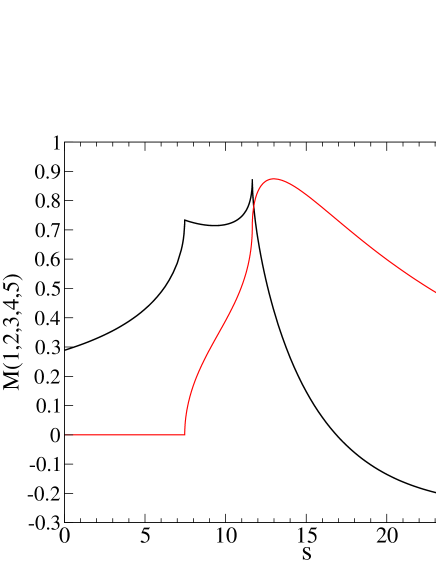
Figure 3: The master integral $M(1,2,3,4,5)$, as a function of $s$. The heavier line is the real part, and the lighter is the imaginary part.

Although the dependence on $s$ near the two-particle thresholds $s=(1+\sqrt{3})^{2}\approx 7.464$ and $(\sqrt{2}+2)^{2}\approx 11.657$ is sharp, these points [and the three-particle thresholds $(1+2+\sqrt{5})^{2}\approx 27.416$ and $(\sqrt{2}+\sqrt{3}+\sqrt{5})^{2}\approx 28.970$] did not present any numerical problems. The value of the master integral at $s=0$ is $[I(1,2,5)-I(1,4,5)-I(2,3,5)+I(3,4,5)]/4\approx 0.28889224$. The asymptotic limit in which equation (6.13) is reasonably accurate is very far to the right of the end of the graph. Values for all of the basis integrals at $s=10$ found from the simultaneous numerical solution to the differential equations are:

$$M(1,2,3,4,5) = \phantom{-}0.71833535+0.39016220i$$

$$U(1,3,4,5) = -4.85695306-2.12756034i$$

$$U(3,1,2,5) = -3.99263620-1.79951451i$$

$$U(2,4,3,5) = -3.08641797$$

$$U(4,2,1,5) = -2.23235894$$

$$S(1,4,5) = -9.56660679$$

$$T(4,1,5) = -0.03036018$$

$$T(5,1,4) = \phantom{-}0.51591658$$

$$T(1,4,5) = -3.01221172$$

$$S(5,2,3) = -7.67047979$$

$$T(5,2,3) = \phantom{-}0.44677524$$

$$T(2,3,5) = -1.69451693$$

$$T(3,2,5) = -0.78612788$$

$$B(1,3) = \phantom{-}0.77930384+1.53905980i\phantom{xxx}$$

$$B(2,4) = -0.05151328\>.$$ (7.2)

As a second test case, consider the master integral $M(x,0,0,x,x)$, which occurs in QED and QCD. This case does not satisfy the criterion for solvability in terms of generalized polylogarithms mentioned in the introduction, but a simple integral representation has been worked out in Broadhurst:1987ei . Following the method adopted here, the full system of differential equations simplifies to:

$$s\frac{d}{ds}B(0,x) = \frac{x}{s-x}\left[B(0,x)+\overline{\rm ln}x-1-s/x\right]\!,\phantom{xxx}$$ (7.3)

$$s\frac{d}{ds}S(0,0,x) = xT(x,0,0)+S(0,0,x)-x\overline{\rm ln}x$$ (7.4)

$$+2x-s/2,$$

$$s\frac{d}{ds}S(x,x,x) = 3xT(x,x,x)+S(x,x,x)-3x\overline{\rm ln}x$$ (7.5)

$$+6x-s/2,$$

$$s\frac{d}{ds}\overline{T}(0,0,x) = \frac{1}{(s-x)^{2}}\bigl{[}x(s-x)\overline{T}(0,0,x)+x(3s+x)T(x,0,0)+2(s+x)S(0,0,x)+x(s-3x)\overline{\rm ln}x$$ (7.6)

$$+5x^{2}+3sx/4-9s^{2}/4\bigr{]},$$

$$s\frac{d}{ds}T(x,0,0) = \frac{1}{s-x}\bigl{[}2xT(x,0,0)+2S(0,0,x)+(s-2x)\overline{\rm ln}x+4x-9s/4\bigr{]},$$ (7.7)

$$s\frac{d}{ds}T(x,x,x) = \frac{1}{(s-x)(s-9x)}\bigl{[}2x(5s-9x)T(x,x,x)+2(s-3x)S(x,x,x)-2sx{\overline{\rm ln}}^{2}x$$ (7.8)

$$+(s^{2}-5sx+18x^{2})\overline{\rm ln}x-36x^{2}+67sx/4-9s^{2}/4\bigr{]},$$

$$s\frac{d}{ds}U(x,0,x,x) = \frac{1}{(s-x)^{2}}\bigl{[}x(s-x)U(x,0,x,x)-x(5s+3x)T(x,x,x)-2(s+x)S(x,x,x)$$ (7.9)

$$+(s+x)x(7\overline{\rm ln}x-{\overline{\rm ln}}^{2}x-11)+s(s+x)/4\bigr{]},$$

$$s\frac{d}{ds}U(0,x,x,0) = \frac{1}{s-x}\bigl{[}xU(0,x,x,0)-xT(x,0,0)-2S(0,0,x)+x(5\overline{\rm ln}x-{\overline{\rm ln}}^{2}x-7)+s/4\bigr{]},$$ (7.10)

$$\frac{d}{ds}[sM(x,0,0,x,x)] = \frac{1}{(s-x)^{2}}\bigl{[}(s+3x)T(x,x,x)+(s+x)T(x,0,0)+2S(x,x,x)+2S(0,0,x)+sB(0,x)^{2}$$ (7.11)

$$+(2\overline{\rm ln}x-4)sB(0,x)+2x(\overline{\rm ln}x-3)^{2}-3s/2\bigr{]}.$$

The value of the master integral obtained for $x=1$ and as a function of $s$ is shown in Figure 4.

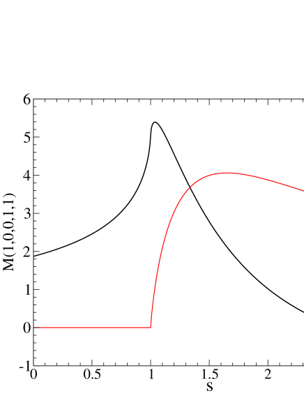
Figure 4: The master integral $M(1,0,0,1,1)$, as a function of $s$. The heavier line is the real part, and the lighter is the imaginary part.

In this example, it turns out that there are numerical problems, but only extremely close to the double threshold at $s=x=1$, where it is known that Broadhurst:1987ei

$$M(1,0,0,1,1)=\pi^{2}\ln 2-3\zeta(3)/2\approx 5.03800311.\phantom{xx}$$ (7.12)

In mass-independent renormalization schemes, this is not an issue since the tree-level mass appearing as the argument of the function is not exactly the same as the pole mass where one will need to evaluate the self-energy. In on-shell type schemes, one could find the threshold value analytically, but one can also use the following general procedure to find threshold values with high accuracy. Near each threshold $s_{0}$, the loop functions have expansions of the form

$$F(s) = F(s_{0})+r[a_{1}+b_{1}\ln r+c_{1}\ln^{2}r]$$ (7.13)

$$+r^{2}[a_{2}+b_{2}\ln r+c_{2}\ln^{2}r]+\ldots$$

where $r=1-s/s_{0}$. Now one can use the Runge-Kutta method to evaluate the loop functions at, say, several points $s=s_{0}\pm n\delta$ (for small integers $n$), and then simply solve for the coefficients in the expansion, in particular $F(s_{0})$. In the present example, I find that choosing $\delta=10^{-4}$, where there are definitely no numerical problems, and $n=1,2,3,4$ is good enough to obtain the threshold values for $s=x=Q=1$ to better than 9 significant digits. The results are:

$$B(0,1) = \phantom{-}2.00000000$$

$$S(0,0,1) = -3.66486813$$

$$T(1,0,0) = \phantom{-}2.78986813$$

$$\overline{T}(0,0,1) = -3.78986813$$

$$U(0,1,1,0) = \phantom{-}2.21013187$$

$$M(1,0,0,1,1) = \phantom{-}5.03800311$$

$$S(1,1,1) = -4.37500000$$

$$T(1,1,1) = -0.50000000$$

$$U(1,0,1,1) = -1.07973627\>.$$ (7.14)

Of these, the first six are checked using the analytic formulas (6.4), (6.16), (6.17), (6.19), (6.20), and (7.12), while the next two can now be seen “experimentally” to have the analytical values $S(1,1,1)=-35/8$ and $T(1,1,1)=-1/2$ at threshold.

To be extra-safe, a computer code can be configured to always trap the threshold and pseudo-threshold cases for evaluation in this manner. This is easy to do in an automated way, since the potentially dangerous points are always known in advance as the roots of the denominators of the differential equations or from inspection of the Feynman diagrams.

VIII Outlook

In this paper I have studied the properties of a minimal basis of integral functions for two-loop self energies. These results include a complete set of formulas allowing for their automated numerical computation using differential equations, following the same strategy as was put forward in Caffo:1998du -Caffo:2002wm . It might be useful to review some of the advantages of this method:

• The basis integrals can be computed for any values of all masses and $s$, to arbitrary accuracy.

• All of the necessary basis integrals are obtained simultaneously in a single numerical computation.

• Branch cuts are automatically dealt with correctly by choosing a contour in the upper-half complex $s$ plane.

• Simple checks on the numerical accuracy follow from changing the choice of contour.

The Tarasov recurrence relation algorithm Tarasov:1997kx ; Mertig:1998vk can be used to reduce any two-loop self-energy to linear combinations of these functions, with coefficients depending on the masses and couplings of the theory. Recently, I have used this basis and the methods of computation described here to obtain the leading two-loop momentum-dependent corrections to the neutral Higgs boson masses in minimal supersymmetry in a mass-independent renormalization scheme. That result will appear soon.

This work was supported by the National Science Foundation under Grant No. 0140129.

References

(1) See for example,
“ATLAS detector and physics performance. Technical design report. Vol. 2,”
CERN-LHCC-99-15,
and V. Drollinger and A. Sopczak,
Eur. Phys. J. C 3, N1 (2001),
hep-ph/0102342.
(2)
For discussions of the present status of the problem,
see
G. Degrassi, S. Heinemeyer, W. Hollik, P. Slavich and G. Weiglein,
Eur. Phys. J. C 28, 133 (2003)
hep-ph/0212020;
S. P. Martin,
Phys. Rev. D 66, 096001 (2002),
hep-ph/0206136 and
Phys. Rev. D 67, 095012 (2003),
hep-ph/0211366.
(3)
O. V. Tarasov,
Nucl. Phys. B 502, 455 (1997)
hep-ph/9703319.
(4)
G. Weiglein, R. Scharf and M. Bohm,
Nucl. Phys. B 416, 606 (1994) hep-ph/9310358.
(5)
A. Ghinculov and Y. P. Yao,
Nucl. Phys. B 516, 385 (1998) hep-ph/9702266;
Phys. Rev. D 63, 054510 (2001)
hep-ph/0006314.
(6)
F. V. Tkachov,
Phys. Lett. B 100 (1981) 65.
K. G. Chetyrkin and F. V. Tkachov,
Nucl. Phys. B 192 (1981) 159.
(7)
O. V. Tarasov,
Phys. Rev. D 54, 6479 (1996) hep-th/9606018.
(8) R. Scharf, Würzburg Diploma Thesis,
as quoted in Scharf:1993ds .
(9)
J.L. Rosner, Ann. Phys. 44, 11 (1967).
(10)
J. van der Bij and M. J. Veltman,
Nucl. Phys. B 231, 205 (1984).
(11)
D. J. Broadhurst,
Z. Phys. C 47, 115 (1990).
(12)
A. Djouadi,
Nuovo Cim. A 100, 357 (1988).
(13)
B. A. Kniehl,
Nucl. Phys. B 347, 86 (1990).
(14)
N. Gray, D. J. Broadhurst, W. Grafe and K. Schilcher,
Z. Phys. C 48, 673 (1990).
(15)
C. Ford and D.R.T. Jones,
Phys. Lett. B 274, 409 (1992).
(16)
C. Ford, I. Jack and D.R.T. Jones,
Nucl. Phys. B 387, 373 (1992)
hep-ph/0111190.
(17)
R. Scharf and J. B. Tausk,
Nucl. Phys. B 412, 523 (1994).
(18)
F. A. Berends and J. B. Tausk,
Nucl. Phys. B 421, 456 (1994).
(19)
J. Fleischer, A. V. Kotikov and O. L. Veretin,
Nucl. Phys. B 547, 343 (1999)
hep-ph/9808242.
(20)
S.P. Martin,
Phys. Rev. D 65, 116003 (2002) hep-ph/0111209.
(21)
V. A. Smirnov,
Commun. Math. Phys. 134, 109 (1990).
(22)
A. I. Davydychev and J. B. Tausk,
Nucl. Phys. B 397, 123 (1993).
(23)
D. J. Broadhurst, J. Fleischer and O. V. Tarasov,
Z. Phys. C 60, 287 (1993)
hep-ph/9304303.
(24)
A. I. Davydychev, V. A. Smirnov and J. B. Tausk,
Nucl. Phys. B 410, 325 (1993)
hep-ph/9307371.
(25)
F. A. Berends, A. I. Davydychev, V. A. Smirnov and J. B. Tausk,
Nucl. Phys. B 439, 536 (1995)
hep-ph/9410232.
(26)
F. A. Berends, A. I. Davydychev and V. A. Smirnov,
Nucl. Phys. B 478, 59 (1996)
hep-ph/9602396.
(27)
A. Czarnecki and V. A. Smirnov,
Phys. Lett. B 394, 211 (1997)
hep-ph/9608407.
(28)
M. Beneke and V. A. Smirnov,
Nucl. Phys. B 522, 321 (1998)
hep-ph/9711391.
(29)
F. A. Berends, A. I. Davydychev and N. I. Ussyukina,
Phys. Lett. B 426, 95 (1998)
hep-ph/9712209.
(30)
A. I. Davydychev and V. A. Smirnov,
Nucl. Phys. B 554, 391 (1999)
hep-ph/9903328.
(31)
J. Fleischer, M. Y. Kalmykov and A. V. Kotikov,
Phys. Lett. B 462, 169 (1999)
hep-ph/9905249.
(32)
M. Caffo, H. Czyz and E. Remiddi,
Nucl. Phys. B 581, 274 (2000)
hep-ph/9912501,
Nucl. Phys. B 611, 503 (2001)
hep-ph/0103014.
(33)
S. Groote and A. A. Pivovarov,
Nucl. Phys. B 580, 459 (2000)
hep-ph/0003115.
(34)
D. Kreimer,
Phys. Lett. B 273, 277 (1991).
(35)
F. A. Berends, M. Buza, M. Bohm and R. Scharf,
Z. Phys. C 63, 227 (1994).
(36)
A. Ghinculov and J. J. van der Bij,
Nucl. Phys. B 436, 30 (1995)
hep-ph/9405418.
(37)
A. Czarnecki, U. Kilian and D. Kreimer,
Nucl. Phys. B 433, 259 (1995)
hep-ph/9405423.
(38)
S. Bauberger, F. A. Berends, M. Bohm and M. Buza,
Nucl. Phys. B 434, 383 (1995)
hep-ph/9409388.
(39)
S. Bauberger, M. Bohm, G. Weiglein, F. A. Berends and M. Buza,
Nucl. Phys. Proc. Suppl. 37B, 95 (1994)
hep-ph/9406404.
(40)
S. Bauberger and M. Bohm,
Nucl. Phys. B 445, 25 (1995)
hep-ph/9501201].
(41)
G. Passarino,
Nucl. Phys. B 619, 257 (2001)
hep-ph/0108252.
(42)
A. V. Kotikov,
Phys. Lett. B 254, 158 (1991).
(43)
A. V. Kotikov,
Phys. Lett. B 259, 314 (1991).
(44)
E. Remiddi,
Nuovo Cim. A 110, 1435 (1997)
hep-th/9711188.
(45)
M. Caffo, H. Czyz, S. Laporta and E. Remiddi,
Nuovo Cim. A 111, 365 (1998)
hep-th/9805118.
(46)
M. Caffo, H. Czyz, S. Laporta and E. Remiddi,
Acta Phys. Polon. B 29, 2627 (1998)
hep-th/9807119.
(47)
M. Caffo, H. Czyz and E. Remiddi,
Nucl. Phys. B 634, 309 (2002) hep-ph/0203256.
(48)
M. Caffo, H. Czyz and E. Remiddi,
“Numerical evaluation of master integrals from differential equations,”
hep-ph/0211178, talk given at RADCOR 2002.
(49)
R. Mertig and R. Scharf,
Comput. Phys. Commun. 111, 265 (1998)
hep-ph/9801383.
(50) L. Lewin, “Polylogarithms and associated functions”
(Elsevier North Holland, New York, 1981).
(51)
K. S. Kolbig,
SIAM J. Math. Anal. 17, 1232 (1986).
(52)
G. ’t Hooft and M. J. Veltman, Nucl. Phys. B 44, 189 (1972);
W. A. Bardeen, A. J. Buras, D. W. Duke and T. Muta,
Phys. Rev. D 18, 3998 (1978).
(53)
W. Siegel,
Phys. Lett. B 84, 193 (1979);
D. M. Capper, D.R.T. Jones and P. van Nieuwenhuizen,
Nucl. Phys. B 167, 479 (1980).
(54)
I. Jack et al,
Phys. Rev. D 50, 5481 (1994)
[hep-ph/9407291].
(55)
G. Passarino and M. J. Veltman,
Nucl. Phys. B 160, 151 (1979).