W and Higgs particle distributions during electroweak tachyonic preheating

Abstract:

We study out-of-equilibrium quasi-particle distributions of the Higgs and W fields during the zero-temperature tachyonic electroweak transition that has been assumed in recent scenarios of baryogenesis. Approximating the process by a fast quench, we perform classical real-time lattice simulations in the SU(2)-Higgs model. The emerging quasi-particle numbers and energies are then used to determine the effective temperatures, chemical potentials and masses of the particles shortly after the transition.

1 Introduction

An electroweak transition, in which the particles of the Standard Model acquired their masses, is assumed to have taken place in the early universe. According to the standard lore, it was a finite-temperature transition. However, in recent scenarios of electroweak baryogenesis [1, 2], this transition is assumed to have taken place at essentially zero temperature shortly after low-scale inflation [3] by the effective mass-squared parameter of the Higgs field going negative (‘tachyonic’) [4, 5, 6, 7]. The resulting spinodal instability has been shown to provide an effective mechanism of preheating [8, 9, 10, 11, 12].

These are topics of non-equilibrium field theory. Quantum fields that are way out of equilibrium need to be treated non-perturbatively, which is well-known to be a difficult task. When applicable, classical approximations can be very useful, since they can be treated by numerical simulation. The tachyonic electroweak transition is an excellent example, since the classical approximation is well justified [5, 6].

Whereas results so obtained are within the language of classical fields, it is desirable to connect with the terminology of kinetic theory, when appropriate. Particle-distribution functions have intuitive appeal; they may be describable by time-depend- ent effective temperatures and chemical potentials. In this paper we address the problem of extracting particle-distribution functions from field-correlation functions obtained in classical approximations.

As is well known, the identification of quasi-particle distributions in field theory is not unique. We use a method that was introduced in [13] for fermions and [14] for bosons. This method has also been found useful in other out-of-equilibrium studies [15, 16, 17, 18, 19, 20, 21], and in QCD studies using the classical approximation applied to the initial stage of heavy-ion collisions [22, 23, 24].

An important topic in electroweak baryogenesis is the time needed for the system to reach approximate thermalization after the transition, and the value of the corresponding effective temperature. The thermalization should be fast enough and the temperature low enough to prevent a possible washout of the generated baryon asymmetry by sphaleron transtions. One of the results in this paper is an estimate of this effective-thermalization time and temperature. However, we shall also find that a temperature is not sufficient to characterize the particle distribution and that a substantial chemical potential is needed as well. A preliminary application to the present case is in [25].

In section 2 we introduce the equations of motion and recall the initial conditions for the tachyonic electroweak quenching transition [5]. Section 3 deals with the definition of distribution functions for the Higgs and W particles, with more details in the Appendix. In section 4 we present results of numerical simulations: particle numbers and effective energies and the determination of effective temperatures and chemical potentials. A discussion of the results is in section 5.

2 Tachyonic electroweak transition

In a tachyonic electroweak transition the effective mass-squared parameter of the Higgs field in the effective potential is assumed to change sign from positive to negative. In hybrid inflation models [4, 7], this is caused by the coupling of the Higgs field to the inflaton field. In a first exploration we assume the transition to be dominated by the dynamics of the SU(2) gauge-Higgs sector of the Standard Model, and model the transition by a quench. At the electroweak energy scale the expansion rate of the universe ($O(10^{-5})$ eV) is negligible compared to the dynamical time scales of the fields and the process can be studied in Minkowski space-time.

2.1 Equations of motion

The SU(2)-Higgs model is given by the action

$$S_{cl}=-\int d^{4}x\left[\frac{1}{2g^{2}}\mbox{Tr}\,F_{\mu\nu}F^{\mu\nu}+(D_{\mu}\phi)^{\dagger}D^{\mu}\phi-\mu^{2}\phi^{\dagger}\phi+\lambda(\phi^{\dagger}\phi)^{2}\right]\,,$$ (1)

with $F_{\mu\nu}=\partial_{\mu}A_{\nu}-\partial_{\nu}A_{\mu}-i[A_{\mu},A_{\nu}]$, $D_{\mu}\phi=(\partial_{\mu}-iA_{\mu})\phi$. Furthermore, $A_{\mu}=A_{\mu}^{a}\tau^{a}/2$, the $\tau^{a}$, $a=1,2,3$ are the Pauli matrices and $\phi$ is the Higgs doublet (our metric is $\mbox{diag}(-1,1,1,1)$). The zero-temperature Higgs and W masses are given by $m_{H}^{2}=2\lambda v^{2}=2\mu^{2}$, $m_{W}^{2}=g^{2}v^{2}/4$, with $v=\mu/\sqrt{\lambda}$ the vacuum expectation value of the Higgs field. The equations of motion are ($m,n=1,2,3$):

$$\partial^{2}_{0}\phi = D_{n}D_{n}\phi+\mu^{2}\phi-2\lambda(\phi^{\dagger}\phi)\phi,$$ (2)

$$\partial_{0}E_{n}^{a} = D_{m}^{ab}F_{mn}^{b}+\frac{ig^{2}}{2}[(D_{n}\phi)^{\dagger}\tau^{a}\phi-\phi^{\dagger}\tau^{a}D_{n}\phi],$$ (3)

with $E^{a}_{n}=F^{a}_{n0}$, $D^{ab}_{n}$ the covariant derivative in the adjoint representation and we have chosen the temporal gauge, $A_{0}=0$. The equations of motion for $A^{a}_{0}$ constitute the three Gauss-constraint equations, which are to be satisfied by the initial conditions. They are conserved by the equations of motion, and read

$$D_{n}^{ab}E_{n}^{b}=\frac{ig^{2}}{2}(\partial_{0}\phi^{\dagger}\tau^{a}\phi-\phi^{\dagger}\tau^{a}\partial_{0}\phi).$$ (4)

For the numerical simulations the action is discretized on a space-time lattice, which leads to discretized equations of motion, see e.g. [26]. More details are given in [27].

2.2 Initial conditions

Before the electroweak transition the system is assumed to be in the symmetric phase ($\langle\phi\rangle=0$) corresponding to an effective action in which the term $-\mu^{2}\phi^{\dagger}\phi$ in (1) is replaced by $\mu^{2}_{\rm eff}\phi^{\dagger}\phi$, with positive $\mu^{2}_{\rm eff}$. The transition is then caused by $\mu^{2}_{\rm eff}$ going through zero and ending up at today’s value $-\mu^{2}$. We model this process by a quench, in which $\mu^{2}_{\rm eff}$ has magnitude $\mu^{2}$ and flips its sign instantaneously: $\mu^{2}_{\rm eff}=\mu^{2}\to-\mu^{2}$. This approximation gives maximal out-of-equilibrium conditions, which we use for testing the baryogenesis scenario [5, 27]. The more gradual transition expected from the coupling to the inflaton field gives qualitatively similar results [6, 7].

The state just after the quench is unstable (the spinodal instability), and in the limit $\lambda\rightarrow 0$, $g^{2}\rightarrow 0$ it is possible to solve exactly the time evolution of the momentum modes of the Higgs field

$$\phi({\bf k},t)=\frac{1}{\sqrt{L^{3}}}\int d^{3}x\,e^{-i{\bf k}\cdot{\bf x}}\,\phi({\bf x},t).$$ (5)

Here $L^{3}$ is the volume of our system with periodic boundary conditions.

The low momentum modes ($|{\bf k}|<\mu$) initially grow roughly exponentially until the interaction terms in the equations of motion become important. Before that happens, the exponential growth leads to large occupation numbers and to effectively sharp values of both canonical variables $\phi$ and $\pi=\partial_{0}\phi$, which justifies the subsequent use of the classical approximation [28, 5, 6]. The full nonlinear back-reaction is thus taken into account without further approximation. This classical approximation should be reasonable for observables that are dominated by the low momentum modes, until classical equipartition sets in, which, as we shall see, does not occur on the time scale of our simulation.

In [5] it was shown that a consistent way to initialize the Higgs field (in the initially free-field approximation), is to generate classical realizations of an ensemble that reproduces the quantum vacuum correlators in the symmetric phase before the quench, i.e.

$$\langle\phi({\bf k})\phi({\bf k})^{\dagger}\rangle=\frac{1}{2\sqrt{\mu^{2}+{\bf k}^{2}}},\qquad\langle\pi({\bf k})\pi({\bf k})^{\dagger}\rangle=\frac{\sqrt{\mu^{2}+{\bf k}^{2}}}{2}.$$ (6)

However, we only initialize the unstable (low momentum $k<\mu$) modes ($k\equiv|{\bf k}|$). This initial condition scheme is the “Just the half” case of [5].

There is an issue concerning how to choose these initial realizations such that they obey the global Gauss law. This technical point is treated in Appendix A of our paper [27] and, for the case of 1+1 dimensions, in [5]. Given a realization of the Higgs field with zero total isospin charges, we can solve the local Gauss-law equations (4) to find the $E_{i}^{a}$. We set $A_{i}^{a}=0$ initially.

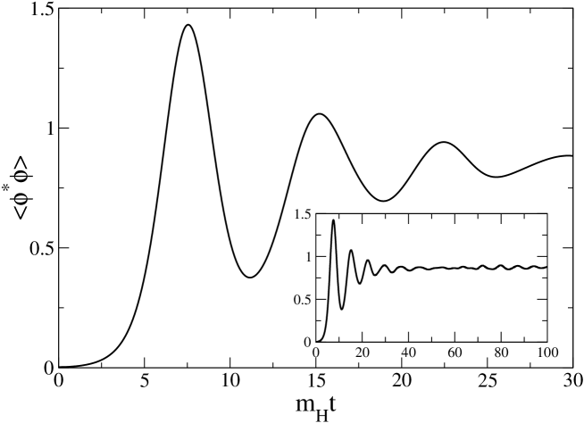
Figure 1: Higgs field expectation values $\langle\phi^{\dagger}\phi\rangle/v^{2}$ versus time. Inset: the long time behavior.

Because only the modes with $k<\mu$ are initialized, we do not expect problems with lattice artifacts until the system equilibrates classically. We will see that this happens on timescales much longer than the ones reached in our simulations (see also [25, 29]).

3 Distribution functions

Under appropriate circumstances kinetic equations can be derived in field theory, in which particle numbers constitute a reduced set of dynamical variables, see, e.g. [30] for the case of QCD. Here we are not concerned with this role of distribution functions, since the dynamics is treated numerically, but consider them as observables for studying the preheating process after the quench.

For interacting fields out of equilibrium the definition of local particle numbers is not unique. At finite (and typically short) times it is not possible to ‘go on shell’, and there may be damping and finite-width effects. However, the system may display effective particle-like behavior in the two-point correlation functions.

In non-abelian gauge theories there is also the question of gauge invariance when the chosen two-point functions are not gauge invariant, as is usually the case. One may render them gauge invariant by supplying parallel transporters along suitable paths, as advocated in [30]. This introduces path-dependence. More generally, there may be field dependence: different fields with the same quantum numbers have different correlators and the resulting particle numbers may or may not depend on the choice being made.

Part of the ambiguities reside in the identification of effective-particle energies, the dispersion relations. We use a method [13, 14] in which the effective-particle numbers and energies are determined selfconsistently. Ref. [13] also contains a study of the effect of using parallel transporters and makes a comparison with the Wigner-function approach. See also [21] for further details on the fermionic case and the relation with conserved charges.

3.1 Higgs and W particle numbers and effective energies

We are interested in the Higgs- and W-quasi-particle distributions, which can be obtained from the $\phi$- and $A$-correlation functions in a suitable gauge. The natural choice of gauge for the Higgs fields is the unitary gauge, in which $\phi$ has only one non-zero real component. For the gauge fields, we will study the particle distribution in both the unitary gauge and in the Coulomb gauge $\partial_{i}A_{i}=0$.

Writing the Higgs field in the form

$$\phi({\bf x},t)=\frac{1}{\sqrt{2}}\begin{pmatrix}\varphi_{2}({\bf x},t)+i\varphi_{1}({\bf x},t)\\ \varphi_{4}({\bf x},t)-i\varphi_{3}({\bf x},t)\end{pmatrix}$$ (7)

where $\varphi_{\alpha}$, $\alpha=1,\cdots,4$ are real, the unitary gauge is defined by

$$\varphi_{a}=0,\;\;\;\;a=1,2,3,\;\;\;\;h\equiv\varphi_{4}>0.$$ (8)

Accordingly, $h=\sqrt{2\phi^{\dagger}\phi}$. The normalization of the fields is chosen such that, in the small amplitude approximation around a ground state, the fields enter in the kinetic part of the (in general effective) action with the canonical normalization. In the present case we have $S=\int d^{4}x\,(1/2)\partial_{0}h\partial_{0}h+\cdots$. After extraction of the gauge coupling $g$, $A^{a}_{n}\to gA^{a}_{n}$, the field $A_{n}^{a}$ is also properly normalized. This normalization criterion can also be applied to composite fields, e.g. the rho-meson field in QCD, provided their effective-action approximation is known.

For simplicity, let us first neglect the coarse graining that is implicit to the notion of distribution functions, and come back to this later. The particle numbers and energies are defined [13, 14] by analogy with the free-field expectation values of the equal-time correlators $\langle\phi\phi\rangle$, $\langle\pi\pi\rangle$, $\langle AA\rangle$, $\langle EE\rangle$ (see also the Appendix). The Higgs particle numbers and effective energies are defined as

$$n^{H}_{k}(t) =\sqrt{\langle h({\bf k},t)h(-{\bf k},t)\rangle_{c}\langle\pi_{h}({\bf k},t)\pi_{h}(-{\bf k},t)\rangle_{c}}\,,$$ (9)

$$\omega^{H}_{k}(t) =\sqrt{\frac{\langle\pi_{h}({\bf k},t)\pi_{h}(-{\bf k},t)\rangle_{c}}{\langle h({\bf k},t)h(-{\bf k},t)\rangle_{c}}}\,,$$ (10)

where $\langle\cdots\rangle_{c}$ is the connected two-point function given by $\langle AB\rangle_{c}\equiv\langle AB\rangle-\langle A\rangle\langle B\rangle$. We have replaced the ‘quantum’ particle-number combination $n_{k}+1/2$ with the ‘classical’ $n_{k}$, and used spherical symmetry to write these as a function of $k=|{\bf k}|$.

In a general gauge, we can decompose the gauge field two-point function in a transverse and a longitudinal part, as

$$\langle A^{a}_{i}({\bf k},t)A^{b}_{j}(-{\bf k},t)\rangle =\delta_{ab}\bigg{[}\Big{(}\delta_{ij}-\frac{k_{i}k_{j}}{k^{2}}\Big{)}D_{T}^{A}(k,t)+\frac{k_{i}k_{j}}{k^{2}}D_{L}^{A}(k,t)\bigg{]}\,,$$ (11)

$$\langle E^{a}_{i}({\bf k},t)E^{b}_{j}(-{\bf k},t)\rangle =\delta_{ab}\bigg{[}\Big{(}\delta_{ij}-\frac{k_{i}k_{j}}{k^{2}}\Big{)}D_{T}^{E}(k,t)+\frac{k_{i}k_{j}}{k^{2}}D_{L}^{E}(k,t)\bigg{]}\,.$$ (12)

The $\delta_{ab}$ reflect the fact that the initial conditions are isospin symmetric. In the Coulomb gauge, the gauge potential is purely transverse, $D_{L}^{A}(k,t)=0$ (but $D_{L}^{E}(k,t)\neq 0$), and the $n^{A}_{k}$ and $\omega^{A}_{k}$ can be defined analogously to the Higgs case:

$$n^{A}_{k}(t)\equiv\sqrt{D^{A}_{T}(k,t)D^{E}_{T}(k,t)}\,,\qquad\omega^{A}_{k}(t)\equiv\sqrt{\frac{D^{E}_{T}(k,t)}{D^{A}_{T}(k,t)}}\,.$$ (13)

In the unitary gauge, the free-field correlators are those of a massive Yang-Mills field (the derivation is given in the Appendix):

$$\langle A_{i}({\bf k},t)A_{j}(-{\bf k},t)\rangle =\Big{(}\delta_{ij}+\frac{k_{i}k_{j}}{m_{W}^{2}}\Big{)}\frac{n_{k}}{\omega_{k}}\,,$$ (14)

$$\langle E_{i}({\bf k},t)E_{j}(-{\bf k},t)\rangle =\Big{(}\delta_{ij}-\frac{k_{i}k_{j}}{k^{2}+m_{W}^{2}}\Big{)}n_{k}\omega_{k}\,.$$ (15)

We decompose this into longitudinal and transverse modes, and arrive at the expressions we will use to determine longitudinal and transverse occupation numbers and mode energies in the unitary gauge,

$$n^{T}_{k} =\sqrt{D^{A}_{T}(k)D^{E}_{T}(k)}\,, \qquad\omega^{T}_{k} =\sqrt{\frac{D^{E}_{T}(k)}{D^{A}_{T}(k)}}\,,$$ (16)

$$n^{L}_{k} =\sqrt{D^{A}_{L}(k)D^{E}_{L}(k)}\,, \qquad\omega^{L}_{k} =m_{\rm eff}^{L2}\sqrt{\frac{D^{A}_{L}(k)}{D^{E}_{L}(k)}}\,.$$ (17)

The transverse case is analogous to the Higgs case. In the longitudinal case we assumed the form $\omega_{k}^{L2}=m_{\rm eff}^{L2}+k^{2}$ and replaced $m_{W}^{2}\to m_{\rm eff}^{L2}$ in (14,15). Then (17) follows straightforwardly. Note the inverse dependence on $D^{E}/D^{A}$ in $\omega^{L}$. In practice we analyze the data by first replacing $m_{\rm eff}^{L}\to m_{W}$ in (17), and then correct for it.

3.2 Coarse graining

Consider the problem of defining a position-dependent distribution function $n({\bf x},{\bf k},t)$ for a system out of spatial equilibrium. A natural approach is to consider a region $R({\bf x})$ of size $B$ around the position ${\bf x}$, e.g. a cube of volume $B^{3}$, and to focus on this region. This means restricting the Fourier integrals etc. in the formulas in the previous section to the region $R({\bf x})$. The size of the region then determines the precision in momenta and positions of the particles. Similarly, one expects to have to do some coarse graining in time in order to control the fluctuations in the energies of the particles. Such time averages were taken in [14, 16], but since we try to follow the out-of-equilibrium process in time as closely as possible, we shall not do so here.

For simplicity, consider a scalar field in 1+1 dimensions and let the localized region $R(x)$ be the interval $(x-B/2,x+B/2)$. The correlators in momentum space associated with $R(x)$ are then given by (suppressing the common time label)

$$C_{\varphi\varphi}(x,k) = \int_{x-B/2}^{x+B/2}dy\,dz\,\frac{e^{-iky+ikz}}{B}\,\langle\varphi(y)\varphi(z)\rangle_{c},$$

$$C_{\pi\pi}(x,k) = \int_{x-B/2}^{x+B/2}dy\,dz\,\frac{e^{-iky+ikz}}{B}\,\langle\pi(y)\pi(z)\rangle_{c},$$ (18)

from which we obtain the distribution functions in the quantum theory as

$$C_{\varphi\varphi}(x,k)=\frac{n(x,k)+1/2}{\omega(x,k)},\;\;\;\;C_{\pi\pi}(x,k)=(n(x,k)+1/2)\,\omega(x,k).$$ (19)

In the classical approximation the ‘1/2’ is left out.

For a homogeneous system we can improve statistics by taking a spatial average,

$$C_{\varphi\varphi}(k) = \frac{1}{L}\int dx\,C_{\varphi\varphi}(x,k)=\sum_{p}w(p-k)\,\langle\varphi(p)\varphi(-p)\rangle,$$ (20)

$$w(p-k) = \frac{4\sin^{2}[(p-k)B/2]}{BL(p-k)^{2}},$$ (21)

and similar for the $\pi\pi$ correlator ($\varphi(p)$ is the Fourier transform in the total volume, as in (5)). The weight function $w(p-k)$ is sharply peaked about $p=k$ and normalized,

$$\sum_{p}w(p-k)=1.$$ (22)

The particle numbers are obtained after the spatial averaging,

$$C_{\varphi\varphi}(k)=\frac{n_{k}+1/2}{\omega_{k}},\;\;\;\;C_{\pi\pi}(k)=(n_{k}+1/2)\,\omega_{k}.$$ (23)

The coarse graining has the effect of smoothing out the correlators in momentum space. This is a welcome feature, since the initial momentum modes of the fields are uncorrelated, no matter how large the volume (their variance is given by (6)).

In practise we implement spatial coarse graining by ‘binning’ our momenta spherically, for example for the Higgs field:

$$\langle h({\bf k},t)h(-{\bf k},t)\rangle\to\frac{1}{N_{k}}\sum_{-k-\Delta<|{\bf p}|<k+\Delta}\langle h({\bf p},t)h(-{\bf p},t)\rangle,$$ (24)

where $N_{k}$ is the number of independent momenta in the momentum bin labelled by $k$. In position space this corresponds to spherical shells of thickness of order $\pi/\Delta$.

3.3 Early time

The exponential growth of the particle numbers after the quench was studied in [5] in the approximation $\lambda=g=0$. For each real mode $\varphi_{\alpha}$, $\alpha=1,\cdots,4$, of the Higgs field, the particle number in the unstable region ($k<\mu$) is given by

$$n_{k}^{\alpha}=\left[\frac{1}{4}+\frac{\mu^{4}}{4(\mu^{4}-k^{4})}\,\sinh^{2}(2\sqrt{\mu^{2}-k^{2}}\,t)\right]^{1/2}-\frac{1}{2}\approx\frac{1}{4}e^{2\sqrt{\mu^{2}-k^{2}}\,t},$$ (25)

where the last form holds for $2\sqrt{\mu^{2}-k^{2}}\,t\gg 1$. The field correlators are given by

$$C_{k}^{\varphi_{\alpha}\varphi_{\beta}}=\delta_{\alpha\beta}\,\frac{1}{2\sqrt{\mu^{2}+k^{2}}}\left[1+\frac{2\mu^{2}}{\mu^{2}-k^{2}}\,\sinh^{2}(\sqrt{\mu^{2}-k^{2}}\,t)\right].$$ (26)

Using the above information we can estimate the particle number at a time $t_{\rm nl}$ where the neglected nonlinearities may be expected to stop the exponential growth. We identify $t_{\rm nl}$ with the time where $\langle\varphi_{\alpha}\varphi_{\alpha}\rangle$ (unstable modes only) reaches the inflexion point $\mu^{2}/3\lambda$ of the Higgs potential, i.e.

$$\langle\varphi_{\alpha}\varphi_{\alpha}\rangle=\sum_{\alpha}\int\frac{d^{3}k}{(2\pi)^{3}}\,C^{\varphi_{\alpha}\varphi_{\alpha}}=\frac{\mu^{2}}{3\lambda}.$$ (27)

For the parameters ($\lambda=1/9$) used in our simulation this gives $t_{\rm nl}=3.32321\,\mu^{-1}$. Then (25) gives for the particle number of each real mode at zero momentum

$$n_{0}^{\alpha}(t_{\rm nl})=193.$$ (28)

The distribution at that time is plotted in figure 2, together with the frequency $\omega_{k}$ [5].

Figure 2: Left: $n_{k}$ for a real Higgs mode versus $k$. Right: $\omega_{k}$ and $\sqrt{|\mu^{2}-k^{2}|}$ versus $k$. The units are $\mu=m_{H}/\sqrt{2}$ and the time is $t=3.32321\,\mu^{-1}=4.7\,m_{H}^{-1}$.

We have not attempted to compute the corresponding quantities for the radial mode $h=\sqrt{\varphi_{\alpha}\varphi_{\alpha}}$, but expect them to be similar.

4 Results

We have performed simulations with $g=2/3$, $\lambda=1/9$, giving $m_{H}^{2}/m_{W}^{2}=2$, and volume $L^{3}=21^{3}\,m_{H}^{-3}$. All results shown will be quoted in units of the zero-temperature Higgs mass $m_{H}$.

We used a $60^{3}$ lattice, with lattice spacing $a=0.35\,m_{H}^{-1}$. The maximum momentum in each direction is $\pi/a=9.0\,m_{H}$, but reasonably accurate continuum behavior is expected to be limited to the region $|k_{i}|<1/a=2.8\,m_{H}$. As is well-known, lattice-artifacts are substantially reduced by using the corrected momentum $k^{\prime}_{i}=(2/a)\sin(ak_{i}/2)$. In the following we always use $k^{\prime}_{i}$ and drop the prime.

We generated 42 independent realizations of the initial conditions (6), and sampled the subsequent time evolution for $tm_{H}=1$, 2, …, 12, 20, 30, 40, 50, 100. The Coulomb-gauge fixing has been performed using an overrelaxation algorithm [31, 32], stopping when $L^{-3}\sum_{{\bf x},a}|\partial_{i}A_{i}^{a}({\bf x})|^{2}<10^{-15}$ in lattice units. This precision has been chosen to ensure that also the low-momentum modes are tranverse to a high degree of accuracy.

We have averaged nearby momenta as described in section 3.2, within ‘bins’ of size $2\Delta=0.05\,a^{-1}=0.0175\,m_{H}$. The zero-mode is always in a bin of its own, and will be treated separately in that it will not be included in any fit to the data.

4.1 Particle distributions

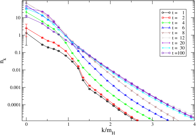
Figure 3: Higgs-particle numbers as a function of $k$.

In figure 3 we show the particle distribution for the Higgs fields. We see that the occupation numbers of the low-momentum modes increases exponentially up to $t\approx 6-8\,m_{H}^{-1}$, where they start saturating to an $n_{0}$ of about 100. At this point, the high-momentum modes rapidly become populated, and after $t\approx 20\,m_{H}^{-1}$ the system evolves only very slowly, resulting in an approximately exponential distribution.

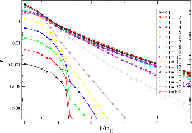
Figure 4: Coulomb-gauge W-particle numbers as a function of $k$.

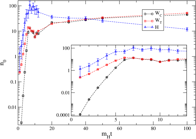
Figure 5: Particle numbers of the zero modes as a function of time; $H$: Higgs; $W_{T}$: transverse W in unitary gauge; $W_{C}$: transverse W in Coulomb gauge; inset: early time.

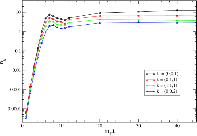
Figure 6: Coulomb-gauge W-particle numbers for the four lowest momentum modes, as a function of time.

In figure 4 we show the Coulomb-gauge W-particle numbers for all times. We see the same qualitative behavior as for the Higgs field, with the occupation numbers increasing exponentially up to $t\approx 6\,m_{H}^{-1}$, where they start saturating to $n_{0}\approx 15$, followed by a rapid growth in the high-momentum modes (‘sudden up-sweep of the tail’) and only a slow evolution for $t\gtrsim 20\,m_{H}^{-1}$. The main difference with the Higgs case is that the initial particle numbers are much lower — initially all the energy is in the Higgs fields. In figure 5 we show the time evolution of the particle numbers $n_{0}$ of the zero modes.

The exponential growth and subsequent slow evolution can also be seen by plotting the lowest non-zero momentum modes separately as a function of time, as in figure 6.

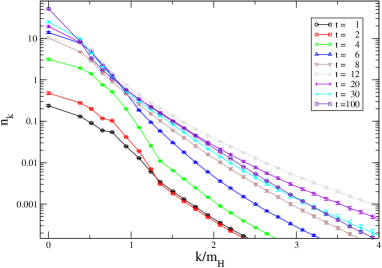
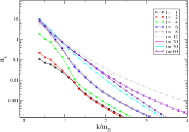
Figure 7: Unitary-gauge transverse (left) and longitudinal (right) W-particle numbers as a function of $k$.

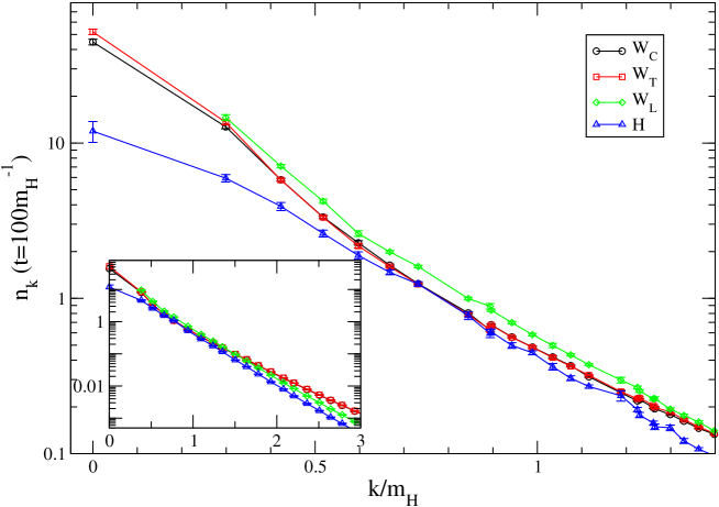
Figure 8: Particle distributions at the latest time, for all four particle ‘species’.

Figure 7 shows the W-particle distribution in the unitary gauge, with the longitudinal and transverse modes plotted separately. Note that the longitudinal zero mode is not defined. The same qualitative behavior as before can be seen. In this case the initial particle numbers are much larger and close to those of the Higgs field, which is natural since the Goldstone modes, which are absorbed into the unitary-gauge W-fields, are also populated by the initial conditions (6).

Finally, in figure 8, we show the particle distribution for all four ‘species’ (Coulomb-gauge W, transverse and longitudinal unitary-gauge W, and Higgs) at the latest time, $t=100\,m_{H}^{-1}$. We see, firstly, that all four have an exponential fall-off at large momenta. Secondly, for $k\lesssim 0.7\,m_{H}$ the occupation number remains significantly above 1, vindicating our use of the classical approximation. Thirdly, the transverse gauge field modes have almost exactly the same distribution in the unitary gauge as in the Coulomb gauge. The distribution of the longitudinal modes on the other hand deviates somewhat from that of the transverse ones.

4.2 Dispersion relation and effective mass

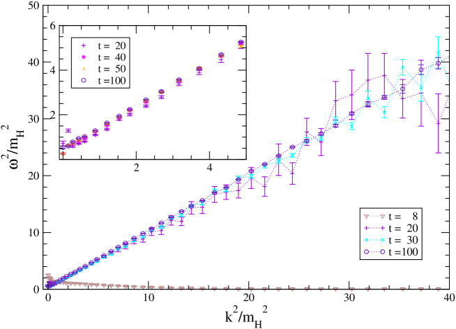
Figure 9: Dispersion relation for W-particles in Coulomb gauge.

In figure 9 we show the dispersion relation, $\omega^{2}$ as a function of $k^{2}$, for Coulomb-gauge W-particles. For $t\lesssim 20\,m_{H}^{-1}$ there is no sensible dispersion relation, as can be seen from the data for $t=8$; while for $t\gtrsim 30\,m_{H}^{-1}$ it approaches the form $\omega^{2}=m_{\text{eff}}^{2}+ck^{2}$, with $c\approx 1$. The inset shows the dispersion relation for $t=30,40,50$ and $100\,m_{H}^{-1}$ in a more restricted momentum range. The data are very well described by a straight line, and for $t=40,50$ and $100\,m_{H}^{-1}$ they are indistinguishable. It is striking that the data turn out to be compatible with a straight line all the way up to $k^{2}=40m_{H}^{2}$, far into the region where one would expect lattice artifacts to dominate and the classical approximation to break down.

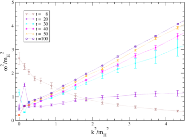
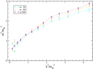
Figure 10: W-particle dispersion relation in the unitary gauge, for transverse (left) and longitudinal (right) modes.

In figure 10 we show the dispersion relation in the unitary gauge. In this case, a particle-like behavior takes considerably longer to emerge than in the Coulomb gauge: for the transverse modes the slope is still smaller than 1 (and increasing) at the latest time, $t=100\,m_{H}^{-1}$, while for the longitudinal modes a curvature remains for $k^{2}>m_{H}^{2}$. However, the intercepts (effective mass-squared) are quite compatible.

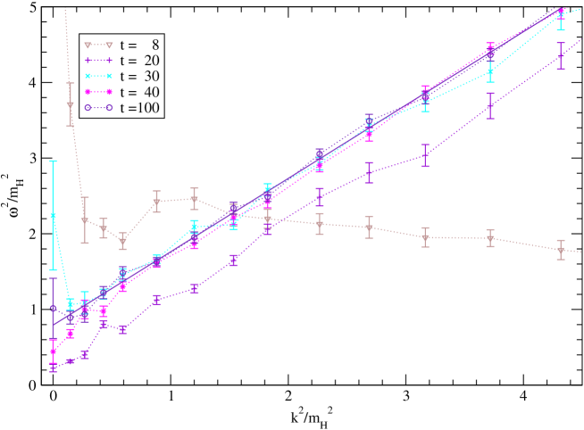
Figure 11: Dispersion relation for Higgs particles. Also shown is the best fit to a straight line for $t=100\,m_{H}^{-1}$.

In figure 11 we show the dispersion relation for the Higgs particles, for $tm_{H}=8$, 20, 30, 40, 100. Here again, we find that the dispersion relation is stable for $t\gtrsim 30\,m_{H}^{-1}$. Evidently, there is still some remnant of the odd-looking dispersion relation $\omega_{k}^{2}\approx|\mu^{2}-k^{2}|$ during exponential growth at early times, shown in figure 2. Standard $\omega_{k}^{2}=m_{\rm eff}^{2}+k^{2}$-like behavior emerges between $tm_{H}=12$ and 20. Note also that the W-dispersion relation at $tm_{H}=8$ in figures 9 and 10 shows similar behavior: the various field modes appear to adjust to each other locally in momentum space. This can also be seen in the particle numbers. Similar ‘local momentum space equilibration’ has been observed and explained in [16].

We fit the effective energies to the form $\omega_{k}^{2}=ck^{2}+m_{\text{eff}}^{2}$. The uncertainty in the dispersion relation is estimated by varying the end-point $k_{\text{max}}$ of the fitting range and determining the statistical errors by the bootstrap method. In figure 12 we show the result of this procedure for the slope of the Higgs dispersion relation.

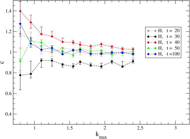
Figure 12: Slope of the dispersion relation for the Higgs field as a function of the maximum momentum in the fit.

We find that in order to obtain stable values for $c$ and $m_{\text{eff}}$, we need to include points up to $k\approx 2\,m_{H}$ in our fits, while beyond this point the fit values do not change significantly. This was the case for all the fits we performed, and we have thus chosen $k_{\text{max}}=2\,m_{H}$ when quoting the fit parameters and statistical errors in table 1.

$t$	$W_{C}$		$W_{T}$		H
	$m_{\text{eff}}$	$c$	$m_{\text{eff}}$	$c$	$m_{\text{eff}}$	$c$
30	0.56(2)	0.94(2)	0.59(3)	0.70(5)	0.93(2)	0.91(3)
40	0.64(1)	0.974(6)	0.67(1)	0.69(3)	0.79(3)	1.02(2)
50	0.66(1)	0.970(7)	0.67(1)	0.79(1)	0.84(2)	1.01(2)
100	0.68(1)	0.972(7)	0.69(1)	0.828(6)	0.89(2)	0.98(2)

Table 1: Effective masses (in $m_{H}$ units) and slopes in the dispersion relation. The errors are purely statistical.

For the gauge fields, the intercepts (effective masses) in the two gauges are compatible, yielding a value $m_{\text{eff}}\approx 0.68\,m_{H}$, close to the zero-temperature value $0.71\,m_{H}$. However, the slope, which in the Coulomb gauge is very close to 1, is considerably lower in the unitary gauge, although it appears to approach 1 with increasing time. Quasi-particle behavior appears to take longer to emerge in this gauge. For the Higgs field, we find an effective mass $\approx 0.88\,m_{H}$ at $t=100\,m_{H}^{-1}$, which is significantly smaller than the zero-temperature Higgs mass, although it appears to be increasing with time. The slope is found to be consistent with 1 from $t=40\,m_{H}^{-1}$ onwards. The effective Higgs mass appears to be increasing with time, which may be expected from the fact that $v_{\rm eff}^{2}\equiv\langle\phi^{\dagger}\phi\rangle$ (averaged over an oscillation period) is still slowly increasing (figure 1). One would expect a component $v_{\rm eff}/v\approx 0.87$ in both effective Higgs and W mass ratios, but the effective W mass somehow seems to have settled from $t=40\,m_{H}^{-1}$ onwards.

Finally we turn to the longitudinal dispersion relation $\omega_{k}^{L}$. In plotting the data in figure 10 (right) we used $m_{W}$ instead of $m_{\rm eff}^{L}$ in eq. (17), and we now consider this point. Let $\omega^{\prime}_{k}$ be the frequency defined by (17) with $m_{\rm eff}^{L}\to m_{W}$. Then $\omega_{k}^{L}=(m_{\rm eff}^{L2}/m_{W}^{2})\omega_{k}^{\prime}$ and $m_{\rm eff}^{L}=(m_{W}^{2}/m^{\prime})$, where $m^{\prime}=\omega^{\prime}_{0}$. The data for $\omega_{k}^{\prime 2}$ with $k^{2}/m_{H}^{2}\lesssim 1$ in figure 10 (right, $tm_{H}=100$) can be fitted well by a straight line with slope very close to 1, and effective mass $m^{\prime 2}\approx 0.49\,m_{H}^{2}\approx m_{W}^{2}$. It follows that $m_{\rm eff}^{L}\approx m_{W}$ to a good approximation.

The different slopes in the dispersion relations may be interpretable by simple parameter changes in an effective quasi-particle lagrangian, but we shall not follow up on this here.

4.3 Approximate thermalization, temperature and chemical potential

We will model the particle distribution with a Bose–Einstein (BE) distribution,

$$n_{k}=\frac{1}{e^{(\omega_{k}-\mu)/T}-1}.$$ (29)

It may seem strange to use the BE form instead of the classical $n_{k}=T/(\omega_{k}-\mu)$, but this form would not be able to describe the roughly exponential tail of the $n_{k}$ data. We use the BE form simply as a distribution to compare the data with, in order to extract effective temperatures and chemical potentials. The BE form may be re-expressed as

$$B_{k}\equiv\ln\Big{(}1+\frac{1}{n_{k}}\Big{)}=\frac{\omega_{k}-\mu}{T}$$ (30)

If we have a Bose–Einstein distribution, $B_{k}$ is a linear function of $\omega_{k}$, and in a plot of $B$ vs $\omega$, the inverse temperature can be read off as the slope. We will therefore refer to such plots as ‘inverse-temperature plots’.

We will use two methods to determine effective temperatures and chemical potentials. The first (method 1) is to perform a straight-line fit to (30), using the data for $n_{k}$ and $\omega_{k}$. The second (method 2) is to take $\omega_{k}$ from the dispersion relation, using the fitted values for $c$ and $m_{\text{eff}}$ determined in the previous section. We then fit $n_{k}$ directly as a function of $\omega_{k}$ to the Bose–Einstein distribution (29).

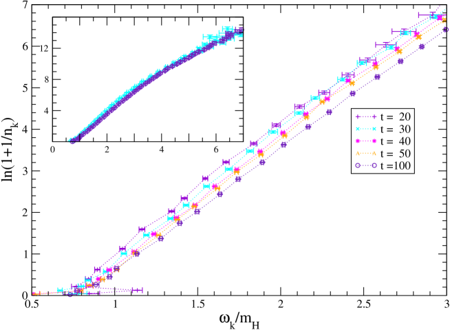
Figure 13: Inverse-temperature plot for W particles in Coulomb gauge.

In figure 13 we show $B$ as a function of $\omega$ for Coulomb-gauge W particles, for $t=20,30,40,50,100\,m_{H}^{-1}$. For $\omega_{k}<2.5-3m_{H}$ the data are compatible with a Bose–Einstein distribution, with a rather large chemical potential. At higher energies, as shown by the inset, there is some curvature around $\omega_{k}=4$. In this region the particle numbers are very small and it is clearly way beyond the range of validity for the classical approximation. It is nevertheless interesting to see that the qualitative behavior of the distribution is unchanged as we go from the infrared to the ultraviolet. We also see that the distribution changes only very slightly with time, with the effective temperature slowly increasing. The same qualitative picture is found also in the unitary gauge.

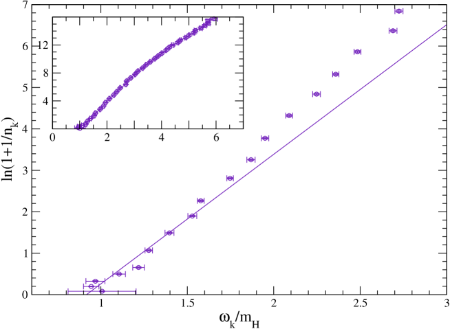
Figure 14: Inverse-temperature plot for Higgs particles for $t=100\,m_{H}^{-1}$. The line is the best fit to a straight line for $\omega_{k}<1.6\,m_{H}$

Figure 14 shows $B$ as a function of $\omega$ for the Higgs fields at the latest time. The statistical errors in $\omega$ are larger here than for the W fields. A fit to a straight line through the lowest modes — those where $n_{k}\gtrsim 1$ — deviates from the data at higher $\omega$, and, as seen in the inset, there is a curvature in the region $\omega_{k}=2.5-4$.

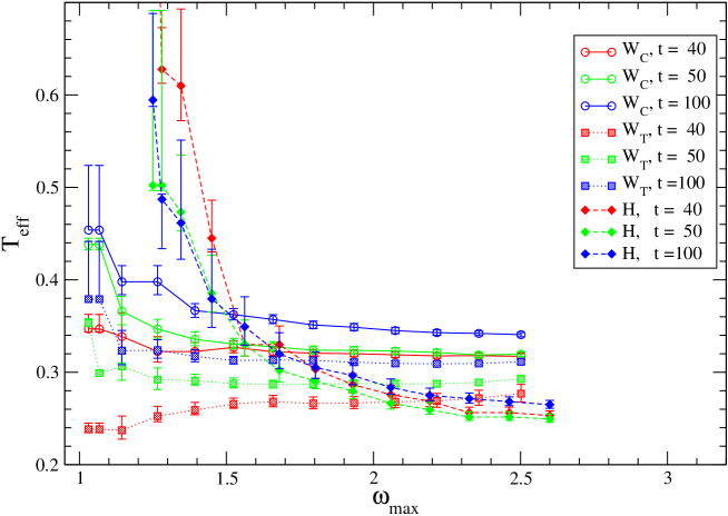
Figure 15: Effective temperature, from inverse-temperature fits, as a function of fitting range.

Figure 15 shows the fitted temperature $T$ from the straight-line fits, as a function of the end-point $\omega_{\text{max}}$ of the fitting range. We have chosen $\omega_{\rm max}=2.1$, which is below the region where $B_{k}$ shows curvature in the inserts in figures 13 and 14.

$t$	$W_{C}$		$W_{T}$		H
	$T_{1}$	$\mu_{1}$	$T_{1}$	$\mu_{1}$	$T_{1}$	$\mu_{1}$
30	0.320(8)	0.717(12)	0.24(4)	0.73(4)	0.23(2)	1.07(3)
40	0.319(3)	0.772(8)	0.268(8)	0.742(9)	0.28(3)	0.94(3)
50	0.323(4)	0.786(9)	0.298(3)	0.758(8)	0.27(2)	0.97(3)
100	0.345(6)	0.786(9)	0.309(4)	0.781(7)	0.28(2)	0.95(3)

Table 2: Effective temperatures and chemical potentials, from fits to $0<\omega<2.1m_{H}$. The quoted errors are a combination of the statistical errors and systematic errors obtained by varying the fit range with $\omega_{\text{max}}$ between 1.6 and $2.6m_{H}$.

The fit values are given in table 2. Since they were obtained with method 1, we have added the subscript 1 to $T_{1}$ and $\mu_{1}$. The effective temperature $T_{1}$ in the unitary gauge turns out to be somewhat lower than in the Coulomb gauge: 0.31 compared to 0.35  $m_{H}$ at the latest time. This can be put down to the slope of the dispersion relation being lower, resulting in a smaller effective energy for the same mode. The chemical potentials are consistent between Coulomb and unitary gauge, giving a value $\mu\approx 0.78\,m_{H}$. This is higher than the effective mass $\approx 0.68\,m_{H}$ in table 1, which is of course nonsensical, since it would lead to a pole in $n_{k}$ for very small $k$. The effective temperature for the Higgs is similar to that of the W fields, although slightly lower $\approx 0.28\,m_{H}$. The chemical potential for the Higgs comes out to be $\approx 0.95\,m_{H}$, again higher than the effective mass $\approx 0.88\,m_{H}$ in table 1.

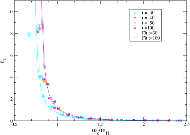
Figure 16: W-particle number at $t=30,40,50,100\,m_{H}^{-1}$ as a function of the effective energy $\omega$, together with the Bose–Einstein distribution (29) with parameters from table 2. The dotted lines indicate the variation allowed by the errors in the fitted $T$ and $\mu$.

Figure 16 shows the Coulomb-gauge W-particle number as a function of the effective energy $\omega$, together with the best inverse-temperature fit to the five lowest-lying modes. These data do not appear to be particularly well described by a Bose–Einstein distribution, largely due to what appears to be a somewhat erratic behavior of the effective energy $\omega_{k}$. Replacing $\omega_{k}$ with values taken from the fits in table 1, we obtain a much smoother data plot, as shown in figure 17.

$t$	$W_{C}$		$W_{T}$		H
	$T_{2}$	$\mu_{2}$	$T_{2}$	$\mu_{2}$	$T_{2}$	$\mu_{2}$
30	0.50(1)	0.62(1)	0.33(3)	0.64(2)	0.45(2)	0.97(2)
40	0.420(7)	0.698(11)	0.31(1)	0.713(10)	0.58(6)	0.83(3)
50	0.427(7)	0.721(9)	0.335(7)	0.719(10)	0.46(2)	0.88(2)
100	0.424(6)	0.735(9)	0.370(5)	0.733(9)	0.38(1)	0.90(2)

Table 3: Effective temperatures and chemical potentials, from fits to the lowest 5 non-zero modes (method 2).

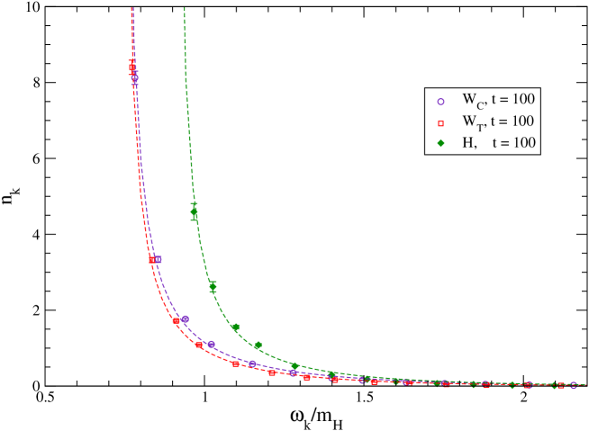
Figure 17: Higgs and W-particle numbers at $t=100\,m_{H}^{-1}$ as a function of the effective energy $\omega$ taken from the fitted dispersion relation. Also shown is the Bose–Einstein distribution (29) with parameters from table 3. The zero-modes are outside the boundaries of the plot (they are given by $(0.68,45(2))$ for $W_{C}$, $(0.69,52(2))$ for $W_{T}$ and $(0.89,12(2))$ for $H$).

We fit the 5 lowest-lying modes (for which $n_{k}\gtrsim 0.5$) of these data to a Bose–Einstein distribution (method 2) and give the results in table 3. The fit describes the displayed data well in the important region where the classical approximation is supposed to be valid.

Again we find that the effective temperature for the W particles in the unitary gauge is lower than in Coulomb gauge, due to the lower slope of the dispersion relation. On the other hand, the effective Higgs-temperature is falling from $t=40\,m_{H}^{-1}$ onwards and the unitary-gauge W-temperature is rising. A conversion of energy in the Higgs to the W may still be going on at the latest time, which is also suggested by the behavior of the zero modes in figure 5.

The chemical potentials both for the Higgs and W particles are lower than those obtained using method 1, reflecting the fact that modes with small $\omega$ have a larger weight. For the Higgs, $\mu_{2}$ is compatible with the effective mass, but for the W it is still larger. Note that the zero-modes have not been included in any of the fits. It turns out that they have occupation numbers much lower than would be ‘predicted’ by any Bose–Einstein distribution that would simultaneously fit the other ‘classical’ modes.

This is another indication (in addition to chemical potentials larger than effective masses) that the BE fit will overestimate the true distribution for momenta below our lowest finite-volume momentum $k_{\rm min}=2\pi/L=0.30\,m_{H}$. The flattening of the distribution in figure 2 as $k\to 0$ appears to be very resilient.

5 Conclusions

We have obtained Higgs- and W-particle distributions and energies after a quenched electroweak transition, when the system is still out of equilibrium, for the case $m_{H}=\sqrt{2}\,m_{W}$. The particle distributions could be obtained from early times $t=1/m_{H}$ onwards. On the other hand, the effective energies (frequencies) suffered much more from fluctuations and they appeared to get conventional forms only after $t\gtrsim 20\,m_{H}^{-1}$. Much more statistics would be required to go determine them with reasonable accuracy at earlier times (where they retain the memory of the instability). The Coulomb-gauge W distribution appears to be smoother than the corresponding transverse distribution in the unitary gauge, but the two approach each other and by the time $100\,m_{H}^{-1}$ they are practically indistinguishable. At this stage the gauge dependence has practically disappeared; also the longitudinal W modes have settled to nearly the same distribution. We have carried out a few simulations up to times $500\,m_{H}^{-1}$, which showed that the distributions change very slowly after time $100\,m_{H}^{-1}$.

The maximum value of the Higgs-particle number turned out to be smaller than the analytical estimate in (28), by a factor of $2$. This mismatch is evidently due to the fact that with the “Just a half” initial conditions, the interactions (including the Coulomb interaction generated by the Gauss constraint) are turned on straight away from time zero onwards, and that the driving power of the instability is damped by sharing energy with the gauge field. At low momenta the particle numbers are still large even at $t=100\,m_{H}^{-1}$ and there is no reason to doubt the classical approximation for these modes. In contrast, the high-momentum modes are still exponentially suppressed at this time and there is no sign yet of classical equipartition ($n_{k}\propto 1/k$ for large $k$) in our simulation. Hence, lattice artifacts are expected to be small in the low-momentum part of the distributions.

Although we know of no good reason to expect a Bose–Einstein distribution, this form fitted the data quite well in the important (low momentum) region (figure 17). The same is true at intermediate momenta, where the particle numbers are much smaller than one, albeit with slightly different temperature and chemical potential. This is fortunate, since it allows for a familiar interpretation of the results. The final temperatures of the Higgs and W degrees of freedom turned out to be reasonably close at time $100\,m_{H}^{-1}$, which indicates that the system is near kinetic equilibrium. In contrast, the rather large chemical potentials show that it is still far from chemical equilibrium. For very low momenta (lower than our finite-volume simulation was able to deal with) the BE fit has to break down because the chemical potentials are slightly larger than the effective masses.

The temperature in the gauge fields at time $100\,m_{H}^{-1}$ is relatively low, $0.44\,m_{H}$, which suggest that sphaleron transitions are highly suppressed. However, such a conclusion cannot be drawn from the temperature alone. The large chemical potentials correspond to the fact that there is still quite some power in the low momentum modes, and sphaleron transitions might still be non-negligible over a long time span. However, in the full Standard Model the Higgs and W particles will have decayed in a few hundred $\,m_{H}^{-1}$ and we do not see a problem with the baryogenesis scenario.

Appendix A Free-field correlators in Higgs and Coulomb gauge

We derive here the free-field correlators used for guidance in the definition of the distribution functions in the unitary gauge and the Coulomb gauge.

In the unitary gauge, expanding around the ground-state configuration $h=v$, $A_{\mu}^{a}=0$, and keeping only terms up to second order in the fields, leads to the effective free-field lagrangian

$$L_{\rm free} = \int d^{3}x\,\left[\frac{1}{2}\partial_{0}h\partial_{0}h-\frac{1}{2}\partial_{n}h\partial_{n}h-\frac{1}{2}m_{H}^{2}(h-v)^{2}\right.$$ (31)

$$\left.\mbox{}+\frac{1}{2}F_{0n}^{a}F_{0n}^{a}-\frac{1}{4}F_{mn}^{a}F_{mn}^{a}-\frac{1}{2}m_{W}^{2}A_{n}^{a}A_{n}^{a}+\frac{1}{2}m_{W}^{2}A_{0}^{a}A_{0}^{a}\right],$$

where we rescaled $A\to gA$ and the nonlinear terms in $F_{\mu\nu}$ should be dropped. To simplify the notation we suppress the common time label $t$ in the following.

The canonical conjugate of the Higgs field is $\pi_{h}({\bf x})=\delta L/\delta\partial_{0}h({\bf x})=\partial_{0}h({\bf x})$. Let $\omega_{k}$ and $n_{k}$ be defined in terms of the equal-time correlators, assuming (spatial) translation and rotation invariance, by

$$\langle h({\bf k})h(-{\bf k})\rangle_{c} = (n_{k}+1/2)/\omega_{k},$$ (32)

$$\langle\pi_{h}({\bf k})\pi_{h}(-{\bf k})\rangle_{c} = (n_{k}+1/2)\,\omega_{k}.$$ (33)

Since $\pi_{h}=\partial_{0}h$, the quantity $\omega_{k}$ has the interpretation of a local (in time) frequency. The meaning of the quantity $n_{k}$ is elucidated by introducing the annihilation operators

$$b({\bf k})=\frac{1}{\sqrt{2\omega_{k}}}\left[\omega_{k}(h({\bf k})-v\delta_{{\bf k},0})+i\pi_{h}({\bf k})\right],$$ (34)

which satisfy the usual commutation relations with the creation operators $b^{\dagger}({\bf k})$. Then, using the canonical commutation relations we get

$$\langle b^{\dagger}({\bf k})b({\bf k})\rangle = n_{k}+\frac{i}{2}\langle\pi_{h}({\bf k})h(-{\bf k})-\pi_{h}(-{\bf k})h({\bf k})\rangle_{c}$$ (35)

$$= n_{k},$$

where the last step follows from rotation invariance. So, $n_{k}$ is the expectation value of the number operator $b^{\dagger}({\bf k})b({\bf k})$.

For the gauge field the free-field effective action of is just the sum of three actions that are identical in form: one for each value of the isospin index $a$. For simplicity we suppress the index $a$ and also the index $W$ on $m_{W}$. The canonical momenta of the gauge fields are given by $\Pi^{0}=\delta L/\delta\partial_{0}A_{0}=0$, $\Pi_{n}=\delta L/\delta\partial_{0}A_{n}=F_{0n}=(\partial_{0}A_{n}-\partial_{n}A_{0})=-E_{n}$. The field $A_{0}$ is not an independent variable, but it follows from the time component of the field equation $\partial_{\mu}F^{\mu\nu}-m^{2}A^{\nu}=0$, i.e. $A_{0}=\partial_{n}\Pi_{n}/m^{2}$. This can be used to express $\Pi_{n}$ in terms of $\partial_{0}A_{n}$,

$$\left(\delta_{mn}-\frac{\partial_{m}\partial_{n}}{m^{2}}\right)\Pi_{n}=\partial_{0}A_{m}.$$ (36)

In Fourier space,

$$\left(\delta_{mn}+\frac{k_{m}k_{n}}{m^{2}}\right)\Pi_{n}({\bf k})=\partial_{0}A_{m}({\bf k}),\;\;\;\;\Pi_{m}({\bf k})=\left(\delta_{mn}-\frac{k_{m}k_{n}}{m^{2}+k^{2}}\right)\partial_{0}A_{n}({\bf k})$$ (37)

The annihilation operators can be defined by analogy to the scalar case,

$$a_{n}({\bf k})=\frac{1}{\sqrt{2\omega_{k}}}\left[\omega_{k}A_{n}({\bf k})+i\partial_{0}A_{n}({\bf k})\right],$$ (38)

and in this case the canonical commutation relations imply

$$[a_{m}({\bf k}),a^{\dagger}_{n}({\bf k}^{\prime})]=\left(\delta_{mn}+\frac{k_{m}k_{n}}{m^{2}}\right)\delta_{{\bf k}{\bf k}^{\prime}},$$ (39)

In terms of spin-polarization vectors $e^{\mu}({\bf k},\lambda)$, $\lambda=1,2,3$, satisfying

$$e_{n}^{*}({\bf k},\lambda)\left(\delta_{mn}-\frac{k_{m}k_{n}}{k^{2}+m^{2}}\right)e_{n}({\bf k},\lambda^{\prime}) = \delta_{\lambda\lambda^{\prime}},$$ (40)

$$\sum_{\lambda}e_{m}({\bf k},\lambda)e_{n}^{*}({\bf k},\lambda) = \left(\delta_{mn}+\frac{k_{m}k_{n}}{m^{2}}\right),$$ (41)

the usual annihilation operators for a specific spin state are given by

$$a({\bf k},\lambda) = e_{m}^{*}({\bf k},\lambda)\left(\delta_{mn}-\frac{k_{m}k_{n}}{k^{2}+m^{2}}\right)a_{n}({\bf k}),$$ (42)

$$a_{n}({\bf k}) = \sum_{\lambda}a({\bf k},\lambda)e_{n}({\bf k},\lambda),$$ (43)

with standard normalization

$$[a({\bf k},\lambda),a^{\dagger}({\bf k}^{\prime},\lambda^{\prime})]=\delta_{{\bf k},{\bf k}^{\prime}}\,\delta_{\lambda\lambda^{\prime}}.$$ (44)

In a translation- and rotation-invariant state with

$$\langle a^{\dagger}({\bf k},\lambda)a({\bf k},\lambda)\rangle=n_{k},\;\;\;\;\mbox{independent of $\lambda$},$$ (45)

and $\langle a_{m}({\bf k})a_{n}(-{\bf k})+a^{\dagger}_{m}(-{\bf k})a^{\dagger}_{n}({\bf k})\rangle=0$, we have

$$\langle A_{m}({\bf k})A_{n}(-{\bf k})\rangle = \left(\delta_{mn}+\frac{k_{m}k_{n}}{m^{2}}\right)(n_{k}+1/2)\frac{1}{\omega_{k}},$$ (46)

$$\langle\Pi_{m}({\bf k})\Pi_{n}(-{\bf k})\rangle = \left(\delta_{mn}-\frac{k_{m}k_{n}}{k^{2}+m^{2}}\right)(n_{k}+1/2)\,\omega_{k},$$ (47)

with $\omega_{k}=\sqrt{k^{2}+m^{2}}$; recall $m=m_{W}$ in this derivation.

Conversely, in a more general setting we can follow the same route as for the Higgs case, define $n_{k}$ and $\omega_{k}$ by (46,47) and then derive (45), which justifies the interpretation in terms of particle numbers. Evidently, using rotation invariance makes it possible to avoid having to make the assumption that $\langle a_{m}({\bf k})a_{n}(-{\bf k})+a^{\dagger}_{m}(-{\bf k})a^{\dagger}_{n}({\bf k})\rangle$ vanishes.

Next we consider the Coulomb gauge $\partial_{n}A_{n}^{a}=0$. For this case the free lagrangian is given by

$$L_{\rm free} = \int d^{3}x\,\left[\frac{1}{2}\partial_{0}h\partial_{0}h+\frac{1}{2}\partial_{0}\varphi_{a}\partial_{0}\varphi_{a}-\frac{1}{2}\partial_{n}h\partial_{n}h-\frac{1}{2}\partial_{n}\varphi_{a}\partial_{n}\varphi_{a}-\frac{1}{2}m_{H}^{2}(h^{2}-v^{2})\right.$$ (48)

$$\mbox{}+\frac{1}{2}\partial_{n}A_{0}^{a}\partial_{n}A_{0}^{a}+\frac{1}{2}m_{W}^{2}A_{0}^{a}A_{0}^{a}-m_{W}A_{0}^{a}\partial_{0}\varphi_{a}$$

$$\left.\mbox{}+\frac{1}{2}\partial_{0}A_{n}^{a}\partial_{0}A_{n}^{a}-\frac{1}{2}\partial_{m}A_{n}^{a}\partial_{m}A_{n}^{a}-\frac{1}{2}m_{W}^{2}A_{n}^{a}A_{n}^{a}\right],$$

where we used $\partial_{n}A_{n}^{a}=0$ and the parametrization (7) of the Higgs field, $\varphi_{4}=h$. The canonical momentum of $A_{n}^{a}$ is $\Pi_{n}^{a}=F_{0n}^{a}=\partial_{0}A_{n}^{a}-\partial_{n}A_{0}^{a}=-E_{n}^{a}$. Again the $A_{0}^{a}$ are not independent degrees of freedom but given by the constraint equation

$$\partial_{n}\Pi_{n}^{a}+m_{W}^{2}A_{0}^{a}-m_{W}\pi_{a}=0,$$ (49)

where $\pi_{a}=\partial_{0}\varphi_{a}$ and $\partial_{n}\Pi_{n}^{a}=-\partial_{n}\partial_{n}A_{0}^{a}$. So the $\pi_{a}$ mix with the longitudinal components $\Pi_{n}^{aL}=-\partial_{n}A_{0}^{a}$. The $\varphi_{a}$ degrees of freedom play the role of the longitudinal components of the W field, and they can be shown to have a mass $m_{W}$. We shall not give further details as we study those components numerically only in the unitary gauge where they are included in the gauge field.

The canonical commutation relations of transverse components of the gauge field have the usual form familiar from Coulomb-gauge electrodynamics: $\Pi_{n}^{aT}=\partial_{0}A_{n}^{a}$,

$$[A_{m}^{a}({\bf k}),\Pi_{n}^{bT}(-{\bf k}^{\prime})]=\delta_{ab}\,\left(\delta_{mn}-\frac{k_{m}k_{n}}{k^{2}}\right)\delta_{{\bf k}{\bf k}^{\prime}},$$ (50)

and the equal-time commutator of $A_{n}^{a}$ with $\Pi_{n}^{aL}$ equals zero. In an isospin-symmetric, translation- and rotation-invariant state we can now define $n_{k}$ and $\omega_{k}$ by

$$\langle A_{m}^{a}({\bf k})A_{n}^{b}(-{\bf k})\rangle = \delta_{ab}\left(\delta_{mn}-\frac{k_{m}k_{n}}{k^{2}}\right)\frac{n_{k}+1/2}{\omega_{k}},$$ (51)

$$\langle\Pi_{m}^{aT}({\bf k})\Pi_{n}^{bT}(-{\bf k})\rangle = \delta_{ab}\left(\delta_{mn}-\frac{k_{m}k_{n}}{k^{2}}\right)(n_{k}+1/2)\,\omega_{k},$$ (52)

where the frequencies $\omega_{k}=\sqrt{m_{W}^{2}+k^{2}}$ in the free case. With the usual transverse polarization vectors $e_{n}({\bf k},\lambda)$, $\lambda=1,2$, and annihilation operators

$$a({\bf k},\lambda)=e_{n}^{*}({\bf k},\lambda)\frac{1}{\sqrt{2\omega_{k}}}\left(\omega_{k}A_{n}^{a}+i\partial_{0}A_{n}^{a}\right),$$ (53)

it follows that the $n_{k}$ have the particle number interpretation

$$\langle a^{\dagger}({\bf k},\lambda)a({\bf k},\lambda)\rangle=n_{k}.$$ (54)

References

- [1] J. García-Bellido, D. Y. Grigoriev, A. Kusenko and M. E. Shaposhnikov, Phys. Rev. D 60 (1999) 123504 [arXiv:hep-ph/9902449].
- [2] L. M. Krauss and M. Trodden, Phys. Rev. Lett. 83 (1999) 1502 [arXiv:hep-ph/9902420].
- [3] G. German, G. Ross and S. Sarkar, Nucl. Phys. B 608 (2001) 423 [arXiv:hep-ph/0103243].
- [4] E. J. Copeland, D. Lyth, A. Rajantie and M. Trodden, Phys. Rev. D 64 (2001) 043506 [arXiv:hep-ph/0103231].
- [5] J. Smit and A. Tranberg, JHEP 0212 (2002) 020 [arXiv:hep-ph/0211243].
- [6] J. García-Bellido, M. García Pérez and A. González-Arroyo, Phys. Rev. D67 (2003) 103501 [arXiv:hep-ph/0208228].
- [7] J. García-Bellido, M. García-Pérez and A. González-Arroyo, arXiv:hep-ph/0304285.
- [8] A. Rajantie and E. J. Copeland, Phys. Rev. Lett. 85 (2000) 916 [arXiv:hep-ph/0003025].
- [9] A. Rajantie, P. M. Saffin and E. J. Copeland, Phys. Rev. D 63 (2001) 123512 [arXiv:hep-ph/0012097].
- [10] G. N. Felder, J. García-Bellido, P. B. Greene, L. Kofman, A. D. Linde and I. Tkachev, Phys. Rev. Lett. 87 (2001) 011601.
- [11] G. N. Felder and L. Kofman, Phys. Rev. D 63 (2001) 103503.
- [12] Sz. Borsányi, A. Patkós and D. Sexty, Phys. Rev. D 66 (2002) 025014 [arXiv:hep-ph/0203133].
- [13] G. Aarts and J. Smit, Phys. Rev. D 61 (2000) 025002 [arXiv:hep-ph/9906538].
- [14] M. Sallé, J. Smit and J. C. Vink, Phys. Rev. D 64 (2001) 025016 [arXiv:hep-ph/0012346].
- [15] M. Sallé, J. Smit and J. C. Vink, Nucl. Phys. B 625 (2002) 495 [arXiv:hep-ph/0012362].
- [16] M. Sallé and J. Smit, Phys. Rev. D67 (2003) 116006 [arXiv:hep-ph/0208139].
- [17] J. Smit, J. C. Vink and M. Sallé, arXiv:hep-ph/0112057. M. Sallé, J. Smit and J. C. Vink, Nucl. Phys. Proc. Suppl. 106 (2002) 540 [arXiv:hep-lat/0110093].
- [18] G. Aarts and J. Berges, Phys. Rev. D 64 (2001) 105010 [arXiv:hep-ph/0103049].
- [19] G. Aarts and J. Berges, Phys. Rev. Lett. 88 (2002) 041603 [arXiv:hep-ph/0107129].
- [20] F. Cooper, J. F. Dawson and B. Mihaila, Phys. Rev. D 67 (2003) 056003 [arXiv:hep-ph/0209051].
- [21] J. Berges, Sz. Borsányi and J. Serreau, Nucl. Phys. B660 (2003) 51-80 [arXiv:hep-ph/0212404].
- [22] A. Krasnitz, Y. Nara and R. Venugopalan, Nucl. Phys. A 717 (2003) 268 [arXiv:hep-ph/0209269].
- [23] A. Krasnitz, Y. Nara and R. Venugopalan, arXiv:hep-ph/0305112.
- [24] T. Lappi, Phys. Rev. C 67 (2003) 054903 [arXiv:hep-ph/0303076].
- [25] J. Skullerud, J. Smit and A. Tranberg, arXiv:hep-ph/0210349.
- [26] J. Ambjørn, T. Askgaard, H. Porter and M. E. Shaposhnikov, Nucl. Phys. B 353 (1991) 346.
- [27] J. Smit and A. Tranberg, In preparation.
- [28] D. Polarski and A. A. Starobinsky, Class. Quant. Grav. 13 (1996) 377 [arXiv:gr-qc/9504030].
- [29] G. D. Moore, JHEP 0111 (2001) 021 [arXiv:hep-ph/0109206].
- [30] J. P. Blaizot and E. Iancu, Phys. Rept. 359 (2002) 355 [arXiv:hep-ph/0101103].
- [31] J. E. Mandula and M. Ogilvie, Phys. Lett. B 248 (1990) 156.
- [32] A. Cucchieri and T. Mendes, Nucl. Phys. B 471 (1996) 263 [arXiv:hep-lat/9511020].