The gluon content of the $\eta$ and $\eta^{\prime}$ mesons and the $\eta\gamma$, $\eta^{\prime}\gamma$ electromagnetic transition form factors

Abstract

We compute power-suppressed corrections to the $\eta\gamma$ and $\eta^{\prime}\gamma$ transition form factors $Q^{2}F_{\eta(\eta^{\prime})\gamma}(Q^{2})$ arising from the end-point regions $x\to 0,\,1$ by employing the infrared-renormalon approach. The contribution to the form factors from the quark and gluon content of the $\eta,\,\eta^{\prime}$ mesons is taken into account using for the $\eta-\eta^{\prime}$ mixing the $SU_{f}(3)$ singlet $\eta_{1}$ and octet $\eta_{8}$ basis. The theoretical predictions obtained this way are compared with the corresponding CLEO data and restrictions on the input parameters (Gegenbauer coefficients) $B_{2}^{q}(\eta_{1})$, $B_{2}^{g}(\eta_{1})$, and $B_{2}^{q}(\eta_{8})$ in the distribution amplitudes for the $\eta_{1},\,\,\eta_{8}$ states with one nonasymptotic term are deduced. Comparison is made with the results from QCD perturbation theory.

I Introduction

The electromagnetic transition form factors (FFs) $F_{\rm M\gamma}(Q^{2})$ of light pseudoscalar $M\equiv\pi^{0},\,\eta,\,\,\eta^{\prime}$ mesons were the subject of much theoretical Aga01 ; AM01 ; CCHM98 ; Kroll ; SSK99 ; KP02 ; Kho99 ; SY99 ; BMS03 ; Mam03 and experimental CLEO research in recent years. For instance, the CLEO collaboration reported about rather precise measurements of the $\pi^{0}\gamma,\;\eta\gamma$ and $\eta^{\prime}\gamma$ transition FFs that stimulated interesting theoretical investigations aiming to account for the obtained experimental data within the framework of QCD. One of the key objectives of such analyses is to model the $\pi^{0},\,\,\eta$ and $\eta^{\prime}$ mesons distribution amplitudes (DAs) and, in the $\eta,\,\,\eta^{\prime}$ case, to extract information on their gluon components.

Indeed, it is known that the physical $\eta$ and $\eta^{\prime}$ mesons can be represented as superpositions of a flavor $SU_{f}(3)$ singlet $\eta_{1}$ and octet $\eta_{8}$ state

$$|\eta\rangle=\cos\theta_{p}|\eta_{8}\rangle-\sin\theta_{p}|\eta_{1}\rangle\,,$$

$$|\eta^{\prime}\rangle=\sin\theta_{p}|\eta_{8}\rangle+\cos\theta_{p}|\eta_{1}\rangle\,.$$ (1)

Unlike the octet $\eta_{8}$ state, the $SU_{f}(3)$ singlet $\eta_{1}$ contains a two-gluon component Chase , which even absent at the normalization point $\mu_{0}^{2}$ , appears in the region $Q^{2}>\mu_{0}^{2}$ owing to quark-gluon mixing and renormalization-group evolution of the $\eta_{1}$ state DA. The $\eta$ and $\eta^{\prime}$ mesons (cf. Eq. (1)) receive a gluon contribution due to the gluon content of the $\eta_{1}$ state. Because the meson-photon transition at leading order (LO) is a pure electromagnetic process, the gluon components of the $\eta$ and $\eta^{\prime}$ mesons can contribute directly to the $\eta\gamma$ and $\eta^{\prime}\gamma$ transitions only at next-to-leading order (NLO) due to quark box diagrams. They also affect the LO result through evolution of the quark component of the $\eta$, $\eta^{\prime}$ meson DAs. Contributions to the $\eta\gamma$ and $\eta^{\prime}\gamma$ transition FFs, originating from the gluon content of the $\eta$ and $\eta^{\prime}$ mesons, were recently computed KP02 within the framework of the standard hard-scattering approach (HSA) of the perturbative QCD (PQCD) and estimates of the expansion parameters in the meson DAs were given.

The gluon contributions to the $\eta\gamma$ and $\eta^{\prime}\gamma$ electromagnetic transition FFs are subdominant. But in some exclusive processes, like the $B$ meson two-body nonleptonic exclusive and semi-inclusive decays, which involve the $\eta$ and $\eta^{\prime}$ mesons, their gluon contribution can potentially play an essential role in explaining the experimental data (see Ref. AS02 and references cited therein). The reason is that in these processes the gluon component of the $\eta$ and $\;\eta^{\prime}$ mesons contributes to corresponding hard-scattering amplitudes already at LO of perturbative QCD. Hence, the gluonic parts of the $\eta,\;\;\eta^{\prime}$ meson DAs, deduced from the $\eta\gamma,\;\eta^{\prime}\gamma$ data, are important input ingredients in studying a wide range of exclusive processes, given that they are universal, i.e., process- and frame-independent quantities.

The HSA and the perturbative QCD factorization theorems ERBL , at asymptotically large values of the momentum transfer $Q^{2}$, lead to reliable predictions for exclusive processes. But in the momentum-transfer regime of a few GeV², experimentally accessible at present for most exclusive processes, power-suppressed corrections $(1/Q^{2})^{n},\;n=1,2,3\ldots$ may play an important role in explaining the experimental data. In order to evaluate such corrections, the QCD running-coupling (RC) method, combined with the infrared (IR) renormalon approach, was proposed Aga01 ; AM01 ; AS02 ; Aga95a ; Aga95b . This method allows one to evaluate power-behaved contributions in exclusive processes arising from the end-point regions $x\to 0,\;1$. In this manner, power corrections to the electromagnetic FFs $F_{\rm M}(Q^{2})$ (${\rm M}\equiv\pi$, K) Aga95a ; Aga95b , to the transition FFs $F_{\rm M\gamma}(Q^{2})$ (${\rm M}\equiv\pi^{0},\;\eta,\;\eta^{\prime}$) Aga01 ; AM01 , as well as to the gluon-gluon-$\eta^{\prime}$ vertex function AS02 were computed. Power corrections can also be obtained by means of the Landau-pole free expression for the QCD coupling constant SS97 . This analytic approach was used to calculate in a unifying way power corrections to the electromagnetic pion FF and such to the inclusive cross section of the Drell-Yan process KS01 ; Ste02 .

Power corrections to the $\eta\gamma$ and $\eta^{\prime}\gamma$ electromagnetic transition FFs within the RC method were computed in Ref. Aga01 and predictions for the structure of the DAs of the $\eta$ and $\eta^{\prime}$ mesons were made. In the present work we extend this sort of investigation by also including into the calculation of the $\eta\gamma,\;\eta^{\prime}\gamma$ transition FFs the power corrections originating from the gluonic content of the $\eta,\,\,\eta^{\prime}$ mesons that were not taken into account in Ref. Aga01 . This will enable us to extract their DAs from comparing our theoretical predictions with the CLEO data CLEO .

The paper is structured as follows: Sec. II contains the required information on the hard-scattering amplitudes for the $\eta_{1}\gamma$ and $\eta_{8}\gamma$ transitions, accounting also for the gluon content of the $\eta_{1}$ state. The DAs of the $SU_{f}(3)$ singlet $\eta_{1}$ and octet $\eta_{8}$ states are considered and their evolution is taken into account. In Sec. III we compute the $\eta\gamma$ and $\eta^{\prime}\gamma$ transition FFs within the RC method and obtain the Borel resummed expressions for them. The asymptotic limit $Q^{2}\rightarrow\infty$ of these FFs is explored and the standard HSA leading-twist predictions for the FFs are recovered. In Sec. IV we perform a numerical analysis and compare our results with the CLEO CLEO data with the aim to extract constraints on the $\eta$ and $\eta^{\prime}$ meson DAs. Finally, Sec. V contains our concluding remarks.

II $\mathbf{SU_{f}(3)}$ singlet and octet components of the $\mathbf{\eta\gamma}$, $\mathbf{\eta^{\prime}\gamma}$ transition Form factors

The meson-photon electromagnetic transition FF $F_{\rm M\gamma}(Q^{2})$ can be defined in terms of the invariant amplitude $\Gamma^{\mu}$ of the process

$$\gamma^{*}(q_{1})+\gamma(q_{2})\rightarrow M(p)$$ (2)

in the following way

$$\Gamma^{\mu}=ie^{2}F_{\rm M\gamma}(Q^{2})\epsilon^{\mu\nu\alpha\beta}\epsilon_{\nu}(q_{2})q_{1\alpha}q_{2\beta}\,,$$ (3)

where $\epsilon_{\nu}(q_{2})$ is the polarization vector of the real photon and $Q^{2}=-q_{1}^{2}$. The FFs of the $\eta\gamma$ and $\eta^{\prime}\gamma$ transitions are sums of the corresponding singlet $F_{\rm M\gamma}^{1}(Q^{2})$ and octet $F_{\rm M\gamma}^{8}(Q^{2})$ contributions

$$F_{\rm M\gamma}(Q^{2})=F_{\rm M\gamma}^{1}(Q^{2})+F_{\rm M\gamma}^{8}(Q^{2})\,.$$ (4)

The FF of the octet state $F_{\rm M\gamma}^{8}(Q^{2})$ and the quark-related component of the FF of the singlet state, $F_{\rm M\gamma}^{1}(Q^{2})$, can be computed by employing the results obtained for the pion-photon transition FF AC81 ; KP02 . The latter is known at $O(\alpha_{{\rm s}})$ of PQCD AC81 . More recently, also a part of $O(\alpha_{{\rm s}}^{2})$ corrections were computed MNP01 . The gluonic component of the singlet contribution $F_{\rm M\gamma}^{1}(Q^{2})$ was just recently calculated within the framework of the HSA of the perturbative QCD in Ref. KP02 .

In accordance with the PQCD factorization theorems, at large momentum-transfer, the FFs $F_{\rm M\gamma}^{1}(Q^{2})$ and $F_{\rm M\gamma}^{8}(Q^{2})$ can be represented in the form of a convolution of the corresponding hard-scattering amplitudes with the quark and gluon components of the DAs of the $\eta_{1}$ and $\eta_{8}$ states,

$$Q^{2}F_{\rm M\gamma}^{1}(Q^{2})=f_{\rm M}^{1}N_{1}\left\{T_{{\rm H},\,0}^{q}(x)\otimes\phi_{\eta_{1}}^{q}(x,\mu_{\rm F}^{2})+\right.$$

$$\frac{\alpha_{{\rm s}}(\mu_{\rm R}^{2})}{4\pi}\,C_{\rm F}\left.\left[T_{{\rm H},1}^{q}(x,Q^{2},\mu_{\rm F}^{2})\otimes\phi_{\eta_{1}}^{q}(x,\mu_{\rm F}^{2})+T_{{\rm H},1}^{g}(x,Q^{2},\mu_{\rm F}^{2})\otimes\phi_{\eta_{1}}^{g}(x,\mu_{\rm F}^{2})\right]\right\}$$ (5)

and

$$Q^{2}F_{\rm M\gamma}^{8}(Q^{2})=f_{\rm M}^{8}N_{8}\left[T_{{\rm H},\,0}^{q}(x)\otimes\phi_{\eta_{8}}(x,\mu_{\rm F}^{2})+\frac{\alpha_{{\rm s}}(\mu_{\rm R}^{2})}{4\pi}\,C_{\rm F}T_{{\rm H},1}^{q}(x,Q^{2},\mu_{\rm F}^{2})\otimes\phi_{\eta_{8}}(x,\mu_{\rm F}^{2})\right]\,,$$ (6)

where all quantities above are renormalized, i.e., are singularity-free, and the symbol $\otimes$ denotes the convolution

$$T_{\rm H}(x)\otimes\phi(x)=\int_{0}^{1}dxT_{\rm H}(x)\phi(x)\,.$$

Here the functions $T_{{\rm H},\,0}^{q}(x)$ and $T_{{\rm H},1}^{q}(x,Q^{2},\mu_{\rm F}^{2})$ are the hard-scattering amplitudes for the partonic subprocess $\gamma+\gamma^{*}\to q+\overline{q}$ at LO and NLO, respectively, and $T_{{\rm H},1}^{g}(x,Q^{2},\mu_{\rm F}^{2})$ is the NLO hard-scattering amplitude for $\gamma+\gamma^{*}\to g+g$, with $\mu_{\rm F}^{2}$, $\mu_{\rm R}^{2}$ being the factorization and renormalization scales. In Eqs. (5) and (6), $f_{\rm M}^{i}$ are the M-meson decay constants, $C_{\rm F}=4/3$ is the color factor, and $N_{1}$ and $N_{8}$ are numerical constants, each depending on the quark structure of the associated $\eta_{1}$, $\eta_{8}$ states

$$N_{1}=\frac{1}{\sqrt{3}}\left(e_{u}^{2}+e_{d}^{2}+e_{s}^{2}\right),\;\;\;\;\;N_{8}=\frac{1}{\sqrt{6}}\left(e_{u}^{2}+e_{d}^{2}-2e_{s}^{2}\right)\,.$$ (7)

The hard-scattering amplitudes $T_{{\rm H},\,0}^{q}(x)$, $T_{{\rm H},1}^{q}(x,Q^{2},\mu_{\rm F}^{2})$, and $T_{{\rm H},1}^{g}(x,Q^{2},\mu_{\rm F}^{2})$ are well-known KP02 ; AC81 ; MNP01 and are given by the following expressions

$$T_{{\rm H},\,0}^{q}(x)=\frac{1}{x}+\frac{1}{\overline{x}}\;,$$

$$T_{{\rm H},1}^{q}(x,Q^{2},\mu_{\rm F}^{2})=\frac{1}{x}\left[\ln{}^{2}x-\frac{x\ln x}{\overline{x}}-9\right]+\frac{1}{x}(3+2\ln x)\ln\frac{Q^{2}}{\mu_{\rm F}^{2}}+(x\leftrightarrow\overline{x})\,,$$

$$T_{{\rm H},1}^{g}(x,Q^{2},\mu_{\rm F}^{2})=\frac{x\ln{}^{2}x}{\overline{x}}+\left(6-\frac{4}{\overline{x}}\right)\ln{}x+2\frac{x\ln x}{\overline{x}}\ln\frac{Q^{2}}{\mu_{\rm F}^{2}}-(x\leftrightarrow\overline{x})\,,$$ (8)

where $\overline{x}\equiv 1-x$.

The next ingredients needed for computing the FFs $F_{\rm M\gamma}^{1}(Q^{2})$ and $F_{\rm M\gamma}^{8}(Q^{2})$ are the meson-decay constants $f_{\rm M}^{i}$ and the distribution amplitudes $\phi_{\eta_{1}}^{q}(x,\mu_{\rm F}^{2}),\;\phi_{\eta_{1}}^{g}(x,\mu_{\rm F}^{2})$, and $\phi_{\eta_{8}}(x,\mu_{\rm F}^{2})$ for the $\eta_{1},\;\eta_{8}$ states. The decay constants $f_{\rm M}^{i}$ are defined as the matrix elements of the axial-vector currents $J_{\mu 5}^{i}$ with $i=1,8$

$$<0|J_{\mu 5}^{i}|M(p)>=if_{\rm M}^{i}p_{\mu}\;.$$ (9)

In the octet-singlet basis the constants $f_{\rm M}^{i}$ can be parameterized by two methods. One is to follow the pattern of state mixing (cf. Eq. 1))

$$f_{\eta}^{8}=f_{8}\cos\theta_{p}\,,\;\;f_{\eta}^{1}=-f_{1}\sin\theta_{p}\,,$$

$$f_{\eta^{\prime}}^{8}=f_{8}\sin\theta_{p}\,,\;\;f_{\eta^{\prime}}^{1}=f_{1}\cos\theta_{p}\,,$$ (10)

where the decay constants $f_{1},\,\,f_{8}$ and $\theta_{p}$ are given by FKS98

$$f_{1}=1.17f_{\pi}\,,\,\,\,f_{8}=1.26f_{\pi}\,,\,\,\,\theta_{p}=-15.4^{\circ}$$ (11)

with $f_{\pi}=0.131\,\,{\rm GeV}$ being the pion decay constant.

The second method employs a two-mixing-angles parametrization:

$$f_{\eta}^{8}=f_{8}\cos\theta_{8}\,,\;f_{\eta}^{1}=-f_{1}\sin\theta_{1}\,,$$

$$f_{\eta^{\prime}}^{8}=f_{8}\sin\theta_{8}\,,\,\,\,f_{\eta^{\prime}}^{1}=f_{1}\cos\theta_{1}$$ (12)

with the mixing angles $\theta_{1}$ and $\theta_{8}$ provided by FKS98

$$\theta_{1}=-9.2^{\circ}\,,\;\theta_{8}=-21.2^{\circ}\,.$$ (13)

Parametrization (10) leads to simple expressions for the physical FFs in terms of $F_{\eta_{1}\gamma}(Q^{2})$ and $F_{\eta_{8}\gamma}(Q^{2})$; viz.,

$$F_{\eta\gamma}(Q^{2})=F_{\eta_{8}\gamma}(Q^{2})\cos\theta_{p}-F_{\eta_{1}\gamma}(Q^{2})\sin\theta_{p},$$

$$F_{\eta^{\prime}\gamma}(Q^{2})=F_{\eta_{8}\gamma}(Q^{2})\sin\theta_{p}+F_{\eta_{1}\gamma}(Q^{2})\cos\theta_{p}\,,$$ (14)

where the form factors $F_{\eta_{1}\gamma}(Q^{2})$ and $F_{\eta_{8}\gamma}(Q^{2})$ are determined by expressions (5) and (6), but with the decay constants $f_{M}^{i}$ replaced by $f_{i}$. In our numerical computations we shall use both schemes the conventional one-angle mixing scheme and also the two-mixing-angles parametrization.

The main question still to be answered concerns the shape of the DAs of the $\eta_{1}$ and $\eta_{8}$ states. In general, a meson DA is a function containing all nonperturbative, long-distance effects, which cannot be calculated by employing perturbative QCD methods. Nonetheless, as a direct consequence of factorization, the evolution of the DA with the factorization scale $\mu_{\rm F}^{2}$ is governed by PQCD. Input information at the starting point of evolution, i.e., the dependence of the DA on the variable $x$ at the normalization point $\mu_{0}^{2}$, has to be extracted from experimental data or derived via nonperturbative methods, for example, QCD sum rules with nonlocal condensates BMS01 (see also BM02 ) or instanton-based models inst at some (low) momentum scale, characteristic of the particular nonperturbative model.

Because of mixing of the quark-antiquark component with the two-gluon part of the DA, the evolution equation for the DA of the flavor singlet pseudoscalar $\eta_{1}$ state has a $2\times 2$ matrix form Chase . The solution of this equation is given by the expressions

$$\phi^{q}(x,\mu_{\rm F}^{2})=6x\overline{x}\left(1+\sum_{n=2,4..}^{\infty}\left\{B_{n}^{q}\left[\frac{\alpha_{{\rm s}}(\mu_{0}^{2})}{\alpha_{{\rm s}}(\mu_{\rm F}^{2})}\right]^{\frac{\gamma_{+}^{n}}{\beta_{0}}}+\rho_{n}^{g}B_{n}^{g}\left[\frac{\alpha_{{\rm s}}(\mu_{0}^{2})}{\alpha_{{\rm s}}(\mu_{\rm F}^{2})}\right]^{\frac{\gamma_{-}^{n}}{\beta_{0}}}\right\}C_{n}^{3/2}(x-\overline{x})\right)$$ (15)

and

$$\phi^{g}(x,\mu_{\rm F}^{2})=x\overline{x}\sum_{n=2,4..}^{\infty}\left\{\rho_{n}^{q}B_{n}^{q}\left[\frac{\alpha_{{\rm s}}(\mu_{0}^{2})}{\alpha_{{\rm s}}(\mu_{\rm F}^{2})}\right]^{\frac{\gamma_{+}^{n}}{\beta_{0}}}+B_{n}^{g}\left[\frac{\alpha_{{\rm s}}(\mu_{0}^{2})}{\alpha_{{\rm s}}(\mu_{\rm F}^{2})}\right]^{\frac{\gamma_{-}^{n}}{\beta_{0}}}\right\}C_{n-1}^{5/2}(x-\overline{x})\,.$$ (16)

Here $C_{n}^{3/2}(z)$ and $C_{n}^{5/2}(z)$ are Gegenbauer polynomials. Detailed information concerning the parameters $\rho_{n}^{q},\,\,\rho_{n}^{g}$ and the anomalous dimensions $\gamma_{+}^{n},\,\,\gamma_{-}^{n}$ can be found in Ref. AS02 . In Eqs. (15) and (16) the coefficients $B_{n}^{q}$ and $B_{n}^{g}$ will be considered as free input parameters, the values of which at the normalization point $\mu_{0}^{2}$ determine the shapes of the DAs $\phi^{q}(x,\mu_{\rm F}^{2})$ and $\phi^{g}(x,\mu_{\rm F}^{2})$.

In our calculations we shall use a phenomenological DA for the $\eta_{1}$ state containing only the first Gegenbauer polynomials $C_{2}^{3/2}(x-\overline{x})$ and $C_{1}^{5/2}(x-\overline{x})$ (i.e., $B_{2}^{q}\neq 0,\,\,B_{2}^{g}\neq 0$ and $B_{n}^{q}=B_{n}^{g}=0$ for all $n>2$)

$$C_{2}^{3/2}(x-\overline{x})=6(1-5x\overline{x}),\,\,\,\,\,C_{1}^{5/2}(x-\overline{x})=5(x-\overline{x})\,.$$ (17)

Under this assumption, the DAs assume the following forms AS02

$$\phi_{\eta_{1}}^{q}(x,\mu_{\rm F}^{2})=6x\overline{x}\left[1+A(\mu_{\rm F}^{2})-5A(\mu_{\rm F}^{2})x\overline{x}\right]\,,$$

$$\phi_{\eta_{1}}^{g}(x,\mu_{\rm F}^{2})=x\overline{x}(x-\overline{x})B(\mu_{\rm F}^{2})\,.$$ (18)

For $n_{f}=3$, in other words, for momentum transfers $Q^{2}$ below the charm-quark production threshold, the functions $A(\mu_{\rm F}^{2})$ and $B(\mu_{\rm F}^{2})$ are defined by

$$A(\mu_{\rm F}^{2})=6B_{2}^{q}\left[\frac{\alpha_{{\rm s}}(\mu_{\rm F}^{2})}{\alpha_{{\rm s}}(\mu_{0}^{2})}\right]^{\frac{48}{81}}-\frac{B_{2}^{g}}{15}\left[\frac{\alpha_{{\rm s}}(\mu_{\rm F}^{2})}{\alpha_{{\rm s}}(\mu_{0}^{2})}\right]^{\frac{101}{81}},$$

$$B(\mu_{\rm F}^{2})=16B_{2}^{q}\left[\frac{\alpha_{{\rm s}}(\mu_{\rm F}^{2})}{\alpha_{{\rm s}}(\mu_{0}^{2})}\right]^{\frac{48}{81}}+5B_{2}^{g}\left[\frac{\alpha_{{\rm s}}(\mu_{\rm F}^{2})}{\alpha_{{\rm s}}(\mu_{0}^{2})}\right]^{\frac{101}{81}}.$$ (19)

The DA of the octet $\eta_{8}$ state contains only the quark component $\phi_{\eta_{8}}(x,\mu_{\rm F}^{2})$. This DA is identical to $\phi_{\eta_{1}}^{q}(x,\mu_{\rm F}^{2})$, but with $A(\mu_{\rm F}^{2})$ replaced by $C(\mu_{\rm F}^{2})$, i.e.,

$$C(\mu_{\rm F}^{2})=6B_{2}^{q}\left[\frac{\alpha_{{\rm s}}(\mu_{\rm F}^{2})}{\alpha_{{\rm s}}(\mu_{0}^{2})}\right]^{\frac{50}{81}}.$$ (20)

The explicit expressions for the functions $A(\mu_{\rm F}^{2})$ and $B(\mu_{\rm F}^{2})$ at momentum transfers above the charm quark threshold (or, for $n_{f}=4$) can be found in the Appendix of Ref. AS02 . For $n_{f}=4$, the function $C(\mu_{\rm F}^{2})$ should be modified to read $50/81\to 2/3$. If necessary, we shall distinguish between input parameters in Eqs. (19) and (20) by using the notations $B_{2}^{q}(\eta_{1})$ and $B_{2}^{q}(\eta_{8})$.

III Borel resummed $\mathbf{\eta\gamma}$ and    $\mathbf{\eta^{\prime}\gamma}$ transition form factors

In Sec. II we have outlined the key ingredients pertaining to both the standard HSA as well as the RC treatment of the transition FFs $F_{\rm M\gamma}^{1}(Q^{2})$ and $F_{\rm M\gamma}^{8}(Q^{2})$. Let us now turn to a discussion of the main differences between these two approaches, starting with the choice of the scales $\mu_{\rm R}^{2}$ and $\mu_{\rm F}^{2}$. It is evident that if a physical quantity can be factorized, like Eqs. (5) and (6), then the left-hand side (LHS)  cannot depend on artificial intrinsic scales or on the particular renormalization and factorization schemes adopted. But at any finite order of QCD perturbation theory, truncation of the corresponding perturbative series will give rise to a dependence on the scales $\mu_{\rm F}^{2}$ and $\mu_{\rm R}^{2}$, as well as on the factorization and renormalization scheme (for an in-depth discussion of these issues, we refer the reader to the second paper of Ref. SSK99 ). Because higher-order corrections in perturbative QCD computations are, as a rule, large for both inclusive and exclusive processes, reliable theoretical predictions require an optimal scale-setting that minimizes higher-order corrections. Typically, the factorization scale enters the NLO contribution to the hard-scattering amplitude of meson transition or electromagnetic form factors in the form $\sim\ln(Q^{2}/\mu_{\rm F}^{2})$, so that taking $\mu_{\rm F}^{2}$ equal to $Q^{2}$ eliminates this term. But in order to analyze the sensitivity of our results to a chosen value of $\mu_{\rm F}^{2}$, we shall perform all analytical computations for $\mu_{\rm F}^{2}\neq Q^{2}$.

The choice of the renormalization scale is somewhat subtler because this scale enters not only the NLO contribution, but also as the argument of the running strong coupling $\alpha_{{\rm s}}(\mu_{\rm R}^{2})$. To discuss this question, consider first the scale of the strong coupling. One effective method to solve this problem is the Brodsky-Lepage-Mackenzie (BLM) scale-setting procedure BLM83 . In this framework, a large part of the higher-order corrections—namely, those originating from the diagrams with quark “bubbles” insertions—can be absorbed into the scale of the QCD coupling constant. When utilizing this new scale one finds the NLO correction to be significantly reduced relative to its initial value. The generalization of the BLM procedure to all orders of perturbative QCD led to the invention of the RC method and the IR renormalon approach (for a review, see Ref. Ben99 ). In the case of inclusive processes, it was proven by explicit calculation that all-order resummation of diagrams with a chain of (quark) bubble insertions into the gluon line gives the same results as the calculation of one-loop Feynman diagrams for the quantity under consideration using the QCD running coupling at the vertices. Moreover, the IR renormalon approach in conjunction with the “ultraviolet dominance hypothesis” enables one to estimate higher-twist corrections to a wide range of inclusive processes.

This approach was used for studying IR renormalon effects in exclusive processes as well. For instance, $(-\beta_{0}\alpha_{{\rm s}}/4\pi)^{n}$ corrections to the Brodsky-Lepage evolution kernel $V[x,y;\alpha_{{\rm s}}(Q^{2})]$ were computed in Ref. GK98 ; Mik98 and renormalon-chain contributions to the pseudoscalar meson DA and the $\pi^{0}\gamma$ transition FF were taken into account in GK98 . Similar investigations along this line of thought were performed in Refs. BC98 ; ASS98 .

In addition to loop-integration ambiguities, exclusive processes may receive power-behaved contributions from the end point regions due to the integration in a process amplitude over the longitudinal momentum fractions of the involved partons. In fact, in order to reduce the NLO correction, for example, to the pion electromagnetic FF $F_{\pi}(Q^{2})$, the renormalization scale $\mu_{\rm R}^{2}$ should be set equal to the typical four-momentum, flowing through hard gluon lines in the partonic subprocess $q\overline{q}^{\prime}+\gamma^{*}\rightarrow q\overline{q}^{\prime}$ BLM83 . Choosing the scale $\mu_{\rm R}^{2}$ this way, inevitably leads to a dependence on the longitudinal momentum fractions carried by the hadron’s constituents. In the case of $F_{\pi}(Q^{2})$, the NLO contribution to the hard-scattering amplitude $T_{\rm H}^{1}(x,y,Q^{2})$ contains a logarithm of the form $\ln\left(\overline{x}\overline{y}Q^{2}/\mu_{\rm R}^{2}\right)$, with $x$ and $y$ being, respectively, the longitudinal momentum fractions of the quarks in the initial and the final pion. Hence, the natural choice to eliminate this term would be to set $\mu_{\rm R}^{2}=\overline{x}\overline{y}Q^{2}$. But due to the convolution of the hard-scattering with the soft components (cf. e.g., Eq. (5)), integrations over $x$ and $y$ appear that give rise to power corrections when approaching the end point $x\rightarrow 0,1;\,\,y\rightarrow 0,1$ regions. Renormalizing the process amplitude at a scale close to the large external momentum $Q^{2}$ makes such contributions less pronounced but at the expense of large NLO logarithms. Therefore, if we are to optimize our theoretical calculation, we have to minimize NLO contributions while keeping under control power corrections in the end point regions.

Specifically, for the meson-photon transition we have

$$\mu_{\rm R}^{2}=Q^{2}x\,,\;\;\;\;\overline{\mu}_{\rm R}^{2}=Q^{2}\overline{x}\,,$$ (21)

because in the corresponding two, leading-order, Feynman diagrams the absolute values of the square of the momenta flowing through virtual quark lines are determined exactly by these expressions. In the standard HSA one “freezes” the scale of the QCD coupling constant $\mu_{\rm R}^{2}$ ($\overline{\mu}_{\rm R}^{2}$), by replacing $x$ by its mean value $<x>=1/2$ and performs then the integrations in Eqs. (5) and (6) with $\alpha_{{\rm s}}(Q^{2}/2)$. Let us stay within the HSA and concentrate on the NLO corrections to the quark component of Eq. (5). Omitting an unimportant, in the present context, constant factor, we get

$$Q^{2}F_{\rm M\gamma}^{1}(Q^{2})_{1}^{\rm quark}\sim\alpha_{{\rm s}}\left(\frac{Q^{2}}{2}\right)t(x,\mu_{\rm F}^{2})\otimes\phi_{\eta_{1}}^{q}(x,\mu_{\rm F}^{2})+\alpha_{{\rm s}}\left(\frac{Q^{2}}{2}\right)t(\overline{x},\mu_{\rm F}^{2})\otimes\phi_{\eta_{1}}^{q}(x,\mu_{\rm F}^{2})=$$

$$2\alpha_{{\rm s}}\left(\frac{Q^{2}}{2}\right)t(x,\mu_{\rm F}^{2})\otimes\phi_{\eta_{1}}^{q}(x,\mu_{\rm F}^{2})\,,$$ (22)

where the function $t(x,\mu_{\rm F}^{2})$ is

$$t(x,\mu_{\rm F}^{2})=\frac{1}{x}\left[\ln{}^{2}x-\frac{x\ln x}{\overline{x}}+\left(3+2\ln x\right)a-9\right]$$ (23)

and $a=\ln(Q^{2}/\mu_{\rm F}^{2})$. In deriving Eq. (22) we used the symmetry property of the quark component of the $\eta_{1}$ state DA, valid also for the function $\phi_{\eta_{8}}(x,\mu_{\rm F}^{2})$,

$$\phi_{\eta_{1}}^{q}(x,\mu_{\rm F}^{2})=\phi_{\eta_{1}}^{q}(\overline{x},\mu_{\rm F}^{2})\,,\;\;\phi_{\eta_{8}}(x,\mu_{\rm F}^{2})=\phi_{\eta_{8}}(\overline{x},\mu_{\rm F}^{2})\,.$$ (24)

The generalization of our analysis to encompass the gluon component of the FF is straightforward.

Applying the RC method, the same quark component of the $\eta_{1}\gamma$ transition FF takes the form

$$Q^{2}F_{\rm M\gamma}^{1}(Q^{2})_{1}^{\rm quark}\sim\alpha_{{\rm s}}(Q^{2}x)t(x,\mu_{\rm F}^{2})\otimes\phi_{\eta_{1}}^{q}(x,\mu_{\rm F}^{2})+\alpha_{{\rm s}}(Q^{2}\overline{x})t(\overline{x},\mu_{\rm F}^{2})\otimes\phi_{\eta_{1}}^{q}(x,\mu_{\rm F}^{2})=$$

$$2\alpha_{{\rm s}}(Q^{2}x)t(x,\mu_{\rm F}^{2})\otimes\phi_{\eta_{1}}^{q}(x,\mu_{\rm F}^{2})\,.$$ (25)

After a similar analysis for the gluon component of the form factor $Q^{2}F_{\rm M\gamma}^{1}(Q^{2})$, using the RC method, we find

$$Q^{2}F_{\rm M\gamma}^{1}(Q^{2})_{1}^{\rm gluon}\sim 2\alpha_{{\rm s}}(Q^{2}x)g(x,\mu_{\rm F}^{2})\otimes\phi_{\eta_{1}}^{g}(x,\mu_{\rm F}^{2})\,,$$ (26)

with the function $g(x,\mu_{\rm F}^{2})$ being given by the expression

$$g(x,\mu_{\rm F}^{2})=\frac{x\ln{}^{2}x}{\overline{x}}+\left(6-\frac{4}{\overline{x}}\right)\ln x+2a\frac{x\ln x}{\overline{x}}$$ (27)

by making use of the antisymmetry of the gluon DA $\phi_{\eta_{1}}^{g}(x,\mu_{\rm F}^{2})$ under the exchange $x\leftrightarrow\overline{x}$

$$\phi_{\eta_{1}}^{g}(x,\mu_{\rm F}^{2})=-\phi_{\eta_{1}}^{g}(\overline{x},\mu_{\rm F}^{2})\,.$$ (28)

The gluon component in the standard HSA has the same form (26) with the argument of $\alpha_{\rm s}$ being replaced by $Q^{2}/2$.

Summing up, we can write the transition FFs $Q^{2}F_{\rm M\gamma}^{1}(Q^{2})$ and $Q^{2}F_{\rm M\gamma}^{8}(Q^{2})$ in the context of the RC method as follows

$$Q^{2}F_{\rm M\gamma}^{1}(Q^{2})=f_{\rm M}^{1}N_{1}\left\{T_{{\rm H},0}^{q}(x)\otimes\phi_{\eta_{1}}^{q}(x,\mu_{\rm F}^{2})\right.$$

$$+\frac{C_{\rm F}}{2\pi}\left.\left[\alpha_{{\rm s}}(Q^{2}x)t(x,\mu_{\rm F}^{2})\otimes\phi_{\eta_{1}}^{q}(x,\mu_{\rm F}^{2})+\alpha_{{\rm s}}(Q^{2}x)g(x,\mu_{\rm F}^{2})\otimes\phi_{\eta_{1}}^{g}(x,\mu_{F}^{2})\right]\right\}$$ (29)

and

$$Q^{2}F_{\rm M\gamma}^{8}(Q^{2})=f_{\rm M}^{8}N_{8}\left[T_{{\rm H},0}^{q}(x)\otimes\phi_{\eta_{8}}(x,\mu_{\rm F}^{2})+\frac{C_{\rm F}}{2\pi}\alpha_{{\rm s}}(Q^{2}x)t(x,\mu_{\rm F}^{2})\otimes\phi_{\eta_{8}}(x,\mu_{\rm F}^{2})\right].$$ (30)

But the integrations over $x$ in Eqs. (29) and (30), when retaining the $x$ dependence of the QCD coupling $\alpha_{\rm s}(Q^{2}x)$ [$\alpha_{\rm s}(Q^{2}\overline{x})$], lead to divergent integrals because the running coupling $\alpha_{\rm s}(Q^{2}x)$ [$\alpha_{\rm s}(Q^{2}\overline{x})$] suffers from an infrared singularity in the limit $x\to 0$ [$x\to 1$]. This means that in order to perform calculations with the running coupling, some procedure for its regularization in the end point $x\to 0,\;1$ regions has to be adopted.

As a first step in this direction, we express the running coupling $\alpha_{\rm s}(Q^{2}x)$ in terms of $\alpha_{\rm s}(Q^{2})$, employing the renormalization-group equation, to find CS ,

$$\alpha_{\rm s}(Q^{2}x)\simeq\frac{\alpha_{\rm s}(Q^{2})}{1+\ln x/t}\left[1-\frac{\alpha_{\rm s}(Q^{2})\beta_{1}}{2\pi\beta_{0}}\frac{\ln[1+\ln x/t]}{1+\ln x/t}\right]\,,$$ (31)

where $\alpha_{\rm s}(Q^{2})$ is the one-loop QCD coupling, $t=4\pi/\beta_{0}\alpha_{\rm s}(Q^{2})=\ln(Q^{2}/\Lambda^{2})$, with $\beta_{0}$ and $\beta_{1}$ being the one- and two-loop coefficients of the QCD beta function

$$\beta_{0}=11-\frac{2}{3}\,n_{f}\,,\;\;\;\beta_{1}=51-\frac{19}{3}n_{f}\,,$$

respectively. Equation (31) expresses $\alpha_{\rm s}(Q^{2}x)$ in terms of $\alpha_{\rm s}(Q^{2})$ to the $\sim\alpha_{\rm s}^{2}(Q^{2})$ order accuracy.

Inserting (31) into the formulas for the transition FFs (29) and (30), we obtain integrals which are still divergent, but can be computed using existing methods. One of them, applied in Aga95a for the calculation of the electromagnetic pion form factor, allows one to obtain the quantity under consideration as a perturbative series in $\alpha_{\rm s}(Q^{2})$ with factorially growing coefficients $C_{n}\sim(n-1)!$. Similar series may be found also for the transition FFs $Q^{2}F_{\rm M\gamma}^{i}(Q^{2})$

$$Q^{2}F_{\rm M\gamma}^{i}(Q^{2})\sim\sum_{n=1}^{\infty}\left[\frac{\alpha_{\rm s}(Q^{2})}{4\pi}\right]^{n}\beta_{0}^{n-1}C_{n}\,.$$ (32)

But a perturbative QCD series with factorially growing coefficients is a signal for the IR renormalon nature of the divergences in (32). The convergence radius of the series (32) is zero and its resummation should be performed by employing the Borel integral technique. First, one has to find the Borel transform $B[Q^{2}F_{\rm M\gamma}^{i}](u)$ of the corresponding series HZ

$$B\left[Q^{2}F_{\rm M\gamma}^{i}\right](u)=\sum_{n=1}^{\infty}\frac{u^{n-1}}{(n-1)!}\,C_{n}\,.$$ (33)

Because the coefficients of the series (32) behave like $C_{n}\sim(n-1)!$, the Borel transform (33) contains poles located on the positive $u$ axis of the Borel plane. In other words, the divergence of the series (32) has been transformed into pole singularities of the function $B[Q^{2}F_{\rm M\gamma}^{i}](u)$. These poles are exactly the IR renormalon poles.

Now in order to define the sum (32), or to find the resummed expression for the form factors, one has to invert $B[Q^{2}F_{\rm M\gamma}^{i}](u)$ to get

$$\left[Q^{2}F_{\rm M\gamma}^{i}(Q^{2})\right]^{\rm res}\sim P.V.\int_{0}^{\infty}du\exp\left[-\frac{4\pi u}{\beta_{0}\alpha_{\rm s}(Q^{2})}\right]B\left[Q^{2}F_{\rm M\gamma}^{i}\right](u)\,,$$ (34)

and remove the IR renormalon divergences by the principal value prescription. These intermediate steps can be bypassed by introducing the inverse Laplace transforms of the functions in (31), i.e.,

$$\frac{1}{(t+z)^{\nu}}=\frac{1}{\Gamma(\nu)}\int_{0}^{\infty}du\exp[-u(t+z)]u^{\nu-1},\;\;\;Re\nu>0$$ (35)

and

$$\frac{\ln[t+z]}{(t+z)^{2}}=\int_{0}^{\infty}du\exp[-u(t+z)](1-\gamma_{E}-\ln u)u\,,$$ (36)

where $\Gamma(z)$ is the Gamma function, $\gamma_{E}\simeq 0.577216$ is the Euler constant, and $z=\ln x$ [or z=$\ln\overline{x}$].

Then using (31), (35), and (36) we find Aga01 ; AS02

$$\alpha_{{\rm s}}(Q^{2}x)=\frac{4\pi}{\beta_{0}}\int_{0}^{\infty}due^{-ut}R(u,t)x^{-u}\,.$$ (37)

Here, the function $R(u,t)$ is defined as

$$R(u,t)=1-\frac{2\beta_{1}}{\beta_{0}^{2}}u(1-\gamma_{E}-\ln t-\ln u)\,.$$ (38)

Having used Eqs. (18), (23), (27), and (37) in Eqs. (29) and (30), and performing the integrations over $x$, we obtain the FFs $Q^{2}F_{\rm M\gamma}^{1}(Q^{2})$ and $Q^{2}F_{\rm M\gamma}^{8}(Q^{2})$ within the RC method; viz.,

$$Q^{2}F_{\rm M\gamma}^{1}(Q^{2})=f_{\rm M}^{1}N_{1}\left\{6+A(\mu_{\rm F}^{2})+\frac{12C_{\rm F}}{\beta_{0}}\left[\left(1+A(\mu_{\rm F}^{2})\right)\int_{0}^{\infty}due^{-ut}R(u,t)Q_{1}(u)-\right.\right.$$

$$\left.\left.5A(\mu_{\rm F}^{2})\int_{0}^{\infty}due^{-ut}R(u,t)Q_{2}(u)\right]+\frac{2C_{\rm F}}{\beta_{0}}B(\mu_{\rm F}^{2})\int_{0}^{\infty}due^{-ut}R(u,t)G(u)\right\}$$ (39)

and

$$Q^{2}F_{\rm M\gamma}^{8}(Q^{2})=f_{\rm M}^{8}N_{8}\left\{6+C(\mu_{\rm F}^{2})+\frac{12C_{\rm F}}{\beta_{0}}\left[\left(1+C(\mu_{\rm F}^{2})\right)\int_{0}^{\infty}due^{-ut}R(u,t)Q_{1}(u)-\right.\right.$$

$$\left.\left.5C(\mu_{\rm F}^{2})\int_{0}^{\infty}due^{-ut}R(u,t)Q_{2}(u)\right]\right\}.$$ (40)

The functions $Q_{1}(u),\,\,Q_{2}(u)$, and $G(u)$ have the expressions

$$Q_{1}(u)=\frac{d^{2}}{d\beta^{2}}B(2,\beta)_{1-u}-\frac{d}{d\beta}B(1,\beta)_{2-u}+2a\frac{d}{d\beta}B(2,\beta)_{1-u}+3(a-3)B(1-u,2)\,,$$ (41)

$$Q_{2}(u)=\frac{d^{2}}{d\beta^{2}}B(3,\beta)_{2-u}-\frac{d}{d\beta}B(2,\beta)_{3-u}+2a\frac{d}{d\beta}B(3,\beta)_{2-u}+3(a-3)B(2-u,3)\,,$$ (42)

and

$$G(u)=\frac{d^{2}}{d\beta^{2}}B(1,\beta)_{4-u}+6\frac{d}{d\beta}B(2,\beta)_{3-u}-4\frac{d}{d\beta}B(1,\beta)_{3-u}+2a\frac{d}{d\beta}B(1,\beta)_{4-u}-$$

$$\frac{d^{2}}{d\beta^{2}}B(2,\beta)_{3-u}-6\frac{d}{d\beta}B(3,\beta)_{2-u}+4\frac{d}{d\beta}B(2,\beta)_{2-u}-2a\frac{d}{d\beta}B(2,\beta)_{3-u}\,,$$ (43)

where the standard notation for the Beta function $B(x,y)$

$$B(x,y)=\frac{\Gamma(x)\Gamma(y)}{\Gamma(x+y)}$$

has been employed.

After some manipulations, the functions $Q_{1}(u),\,\,Q_{2}(u)$ and $G(u)$ can be recast into the more convenient forms

$$Q_{1}(u)=\frac{2}{(1-u)^{3}}-\frac{2}{(2-u)^{3}}-\frac{2a}{(1-u)^{2}}+\frac{1+2a}{(2-u)^{2}}+3\frac{a-3}{(1-u)(2-u)}\,,$$

$$Q_{2}(u)=\frac{2}{(2-u)^{3}}-\frac{4}{(3-u)^{3}}+\frac{2}{(4-u)^{3}}-\frac{2a}{(2-u)^{2}}+$$

$$\frac{1+4a}{(3-u)^{2}}-\frac{1+2a}{(4-u)^{2}}+6\frac{a-3}{(2-u)(3-u)(4-u)}\,,$$

$$G(u)=\frac{4}{(4-u)^{3}}-\frac{2}{(3-u)^{3}}+\frac{2}{(2-u)^{2}}-2\frac{5-a}{(3-u)^{2}}+4\frac{3-a}{(4-u)^{2}}\,.$$ (44)

One observes that the FFs given by (39) and (40) contain a finite number of single, double, and triple poles located at the points $u_{0}=1,\,2,\,3\,,\,4$. In other words, employing expression (37), we have transformed the end point $x\to 0$ singularities in Eqs. (29) and (30) into (multiple) poles in the Borel plane $u$. These poles are the IR renormalon poles and consequently the integrals in Eqs. (39) and (40) are just the inverse Borel transformations (34), in which the Borel transforms $B[Q^{2}F_{\rm M\gamma}^{1(8)}](u)$ of the NLO parts of the quark components and the gluon component of the scaled FFs are, up to constant factors, proportional to the functions

$$R(u,t)Q_{1}(u),\;R(u,t)Q_{2}(u),\;R(u,t)G(u)\,.$$

As we have emphasized above, the IR renormalon divergences can be cured by employing the principal value prescription, which we adopt in this work to regularize divergent integrals. Therefore, the integrals over $u$ in Eqs. (39) and (40) are to be understood in the sense of the Cauchy principal value. Removing these divergences, Eqs. (39) and (40) become just the Borel resummed expressions $[Q^{2}F_{\rm M\gamma}^{1}(Q^{2})]^{\rm res}$ and $[Q^{2}F_{\rm M\gamma}^{8}(Q^{2})]^{\rm res}$ for these scaled FFs.

It is known Aga01 ; AS02 that the IR renormalon pole located at the point $u_{0}=n$ of the Borel plane corresponds to the power-suppressed correction $\sim(1/Q^{2})^{n}$, contained in the scaled FFs. To make the discussion of this question as transparent as possible, let us for the time being neglect the nonleading term $\sim\alpha_{\rm s}^{2}$ in (31) and make the replacement $R(u,t)\to 1$ in (37). Then, the integrals in the resummed FFs with multiple IR renormalon poles at $u_{0}=n$ can be easily expressed in terms of the integrals with a single IR renormalon pole at the same point $u_{0}=n$ (see, Eq. (54) below), so that our formulas (39) and (40) will contain the integrals

$$\frac{4\pi}{\beta_{0}}\int_{0}^{\infty}\frac{e^{-ut}du}{n-u}=\int_{0}^{1}\alpha_{\rm s}(Q^{2}x)x^{n-1}dx=\frac{1}{n}f_{2n}(Q)\,,$$ (45)

where $f_{2n}(Q)$ are the moment integrals

$$f_{p}(Q)=\frac{p}{Q^{p}}\int_{0}^{Q}dkk^{p-1}\alpha_{\rm s}(k^{2})\,.$$ (46)

The integrals $f_{p}(Q)$ were calculated before WEB using the IR matching scheme:

$$f_{p}(Q)=\left(\frac{\mu_{I}}{Q}\right)^{p}f_{p}(\mu_{I})+\alpha_{\rm s}(Q^{2})\sum_{n=0}^{N}\left[\frac{\beta_{0}}{2\pi p}\,\alpha_{\rm s}(Q^{2})\right]^{n}[n!-\Gamma(n+1,\;p\ln(Q/\mu_{I}))]\,,$$ (47)

where $\mu_{I}$ is the infrared matching scale and $\Gamma(n+1,\;z)$ is the incomplete Gamma function. In Eq. (47) $\{f_{p}(\mu_{I})\}$ are phenomenological parameters, representing the weighted average of $\alpha_{\rm s}(k^{2})$ over the IR region $0<k<\mu_{I}$, and act at the same time as infrared regulators of the right-hand side (RHS) of Eq. (45). The first term on the RHS of Eq. (47) is a power-suppressed contribution to $f_{p}(Q)$ and models the “soft” part of the moment integral. It cannot be calculated within PQCD, whereas the second term on the RHS of Eq. (47) is the perturbatively calculable part of the function $f_{p}(Q)$, representing its “hard” perturbative tail. In other words, the infrared matching scheme allows one to estimate power corrections to the moment integrals by explicitly pulling them out from the full expression, and introducing new nonperturbative parameters $f_{p}(\mu_{I})$. The same moment integrals $f_{2n}(Q)$, computed in the framework of the RC method (LHS of Eq. (45)), contain information on both their soft and the perturbative components. Indeed, numerical calculations demonstrate that the LHS of (45), computed by employing the principal value prescription, and its RHS—found by means of (47) for $p\geq 2$—practically coincide with each other. Therefore, we can state that the scaled and resummed FFs (39) and (40) contain power corrections $\sim(1/Q^{2})^{n},\;n=1,2,3,4$. Hence the usage in phenomenological applications of both the IR matching scheme and the RC method seems legitimate. In fact, both methods have been used to calculate the pion’s electromagnetic FF Aga99 and the vertex function $Q^{2}F_{\eta^{\prime}g^{*}g^{*}}(Q^{2},\omega)$ AS02 . But the RC method has an advantage over the IR matching scheme because it allows one to compute the functions $f_{p}(Q)$ without introducing the new nonperturbative parameters $\mu_{I}$ and $f_{p}(\mu_{I})$. Moreover, using this method, the parameters $f_{p}(\mu_{I})$ themselves can be computed in good agreement with model calculations and available experimental data Aga99 ; AS02 .

The power corrections $\sim(1/Q^{2})^{n}$ are important in the region of moderate $Q^{2}$ and change the behavior of the scaled and resummed FFs (39) and (40) as functions of $Q^{2}$ significantly, both qualitatively and quantitatively. In the present work we have to deal only with a finite number of IR renormalon poles. Their number and location, in the case under consideration, depend on the DAs (18) used in the calculations. The asymptotic DAs of the $\eta_{1}$ and $\eta_{8}$ states lead to only two IR renormalon poles at $u_{0}=1,\;2$. Distribution amplitudes, which include higher-order Gegenbauer polynomials $n>2$, may lead to a series of IR renormalon poles at $u_{0}=5,\;6\ldots$. Note that at small momentum transfers, in each integral $f_{2n}(Q)$ associated with the pole $u_{0}=n$, the soft part dominates. In the context of the IR matching scheme the integral $f_{2n}(Q)$ at $Q^{2}=\mu_{I}^{2}$ even consists of just the soft contribution. Restricting our considerations to contributions arising only from the nearest to the origin $u=0$ IR renormalon poles (which are, of course, the dominant ones), entails two problems: first, it reduces the accuracy of the numerical results and second, one loses information on the DAs of the $\eta_{1}$ and $\eta_{8}$ states. Therefore, for the self-consistent treatment of the FFs (39) and (40) we should take into account contributions coming from all IR renormalon poles.

The principal value prescription, adopted here to regularize divergent integrals over $u$, generates itself power-suppressed ambiguities (uncertainties)

$$\sim N_{q}\frac{\Phi_{q}(Q^{2})}{Q^{2q}}\,,$$

where $\{\Phi_{q}(Q^{2})\}$ are calculable functions entirely determined by the residues of the Borel transforms $B[Q^{2}F_{\rm M\gamma}^{1(8)}](u)$ at the pole $q=u_{0}$ and $\{N_{q}\}$ are arbitrary constants. Taking into account these ambiguities in Eqs. (39) and (40) leads to a modification of the Borel resummed FFs, amounting to

$$[Q^{2}F_{\rm M\gamma}^{1(8)}(Q^{2})]^{\rm res}\rightarrow[Q^{2}F_{\rm M\gamma}^{1(8)}(Q^{2})]^{\rm res}+[Q^{2}F_{\rm M\gamma}^{1(8)}(Q^{2})]^{\rm amb}\,.$$ (48)

In accordance with the “ultraviolet dominance hypothesis”, the uncertainty in Eq. (48) will allow us to estimate power corrections to the scaled FFs stemming from sources other than the end point integrations. Indeed, by fitting the constants $\{N_{q}\}$ to the experimental data, one can deduce some information concerning the magnitude of such corrections.

It should be clear that regardless of the methods employed for the computation of the form factors, in the limit $Q^{2}\rightarrow\infty$ these must reach their asymptotic values. The important problem to be clarified is then whether our resummed expressions $[Q^{2}F_{\eta\gamma}(Q^{2})]^{\rm res}$, $[Q^{2}F_{\eta^{\prime}\gamma}(Q^{2})]^{\rm res}$ lead in the limit $Q^{2}\rightarrow\infty$ to their corresponding well-known asymptotic forms. For the sake of simplicity, we restrict ourselves to the $\mu_{\rm F}^{2}=Q^{2}$ case. To answer the question posed above, we first explore the $Q^{2}\rightarrow\infty$ limits of the DAs $\phi_{\eta_{1}}^{q}(x,Q^{2})$, $\phi_{\eta_{1}}^{g}(x,Q^{2})$, and $\phi_{\eta_{8}}(x,Q^{2})$. Because in Eqs. (15) and (16) the eigenvalues $\gamma_{\pm}^{n}<0$ and their absolute values increase with $n$ for all $n\geq 2$, going to the asymptotic limit only the quark component of the $\eta_{1}$ state DA survives, evolving to its asymptotic form, whereas the DA of the gluon component $\phi_{\eta_{1}}^{g}(x,Q^{2})$ in this limit vanishes, i.e.,

$$\phi_{\eta_{1}}^{q}(x,Q^{2})\stackrel{{\scriptstyle Q^{2}\rightarrow\infty}}{{\longrightarrow}}6x\overline{x},\;\phi_{\eta_{1}}^{g}(x,Q^{2})\stackrel{{\scriptstyle Q^{2}\rightarrow\infty}}{{\longrightarrow}}0\,.$$

The same arguments apply also to the DA of the $\eta_{8}$ state, consisting only of the quark component

$$\phi_{\eta_{8}}(x,Q^{2})\stackrel{{\scriptstyle Q^{2}\rightarrow\infty}}{{\longrightarrow}}6x\overline{x}\,.$$

In our case this means that the following limits are fulfilled

$$A(Q^{2}),\;B(Q^{2}),\;C(Q^{2})\stackrel{{\scriptstyle Q^{2}\rightarrow\infty}}{{\longrightarrow}}0\,.$$ (49)

Moreover, we have to take into account that in this limit the term $\sim\alpha_{{\rm s}}^{2}(Q^{2})$ in the expansion of $\alpha_{{\rm s}}(Q^{2}x)$ in terms of $\alpha_{{\rm s}}(Q^{2})$ has to be neglected Aga01 ; AS02 . The latter requirement is equivalent to the replacement

$$\int_{0}^{\infty}e^{-ut}R(u,t)du\rightarrow\int_{0}^{\infty}e^{-ut}du\,.$$ (50)

Then we obtain

$$[Q^{2}F_{\rm M\gamma}(Q^{2})]^{\rm res}\stackrel{{\scriptstyle Q^{2}\rightarrow\infty}}{{\longrightarrow}}6\left(f_{\rm M}^{1}N_{1}+f_{\rm M}^{8}N_{8}\right)\left[1+\frac{2C_{\rm F}}{\beta_{0}}\int_{0}^{\infty}due^{-ut}Q_{1}(u)\right].$$ (51)

But this is not the final result because in the integral above $t=\ln(Q^{2}/\Lambda^{2})$ and its $Q^{2}\rightarrow\infty$ limit has still to be computed. The integral

$$\int_{0}^{\infty}due^{-ut}\left[\frac{2}{(1-u)^{3}}-\frac{2}{(2-u)^{3}}+\frac{1}{(2-u)^{2}}-\frac{9}{1-u}+\frac{9}{2-u}\right]$$ (52)

can be expressed in terms of the logarithmic integral

$$li(x)=P.V.\int_{0}^{x}\frac{dt}{\ln t}$$ (53)

after performing the integration by parts of the first three terms to obtain

$$\int_{0}^{\infty}\frac{e^{-ut}du}{(n-u)^{3}}=-\frac{1}{2n^{2}}-\frac{\ln\lambda}{2n}+\frac{\ln{}^{2}\lambda}{2}\frac{li(\lambda^{n})}{\lambda^{n}}\,,\,\,\int_{0}^{\infty}\frac{e^{-ut}du}{(n-u)^{2}}=-\frac{1}{n}+\ln{}\lambda\frac{li(\lambda^{n})}{\lambda^{n}}\,,$$ (54)

where $\lambda=Q^{2}/\Lambda^{2}$. Employing the formula AS02

$$\frac{li(x^{n})}{x^{n}}\simeq\frac{1}{n\ln x}\sum_{m=0}^{M}\frac{m!}{(n\ln x)^{m}}\,,\>\;\;M\gg 1$$

and retaining in the expressions

$$\ln{}^{2}\lambda\frac{li(\lambda^{n})}{\lambda^{n}}\,,\,\,\ln{}\lambda\frac{li(\lambda^{n})}{\lambda^{n}}$$

terms up to $O(1/\ln\lambda)$ order, we finally find

$$[Q^{2}F_{\rm M\gamma}(Q^{2})]^{\rm res}\stackrel{{\scriptstyle Q^{2}\rightarrow\infty}}{{\longrightarrow}}6\left(f_{\rm M}^{1}N_{1}+f_{\rm M}^{8}N_{8}\right)\left[1-\frac{5}{3\pi}\,\alpha_{{\rm s}}(Q^{2})\right]=$$

$$\frac{1}{\sqrt{3}}\left(4f_{\rm M}^{1}+\sqrt{2}f_{\rm M}^{8}\right)\left[1-\frac{5}{3\pi}\,\alpha_{{\rm s}}(Q^{2})\right].$$ (55)

It is worth noting that numerical constants and terms $\sim\ln\lambda$ in Eq. (52), appearing due to Eq. (54), cancel out in the final result.

The Eq. (55) for M$=\eta$ and $\eta^{\prime}$ supplies the asymptotic limit of the corresponding transition FFs. These limits can be readily obtained within the standard HSA by means of the asymptotic DAs of the $\eta_{1}$ and $\,\,\eta_{8}$ states. Stated differently, by explicit computation we have proved that in the $Q^{2}\rightarrow\infty$ limit the Borel resummed expressions (39) and (40) lead to the well-known asymptotic forms of the $F_{\eta\gamma}(Q^{2})$ and $F_{\eta^{\prime}\gamma}(Q^{2})$ form factors.

Figure 1: Predictions for the scaled form factors as functions of $Q^{2}$ of the $\eta\gamma$ (left panel) and $\eta^{\prime}\gamma$ (right panel) electromagnetic transition. For the solid curves the designation is $B_{2}^{g}(\eta_{1})=0$. The dashed lines correspond to $B_{2}^{g}(\eta_{1})=10$; for the dash-dotted curves we use $B_{2}^{g}(\eta_{1})=15$. The data are taken from Ref. CLEO .

IV Extracting the $\mathbf{\eta}$ and $\mathbf{\eta^{\prime}}$ meson Distribution Amplitudes

In this section we perform numerical computations of the Borel resummed $\eta\gamma$ and $\eta^{\prime}\gamma$ transition FFs in order to extract the $\eta$ and $\eta^{\prime}$ meson DAs from the CLEO data. We shall also compare our theoretical predictions with those obtained with the standard HSA KP02 ; AP03 , the aim being to reveal the role of power corrections at low-momentum-transfer in the exclusive process under consideration. In our calculations below we shall use the following values of $\Lambda,\;\;\mu_{0}^{2}$ and $\mu_{\rm F}^{2}$

$$\Lambda_{4}=0.25\,{\rm GeV},\;\mu_{0}^{2}=1\,{\rm GeV}^{2},\mu_{\rm F}^{2}=Q^{2}$$ (56)

and we shall employ both the one-angle scheme (10) and also the two-mixing-angles scheme (12). Eqs. (19) and (20) will be evaluated using the two-loop approximation for the QCD coupling $\alpha_{{\rm s}}(Q^{2})$:

$$\alpha_{{\rm s}}(Q^{2})=\frac{4\pi}{\beta_{0}\ln(Q^{2}/\Lambda^{2})}\left[1-\frac{2\beta_{1}}{\beta_{0}^{2}}\frac{\ln\ln(Q^{2}/\Lambda^{2})}{\ln(Q^{2}/\Lambda^{2})}\right].$$ (57)

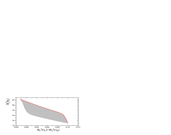
Figure 2: The $1\sigma$ area in the $B_{2}^{g}-B_{2}^{q}$ plane estimated within the RC method by comparing the CLEO data and the theoretical predictions for the resummed and scaled transition FFs $\eta\gamma$, $\eta^{\prime}\gamma$.

The results shown in Figs. 1 – 9—with the exception of Fig. 7—are obtained within the ordinary octet-singlet mixing scheme. In Fig. 1 the predictions for the $\eta\gamma$ and $\eta^{\prime}\gamma$ FFs are presented for $B_{2}^{q}(\eta_{1})=B_{2}^{q}(\eta_{8})=0.02$ and various values of $B_{2}^{g}(\eta_{1})$. One appreciates that without the gluon contribution ($B_{2}^{g}(\eta_{1})=0$) both FFs are slightly below the data points, especially $Q^{2}F_{\eta^{\prime}\gamma}(Q^{2})$. But their deviations are not dramatic and to improve the agreement with the data, one has to include the contribution coming from the gluon component of the $\eta_{1}\gamma$ transition FF. The corresponding results are shown in Fig. 1 by broken lines. These numerical calculations demonstrate that the gluonic contribution is important

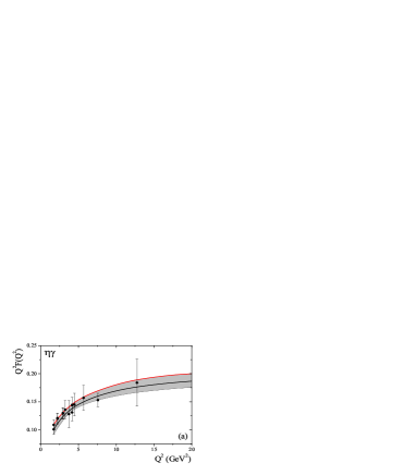
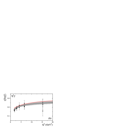
Figure 3: The $\eta\gamma$ (left) and $\eta^{\prime}\gamma$ (right) scaled transition form factors as functions of $Q^{2}$. The central solid curves are found using the values $B_{2}^{q}(\eta_{1})=B_{2}^{q}(\eta_{8})=0.05$ and $B_{2}^{g}(\eta_{1})=17$. The shaded areas demonstrate $1\sigma$ regions for the transition FFs.

Figure 4: The dependence of the $\eta\gamma$ (left panel) and $\eta^{\prime}\gamma$ (right panel) scaled transition form factors on the values of the decay constants $f_{1}$ and $f_{8}$. The octet-singlet mixing angle is $\theta_{p}=-15.4^{\circ}$. The solid curves in both panels are calculated using $f_{1}/f_{\pi}=1.17$, $f_{8}/f_{\pi}=1.26$. The long-dashed curves correspond to $f_{1}/f_{\pi}=1.17$, $f_{8}/f_{\pi}=1.24$ and the short-dashed one in the left panel are found by employing the values $f_{1}/f_{\pi}=1.17$, $f_{8}/f_{\pi}=1.30$. The dash-dotted curves in both panels describe FFs obtained with $f_{1}/f_{\pi}=1.20$ and $f_{8}/f_{\pi}=1.28$.

at relatively low values of the momentum-transfer $Q^{2}$. From Fig. 1 it is clear that the gluonic contribution, arising from the $\eta_{1}$ DA with $B_{2}^{g}(\eta_{1})>0$, enhances the transition FFs $Q^{2}F_{\eta\gamma}(Q^{2})$ and $Q^{2}F_{\eta^{\prime}\gamma}(Q^{2})$ in the region $1.5\;{\rm GeV}^{2}\leq Q^{2}\leq 12\;{\rm GeV}^{2}$ while reducing their magnitude at $Q^{2}>12\;{\rm GeV}^{2}$. This effect is sizeable for the $\eta^{\prime}\gamma$ transition FF relative to its counterpart for $\eta\gamma$, in particular, for larger values of $B_{2}^{g}(\eta_{1})$ and for smaller values of $B_{2}^{g}(\eta_{1})$. The impact of the gluonic contribution on the $\eta\gamma,\;\eta^{\prime}\gamma$ transition FFs is quite understandable, recalling that the physical $\eta$ and $\eta^{\prime}$ states consist predominantly of the flavor $SU_{f}(3)$ octet $\eta_{8}$ and singlet $\eta_{1}$ states, respectively, with the $\eta_{1}\gamma$ transition FF comprising also a gluonic part. Therefore, the $\eta^{\prime}\gamma$ transition FF should be and is more sensitive to the gluonic part.

These features of the $\eta\gamma$ and $\eta^{\prime}\gamma$ transition FFs determine the $1\sigma$ region for the allowed values of the Gegenbauer coefficients $B_{2}^{q}(\eta_{1})=B_{2}^{q}(\eta_{8})$ and $B_{2}^{g}(\eta_{1})$, plotted in Fig. 2. In other words, the $\eta\gamma$ and $\eta^{\prime}\gamma$ transition FFs, computed in the context of the RC method by employing the model DAs with input parameters belonging to the shaded region in Fig. 2, describe the CLEO data with a $1\sigma$ accuracy.

In Fig. 3 we plot the $1\sigma$ areas for the $\eta\gamma$ and $\eta^{\prime}\gamma$ transition FFs. If we were to consider the $\eta\gamma$ and $\eta^{\prime}\gamma$ transitions separately, these areas would be larger than those shown in Fig. 3. For the $\eta\gamma$ transition, the upper bound of the $1\sigma$ region can be extended towards larger values of $Q^{2}F_{\eta\gamma}(Q^{2})$. For the $\eta^{\prime}\gamma$ transition, the lower bound of the corresponding $1\sigma$ region can be shifted towards lower values of $Q^{2}F_{\eta^{\prime}\gamma}(Q^{2})$. But their joint treatment leads to the picture drawn in Fig. 3.

Figure 5: The dependence of the $\eta\gamma$ (left panel) and $\eta^{\prime}\gamma$ (right panel) scaled transition form factors on the octet-singlet mixing angle $\theta_{p}$. The solid curves describe the “default” choice $\theta=-15.4^{\circ}$. The dashed curves correspond to $\theta=-16.4^{\circ}$ and the dash-dotted ones to $\theta=-14.4^{\circ}$.

A major problem in extracting the values of theoretical parameters from the experimental data is their stability against uncertainties inherent in the theoretical expressions. In the case under consideration, expressions (4), (39), and (40) for the $\eta\gamma$ and $\eta^{\prime}\gamma$ transition FFs depend on the factorization scale, on the QCD scale parameter $\Lambda$, the decay constants $f_{1},\;f_{8}$, and the octet-singlet mixing angle $\theta_{p}$. As we have explained in Sec. III, the renormalization scale $\mu_{\rm R}^{2}$ ($\overline{\mu}_{\rm R}^{2}$) in the context of the RC method is determined by the hard-scattering dynamics of the underlying partonic subprocess and is not a free parameter. Our analytical expressions for the transition FFs, calculated by keeping $\mu_{\rm F}^{2}\neq Q^{2}$, allow us to analyze the dependence of the extracted parameters $B_{2}^{q}(\eta_{1}),\;B_{2}^{q}(\eta_{8})$, and $B_{2}^{g}(\eta_{1})$ on the factorization scale $\mu_{\rm F}^{2}$. We have performed the computation of the $\eta\gamma$ and $\eta^{\prime}\gamma$ transition FFs using the values $\mu_{\rm F}^{2}=Q^{2}/2$ and $\mu_{\rm F}^{2}=2Q^{2}$ and found that our prediction for the $1\sigma$ area (Fig. 2) is absolutely stable against these variations. This means that the FFs determined by the input parameters from the $1\sigma$ area in Fig. 2, by varying the factorization scale, remain within the corresponding $1\sigma$ regions shown in Fig. 3. Stated differently, the variation of $\mu_{\rm F}^{2}$ in the limits $\mu_{\rm F}^{2}\in[1/2,\ 2]Q^{2}$ does not change (shift, rotate) the $1\sigma$ area in Fig. 2. On the contrary, the variation of the QCD scale parameter $\Lambda$ modifies the $1\sigma$ region in Fig. 2. The entailed modifications shift the region along both axes, retaining, however, its form stable. Thus, computations performed with $\Lambda_{4}=0.26\ {\rm GeV}$ result in the following shifts: along the $B_{2}^{q}(\eta_{1})=B_{2}^{q}(\eta_{8})$ axis: $\sim 0.005$, along the $B_{2}^{g}(\eta_{1})$ axis: $\sim 1$. Hence, the modification of the $1\sigma$ area is $\sim 9\%$ in the first and $\sim 6\%$ in the second direction, respectively, the percentages being given relative to the central values (see, Eq. (63) below).

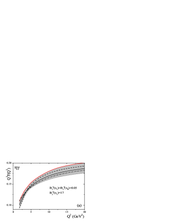
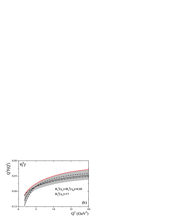
Figure 6: The $\eta\gamma$ (left panel) and $\eta^{\prime}\gamma$ (right panel) scaled transition form factors as functions of $Q^{2}$. All predictions have been obtained within the ordinary mixing scheme and using the initial input parameters (11) and (56). The broken lines denote the FFs with the uncertainties included via Eq. (48), and using the following values of $\{N_{q}\},\;q=1,2,3,4$ : 0.9 (dashed lines); -0.6 (dash-dotted lines).

The response of the central curves (Fig. 3) on variations of the decay constants $f_{1},\;f_{8}$, and such due to the octet-singlet mixing angle $\theta_{p}$ within corresponding phenomenologically allowed ranges FKS98 , is demonstrated in Figs. 4 and 5. It is remarkable that under these variations the central curves remain entirely within the associated $1\sigma$ areas for the $\eta\gamma$ and $\eta^{\prime}\gamma$ transition FFs. It turns out that the $\eta\gamma$ transition FF is more sensitive to the value of the decay constant $f_{8}$ than the $\eta^{\prime}\gamma$ one. The results for the $\eta^{\prime}\gamma$ transition FF obtained by varying the constant $f_{8}\in[1.24,\;1.30]f_{\pi}$ at fixed $f_{1}=1.17f_{\pi}$ practically coincide with each other. On the contrary, the $\eta^{\prime}\gamma$ transition FF demonstrates a rather strong dependence on the decay constant $f_{1}$, whereas the $\eta\gamma$ one is stable under such variations (cf. the short-dashed and dash-dotted curves, respectively, in Fig. 4(a)). Our computations with $\theta_{p}=-15.4^{\circ}\pm 1^{\circ}$ confirm the conclusion drawn in Ref. Aga01 that the FF for the $\eta\gamma$ transition is more sensitive to $\theta_{p}$ than the one for the $\eta^{\prime}\gamma$ transition. Summing up, we can state that the modification of the central curves in Figs. 4 and 5, due to the variations of the decay constants and the mixing angle discussed above, does not exceed the level of $\pm 3\%$ of their values.

In Sec. III we have emphasized that the ambiguities produced by the principal value prescription, inherent in the RC method, affect the predictions for the transition FFs in accordance with Eq. (48). The ambiguity $[Q^{2}F_{\rm M\gamma}^{1(8)}(Q^{2})]^{\rm amb}$ depends on the $\eta_{1}$ and $\eta_{8}$ DAs and also on the constant $\{N_{q}\}$. In reality, however, for given DAs of the $\eta_{1}$ and $\eta_{8}$ states, the available experimental information allows one to extract constraints on $\{N_{q}\}$. To effect the influence of such contributions, we show exemplarily in Fig. 6 predictions for the FFs with and without such ambiguities, utilizing the expansion coefficients $B_{2}^{q}(\eta_{1})=B_{2}^{q}(\eta_{8})=0.05,\,B_{2}^{g}(\eta_{1})=17$. We find that in order that the FFs remain within the corresponding $1\sigma$ regions, the upper and lower bounds, respectively, for the constants $\{N_{q}\}$ are provided by the values $\{N_{q}=0.9\}$ and $\{N_{q}=-0.6\}$. Hence, the $\eta\gamma$ transition FFs with the ambiguities included, corresponding to $\{N_{q}=-0.6\}$ ($\{N_{q}=0.9\}$) at $Q^{2}<4~{}{\rm GeV}^{2}$, are larger (smaller) than the FFs without such corrections and are, in addition, smaller (larger) for $Q^{2}>4~{}{\rm GeV}^{2}$. For the $\eta^{\prime}\gamma$ transition FF we observe, qualitatively, the same behavior, but with $Q^{2}\simeq 5~{}{\rm GeV}^{2}$ as the transition momentum scale from the small to the large (and vice versa) regions. In any case, the uncertainties do not exceed the level of $\pm 11\%$ of the corresponding FFs in the region $Q^{2}\sim(1.73-2)\,\,{\rm GeV}^{2}$ and reach a mere $\mp 3\%$ level in the region $Q^{2}\sim(16-20)\,\,{\rm GeV}^{2}$.

Figure 7: The $\eta\gamma$ (a) and $\eta^{\prime}\gamma$ (b) electromagnetic transition FFs vs. $Q^{2}$. The solid lines correspond to the ordinary octet-singlet mixing scheme with parameters $B_{2}^{q}(\eta_{1})=B_{2}^{q}(\eta_{8})=0.02$ and $B_{2}^{g}(\eta_{1})=18$. The broken lines are obtained within the two-mixing angle scheme. The dashed lines describe the situation with the same parameters as the solid curves. The parameters for the dash-dotted curves are $B_{2}^{q}(\eta_{1})=B_{2}^{q}(\eta_{8})=0.15,\,B_{2}^{g}(\eta_{1})=18$.

Below, we present sample estimates for the eigenfunctions expansion coefficients of the $\eta_{1}$ and $\eta_{8}$ DAs in the context of the ordinary mixing scheme:

$$B_{2}^{q}(\eta_{1})=0\,,\;B_{2}^{q}(\eta_{8})=0\,,\;B_{2}^{g}(\eta_{1})\in[17,\,21.5]\,,$$ (58)

$$B_{2}^{q}(\eta_{1})=0.02\,,\;B_{2}^{q}(\eta_{8})=0.02\,,\;B_{2}^{g}(\eta_{1})\in[16,\,20.5]\,,$$ (59)

$$B_{2}^{q}(\eta_{1})=0.05\,,\;B_{2}^{q}(\eta_{8})=0.05\,,\;B_{2}^{g}(\eta_{1})\in[15,\,19]\,,$$ (60)

and

$$B_{2}^{q}(\eta_{1})=0.1\,,\;B_{2}^{q}(\eta_{8})=0.1\,,\;B_{2}^{g}(\eta_{1})\in[13.5,\,17]\,.$$ (61)

The constraints (58)–(61) on the input parameter $B_{2}^{g}(\eta_{1})$ are extracted for fixed coefficients $B_{2}^{q}(\eta_{1})$ and $B_{2}^{q}(\eta_{8})$, and represent the $1\sigma$ range for the values of $B_{2}^{g}(\eta_{1})$ compatible with the CLEO data. Restrictions on the parameters $B_{2}^{q}(\eta_{1})$ and $B_{2}^{q}(\eta_{8})$ at fixed value of $B_{2}^{g}(\eta_{1})$ can also be derived. For example, for $B_{2}^{g}(\eta_{1})=16$, we get

$$B_{2}^{g}(\eta_{1})=16,\;B_{2}^{q}(\eta_{1})=B_{2}^{q}(\eta_{8})\in[0.02,\,0.11]\,.$$ (62)

Summarizing this point, the estimates for the Gegenbauer coefficients $B_{2}^{q}(\eta_{1}),\,B_{2}^{q}(\eta_{8})$ and $B_{2}^{g}(\eta_{8})$ in the DAs for the $\eta_{1},\;\eta_{8}$ states are

$$B_{2}^{q}(\eta_{1})=B_{2}^{q}(\eta_{8})=0.055\pm 0.065,\;\;B_{2}^{g}(\eta_{1})=18\mp 4.5.$$ (63)

Here some comments concerning the usual octet-singlet mixing scheme (10) and the parameter set (11) are in order. These parameters were extracted from the analysis of the CLEO data using the two-mixing-angles scheme, but staying within the context of the hard-scattering approach of perturbative QCD. Our computations demonstrate that adopting the RC method, the parameters given by (11) satisfactorily describe these data, provided one uses the usual octet-singlet mixing scheme. Therefore, one can consider the parameters (11) as a prediction of the RC method and the one-angle mixing scheme. This prediction differs from those obtained already within the one-angle mixing scheme, but employing the traditional theoretical methods (see, for example, Ref. ONS )

However, our calculations do not exclude the usage of the two-mixing-angle scheme in conjunction with the RC method. But in such a case, a considerably larger contribution of the nonasymptotic terms to the DAs of the $\eta_{1}$ and $\eta_{8}$ states would be required. Carrying out such a computation via (12), (13), we obtained the results shown in Fig. 7. Inspection of Fig. 7(a) reveals that the $\eta\gamma$ transition FF found within this scheme lies significantly lower than the data. Therefore, to improve the results, a relatively large contribution of the first Gegenbauer polynomial to the DAs of the $\eta_{1}$ and $\eta_{8}$ states seems necessary. In Fig. 7 we display the FFs obtained using the parameters $B_{2}^{q}(\eta_{1})=0.15,\;B_{2}^{q}(\eta_{8})=0.15$ and $B_{2}^{g}(\eta_{1})=18$. We consider the values $B_{2}^{q}(\eta_{1})=B_{2}^{q}(\eta_{8})=0.15$ as determining the lower bound for the admissible set of DAs in the context of the two-mixing-angles parametrization scheme. Hence, in the two-mixing-angles scheme, we obtain

$$B_{2}^{q}(\eta_{1})=B_{2}^{q}(\eta_{8})=0.15,\;B_{2}^{g}(\eta_{1})\in[16,\,20]\,.$$ (64)

Figure 8: The $\eta\gamma$ scaled transition FF vs. $Q^{2}$. In the computations the ordinary octet-singlet mixing scheme is used. The upper (lower) bundle of curves is found within the standard HSA (RC method). The correspondence between the curves and the input parameters is as follows: for the solid curves $B_{2}^{q}(\eta_{1})=B_{2}^{q}(\eta_{8})=0,\,B_{2}^{g}(\eta_{1})=0$; for the dashed lines $B_{2}^{q}(\eta_{1})=B_{2}^{q}(\eta_{8})=-0.05,\,B_{2}^{g}(\eta_{1})=0$; for the dash-dotted ones $B_{2}^{q}(\eta_{1})=B_{2}^{q}(\eta_{8})=0.1,\,B_{2}^{g}(\eta_{1})=0$, and for the short-dashed curves $B_{2}^{q}(\eta_{1})=B_{2}^{q}(\eta_{8})=0.1,\,B_{2}^{g}(\eta_{1})=15$.

The $\eta$ and $\eta^{\prime}$ DAs were extracted from the CLEO data on the $\eta\gamma$ and $\eta^{\prime}\gamma$ transition FFs KP02 having also recourse to the $\eta^{\prime}$-meson energy spectrum in the decay $\Upsilon(1S)\to\eta^{\prime}X$ AP03 . In both these papers the standard HSA was employed. In Ref. KP02 , estimates for the parameters $B_{2}^{1}(\mu_{0}^{2}),\;B_{2}^{g}(\mu_{0}^{2})$, and $B_{2}^{8}(\mu_{0}^{2})$ were made within the two-mixing-angles scheme (12), reading

$$B_{2}^{1}(1\,\,\,{\rm GeV}^{2})=-0.08\pm 0.04\,,\;B_{2}^{g}(1\,\,{\rm GeV}^{2})=9\pm 12\,,\;B_{2}^{8}(1\,\,{\rm GeV}^{2})=-0.04\pm 0.04\,.$$ (65)

These coefficients are related to ours through the expressions

$$B_{2}^{1}(\mu_{0}^{2})=\frac{A(\mu_{0}^{2})}{6}\,,\;B_{2}^{g}(\mu_{0}^{2})=\frac{B(\mu_{0}^{2})}{5}\,,\;B_{2}^{8}(\mu_{0}^{2})=\frac{C(\mu_{0}^{2})}{6}\,.$$ (66)

Using our approach and the one-angle mixing scheme, the values of these parameters were determined to be

$$B_{2}^{1}(1\,\,{\rm GeV}^{2})=-0.214\pm 0.025\,,\;B_{2}^{g}(1\,\,{\rm GeV}^{2})=19.25\pm 2.25\,,\;B_{2}^{8}(1\,\,{\rm GeV}^{2})=0\,,$$

$$B_{2}^{1}(1\,\,{\rm GeV}^{2})=-0.183\pm 0.025\,,\;B_{2}^{g}(1\,\,{\rm GeV}^{2})=18.57\pm 2.25\,,\;B_{2}^{8}(1\,\,{\rm GeV}^{2})=0.02\,,$$

$$B_{2}^{1}(1\,\,{\rm GeV}^{2})=-0.139\pm 0.022\,,\;B_{2}^{g}(1\,\,{\rm GeV}^{2})=17.8\pm 2\,,\;B_{2}^{8}(1\,\,{\rm GeV}^{2})=0.05\,,$$ (67)

$$B_{2}^{1}(1\,\,{\rm GeV}^{2})=-0.07\pm 0.02\,,\;B_{2}^{g}(1\,\,{\rm GeV}^{2})=16.85\pm 1.75\,,\;B_{2}^{8}(1\,\,{\rm GeV}^{2})=0.1\,,$$

and

$$B_{2}^{1}(1\,\,{\rm GeV}^{2})=-0.1128\pm 0.045\,,\;B_{2}^{g}(1\,\,{\rm GeV}^{2})=16.208\pm 0.144\,,\;B_{2}^{8}(1\,\,{\rm GeV}^{2})=0.65\pm 0.045\,.$$ (68)

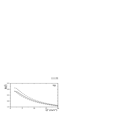
Figure 9: The ratio $R(Q^{2})$ for the $\eta\gamma$ FF. The solid line corresponds to the input parameters $B_{2}^{q}(\eta_{1})=B_{2}^{q}(\eta_{8})=B_{2}^{g}(\eta_{1})=0$. The dash-dotted curve describes the same ratio, but for $B_{2}^{q}(\eta_{1})=B_{2}^{q}(\eta_{8})=0,\,B_{2}^{g}(\eta_{1})=14$, while the dashed one corresponds to $B_{2}^{q}(\eta_{1})=B_{2}^{q}(\eta_{8})=0.05,\,B_{2}^{g}(\eta_{1})=10$.

In the case of the two-mixing-angles scheme, we find

$$B_{2}^{1}(1\,\,{\rm GeV}^{2})=-0.050\pm 0.022\,,\;B_{2}^{g}(1\,\,{\rm GeV}^{2})=20.4\pm 2\,,\;B_{2}^{8}(1\,\,{\rm GeV}^{2})=0.15\,.$$ (69)

One observes that within the two-mixing-angles scheme, the parameters $B_{2}^{1},\,B_{2}^{8}$ obey the constraints $B_{2}^{1}(1\,{\rm GeV}^{2})<0$ and $B_{2}^{8}(1\,{\rm GeV}^{2})>0$ (cf. Eq. (65)).

On the other hand, the constraints for the parameters $B_{2}^{q}(\mu_{0}^{2})$ and $B_{2}^{g}(\mu_{0}^{2})$, extracted in Ref. AP03 at the normalization point $\mu_{0}^{2}=2\,\,{\rm GeV}^{2}$, read

$$B_{2}^{q}(2\;{\rm GeV}^{2})=0.010\pm 0.068,\quad B_{2}^{g}(2\;{\rm GeV}^{2})=5.6\pm 3.4\,.$$ (70)

Comparing now Eq. (70) with the values given in Eq. (64), and taking into account that in Ref. AP03 different values for the scheme parameters defined by Eq. (56) were used, we come to the conclusion that in the context of the RC method and the two-mixing-angles scheme, the region $B_{2}^{q}(2\ {\rm GeV}^{2})<0$ should be excluded as contradicting the CLEO data.

The apparent discrepancy between the results of the present work and those of Ref. KP02 , as regards the extracted values of the coefficients $B_{2}^{1}(1\;{\rm GeV}^{2})$ and $B_{2}^{8}(1\;{\rm GeV}^{2})$, is related to the fact that the employed theoretical schemes are intrinsically different. Indeed, the transition FFs computed in the standard HSA overshoot the CLEO data—especially in the low-momentum transfer regime. In Fig. 8 the $\eta\gamma$ transition FF obtained in the standard HSA and the ordinary octet-singlet mixing scheme is depicted. One appreciates that the deviation from the data is considerable. The DAs corresponding to the parameters $B_{2}^{q}(\eta_{1}),\;B_{2}^{q}(\eta_{8})>0$ even increase this disagreement, whereas by adding the gluon component with $B_{2}^{g}(\eta_{1})>0$ one can reduce it. Therefore to decrease the magnitude of the FFs, and achieve this way a better agreement with the data, the standard HSA would call for the two-mixing-angles scheme and for DAs mainly with $B_{2}^{q}(\eta_{1}),\,B_{2}^{q}(\eta_{8})<0$. The inclusion of power corrections changes this situation radically. In fact, at low-momentum transfer these corrections enhance the absolute value of the NLO correction to the FFs by more than a factor of $2.5-3$ and, because the contribution of the NLO term to the FFs is negative, power corrections reduce the leading-order prediction for the FFs considerably, while at the highest $Q^{2}$ values measured by the CLEO collaboration this influence becomes more moderate. As a result, the $\eta\gamma$ and $\eta^{\prime}\gamma$ transition FFs computed using the input parameters from the $1\sigma$ area in Fig. 2 within the RC method in conjunction with the one-angle mixing scheme are in agreement with the CLEO data. In order to quantify these statements, we show in Fig. 9 the numerical results for the ratio

$$R_{\rm M\gamma}(Q^{2})=\frac{[Q^{2}F_{\rm M\gamma}(Q^{2})]_{\rm NLO}^{\rm res}}{[Q^{2}F_{\rm M\gamma}(Q^{2})]_{\rm NLO}^{\rm HSA}}$$ (71)

for some selected values of the expansion coefficients.

V Concluding remarks

In this work we have performed a computation of the $\eta\gamma$ and $\eta^{\prime}\gamma$ transition FFs within the RC method. The latter has enabled us to estimate a class of power corrections to the FFs related to nonperturbative effects arising from the dependence of the strong coupling on the longitudinal momentum fractions of the partons inside the $\eta$ and $\eta^{\prime}$ mesons after the identification of the renormalization scale with a physical momentum depending on these fractions. This has been achieved by regularizing the infrared singularities ensuing from the end points $x=0,1$ by means of the principal value prescription within the IR renormalon approach. The effect of power-suppressed ambiguities to the considered form factors was addressed and their influence was found to be less important, though not negligible, with contributions varying in the range between $3\%$ at high to $11\%$ at low $Q^{2}$ values.

Contributions to the FFs from the valence quark as well as the two-gluon Fock-state of the $\eta$ and $\eta^{\prime}$ meson DAs have been taken into account. We have obtained the Borel resummed expressions $[Q^{2}F_{\rm M\gamma}(Q^{2})]^{\rm res}$ for the FFs and proved that in the asymptotic limit $Q^{2}\to\infty$ they lead to the standard HSA predictions.

We have demonstrated that the effect of the calculated power corrections on the $\eta\gamma$ and $\eta^{\prime}\gamma$ transition FFs is considerable. Indeed, at moderate values of the momentum-transfer $Q^{2}\leq 5\;{\rm GeV}^{2}$ they turn out to enhance the absolute value of the $O(\alpha_{{\rm s}})$ correction to the FFs more than $2.5-3$ times. The ratio $R_{\rm M\gamma}(Q^{2})$ of the corresponding contributions depends on the specific $M\gamma$ transition under consideration and on the input parameters (Gegenbauer coefficients) of the $\eta$ and $\eta^{\prime}$ meson DAs. These features of the power corrections have important consequences: the enhanced (negative) NLO correction significantly reduces the leading-order contribution to the FFs, so that the input parameters of the $\eta$ and $\eta^{\prime}$ meson DAs, which correctly describe the CLEO data within the RC method, must obey the constraints presented in Fig. 2 by the shaded $1\sigma$ area to fulfill Eq. (63). It is worth emphasizing that our predictions for the $\eta$ and $\eta^{\prime}$ meson DAs disagree with those extracted from the CLEO data in the context of the standard HSA.

The DAs of the $\eta$ and $\eta^{\prime}$ mesons obtained in this work can be useful in the investigation of other exclusive processes that involve $\eta$ and $\eta^{\prime}$ mesons, especially at lower momentum-transfer values, where the standard HSA is most unreliable.

References

(1) S. S. Agaev,
Phys. Rev. D 64, 014007 (2001).
(2) S. S. Agaev and A. I. Mukhtarov,
Int. J. Mod. Phys. A 16, 3179 (2001).
(3) J. Cao, F.-G. Cao, T. Huang, and B.-Q. Ma,
Phys. Rev. D 58, 113006 (1998)
[hep-ph/9807508].
(4) R. Jakob, P. Kroll, and M. Raulfs,
J. Phys. G 22, 45 (1996)
[hep-ph/9410304];
P. Kroll and M. Raulfs,
Phys. Lett. B 387, 848 (1996)
[hep-ph/9605264];
Th. Feldmann and P. Kroll,
Eur. Phys. J. C 5, 327 (1998)
[hep-ph/9711231];
M. Diehl, P. Kroll, and C. Vogt,
Eur. Phys. J. C 22, 439 (2001)
[hep-ph/0108220].
(5) N. G. Stefanis, W. Schroers, and H. C. Kim,
Phys. Lett. B 449, 299 (1999)
[hep-ph/9807298];
Eur. Phys. J. C 18, 137 (2000)
[hep-ph/0005218].
(6) P. Kroll and K. Passek-Kumerički,
Phys. Rev. D 67, 054017 (2003)
[hep-ph/0210045].
(7) A. Khodjamirian,
Eur. Phys. J. C 6, 477 (1999)
[hep-ph/9712451].
(8) A. Schmedding and O. Yakovlev,
Phys. Rev. D 62, 116002 (2000)
[hep-ph/9905392].
(9) A. P. Bakulev, S. V. Mikhailov, and N. G. Stefanis,
Phys. Rev. D 67, 074012 (2003)
[hep-ph/0212250];
Phys. Lett. B 578, 91 (2004)
[hep-ph/0303039];
[hep-ph/0312141].
(10) Y. V. Mamedova,
Int. J. Mod. Phys. A 18, 1023 (2003).
(11) CLEO Collaboration,
J. Gronberg et al.,
Phys. Rev. D 57, 33 (1998)
[hep-ex/9707031].
(12) M. K. Chase,
Nucl. Phys. B174, 109 (1980);
V. N. Baier and G. Grozin,
Nucl. Phys. B192, 476 (1981);
M. V. Terentyev,
Sov. J. Nucl. Phys. 33, 911 (1981)
[Yad. Fiz. 33, 1692 (1981)].
(13) S. S. Agaev and N. G. Stefanis,
Eur. Phys. J. C 32, 507 (2004)
[hep-ph/0212318].
(14) G. P. Lepage and S. J. Brodsky,
Phys. Rev. D 22, 2157 (1980);
A. V. Efremov and A. V. Radyushkin,
Phys. Lett. B 94, 245 (1980);
Theor. Math. Phys. 42, 97 (1980)
[Teor. Mat. Fiz. 42, 147 (1980)];
A. Duncan and A. H. Mueller,
Phys. Rev. D 21, 1636 (1980).
(15) S. S. Agaev,
Phys. Lett. B 360, 117 (1995)
[Erratum-ibid, B 369, 379 (1996)];
[hep-ph/9611215].
(16) S. S. Agaev,
Mod. Phys. Lett. A 10, 2009 (1995);
ibid. A 11, 957 (1996);
ibid. A 13, 2637 (1998)
[hep-ph/9805278].
(17) D. V. Shirkov and I. L. Solovtsov,
Phys. Rev. Lett. 79, 1209 (1997)
[hep-ph/9704333].
(18) A. I. Karanikas and N. G. Stefanis,
Phys. Lett. B 504, 225 (2001)
[hep-ph/0101031].
(19) N. G. Stefanis,
in 8th Adriatic Meeting and Central
European Symposia on Particle Physics in the New Millennium,
Dubrovnik, Croatia, 4-14 September 2001, published in Lect. Notes Phys. 616, 153 (2003)
[hep-ph/0203103].
(20) F. del Aguila and M. K. Chase,
Nucl. Phys. B193, 517 (1981);
E. Braaten,
Phys. Rev. D 28, 524 (1983);
E. P. Kadantseva, S. V. Mikhailov, and A. V. Radyushkin,
Sov. J. Nucl. Phys. 44, 326 (1986)
[Yad. Fiz. 44, 507 (1986)].
(21) B. Melić, B. Nižić, and K. Passek,
Phys. Rev. D 65, 053020 (2002)
[hep-ph/0107295].
(22) Th. Feldmann, P. Kroll, and B. Stech,
Phys. Rev. D 58, 114006 (1998)
[hep-ph/9802409].
(23) A. P. Bakulev, S. V. Mikhailov and N. G. Stefanis,
Phys. Lett. B 508, 279 (2001)
[hep-ph/0103119];
in Proceedings of the 36th Rencontres de Moriond
on QCD and Hadronic Interactions, 17-24 Mar 2001,
Les Arcs, France, 133-136
[hep-ph/0104290];
hep-ph/0310267.
(24) A. P. Bakulev and S. V. Mikhailov
Phys. Rev. D 65, 114511 (2002)
[hep-ph/0203046].
(25) V. Y. Petrov et al.,
Phys. Rev. D 59, 114018 (1999)
[hep-ph/9807229]
M. Praszalowicz and A. Rostworowski,
Phys. Rev. D 64, 074003 (2001)
[hep-ph/0105188];
I. V. Anikin, A. E. Dorokhov, and L. Tomio,
Phys. Part. Nucl. 31, 509 (2000);
A. E. Dorokhov,
JETP Lett. 77, 63 (2003).
(26) S. J. Brodsky, G. P. Lepage, and P. B. Mackenzie,
Phys. Rev. D 28, 228 (1983).
(27) M. Beneke,
Phys. Rep. 317, 1 (1999)
[hep-ph/9807443].
(28) P. Gosdzinsky and N. Kivel,
Nucl. Phys. B521, 274 (1998)
[hep-ph/9707367].
(29) S. V. Mikhailov,
Phys. Lett. B 431, 387 (1998)
[hep-ph/9804263].
(30) E. Braaten and Y.-Q. Chen,
Phys. Rev. D 57, 4236 (1998),
[Erratum-ibid. D 59, 079901 (1999)]
[hep-ph/9710357].
(31) R. Akhoury, A. Sinkovics, and M. G. Sotiropoulos,
Phys. Rev. D 58, 013011 (1998)
[hep-ph/9709497].
(32) H. Contopanagos, G. Sterman,
Nucl. Phys. B 419,
77 (1994) [hep-ph/9310313].
(33) G. ’t Hooft, in Whys of Subnuclear Physics, Proceeding
of the International School, Erice, 1977, edited by
A. Zichichi (Prenum, New York 1978);
A. I. Zakharov, Nucl. Phys. B 385, 452 (1992).
(34) B. R. Webber,
J. High Energy Physics 10, 012 (1998)
[hep-ph/9805484].
(35) S. S. Agaev,
Nucl. Phys. B (Proc. Suppl.) 74, 155 (1999)
[hep-ph/9807444].
(36) A. Ali and A. Ya. Parkhomenko,
Eur. Phys. J. C 30, 183 (2003)
[hep-ph/0304278].
(37) E. P. Venugopal and Barry R. Holstein,
Phys. Rev. D 57, 4397 (1998)
[hep-ph/9710382].