Kinks in the Hartree approximation

Abstract

The topological defects of $\lambda\phi^{4}$ theory, the kink and antikink, are studied in the Hartree approximation. This allows us to discuss quantum effects on defects in both stationary and dynamical systems. The kink mass is calculated for a number of parameters, and compared to classical, one loop and Monte Carlo results known from the literature. We discuss the thermalization of the system after a kink-antikink collision. A classical result, the existence of a critical speed, is rederived and shown for the first time in the quantum theory. We also use kink-antikink collisions as a very simple toy model for heavy ion collisions and discuss the differences and similarities, for example in the pressure. Finally, using the Hartree Ensemble Approximation allows us to study kink-antikink nucleation starting from a thermal (Bose-Einstein) distribution. On a qualitative level, our results show only few dissimilarities with the classical results, but on a quantitative level there are some important differences.

I Introduction

In recent years the increasing numerical power of computers has made it possible to follow quantum fields in real time, studying phenomena such as thermalization, phase transitions and the formation of topological defects. Until recently this was mainly done using the classical approximation, which can be justified when occupation numbers are large. However, this is never the case for all momentum modes, and for systems far from equilibrium, this approximation may also break down. The Hartree and large-$n$ approximations do capture quantum effects but, until recently, the available numerical power did not allow for the simulation of inhomogeneous systems, thereby excluding the study of many physically interesting phenomena such as topological defects. It also has problems with describing thermalization, due to the lack of direct scattering. Recently, approximations based on an expansion of the $2PI$ effective action (see Ref. Aarts et al. (2002) and references therein) and also on a truncation of Schwinger-Dyson equations (see Ref. Cooper et al. (2003) and references therein), which do include direct scattering have been shown to lead to a quantum thermal equilibrium. Unfortunately, these methods are still numerically expensive and are not yet able to describe inhomogeneous systems. In two papers Sallé et al. (2001, 2002) we introduced the Hartree ensemble approximation, which tries to combine the good features of both the classical approximation, which is able to thermalize (classically), and the Hartree approximation, being a quantum approximation and thus free from the Rayleigh-Jeans divergencies. In the Hartree ensemble approximation, the initial density matrix is expanded on a (overcomplete) basis of Gaussian density matrices. Expectation values can then be written as a weighted average of Gaussian expectation values. The equations of motion are derived using the Hartree approximation in each of the “realizations.” The partial “mean fields” of these different “realizations,” i.e., the expectation values of the field in the different Gaussian initial states, are typically inhomogeneous and the interaction of the quantum modes with the Fourier modes of these “mean fields” leads to approximately thermal distributions. However, since these “mean fields” are typically inhomogeneous, topological defects can and will be present if the symmetries of the theory allow for them. These will be the topic of this paper, we will look at the $\phi^{4}$ theory in 1+1 dimensions and its defects, kinks, and make a comparison between the classical theory and the Hartree approximation.

The rest of the paper in organised as follows. We will, in the remainder of this introduction, briefly review the equations of motion and our definition of instantaneous particle number, used in studying the distribution function. In Sec. II we will derive the classical kink solutions, as this will facilitate comparison with the Hartree approximation. Then, in Sec. III, we will discuss Hartree kink-antikink pairs, initially at rest and compare with the classical approximation. A study of the Hartree kink mass will be made. In Sec. IV kink-antikink collisions will be studied. We will look at the critical speed: below a certain speed the pair annihilates, while above they bounce back. This has been extensively discussed for the classical theory, but not yet for the quantum theory. We will study whether the system thermalizes after the collision and use the collisions as a toy model for heavy ion collisions, looking at the central region and its dependency on coupling and initial speed. As a final topic we will, in Sec. V, look at thermal kink nucleation, starting from a Bose-Einstein thermal ensemble, as in Ref. Sallé et al. (2002). The conclusions are in Sec. VI.

I.1 Equations of motion

In this section we very briefly discuss the Hartree equations of motion for the $\phi^{4}$ theory, as used in the separate “realizations” of the initial ensemble. For more information see Refs. Sallé et al. (2001, 2002); Sallé and Smit (2003).

The Lagrangian density for our 1+1 dimensional system is given by

$$\mathcal{L}=-\frac{1}{2}\partial_{\mu}\phi\partial^{\mu}\phi-\frac{1}{2}\mu^{2}\phi^{2}-\frac{1}{4}\lambda\phi^{4},$$ (1)

giving rise to the Heisenberg (operator) equations of motion

$$-\partial_{\mu}\partial^{\mu}\hat{\phi}+\mu^{2}\hat{\phi}+\lambda\hat{\phi}^{3}=0.$$ (2)

By introducing expectation values of products of field operators one obtains a hierarchy of equations: the equation for the $n$-point function will contain also the $(n+2)$-function. Unless the initial density matrix, which is used in the calculation of the expectation values, is Gaussian, this hierarchy will be infinite. The Hartree approximation truncates it self-consistently by imposing Gaussianity, thus factorizing all $n$-point functions with $n>2$ into $1$- and $2$-point functions. It is convenient to expand the $2$-point function in a set of mode functions, which in the free theory are simply plane waves. This expansion is most easily implemented in the field operator itself

$$\hat{\phi}(x,t)=\phi(x,t)+\sum_{\alpha}f_{\alpha}(x,t)\hat{b}_{\alpha}+h.c.$$ (3)

It is important to note that, due to the Hartree approximation, the creation and annihilation operators $\hat{b}_{\alpha}$ and $\hat{b}^{\dagger}_{\alpha}$ can be chosen time-independent. They also satisfy the usual commutation relations. The complex mode functions $f_{\alpha}(x,t)$ form a complete and orthogonal basis with a Klein-Gordon-type inner product. However, the $\alpha$-label in general does not coincide with the Fourier label in time-dependent systems.

The Heisenberg equations of motion in the Hartree approximation can thus be written as

$$\ddot{\phi} =\Delta\makebox[9.55458pt]{$\phi$}-[\mu^{2}+\hphantom{3}\lambda\phi^{2}+3\lambda C]\phi,$$ (4a)

$$\ddot{f}_{\alpha} =\Delta\makebox[9.55458pt]{$f_{\alpha}$}-[\mu^{2}+3\lambda\phi^{2}+3\lambda C]f_{\alpha},$$ (4b)

with

$$C=\sum_{\alpha}(2n_{\alpha}^{0}+1)|f_{\alpha}|^{2},\qquad n_{\alpha}^{0}=\langle\hat{b}^{\dagger}_{\alpha}\hat{b}_{\alpha}\rangle.$$ (4c)

In $1+1$-dimensions, only the mass needs renormalization, due to the divergence of the mode sum $C(x,t)$. We will do this by absorbing its divergent vacuum part in $\mu^{2}$. In terms of the renormalized $\mu_{\text{ren}}^{2}$ we have obtained a finite theory. In the rest of the paper we will only consider states for which $n_{\alpha}^{0}=0$.

I.2 Observables: Particle number

In order to study thermalization we use the same definition for particle number as before Sallé et al. (2001, 2002); Sallé and Smit (2003), using the $2$-point functions.

$$S(t,x-y) =\overline{\mbox{$\langle\hat{\phi}(t,x)\hat{\phi}(t,y)\rangle$}}-\overline{\mbox{$\langle\hat{\phi}(t,x)\rangle$}}\;\overline{\mbox{$\langle\hat{\phi}(t,y)\rangle$}},$$ (5a)

$$U(t,x-y) =\overline{\mbox{$\langle\hat{\pi}(t,x)\hat{\pi}(t,y)\rangle$}}-\overline{\mbox{$\langle\hat{\pi}(t,x)\rangle$}}\;\overline{\mbox{$\langle\hat{\pi}(t,y)\rangle$}},$$ (5b)

where the overline denotes an average over the center of mass coordinate and optionally a time interval and/or ensemble of initial conditions:

$$\overline{\mbox{$\langle\hat{\phi}(t,y+z)\hat{\phi}(t,y)\rangle$}}=\\ \frac{1}{N}\sum_{\text{ens.}}\frac{1}{L\delta}\int_{t-\delta/2}^{t+\delta/2}dt^{\prime}\int_{0}^{L}dy\mbox{$\langle\hat{\phi}(t^{\prime},y+z)\hat{\phi}(t^{\prime},y)\rangle$},$$ (6)

where $N$ is the number of ensemble members, $L$ the lattice size and $\delta$ a small time interval. In principle the (asymmetric part of the) $\phi\pi$ correlation function could also be used, but as it vanishes in equilibrium, we will refrain from doing that.

We can split the $2$-point functions in the separate contributions from the mean field and the mode functions:

$$S(t,x-y)=S^{c}(t,x-y)+S^{q}(t,x-y),$$ (7)

where

$$S^{c}(t,x-y) =\overline{\phi(t,x)\phi(t,y)}-\overline{\phi(t,x)}\;\overline{\phi(t,y)},$$ (8a)

$$S^{q}(t,x-y) =\overline{C(t,x;t,y)},$$ (8b)

and similarly for $U(t,x-y)$. These expressions only depend on the relative coordinate $x-y$. We take the Fourier transform

$$S_{k}(t)=\frac{1}{L}\int_{0}^{L}dz\;e^{-ikz}\,S(t,z),$$ (9)

with $k=(0,\pm 1,\pm 2,\cdots)(2\pi/L)$. Analogously to their expressions for a free theory we can use them to define instantaneous particle numbers:

$$S_{k}(t) =\left[n_{k}(t)+\frac{1}{2}\right]\frac{1}{\omega_{k}(t)},$$ (10a)

$$U_{k}(t) =\left[n_{k}(t)+\frac{1}{2}\right]\,\omega_{k}(t).$$ (10b)

From these relations we can extract $n_{k}(t)$ and $\omega_{k}(t)$ as a function of time. Compared to other definitions of particle number, this one has the advantage of being manifestly real, thus making them particularly suitable for studying out-of-equilibrium systems.

II Classical kink solutions

When looking for stable solutions to the classical equations of motion of the $\phi^{4}$ theory in an infinite volume, the field has to be in the vacuum at spatial infinity in order to keep the energy finite. In the “broken phase” this still leaves some important freedom. For the trivial solution both ends will be in the same vacuum. However, there is also a nontrivial solution, where the field is in the different vacua in the different spatial infinities and hops over the central barrier somewhere in between. This is the so-called (anti)kink solution. The exact location of the kink does not influence the energy and an infinite set of degenerate solutions exists, but transforming the kink solution into the trivial solution would cost an infinite amount of energy, and hence the topology has rendered it stable. See Ref. Rajaraman (1982) for a standard introduction into the topic.

It is possible to calculate this lowest non-trivial solution using a very elegant and general method, the Bogomol’nyi equation Bogomol’nyi (1976). In the broken phase the classical static Hamiltonian (energy) is given by

$$E =\int dx\,\frac{1}{2}(\phi^{\prime})^{2}+\frac{\lambda}{4}\bigl{(}\phi^{2}-v^{2}\bigr{)}^{2}$$

$$=\int dx\,\biggl{\{}\frac{1}{2}\biggl{(}\phi^{\prime}\pm\sqrt{\frac{\lambda}{2}}\bigl{(}\phi^{2}-v^{2}\bigr{)}\biggr{)}^{2}\mp\phi^{\prime}\sqrt{\frac{\lambda}{2}}\bigl{(}\phi^{2}-v^{2}\bigr{)}\biggr{\}}$$

$$=\int dx\,\frac{1}{2}\biggl{(}\phi^{\prime}\pm\sqrt{\frac{\lambda}{2}}\bigl{(}\phi^{2}-v^{2}\bigr{)}\biggr{)}^{2}$$

$$\hphantom{=}\mp\biggl{[}\sqrt{\frac{\lambda}{2}}\bigl{(}\frac{1}{3}\phi^{3}-v^{2}\phi\bigr{)}\biggr{|}_{\phi(-\infty)}^{\phi(\infty)},$$ (11)

where $\phi^{\prime}=\partial_{x}\phi$. The boundary term is equal to a finite constant and determines the topological sector, trivial or nontrivial. For given boundaries the energy is therefore bounded from below by the first term which is larger than, or equal to zero, the so-called Bogomol’nyi bound. The lowest energy state can be found by solving the simple first order differential equation

$$\phi^{\prime}=\mp\sqrt{\frac{\lambda}{2}}\bigl{(}\phi^{2}-v^{2}\bigr{)},$$ (12)

which has solutions

$$\phi=\begin{cases}\pm v\,\tanh\Bigl{[}\frac{m}{2}(x-x_{0})\Bigr{]},\\ \pm v.\end{cases}$$ (13)

Here $x_{0}$ is the point where $\phi$ goes through $0$ and $m=\sqrt{2\lambda v^{2}}$ is the quasiparticle or “meson” mass in the broken vacuum. In the top line, the $+$ solution corresponds to a kink, the $-$ solution to an antikink. The width of the kink is inversely proportional to the mass.

Figure 1: Classical kink solution (13) and its energy density (14) as a function of $x$ in units $m^{-1}$.

The kink energy density can be found from the top line of (11) using (12)

$$e_{\text{kink}}=\frac{\lambda}{2}(\phi^{2}-v^{2})^{2}=\frac{1}{2}\lambda v^{4}\Bigl{(}\tanh^{2}\Bigl{[}\frac{m}{2}(x-x_{0})\Bigr{]}-1\Bigr{)}^{2}.$$ (14)

Both the solution (13) and the energy density (14) are plotted in Fig. 1.

The kink mass, defined as the energy of the static kink or antikink, can be found either by integrating (14) or directly from the boundary term in (11)

$$M_{\text{kink}}=\frac{2}{3}\sqrt{2\lambda}v^{3}=\frac{2}{3}mv^{2}=\frac{m^{3}}{3\lambda}.$$ (15)

Note that it diverges in the limit $\lambda\to 0$, showing the nonperturbative nature of the configuration.

From the static kink solution (13) we can easily find a moving kink solution by a Lorentz transformation:

$$\phi(x,t)=v\,\tanh\Bigl{[}\gamma\frac{m}{2}(x-x_{0}-ut)\Bigr{]},$$ (16)

where $\gamma=1/\sqrt{1-u^{2}}$. Note that this is not a solution of the Bogomol’nyi equation (12), since it is not static, however it is a solution to the manifestly Lorentz covariant field equations. The total energy of this moving solution is equal to $E_{\text{kink}}=\gamma M_{\text{kink}}$, as expected for a relativistic particle. In summary, a Lorentz boost has the effect of increasing the kink mass while decreasing its width.

II.1 Lattice (arte)facts

We end this section by mentioning some consequences of the use of a finite lattice.

The topological sector is determined by the type of boundary conditions: when imposing periodic boundary conditions the net kink number is $0$, but a kink-antikink pair can be considered. Although such a configuration is inherently unstable, its survival time depends heavily on the relative distance, as a result of the exponential attraction between them. When using antiperiodic boundary conditions, the kink number is $\pm 1$. By shifting the kink over 1 lattice size $L$ through the boundary, the kink number changes sign. This means one cannot distinguish between kink and antikink. However, the defect itself is stable, as expressed by the nonzero kink number.

An unwanted side effect of the use of a lattice is radiation, resulting from discretization errors and interfering with the kinks themselves. Some solutions have been proposed, see for example Gleiser and Sornborger Gleiser and Sornborger (2000) and Speight and Ward Speight and Ward (1994); Speight (1997, 1999). In Ref. Gleiser and Sornborger (2000) a damping method is used to remove the radiation before it can interfere. Speight and Ward Speight and Ward (1994); Speight (1997, 1999) propose a lattice discretization preserving the Bogomol’nyi bound, thereby also removing the radiation resulting from the discretization. However, according to Ref. Adib and Almeida (2001) this latter solution is only suitable for free kinks, while in dynamical systems a standard discretization would be simpler with effectively the same accuracy. We will not bother too much about this issue. If it will be necessary to accurately follow an approaching pair over a long period of time, large lattices will be used and the kink and antikink will be put close together initially: the radiation is mainly emitted backwards and therefore reenters via the periodic boundary condition. Thus, by setting the soliton pair close together, we can let it take a long time for the radiation to reach them again.

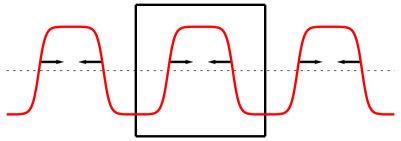
Figure 2: Kink-antikink initialisation procedure.

Finally, the use of (anti)periodic boundary conditions in a finite volume introduces a small mismatch in the derivative of the field at the boundaries, especially if the kink and antikink are close to them. We therefore use the initialization setup sketched in Fig. 2: we take several configurations in several adjacent lattices and use the resulting configuration in one of them,

$$\phi_{K\overline{K}}(x,t)\Bigl{|}_{t=0,a_{0}}=-v+\\ \begin{aligned} v\sum_{n=-N}^{N}\biggl{\{}&\tanh\Bigl{[}\gamma\frac{m}{2}(x+[x_{0}-ut]+n\cdot L)\Bigr{]}\\ -&\tanh\Bigl{[}\gamma\frac{m}{2}(x-[x_{0}-ut]+n\cdot L)\Bigr{]}\biggr{\}},\end{aligned}$$ (17)

where $N$ is typically around $8$.

III Hartree kinks at rest

Although interesting in itself the classical theory is not the full story and it is therefore important to study quantized kink solutions. In order to study dynamical processes, such as collisions, one has to use approximation schemes, which are nonperturbative, real-time and which can handle inhomogeneous configurations. For this purpose the inhomogeneous Hartree approximation as studied in Ref. Sallé et al. (2001) and Sallé et al. (2002) should be particularly appropriate, being a nonperturbative semiclassical approximation scheme.

III.1 Initial condition

Unlike in the classical theory, we cannot use the Bogomol’nyi argument to derive a static soliton solution to the Hartree equations (4c). However, if the coupling is not too large, or more precisely, if the two vacua are well separated and the barrier between them is high, the quantum corrections will be relatively small. Furthermore, away from the physical position of the kink, the field resides in one of the vacua, where an exact solution of the Hartree equations is known. Therefore using the classical kink solution as initial condition for the mean field, while using the free field plane wave solutions for the mode functions will be close to a Hartree kink solution, provided the coupling is not too close to the phase transition, i.e., the vacuum expectation value $v$ is (substantially) larger than $1$. After the configuration has evolved, using the Hartree equations of motion, from such an initial condition, it will, at least for a while, oscillate around the actual stationary solution.

A way to improve on this initial condition is to add a damping term

$$-\Gamma\partial_{t}\phi$$ (18)

to the right hand side of the mean field equation (4a) and evolve from the aforementioned initial condition to obtain an approximately stationary solution, which can then be used as a new initial condition. We will discuss this setup further in Sec. IV, when considering colliding kinks. In Sec. III.3 we will use a damping term to determine the quantum kink mass.

Another possibility would be to start with the initial conditions as proposed in Ref. Boyanovsky et al. (1998). However, these still are not stationary under the equations of motion and the advantage is therefore only minor, so we choose to use the simpler vacuum mode functions.

The numerical results presented in the next sections are all obtained using the simple initial condition, with mode functions of free field form and Eq. (17) for the mean field.

III.2 Numerical results: Static kink decay

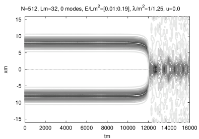
(a) Classical, $\lambda/m^{2}=1/1.25$. For clarity the $x$-coordinate is shifted over $L/2$ through the periodic boundary conditions.

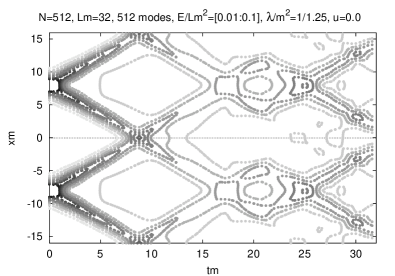
(b) Hartree, $\lambda/m^{2}=1/1.25$.

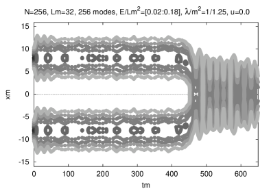
(c) Hartree, $\lambda/m^{2}=1/1.25$, with damping $\Gamma=0.4m$ till $tm=15$. Plotted energy is mean field only.

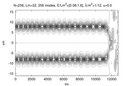
(d) Hartree, $\lambda/m^{2}=1/12$.

Figure 3: Energy density contour plot for kink-antikink annihilation from rest, for different couplings, classical and Hartree. All plots, except 3(c), show total energy density. The vertical energy density range is chosen such as to emphasize the deviation from vacuum which in some of the plots will cut-off the peak at the center of the kink.

In this subsection we are discussing the evolution of a kink-antikink configuration, initially at rest at a maximum distance in the periodic volume. A comparison will be made between Hartree and classical dynamics, using identical initial conditions, in the sense that the mean field in the Hartree simulation is equal to the field in the classical simulation. Hartree simulations at small and large coupling will also be compared. In all cases the same physical volume will be used. Finally the effect of damping on the lifetime of the kink-antikink pair is discussed. The combined results are shown in Fig. 3, in the form of contour plots of the energy density for the 4 different simulations. We have made plots of the energy density instead of the (mean) field, as they show the position of the kink more clearly.

Fig. 3(a) shows a classical simulation at the strong coupling $\lambda/m^{2}=1/1.25$. Fig. 3(b) shows the same simulation, using Hartree dynamics. Fig. 3(c) shows the same Hartree simulation, with a damping $\Gamma=0.4m$ switched on during $tm\leq 15$. Finally Fig. 3(d) shows the result for a Hartree simulation at a weaker coupling $\lambda/m^{2}=1/12$, without a damping term in the equations of motion.

A comparison of classical and Hartree dynamics, Figs. 3(a) and 3(b), respectively, shows an enormous difference in annihilation time between them. The high instability of the Hartree kink antikink pair is caused by the fact that at this strong coupling, the average energy density $e/m^{2}=0.025$ is higher than the potential barrier $\Delta e/m^{2}=0.019$ between the three local minima (remember that the Hartree approximation incorrectly predicts a first order phase transition instead of a crossover), so by exciting particles and spreading the energy the barrier effectively disappears. The fact that we do not use an actual stationary solution to the equations of motion (4c) therefore causes the $K\bar{K}$ pair to evaporate very quickly. It is important to mention that, although it seems from Fig. 3(b) that the kink and antikink each split into two, this is not actually the case. By making an animation of the mean field, we found that it just “contracts” over the barrier, thereby annihilating both kink and antikink. In this process some energy is send off in opposite directions, but this cannot be seen as kink-antikink pairs.

It is also interesting to note that forming a Bose Einstein distribution with the same average energy density would have an inverse temperature $\beta m=3.5$, just below the phase transition at which the three minima become degenerate. Combined with the low barrier this makes it profitable for the configuration to disintegrate, in order to lower the gradient energy, and settle down in the symmetric minimum.

Comparing the Hartree results in Figs. 3(b) and 3(c) confirms the above interpretation. By damping the equations of motion we establish two things. We make the configuration closer to a truly stationary one, thus making it more difficult to excite particles, and by lowering the average energy density the corresponding Bose Einstein temperature moves away from the phase transition point.

After the damping is switched off at $tm=15$, the kink-antikink pair survives until $tm\approx 450$. Switching off the damping at a later instant increases the survival time: using $tm=40$ instead of $tm=15$ results in a survival time of $tm\approx 500$, i.e., the survival time increases by $50$ due to an increase in “switch-off time” of $25$. When we do not switch off the damping, the pair survives until at least $tm=2000$. We have not simulated this system longer, but we do not think it will ever decay.

We also checked the influence of the precise value of the damping constant $\Gamma$, by making additional simulations at $\Gamma=0.2m$ and $\Gamma=0.8m$. At the smaller value, $\Gamma=0.2m$, the pair survival time decreases slightly, $\Delta tm=-20$, at a larger damping, $\Gamma=0.8m$, the survival time increases by only $\Delta tm=+2$. Apparently, using a damping constant $\Gamma=0.2m$ until $tm=15$ already removes most of the fluctuations around the stationary configuration. However, the remaining configuration is still much less stable than its classical counterpart. This is confirmed by a comparison of the total energy density with the depicted mean field energy density: it turns out that the total energy density is much smoother than that of the mean field. Apparently the modes in part cancel out the kink-antikink inhomogeneities, thus facilitating the final annihilation of the pair.

There is an important subtlety with the implementation of the damping term. Since it is far from easy to add such a term to the equations of motion of the mode functions – even in the vacuum their unrenormalized kinetic term is not vanishing – we only implement one in the mean field equation of motion. However, this makes the actual decrease of the energy density much slower, as it involves the transfer of energy from the modes to the mean field. We have seen in the simulations that there are basically two timescales, a rapid initial decrease, approximately with the damping rate expected, after which most of the kinetic energy of the mean field has disappeared, followed by a very slow decrease, draining the energy of the modes. When switching off the damping after the initial stage, as we have done in the simulation of Fig. 3(c), the kinetic energy of the mean field starts growing again, be it slowly, and a new energy equilibrium is established. When the damping is not switched off, the system evolves exponentially slowly towards its final state. We will come back to this in the next section, in the study of the Hartree kink mass.

By comparing Fig. 3(b) at $\lambda/m^{2}=1/1.25$ with Fig. 3(d) at $\lambda/m^{2}=1/12$, we see that at the weaker coupling, the use of the classical kink form for the mean field and plane waves for the modes is much closer to a stationary solution, even without damping. The configuration is oscillating around an approximately stable solution for an extensive period of time, before annihilation. By comparing Fig. 3(d) with the damped strong coupling result Fig. 3(c), we see that the kink is broader at the stronger coupling, due to a change in the effective potential caused by the quantum modes (we also checked this broadening directly in a plot of the mean field). Classically the width only depends on the mass $m$, which by construction is the same for both couplings. This change of width gives another interpretation for the fact that at larger coupling, the kink-antikink configuration is less stable: relative to their own size, the separation is smaller.

As a final remark, it is important to note that the annihilation in Figs. 3(b)–3(d) is not due to tunnelling but is an “over the barrier” annihilation. In Fig. 3(a) this is clear as it is a purely classical simulation, but one could suspect that the much shorter decay time in the quantum Hartree simulations is due to tunnelling. However, in all cases, including the classical, the decay is due to the attractive force between the kink and the antikink. The attractive potential falls off exponentially with the separation, and small deviations from the stationary state only lead to decay after very long times. At strong coupling the deviations are larger and, as we have seen, in the Hartree simulations the effective relative distance becomes smaller due to the broader kinks. In all runs in Figs. 3, except Fig. 3(b), the kink and antikink are moving towards each other before the decay, due to this attractive force, until they bounce and annihilate. After that the mean field ends up in one of the two “broken minima”. In Fig. 3(b), the barrier is so low that the field just moves over it and decays in that way. In this run, the field oscillates around the “symmetric minimum” after the decay, as already discussed before.

III.3 Numerical results: Kink mass

In this subsection we will discuss the kink mass, the energy of the static solitonic configuration. Classically it is given by Eq. (15). In the full theory this expression needs corrections. The first corrections were found by Dashen et al.Dashen et al. (1974), see also Rajaraman Rajaraman (1982), and more recently by Alonso Izquierdo et al.Alonso Izquierdo et al. (2002). A numerical study was done in Ref. Weidig (1999). The result is obtained using a semiclassical perturbative expansion around the classical kink solution. The kink mass is then given by the lowest energy level. This mass has to be renormalized and the net result is

$$M_{\text{kink}}=\frac{m^{3}}{3\lambda}+m\Bigl{(}\frac{\sqrt{3}}{12}-\frac{3}{2\pi}\Bigr{)}+\mathcal{O}(\lambda).$$ (19)

A partial calculation of the order $\lambda$ correction can be found in Ref. de Vega (1976). In this reference and independently also in Ref. Verwaest (1977) a full calculation is done for the order $\lambda$ correction of the kink mass in the sine-Gordon model.

More recently lattice Monte Carlo studies of the kink mass have been carried out Ciria and Tarancón (1994); Ardekani and Williams (1999). In these papers two methods of calculating the kink mass were used: first using the fluctuation-fluctuation 2-point function $\langle\mu(t)\mu(0)\rangle$ introduced in Refs. Kadanoff (1969); Kadanoff and Ceva (1971), which in imaginary time should decay as $\exp(-M_{\text{kink}}t)$. The second uses the difference in the ground state energy when periodic or antiperiodic boundary conditions are used. Both studies focus on a range of parameters, where $\lambda a^{2}$ and $-\mu_{0}^{2}a^{2}$ are of order unity, i.e., at large lattice distances.

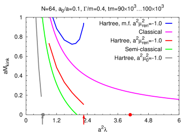
(a) $a^{2}\mu^{2}=-1.0$.

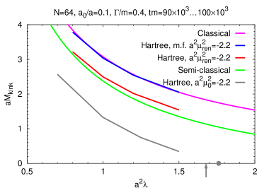
(b) $a^{2}\mu^{2}=-2.2$.

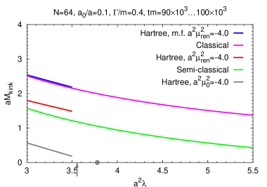
(c) $a^{2}\mu^{2}=-4.0$.

Figure 4: Comparison of classical, semiclassical (one loop) and Hartree results. The Hartree results are plotted for constant renormalized $\mu_{\text{ren}}^{2}$ and unrenormalized $\mu_{0}^{2}$. Also see the text.

Very recently, Bergner and Bettencourt Bergner and Bettencourt (2003) studied the kink mass in the Hartree approximation. Their equations are derived from a 2PI effective action, but applying the Hartree approximation to it results in the same equations of motion we are considering here. Using a numerical relaxation method they have obtained the Hartree kink mass at $\lambda/m^{2}=0.5$ to be $0.4691$ (translated in our units), which is about $70\%$ of the classical value. We have reproduced their value using antiperiodic boundary conditions and a damping term (18) in the mean field equation of motion. On a lattice with $N=64$ and $Lm=16$, $a/a_{0}=10$ using a damping coefficient $\Gamma/m=0.4$ we find at a time $tm=9\times 10^{3}-10\times 10^{3}$ a value $M_{\text{kink}}/m=0.47$. Doubling the lattice size or decreasing the temporal lattice distance increases this value by about $1\%$, while increasing the simulation time with an order of magnitude decreases it by about $2\%$. Unlike Bergner and Bettencourt we have not fixed the center of the kink, but the fact that the mass turns out equal shows that the zero mode can have at most a small effect, in agreement with Ref. Ardekani and Williams (1999).

In order to make a detailed comparison with the full theory, i.e., the Monte Carlo data of Refs. Ciria and Tarancón (1994); Ardekani and Williams (1999), we have done simulations for a range of parameters. The results are shown in Fig. 4. We show results for constant renormalized $\mu_{\text{ren}}^{2}$ as well as constant unrenormalized $\mu_{0}^{2}$. For the constant $\mu_{\text{ren}}^{2}$ we also show separately the mean field contribution, defined as in Eq. (16), Ref. Sallé and Smit (2003). The data in Refs. Ciria and Tarancón (1994); Ardekani and Williams (1999) is shown as a function of the unrenormalized $\mu_{0}^{2}$, in order to study the renormalization effects. However, to make a meaningful comparison with the classical and semiclassical 1-loop results, it seems more proper to compare at constant $\mu_{\text{ren}}^{2}$. The arrows in the plots show the zero temperature phase transition point, at which the three minima become degenerate, calculated using the static effective potential, cf. Ref. Sallé et al. (2001). The dots indicate the point at which the “broken” minima vanish altogether. In order to make the comparison with the Monte Carlo data easier, lattice units have been used. Most simulations where done with $N=64$, $a_{0}/a=0.1$ with a damping term $\Gamma/m=0.4$ while the energy was measured at $tm\approx 100\times 10^{3}$. We have checked for lattice artefacts (the influence of $N$ and $a_{0}/a$), their combined error is not larger than about $1\%$. Also the effects of the precise value of the damping term and time at which the mass is measured are small and of the same order of magnitude as that of lattice artefacts.

We see that for all renormalized masses, the Hartree results are between the classical and semiclassical values. Using the unrenormalized mass as the parameter to compare with, the Hartree results are much lower than the semiclassical values. Comparing these with Figs. 4–6 of Ref. Ardekani and Williams (1999) we find that the Monte Carlo results are above the Hartree results. Note that the semiclassical line in Fig. 6 of Ref. Ardekani and Williams (1999) is approximately $0.3$ too high. For the two higher values of $|\mu_{\text{ren}}^{2}|$, where the data taken is further away from the first order phase transition, the mean field contribution is almost equal to the classical value. The difference between the Hartree and classical kink mass only comes from the modes. For the lower $a^{2}|\mu_{\text{ren}}^{2}|=1.0$ the “mean field mass” behaves very interestingly. We see that, coming from below, it goes up again near the phase transition. This is caused by the emergence of the symmetric minimum. More data would be needed to study the precise behaviour at the phase transition, but from its definition, Eq. (16a) in Ref. Sallé and Smit (2003), it seems it only goes up a final amount, due to this symmetric minimum and the change in the effective potential. It is also not clear to us at this stage whether it is only an artefact of the way we split the total energy in a mean field and mode contribution or is an actual physical phenomenon.

Finally, we have measured the mass at a coupling $\lambda/m^{2}=1/1.25$, used for example in Figs. 3(b) and 3(c), using $Lm=16$, $N=64$ at a time $tm=20\times 10^{3}$. In principle we could find the value also in Fig. 4(a), but those data where obtained a large lattice distance and a separate test is useful. The result is $M_{\text{kink}}/m=0.22$, or $54\%$ of the classical value $0.42$. This value for the kink mass is consistent with Fig. 4(a), showing that we are indeed in the scaling region, as claimed by Ref. Ardekani and Williams (1999) (the same is also found for the weaker coupling $\lambda/m^{2}=0.5$, considered in Ref. Bergner and Bettencourt (2003)). The semiclassical value (19) from Ref. Dashen et al. (1974) gives a value $0.08$, about $1/5$ of the classical value. Note that at $\lambda/m^{2}\approx 1$ the semiclassical approximation breaks down, showing up by a change of sign in the kink mass, the order $\lambda^{0}$ correction becomes equal to the leading $\lambda^{-1}$ term. In the Hartree approximation we can in principle continue till $\lambda/m^{2}\approx 1.2$, where the zero temperature phase transition occurs.

IV Moving Hartree kinks

IV.1 Initial condition

In order to describe kink-antikink collisions, it is necessary to have a description of a moving Hartree kink as well. In the full quantum theory this poses a difficult problem, since we do not know how to Lorentz transform the “quantum cloud” surrounding the kink. In the Hartree approximation we are saved by the fact that the field is completely expressed in terms of ordinary functions of $x$ and $t$, and we can find a moving kink by performing a simple Lorentz transformation:

$$f(x,t)\to f^{\prime}(x,t)=f(\gamma[x-ut],\gamma[t-ux]),$$ (20)

both on the mode functions and the mean field.

However, there are still a number of difficulties with finding a proper initial condition for a kink-antikink pair, moving toward each other. First of all, from Eq. (20) it follows that we need the mode functions on a backwards space-time line, while we do not know them in analytic form, only from numerical simulations. For the classical kink solution this problem does not exist, since it is not only stationary, but also static and known analytically. Second, we have to boost the kink and antikink, with their respective mode-functions, in opposite directions. This means that they have to be combined in a nontrivial way in the middle, they “shift into each other”. It also means that we have to double the density of mode functions in $k$-space, since the physical space doubles (the best one can do is determine the mode functions for a single kink). We have to decide how to do this in a consistent way. Finally there is the problem that the boosted coordinates $\gamma(x-ut)$ and $\gamma(t-ux)$ will in general not fall onto space-time lattice points in the unboosted frame or vice versa.

In order to circumvent these problems, we will just use the vacuum form as initial conditions for the mode functions. Since the vacuum is invariant under Lorentz transformations, we can use the same mode functions in a boosted frame. As mentioned before, the mode functions will be close to the vacuum form, if the vacuum expectation value $v$ is large. Furthermore by boosting the kink solutions we reduce the width of the kinks. However, in the center of mass frame, we keep the lattice size the same thus effectively increasing the relative distance between them. This leads to much more stable solutions, which is even further enhanced by the time dilatation.

Before we proceed we will outline a set of solutions for the aforementioned problems, which will yield a very accurate, boosted, Hartree kink-antikink solution and will therefore also be usable at strong coupling and low speeds. In the simulations we will in general, for simplicity, only use the vacuum form mode functions.

The way to solve the stability problem of a (single) kink is to use damped equations of motion, as we already used in the preceding subsections, especially in combination with antiperiodic boundary conditions on the mean field to make the kink absolutely stable. The damping will give us stationary, but time-dependent solutions for the mode functions in the background of a kink, which subsequently can be Lorentz boosted.

The problem of the boosted coordinates not resulting from discrete lattice points in the unboosted coordinate can be adequately solved by linear interpolation, provided the lattice distance is not too large. The related matching problem is not a real problem: we have to match the two functions at two consecutive time steps and when they approach each other with speed $u$, they shift into each other over a distance $ua_{0}\ll a$, i.e., the mismatch is less than a lattice distance and the linear interpolation automatically solves the problem.

The remaining problem is to combine the two sets of mode functions, of the separate kink and antikink configurations, into one set which is twice as large. One possible solution is to determine both kink and antikink in a volume that already has the size of the combined configuration and then use an averaging procedure to combine the modes. This has the disadvantage that oscillatory functions with different phases are added. Another way, which we suggest, is to determine the two configurations in their original volume and combine them afterwards into one set in the double volume. When using periodic mode functions, it follows from the antiperiodicity of the mean field that at all times

$$f_{k}(x,t)=f_{-k}(L-x,t),$$ (21)

provided this relation holds at $t=0$ and $t=a_{0}$, a condition which is true for the plane wave initial conditions we use. Note that at later times the $k$ label is no longer equal to the Fourier label, for which the relation holds trivially. We can therefore combine each mode function $f_{k}$ with either itself or with $f_{-k}$, since both combinations yield continuous functions. The derivative will in general be discontinuous by changing sign, possibly causing trouble in the equation of motion. However, the energy density will be finite and even continuous, as it only depends on the square of the first derivative, which is continuous.

We end this subsection summarizing the above steps one could follow to obtain a better initial state for a colliding kink-antikink pair. First, using antiperiodic boundary conditions for the mean field and a damping term $-\Gamma\partial_{t}\phi$, one evolves the Hartree equations, starting from a classical kink with free field mode functions. One thus obtains a stationary Hartree solution for a single kink, but has to keep track of the modes and mean field on a backward space-time line. Then one constructs the mean field from the kink and its mirror image. The modes are constructed by combining $f_{k}(x,t)$ with itself and with $f_{-k}(x,t)=f_{k}(L-x,t)$, thereby doubling their number,

$$f_{k,1}(x,t) =\begin{cases}f_{k}(x,t),&0\leq x\leq L,\\ f_{k}(x-L,t),&L\leq x\leq 2L,\end{cases}$$ (22a)

$$f_{k,2}(x,t) =\begin{cases}f_{k}(x,t),&0\leq x\leq L,\\ f_{-k}(x-L,t),&L\leq x\leq 2L.\end{cases}$$ (22b)

The latter, symmetric, combination can lead to functions in which the second derivative diverges as $1/a$: the energy density, depending only on the square of the first derivative, is finite and continuous in the continuum limit, however it might cause problems in the equations of motion.

IV.2 Numerical results: Thermalization from colliding kink-antikinks

We start the discussion of our numerical results with the thermalization properties of a colliding kink-antikink pair, using the defining relation (10) for the particle number $n_{k}$. We used a small coupling, $\lambda/m^{2}=1/12$, in a volume $Lm=32$ at a speed for which $\gamma=2$. The classical kink mass at this coupling is $M_{\text{kink}}/m=4$. Since we initialize the mean field as a classical kink and the modes in the vacuum, the initial energy density is $E/Lm^{2}=2\cdot(4+4)/32=0.5$. At this energy density and coupling we found, in Ref. Sallé et al. (2001), both in dynamical simulations and an effective potential calculation, a temperature $T/m\approx 1.0$.

In order to enable us to correctly interpret the result, we also measured the “particle number” at $tm=0$. Of course at this time the system is so far from equilibrium that we cannot interpret the result as quasiparticles, but it does give an idea of the energy distribution as a function of $k$. The result is plotted in Fig. 5. The similarity with a Bose-Einstein distribution is remarkable and we have to be careful in interpreting the results at later times. One of the indications, that it is not a truly thermal distribution, is its very low “temperature”: at an energy density $E/Lm^{2}=0.5$ we expect to find a temperature around $T/m=1.0$, while Fig. 5 seems to indicate a value which is almost a factor of 3 smaller. Furthermore, the particle number mainly comes from the even modes, as a result of the symmetric initial condition.

Fig. 6 shows the actual particle number, at later times, when the kink-antikink have already annihilated. Then, we do find a temperature around $1$, conform the results of Ref. Sallé et al. (2001). As a comparison we also plotted, in the same figure, the result obtained in that paper using a flat ensemble simulation. It clearly shows that the temperatures are equal: $T$ is uniquely determined by the coupling and energy, not by the initial condition. The initial condition still has an influence in determining which modes have thermalized. We see that starting from an annihilating $K\overline{K}$ actually allows the system to thermalize faster, as it has a more favourable energy distribution, cf. Fig 5. However, the $K\overline{K}$ initial condition has a delta function initial density matrix, which is not very suitable for our Hartree ensemble approximation: we do not reduce the statistical errors by averaging over multiple initial conditions.

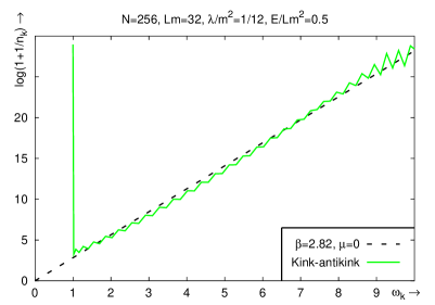
Figure 5: Initial form ($tm=0$) of the particle distribution for a Hartree kink-antikink collision. The initial form already seems close to a Bose-Einstein distribution.

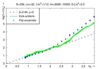
Figure 6: Late time form of the particle distribution for a Hartree kink-antikink collision. $tm\approx 10000$, after annihilation.

Having showed that this initial condition also leads to an approximately thermal Bose-Einstein distribution after annihilation, we will now leave the thermalization topic and continue with a discussion of the actual collisions.

IV.3 Numerical results: Critical speed

We start this section with a study of classical kink-antikink collisions. An extensive study of this can be found in Ref. Campbell et al. (1983).

Figs. 7 show energy contour plots of Lorentz boosted classical kink-antikink configurations. The results in these plots demonstrate how, at very low incident speed, they just annihilate, while at a certain range of higher speeds, they bounce a few times and then either annihilate or escape again to infinity, at a slightly lower speed. At high enough speeds, when $u$ is larger than a certain $u_{c}$, which has a value between $0.25$ and $0.30$, the pair immediately escapes after the collision, again with a lower speed. Part of the kinetic energy is transferred to an internal vibrational mode of the kink, which can be seen as a wiggling in the contour plots.

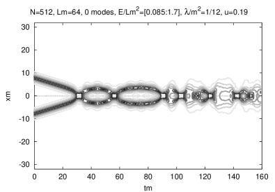
(a) $u_{i}=0.19$ ($\gamma\approx 1.019$).

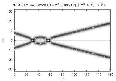
(b) $u_{i}=0.20$ ($\gamma\approx 1.021$).

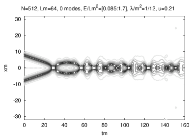
(c) $u_{i}=0.21$ ($\gamma\approx 1.023$).

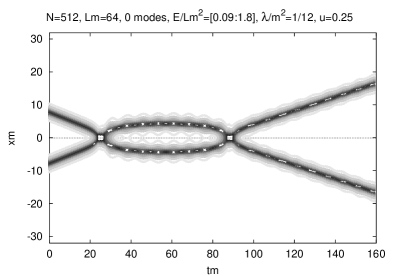
(d) $u_{i}=0.25$ ($\gamma\approx 1.033$).

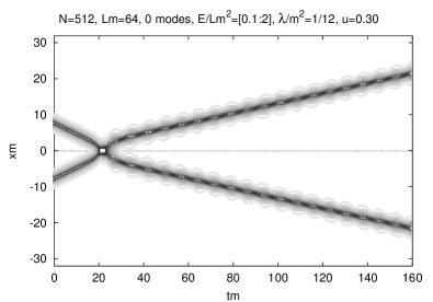
(e) $u_{i}=0.30$ ($\gamma\approx 1.048$).

Figure 7: Colliding classical kink-antikink, $\lambda/m^{2}=1/12$, above and below the critical speed.

These results are consistent with Ref. Campbell et al. (1983) in which a critical speed $u_{c}=0.2598$ is found, above which colliding kinks always bounce back, while below a speed $0.193$, they always annihilate immediately. Between these speeds Ref. Campbell et al. (1983) found reflection and annihilation bands, caused by a resonance between the center of mass motion and the vibrational mode. This was confirmed in Ref. Anninos et al. (1991), also showing that, when zooming in on the bands, their structure behaves fractally. This behaviour could even be reproduced using a collective coordinates approach, reducing the infinite-dimensional system to a two dimensional Hamiltonian one.

Except for Fig. 7(d) all shown results are in accordance with Table I in Ref. Campbell et al. (1983). Since we used different discretizations, etc., and given the very narrow width of the stability bands already found by Ref. Campbell et al. (1983) and the fractal behaviour found in Ref. Anninos et al. (1991), we can certainly expect small differences in the precise position of these bands, explaining the discrepancy. The authors of Ref. Campbell et al. (1983) found that the final speed, for an initial speed above $u_{c}$, satisfies the following relation

$$u_{f}^{2}\propto u_{i}^{2}-u_{c}^{2},$$ (23)

which is consistent with Fig. 7(e), from which we derive a final speed $u_{f}\approx 0.13-0.14$. For $u_{i}=0.30$ relation (23) predicts $u_{f}=0.15$.

It is important to note that although breatherlike states seem to emerge after a collision, truly stable breathers do not exist in the $\lambda\phi^{4}$ theory Segur and Kruskal (1987). However, very long-lived and almost stationary configurations do exist Geicke (1994) as we have shown here again. The radiation causes the energy to decay as $1/\log(t)$, as found analytically by Ref. Segur and Kruskal (1987) and confirmed numerically by Ref. Geicke (1994).

We would like to compare these classical results with the Hartree approximation to see if, in the quantum theory, a critical speed still exists. In the classical theory, one can always use units such that $\mu=\lambda=1$, and one expects a unique critical speed, while in the quantum theory, including the Hartree approximation, this is not the case. However, we will not go much further into the question of the coupling dependence of the critical speed.

(a) $u_{i}=0.700$ ($\gamma\approx 1.400$).

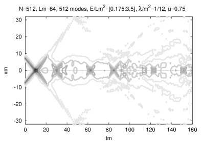
(b) $u_{i}=0.750$ ($\gamma\approx 1.512$).

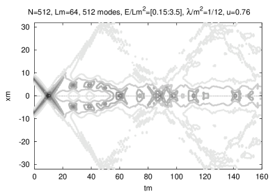
(c) $u_{i}=0.760$ ($\gamma\approx 1.539$).

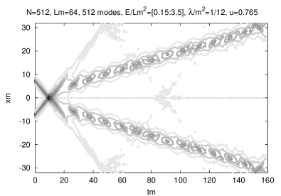
(d) $u_{i}=0.765$ ($\gamma\approx 1.553$).

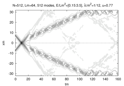
(e) $u_{i}=0.770$ ($\gamma\approx 1.567$).

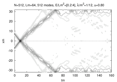
(f) $u_{i}=0.800$ ($\gamma\approx 1.667$).

Figure 8: Colliding Hartree kink-antikink, $\lambda/m^{2}=1/12$, above and below the critical speed.

In Figs. 8 the Hartree results for six different initial speeds are shown. We see that a critical speed does indeed exist, with a value somewhere between $0.760$ and $0.765$, indicating that the quantum kink pair is less stable than its classical counterpart, at least at this coupling. One might think that this instability is caused by the fact that we only have an approximate quantum kink-antikink as initial condition, but as can be seen from Figs. 8, the pair before the collision looks very stable, there is hardly any wiggling, while after the collision the wave packet is dispersing and oscillating and its speed has decreased considerably. The reason for the higher instability is the radiative channel. This probably also causes the fewer number of breather states found: only at an initial speed $u=0.760$, very close to the critical speed, can we recognise an approximate breather state. Bands of stability have not been found and in most simulations in which the pair does not bounce back immediately, the radiation causes them to annihilate.

We also have investigated the functional behaviour of $u_{f}$ as a function of $u_{i}$, to see if it has the same form (23), valid in the classical approximation. The result of several runs at different initial speeds is shown in Fig. 9. We see that close to the critical speed, $u_{f}$ does indeed behave in the same way as in the classical theory,

$$u_{f}^{2}=5.34\left(u_{i}^{2}-u_{c}^{2}\right).$$ (24)

The resulting critical speed $u_{c}$ can be determined very precisely in this way and we obtain $u_{c}=0.760$. Further away from the critical speed the behaviour is not linear in $u_{i}^{2}$, in contrast to the classical result, but the corrections are relatively small.

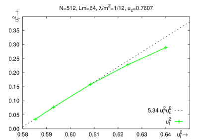
Figure 9: $u_{f}^{2}$ as a function of $u_{i}^{2}$ in the Hartree approximation, showing roughly the same behaviour as in classical theory, but with a $u_{c}=0.7607$.

We have done a few simulations using a stronger coupling $\lambda/m^{2}=1/6$ and they indicate the general behaviour is only slightly different. For example, the critical speed is not very different, it has a value between $0.790$ and $0.795$, from a linear fit of $u_{f}^{2}$ versus $u_{i}^{2}$ we obtain $u_{c}=0.793$ instead of the value $0.7607$ at small coupling. Furthermore at a $u_{i}=0.80$ we find $u_{f}=0.280$, while at $\lambda/m^{2}=1/12$ we found $u_{f}=0.538$. Since $u_{i}=0.80$ is much closer to this value of $u_{c}$, it explains why the value of $u_{f}$ at $u_{i}=0.80$ is a factor of 2 smaller. The prefactor in Eq. (24) is higher at the stronger coupling, around $7$ to $7.5$ instead of the $5.34$, but more data would be needed in order to obtain an accurate answer.

Apart from the factor $3$ larger value of the critical speed, their are other important differences between the classical and Hartree results, Figs. 8 and 7. For example, irrespectively if the pair annihilates or not, a lot of energy is radiated away after the collision in the form of quasiparticles, moving with approximately the speed of light. One might think that the radiation is mainly described by the mode function contribution to the energy density, while the energy density of the surviving kink pair comes from the mean field. However, by checking the different contributions separately we found this is not the case, the kinks are mainly described by the mean field, but also have a contribution from the modes and the radiation is described by both together. Only the total field is a physical quantity describing both the kink-antikink and the radiated particles. Just as only the total two point functions describe the quasiparticles which approximately thermalize.

IV.4 Numerical results: Scaling

As we can describe kink-antikink collisions in a quantum theory, it is interesting to study the possibility of using them as a toy model for heavy ion collisions, such as has been conducted at the SPS, are currently being conducted at RHIC and will later be at the LHC. We therefore look closer at the region just after the actual impact, in collisions with high $\gamma$. In Figs. 10 we show the results of four different simulations, at different $\gamma$ factors and couplings, including one using classical dynamics.

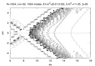
(a) Hartree, $\lambda/m^{2}=1/1.25$, $\gamma=20$ ($u=0.9987$).

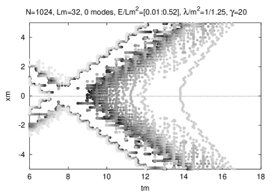
(b) Classical, $\lambda/m^{2}=1/1.25$, $\gamma=20$ ($u=0.9987$).

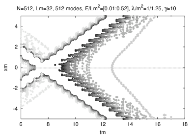
(c) Hartree, $\lambda/m^{2}=1/1.25$, $\gamma=10$ ($u=0.9950$).

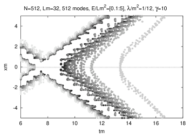
(d) Hartree, $\lambda/m^{2}=1/12$, $\gamma=10$ ($u=0.9950$).

Figure 10: Colliding kink-antikink, period around the collision only.

The plots show a remarkable similarity. In order to investigate this similarity more quantitatively we made time slices shortly after the impact, shown in Figs. 11, at a time $11.5$, the impact itself was at a time $tm\approx 8$ (the determination of the exact time of impact has some complications to which we will return later).

In Fig. 11(a) we see that a different impact velocity only influences the resulting energy density in the emerging kink-antikink, the central region is the same for both speeds. There, the difference in initial speed only shows up in the oscillation wavelength, which scales due to the $\gamma$ factor.

In Fig. 12 we have plotted a similar comparison at smaller coupling, $\lambda/m^{2}=1/12$, as a function of space-time rapidity $\eta=\operatorname{arctanh}(z/t)$ at constant “proper time” $\tau=\sqrt{t^{2}-x^{2}}=10m^{-1}$ ($t=0$ at the collision). Even on the linear vertical scale, the plateau heights are almost identical. It is also striking to see how flat the plateau is, an indication for hydrodynamic scaling. Note that $xm\approx 10\,\sinh(1)\approx 12$ for the edges of the plateau, a large distance compared to the size of the kink, which is much smaller than $1$.

In Fig. 11(b) we show the difference between the two couplings. We have rescaled the energy density with its average over the whole system, in order to facilitate the comparison. Again, the difference is small. At the stronger coupling the energy is slightly more concentrated in the kink-antikink.

Finally in Fig. 11(c) we compare the difference between Hartree and classical dynamics. In both simulations the kink-antikink pair region is very similar. The central region shows some differences, although the total Hartree energy density in this region is very close to the classical energy density. The modes are essential for this, the mean field is more concentrated in the kink-antikink.

To summarize, we have shown that the collisions show scaling behaviour for an extensive range of energies and couplings: they result in approximately the same central region, which is very flat in space-time rapidity. Furthermore at high incident speeds the difference between Hartree and classical is relatively small: classical dynamics can be used in the study of these collisions, giving foundation for its use in the study of heavy ion collisions.

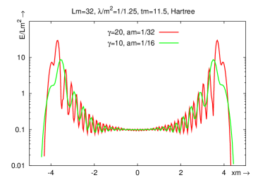
(a) Hartree kink-antikink at $\gamma=20$ and $10$ ($\lambda/m^{2}=1/1.25$).

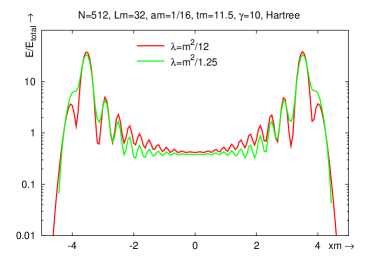
(b) Hartree kink-antikink at $\lambda/m^{2}=1/12$ and $1/1.25$ ($\gamma=10$). The energy density is normalised with the average energy density.

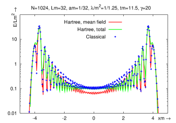
(c) Hartree mean field, Hartree total and classical ($\lambda/m^{2}=1/1.25$, $\gamma=20$).

Figure 11: Comparison of energy density profiles at a time-slice $tm=11.5$, (collision at $tm=8$) for different parameters.

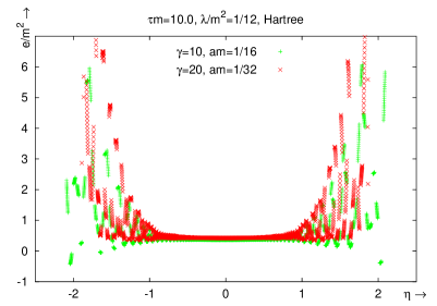
Figure 12: Total energy density in “Bjorken variables” $\tau$ and $\eta$ for two different initial speeds. Note the linear scale.

It is interesting to compare the results obtained here in kink-antikink collisions with what is known about heavy ion collisions. It is already long accepted Bjorken (1983) that the height of the central plateau only weakly depends on the incident speed. Experiments at RHIC, at center of mass energies of $130$ and $200\,GeV$ per nucleus (i.e., $\gamma=130$ and $\gamma=200$, respectively), indicate an increase in particle density of $14\pm 5\%$ Back et al. (2002). At the smaller coupling of $\lambda/m^{2}=1/12$ we find, at a time $tm=3$ after the collision, an increase of only about $3\%$ when increasing from $\gamma=10$ to $\gamma=20$. However, given the very different physical systems, a better match would be a mere coincidence. Longer after the collision, $m\tau=10,\dots,100$, the difference in energy density between the two simulations becomes somewhat larger, as we will see later.

Furthermore, our findings, that only a relatively small fraction of the energy remain in the central region and the concept of a central plateau in space-time rapidity are, at least qualitatively, consistent with real-life heavy ion collisions. A quantitative comparison would not be very meaningful.

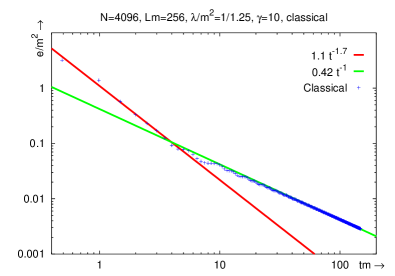
(a) Log-log plot of energy density at $x=0$.

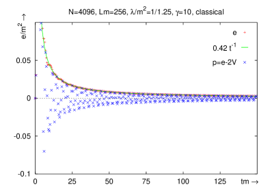
(b) Pressure $p=e-2V$ and energy density. Note that $e$ falls right on top of $p$.

Figure 13: Energy density and pressure in the central region, after a classical kink-antikink collision. At later times, both are consistent with $p=\text{constant}$ and $c_{0}=0$.

A first study of hydrodynamic scaling in a $\phi^{4}$ theory can be found in Ref. Bettencourt et al. (2002). The authors calculate the energy momentum tensor, which in our metric equals

$$T_{\mu\nu}=\partial_{\mu}\phi\partial_{\nu}\phi+\eta_{\mu\nu}\mathcal{L},$$ (25)

in two systems, a colliding kink-antikink and a decaying Gaussian wave packet. For a perfect fluid the energy momentum tensor can be expressed in the energy density and pressure. The assumption of a perfect fluid is valid when collisions can be neglected, as in the (homogeneous) Hartree approximation. For example, the trace of $T_{\mu\nu}$ gives (in $1+1$ dimensions)

$$T_{\mu}^{\mu} =-e+p=-2V,$$ (26a)

$$e =\frac{1}{2}(\partial_{t}\phi)^{2}+\frac{1}{2}(\partial_{x}\phi)^{2}+V,$$ (26b)

$$V =\frac{1}{2}\mu^{2}\phi^{2}+\frac{1}{4}\lambda\phi^{4}+\frac{\mu^{2}}{\lambda}.$$ (26c)

Note that this is a slightly different definition from the one given in Ref. Bettencourt et al. (2002), Eq. (13), as we would like both $T_{00}$ and $T_{11}$ to vanish in the vacuum $\phi=v$. Also note that we just write the classical expressions, the extension to Hartree is straightforward. From Eqs. (26) we find the pressure

$$p=\frac{1}{2}(\partial_{t}\phi)^{2}+\frac{1}{2}(\partial_{x}\phi)^{2}-V.$$ (27)

Using the scaling behaviour one can then, for example, express the speed of sound in the energy density in the center

$$e\propto\tau^{-(1+c_{0}^{2})}\to t^{-(1+c_{0}^{2})}\qquad\text{at $x=0$,}$$ (28)

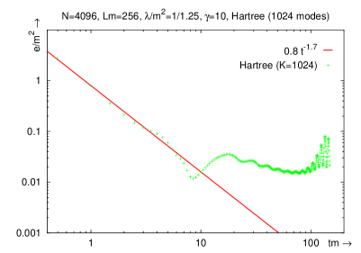
Figure 14: As in Fig. 13(a) but now for a Hartree kink-antikink collision.

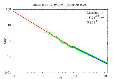
(a) Classical.

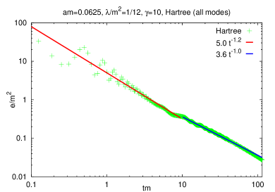
(b) Hartree.

Figure 15: As in Fig. 13(a) and 14 but now for $\lambda/m^{2}=1/12$.

where $\tau=\sqrt{t^{2}-x^{2}}$ is the “proper time” and $c_{0}$ is the speed of sound. For a classical kink-antikink collision at strong coupling $\lambda/m^{2}=1/1.25$ we plotted the central energy density as a function of time (where the time is set to zero at the end of the collision), on a log-log plot in Fig. 13(a) and, on a linear scale, together with the corresponding pressure, in Fig. 13(b). Both from Eqs. (26) and Eqs. (28) we find that shortly after the collision, the pressure in the central region becomes zero, leading to a vanishing speed of sound. This indicates that after this initial stage, the interaction becomes negligible and we just see free expansion, in agreement with the flat central plateau. Initially, however, the system is interacting and there is a non-vanishing speed of sound of about $0.8$. The actual value depends quite strongly on the time origin. We have derived the value to use, from contour plots such as Figs. 10. They show that the kink-antikink stay together for a short period of time $\Delta tm\approx 0.5$.

The result obtained from Hartree dynamics is shown in Fig. 14. In this case we can only find a speed of sound in the first stage, resulting in a value very similar to the classical result. The second stage exhibits strange oscillations but no power behaviour. This is caused by the emergence of a “symmetric minimum” at $\phi=0$, already discussed in Sec. III.2. In Figs. 15 we show the results for collisions at the smaller coupling $\lambda/m^{2}=1/12$. Here we see that both classical and Hartree results give an approximately vanishing speed of sound and thus pressure. The initial speed of sound is for both smaller, about a factor of $2$ compared to the strong coupling, which is (qualitatively) consistent with a smaller coupling. The Hartree result, Fig. 15(b), shows small deviations at the latest times, indicating some interaction. At a higher incident speed, $\gamma=20$, the prefactor in the $1/\tau$ decay rises to $4.4$, both for the classical and Hartree simulations. It is interesting to see that this increase is actually very close to the RHIC results as discussed above.

It is difficult to compare our results quantitatively with those of Bettencourt et al. Bettencourt et al. (2002), since their result for the speed of sound was obtained for a disintegrating Gaussian wave packet in the “symmetric phase.” The effective coupling in the “symmetric phase” is much smaller than in the “broken phase” Sallé and Smit (2003) and we have studied only the central region in the wake of a kink-antikink collision, as this is more similar to a heavy ion collision. The free expanding region is not present in the results of Ref. Bettencourt et al. (2002) and the power behaviour is less pronounced. However, the speed of sound in the initial region is very comparable.

V Thermal kink nucleation

In this section we briefly discuss the thermal creation and annihilation properties of the kink-antikink pairs. There is a long history of papers on the subject of thermal nucleation. See, for example, Ref. Currie et al. (1980) and references therein for an analytical study, and for example Refs. Grigoriev and Rubakov (1988); Alford et al. (1992); Alexander and Habib (1993); Alexander et al. (1993); Habib and Lythe (2000) for numerical studies. Very recently Ref. Holzwarth (2003) has made a study in a heavy ion collision context, calculating classically the multiplicities of $K\bar{K}$ in an expanding Bjorken frame, starting from a Boltzmann distribution.

All these (numerical) studies so far have only considered the classical nucleation rate. The Hartree ensemble approximation method allows us to study the creation of kink-antikink pairs starting from a thermal Bose-Einstein distribution and to compare the classical and Hartree approximation. One of the problems we are thus faced with is a proper definition of kink number. Since only pairs, with no net kink number can be created, we need an effective kink number definition. The actual winding number will always be $0$ or $1$, depending only on the boundary conditions. Furthermore, in the quantum theory, one might think the kinks will be fully described by the mean field, while the mode functions just describe fluctuations around them. However, as we already noticed before, this split-up cannot be taken so rigorously: the kink number will also be partially described by the modes and a definition based on the ensemble description of our system is needed, as only ensemble averaged quantities are physically meaningful.

In the classical theory, a useful quantity to look at is the following,

$$Q_{\text{class}}=\overline{\phi(x)^{2}}-\overline{\phi(x)}^{2},$$ (29)

where the overline denotes a spatial average over the full lattice size. When a kink-antikink pair is present, this observable will become of the order $v^{2}$. If the coupling is not too small, it will therefore give a reasonable indication for their presence. Note that it cannot distinguish between one or multiple pairs and that it becomes smaller if the pair is not at maximum separation. The advantage is that we can easily extend its definition to the quantum theory

$$Q=\overline{\mbox{$\langle\hat{\phi}(x)\hat{\phi}(x)\rangle$}}-\overline{\mbox{$\langle\hat{\phi}(x)\rangle$}}\;\overline{\mbox{$\langle\hat{\phi}(x)\rangle$}}$$ (30)

and that it can be easily found from $S_{k}$, Eq. (9). It is however UV divergent and should be renormalized by subtracting the vacuum contribution:

$$Q_{\text{ren}}=\frac{1}{L}\sum_{k}\Bigl{(}S_{k}-\frac{1}{2\omega_{k}^{\text{free}}}\Bigr{)}.$$ (31)

We now have a quantum kink indicator, showing if a pair is present and which can be easily compared to the classical theory. This is done in two simulations at $\lambda/m^{2}=1/12$ in a volume $Lm=64$, at an inverse temperature $\beta m=0.563$, just below the thermal phase transition at $\beta m=0.562$. At such a high temperature we expect the highest creation rate. In a volume $Lm=64$, it would follow from Refs. Alexander and Habib (1993); Alexander et al. (1993), that we should find about a half to two kinks per total volume, depending on the counting algorithm. The result for $Q$ is shown in Fig. 16. We can clearly see it is different from zero, showing the presence of kink-antikink pairs. Furthermore, these pairs emerge through the dynamics, initially the number is lower. Finally, although the quantum number is smaller than the classical, it does not go away, while, if we look at the mean fields in different realisations separately, we find the kink-antikinks do seem to disappear in the Hartree approximation. From the $Q$ indicator we conclude that they first are contained in the mean field, while later their description is taken over by the modes, again showing that only the total two-point functions, from the total field, describe the physical quantum field. As an example of their emergence from the dynamics, we plotted, in Fig. 17, the mean field of one of the realisations at 4 different times. Initially the field fluctuates around one of its minima, with a reasonable amount of energy, it then forms a $K\overline{K}$ pair, which subsequently annihilates, while transferring its energy to the quantum modes, as can be seen from the smaller amplitude of the fluctuations. The total two-point function still describes $K\overline{K}$ pairs, but this cannot be seen from the separate realisations.

VI Conclusion

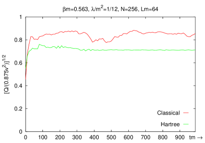
Figure 16: Kink indicator parameter $Q$ from Eq. (31) for classical dynamics (upper plot) and Hartree dynamics (lower plot). Both values are normalised with the value $0.875$, the value of $Q$ for a symmetrically placed kink-antikink pair in a volume $Lm=64$. Of course this value heavily depends on the exact position of the kinks.

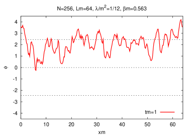
(a) $tm=1$

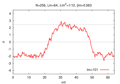
(b) $tm=100$

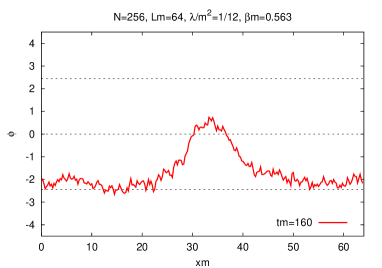
(c) $tm=160$

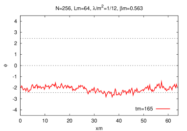
(d) $tm=165$

Figure 17: Thermal kink nucleation and subsequent annihilation in the Hartree approximation. The dotted lines are at the zero temperature “broken” and “symmetric minima” $\pm v(T=0)$ and $0$.

In this paper we looked at the topological defects which can be present in a scalar $\lambda\phi^{4}$ theory: kinks and antikinks. After rederiving the classical solutions, we used both classical and Hartree dynamics in studying their annihilation, both when initially at rest and when boosted. We found that classical kink pairs are much more stable than their Hartree counterparts. Hartree kink pairs at smaller coupling are therefore also more stable than at larger couplings. Although an exact Hartree solution to the equations of motion is not known, by damping the mean field equation, we are able to find an approximate solution. This damping can, especially at larger couplings, prolong the survival time enormously, but is still orders of magnitude shorter than for a classical kink-antikink pair, due to radiation in the form of quantum particles, the quasiparticles discussed in Refs. Sallé et al. (2001, 2002). We suggested an algorithm to find an accurate, numerical and more stable solution for the Hartree equations of motion, but have not yet implemented it.

Using a damped mean field equation of motion we were also able to determine approximately the quantum kink mass. The Hartree approximation seems to give better results than the one-loop semiclassical approximation, especially at larger couplings, where the semiclassical approximation becomes less reliable. The mean field contribution shows a funny increase as a function of coupling, when approaching the phase transition, although the total kink mass behaves regular. It is not yet clear how to interpret this. Damping the equations is not very efficient, as it can only be implemented in the mean field equation, leading to very long relaxation times. We found a rapid short relaxation until a time $tm\approx 10-20$, in which most of the mean field energy is removed, followed by an exponentially slow relaxation in which the energy of the modes is drained indirectly via the mean field. Comparing the Hartree results with Monte Carlo results from Refs. Ciria and Tarancón (1994); Ardekani and Williams (1999) seems to indicate that the Hartree results, although larger than the one-loop semiclassical results, are still too small.

We have shown that a colliding kink-antikink pair, after annihilation, also leads to an approximate thermal Bose-Einstein spectrum, just as a flat initial ensemble. The initial energy distribution has a form which approaches the thermal distribution more easily than the flat ensemble, as used in Ref. Sallé et al. (2001). This makes it possible to recognise the Bose-Einstein distribution already in an early stage. However the statistical errors are larger, since we cannot average over multiple initial conditions. It does show that the result of Ref. Sallé et al. (2001) is rigorous, it does not depend on the specifics of the initial ensemble.

In the study of kink collisions, we found once more that the classical kinks are much more stable: for the classical dynamics, we reproduced the results of Ref. Campbell et al. (1983) on the critical speed and the existence of approximate breather modes. In the Hartree approximation the critical speed is considerably higher and we were not able to find stability bands, i.e., approximate breather solutions. In order to make this result rigorous, many more simulations have to be done, at higher numerical precision, since the radiation makes it difficult to see clearly if a short-lived bound state, or breather, has emerged. The precise dependence on the coupling is also still an open question. In the classical theory the dimensionless critical speed is independent of $\lambda$ as the action can be rewritten in a way that $\mu=\lambda=1$, while in the quantum theory, this is not possible.

We compared some of the results from these kink-antikink collisions with the heavy ion collisions such as are currently carried out at the RHIC in Brookhaven and in the future at the LHC at CERN in Genève. Although the scalar $\phi^{4}$ theory is too simple to serve as a toy model for this, it is interesting to see that we can certainly compare some of the ingredients. The kinks then describe the colliding hadrons or ions, while the quasiparticles describe the formed “plasma”. After the collision, most of the energy remains in the receding kink-antikink, while the resulting field shows a central plateau, flat in space-time rapidity, indicating hydrodynamic scaling. Its height only weakly depends on the initial speed of the kinks and scales with the coupling in a very straightforward way.

We found that the central region first has a finite speed of sound, of about $0.8$ for $\lambda/m^{2}=1/1.25$ and about $0.4$ for $\lambda/m^{2}=1/12$. After a short while this goes over in a free expansion, with vanishing pressure and speed of sound.

In this aspect the qualitative difference between the Hartree and classical approximations is small. Although it is difficult to compare the two at strong coupling at the later stage, as the Hartree approximation is “haunted” by the “symmetric minimum” at $\phi=0$, at the early stage a meaningful comparison can be made. It shows very similar results between the Hartree and classical approximations. At smaller coupling the two are very similar even during the later stage, the Hartree result shows somewhat more interaction at times around $50-100$ and related to that a somewhat smaller energy density.

It would be interesting to have some handle on the error induced by the first order phase transition predicted by the Hartree approximation. Although the lack of a systematic expansion parameter in this approximation makes it difficult to make a quantitative estimate, the above results seem to indicate a qualitatively small influence, even at strong coupling, as long as the field is not moving too close to the artificial “symmetric minimum”. However, at the later stage in the strong coupling simulation of Fig. 14, the field is actually fluctuating around this artificial minimum at $\phi=0$ and the results can no longer be trusted. Similarly, it is not expected that the Hartree approximation can accurately describe the dynamics of going through the phase transition, see Ref. Sallé et al. (2002).

In Ref. Bettencourt et al. (2002) the Hartree “plasma” was also found to behave as a “relativistic plasma,” with speed of sound close to $1$, similar to what we found for $tm\lesssim 8$. However the result in Bettencourt et al. (2002) was obtained from a disintegrating Gaussian wave packet in the “symmetric phase,” in which the effective coupling is much smallerSallé and Smit (2003), instead of a colliding kink-antikink in the “broken phase.” No free expanding phase was found in that reference.

Finally, we have briefly looked at the connection between a thermal Bose-Einstein distribution and the creation and annihilation of kinks in the system. We found that one should only consider the complete field in the description of kinks, not just the mean field. This means that we have to look at quantum and ensemble averages only; the separate realisations give some impression of what is happening but do not describe the full theory. It is encouraging to see that although the kinks disappear from the mean field, our rough kink indicator does not go to zero, but becomes constant, i.e., the creation and annihilation rates become equal. However, we do find fewer pairs in the Hartree approximation than in the classical theory. This might be related to the higher instability of Hartree kinks, which can radiate quantum particles, in the Hartree description, more energy is carried by radiation than in the classical theory.