QCD perturbation theory at large orders with large renormalization scales in the large $\beta_{0}$ limit.

QCD perturbation theory at large orders with large renormalization scales in the large $\beta_{0}$ limit.

Abstract. We examine the QCD perturbation series at large orders, for different values of the ’large $\beta_{0}$ renormalization scale’. It is found that if we let this scale grow exponentially with the order, the divergent series can be turned into an expansion that converges to the Borel integral, with a certain cut off. In the case of the first IR renormalon at $2/\beta_{0}$, corresponding to a dimension four operator in the operator product expansion, this qualitatively improves the perturbative predictions. Furthermore, our results allow us to establish formulations of the principle of minimal sensitivity and the fastest apparent convergence criterion that result in a convergent expansion.

1 Introduction

It has been known for many years that the QCD perturbation series suffers from factorial divergencies [1]. At the same time, we know that the perturbation theory itself does not tell us the whole story and one needs to consider non-perturbative contributions. Because of the asymptotic freedom, we expect these contributions to become more important for lower energies. This is confirmed by the operator product expansion (OPE) [2], the general framework that is used to parameterize the non-perturbative contributions in several power corrections, corresponding to several condensates [3]. In fact, one can show that for one source of divergencies in the perturbation series, the so called IR renormalons, there exists a one to one correspondence with these condensates [4, 5]. This is traced back to the Borel insummability of the perturbation series, leaving ambiguities in the definition of its Borel sum, that can be exactly compensated by different values of the (non-perturbative) OPE condensates. Another crucial problem with the Borel sum, is that the Borel integral is expected to diverge at infinity [1]. However, for now we will disregard this problem and assume that the integral converges at infinity, as is the case for several series in the large $\beta_{0}$ limit. This makes it still possible to define a Borel sum, by choosing a certain prescription for the Borel integral. At large energies, the total result for a physical quantity is then supposed to consist of a Borel sum of its perturbation series, combined with some OPE power corrections, originating from certain values of the non-perturbative condensates.

For a large class of observables, the dimension four gluon condensate is the lowest dimension condensate in the OPE . So the validity of the perturbative expansion for a physical quantity, depending on one external momentum $Q$, is intrinsically limited by a $Q^{-4}$ term. However, the divergent perturbation series gives a stronger limit, coming from the first UV renormalon, positioned at $-1/\beta_{0}$ in the Borel plane. (Incidentally, for the definition of the Borel tranform we use in section 2, the first UV renormalon actually lies at -1.) Dealing with the series as an asymptotic series, one concludes that, at the ’best’ order of truncation, the perturbative prediction can be trusted only up to a $Q^{-2}$ term. In [6], the renormalization scale dependence of the $Q^{-2}$ uncertainty was analyzed, in the large $\beta_{0}$ limit of QCD. It was found that for large orders, the size of this term, can be suppressed by increasing the scale, or equivalently, decreasing the coupling constant in the perturbative expansion.

In this paper we will will extend this analysis, by allowing the renormalization scale to vary with the order of truncation. We will show that if one lets $k$ $(\sim\ln\mu^{2})$, grow linearly with the order of truncation $N$, the divergent perturbation series is turned into an expansion that converges to the Borel integral, cut off at $N/k\equiv 1/\chi$, at least if $\chi>1/2$. This allows us to formulate an expansion that converges to the Borel sum up to a term $\propto Q^{-4}$, roughly compatible with the dimension four gluoncondensate.

In section 2, we examine the large order behavior for the expansion of a generic QCD observable with the typical singularity structure in the Borel plane. We arrive at an asymptotic formula (2), describing the large order truncations for general values of $\chi$. This formula is then applied to different toy expansions in section 3. First we consider the hypothetical situation, were one has only UV renormalons, then we include the IR renormalons. Furthermore we will use formula (2) to establish formulations of the principle of minimal sensitivity (PMS) and the fastest apparent convergence criterion (FACC) that lead to a convergent expansion.

2 The ’scale’ dependence at large orders

Let us start by writing the general expression of the series expansion for a physical quantity $\mathcal{R}$, depending on one external scale $Q$,

$$\mathcal{R}(a_{0})=a_{0}(r_{0}+r_{1}a_{0}+r_{2}a_{0}^{2}+\ldots)\,,$$ (1)

with $a_{0}\equiv\beta_{0}\alpha_{s}(Q)$ ($\approx 1/\ln(Q^{2}/\Lambda^{2})$ for large $Q$). We will examine how the expansion behaves, if we reexpand in some new coupling $a(k)$:

$$a(k)=\frac{a_{0}}{1+ka_{0}}\,.$$ (2)

In the large $\beta_{0}$ limit, this variation corresponds to a change in the renormalization scale (RS) $Q\rightarrow Qe^{k/2}$. Of course nothing prevents us from considering the same variation for real QCD expansions; but it then no longer corresponds to a change of the RS.

The truncation $[\mathcal{R}(a_{0})]_{N+1}\equiv a_{0}(r_{0}+r_{1}a_{0}+\ldots+r_{N}a_{0}^{N})$, is conveniently rewritten as a Borel integral:

$$\int_{0}^{\infty}dt\,e^{-\frac{t}{a_{0}}}[F(t)]_{N}\,,$$ (3)

with

$$[F(t)]_{N}\equiv r_{0}+r_{1}t+r_{2}\frac{t^{2}}{2}+\ldots+r_{N}\frac{t^{N}}{N!}\,.$$ (4)

Under the variation (2) the truncated expansion becomes

$$[\mathcal{R}(a(k))]_{N+1}=a(k)[r_{0}(k)+r_{1}(k)a(k)+\ldots+r_{N}(k)a(k)^{N}]=\int_{0}^{\infty}dt\,e^{-\frac{t}{a(k)}}[e^{kt}F(t)]_{N}\,,$$ (5)

with $[e^{kt}F(t)]_{N}$ the obvious generalization of (4). One now generally assumes that the series $r_{0}+r_{1}t+r_{2}t^{2}/2+\ldots$ has a finite (nonzero) radius of convergence, therefore it defines a function $F(t)$, which is analytical around the origin. In fact, it is established, through the use of several techniques, that $F(t)$ has several types of singularities on the real axis [1, 7, 4, 5] at a nonzero distance of the origin: on the negative axis one finds the UV renormalons at the points $-1,-2,\ldots$; on the positive axis there are IR renormalons at the points $(1),2,\ldots$ and instanton-anti instanton singularities at the points $4\beta_{0}\pi,8\beta_{0}\pi,\ldots$. With the number of active flavors being 3-6 ($\beta_{0}=(33-2N_{f})/12\pi$), the singularities near $t=0$ are all of the renormalon type. In the following we will consider the situation described in the introduction, with no IR renormalon at $t=1$.

One can now make use of the Cauchy integral theorem for analytical functions [8], to write $[e^{kt}F(t)]_{N}$ as a contourintegral along the contour $\mathcal{C}_{0}$ around the origin, excluding the point $t$ and the singularities on the real axis (see Figure 1):

$$[e^{kt}F(t)]_{N} = \sum_{n=0}^{N}(e^{kt}F(t))^{(n)}|_{t=0}\frac{t^{n}}{n!}$$ (6)

$$= \sum_{n=0}^{N}\frac{1}{2\pi i}\int_{\mathcal{C}_{0}}\!\!\!dz\,e^{kz}F(z)\frac{t^{n}}{z^{n+1}}$$

$$= \frac{1}{2\pi i}\int_{\mathcal{C}_{0}}\!\!\!dz\,e^{kz}F(z)\frac{1-(\frac{t}{z})^{N+1}}{z-t}$$

$$= -\frac{1}{2\pi i}\int_{\mathcal{C}_{0}}\!\!\!dz\,\frac{e^{kz}F(z)}{z-t}(\frac{t}{z})^{N+1}\,.$$

For the last equality, we used the analyticity of $e^{kz}F(z)/(z-t)$ inside $\mathcal{C}_{0}$.

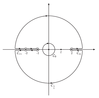
Figure 1: The contour $\mathcal{C}_{0}$, equivalent to the contours $\mathcal{C}_{1/\chi}$, $\mathcal{C}_{UV}$ and $\mathcal{C}_{IR}$, if the residu at $t<1/\chi$ is picked up.

We are interested in the asymptotic behavior of (6); if we put $k=N\chi$, the integrandum can be cast in the form $(\ldots)\times e^{N(\chi z-\ln z)}$, which calls for the saddlepoint technique [8]. So we deform $\mathcal{C}_{0}$ to a circle $\mathcal{C}_{1/\chi}$ with radius $1/\chi$, appropriate for a saddlepoint evaluation. If $t$ is lying inside the circle, one has to pick up the residu $e^{kt}F(t)$, coming from the factor $1/(z-t)$ in the integrandum. As shown in the figure, for $1/\chi$ larger than one (two), one also has to add the contour $\mathcal{C}_{UV}$ ($\mathcal{C}_{IR}$), in order to exclude the singularities and branch lines. For simplicity, we will limit ourselves in the following to pole singularities (without branch lines) at the points $z_{i}=2,3\ldots$ on the positive axis and at the points $z^{\prime}_{i}=-1,-2\ldots$ on the negative axis, arriving at

$$[e^{kt}F(t)]_{N} = \theta(\frac{1}{\chi}-t)e^{kt}F(t)-\frac{1}{2\pi i}t^{N+1}\int_{\mathcal{C}_{1/\chi}}\!\!\!\frac{dz}{z}\,\frac{e^{N(\chi z-\ln z)}}{z-t}F(z)$$

$$+ \sum_{z_{i}}\theta(\frac{1}{\chi}-z_{i})t^{N+1}\frac{e^{N(z_{i}\chi-\ln z_{i})}}{z_{i}(z_{i}-t)}Res_{z=z_{i}}[F(z)]$$

$$+ \sum_{z^{\prime}_{i}}\theta(\frac{1}{\chi}-|z^{\prime}_{i}|)(-1)^{N}t^{N+1}\frac{e^{-N(|z^{\prime}_{i}|\chi+\ln|z^{\prime}_{i}|)}}{z^{\prime}_{i}(z^{\prime}_{i}-t)}Res_{z=z^{\prime}_{i}}[F(z)]\,,$$

with $\theta(x)$ the unit stepfunction.

One can check that the singularities at $t=z_{i}$ of the term $\theta(1/\chi-t)e^{kt}F(t)$, are exactly cancelled by the corresponding terms in the summation over the singularities at the positive axis. Therefore, when performing the $t$ integration of the separate pieces in (2), one can use any prescription, as long as the same prescription is used for every piece. We will use the Cauchy principal value prescription, defined as:

$$PV\!\!\!\int_{0}^{\infty}=\frac{1}{2}(\int_{0}^{\infty+i\epsilon}+\int_{0}^{\infty-i\epsilon})\,.$$ (8)

Before performing the $t$ integration, let us first work out the $z$ integration in the second term of (2). At the saddle point, $z=1/\chi$, one has a a zero derivative for $N(\chi z-\ln z)$. The second derivative is $+N\chi^{2}$, so the path of steepest descent crosses the saddle point orthogonal to the real axis. Furthermore for $z=e^{i\theta}/\chi$,

$$Re(N(\chi z-\ln z))=N(\cos\theta+\ln\chi)\leq N(1+\ln\chi)\,,$$ (9)

thus $\mathcal{C}_{1/\chi}$ is indeed an appropriate choice for the saddle point contour. The integral is conveniently written as:

$$-\frac{1}{2\pi}t^{N+1}\chi e^{N(1+\ln\chi)}\int^{+\pi}_{-\pi}\!\!\!d\theta\,\frac{e^{N(e^{i\theta}-1-i\theta)}}{(1-\chi t)+(e^{i\theta}-1)}\,F\Big{(}\frac{1}{\chi}+\frac{1}{\chi}(e^{i\theta}-1)\Big{)}\,.$$ (10)

With the reparametrization, $\theta=(2/N)^{1/2}x$, this expression is readily expanded in powers of $1/N^{1/2}$. However, one should be cautious for $t\approx 1/\chi$: in that case, the denominator in (10) can not be expanded as

$$\frac{1}{1-\chi t}(1-i\sqrt{\frac{2}{N}}\frac{x}{1-\chi t}+\ldots)\,.$$ (11)

Later on we will see that the dominant contribution of the $t$ integration of (10) in (5), comes exactly from this critical region, therefore we have treated $\Delta\equiv(N/2)^{1/2}(\chi t-1)$, as an order 1 term in the expansion of (10), arriving at:

$$\frac{1}{2\pi}t^{N+1}e^{N(1+\ln\chi)}\chi F(\frac{1}{\chi})\Big{(}f_{0}(\Delta)+\sqrt{\frac{2}{N}}f_{1}(\Delta)+\mathcal{O}(\frac{1}{N})\Big{)}\,,$$ (12)

with

$$f_{0}(\Delta) \equiv i\int^{+\infty}_{-\infty}\!\!dx\frac{e^{-x^{2}}}{x+i\Delta}\,,$$ (13)

$$f_{1}(\Delta) \equiv \int^{+\infty}_{-\infty}\!\!dx\Big{[}\frac{e^{-x^{2}}}{x+i\Delta}\Big{(}\frac{x^{3}}{3}-x\frac{F^{\prime}(\frac{1}{\chi})}{\chi F(\frac{1}{\chi})}\Big{)}+\frac{e^{-x^{2}}}{(x+i\Delta)^{2}}\frac{x^{2}}{2}\Big{]}\,.$$ (14)

One can verify that the odd function $f_{0}(\Delta)$ has a discontinuity at $\Delta=0$ ($t=1/\chi$), $f_{0}(0\pm\epsilon)=\pm\pi$, exactly compensating the discontinuity of the term $\theta(\chi^{-1}-t)e^{kt}F(t)$ in (2). Obviously the discontinuities coming from the other step functions $\theta(\chi^{-1}-z_{i}/|z^{\prime}_{i}|)$ are also compensated by the integration along $\mathcal{C}_{1/\chi}$. In principle one could write

$$F(z)=\prod_{z_{i}}\frac{1}{z-z_{i}}\prod_{z^{\prime}_{i}}\frac{1}{z-z^{\prime}_{i}}\tilde{F}(z)$$ (15)

and incorporate these singularities in the same way as we did for the singularity at $z=t$. This complicates the calculations and only modifies formula (12) for $\chi^{-1}\approx z_{i}/|z^{\prime}_{i}|+\mathcal{O}(1/N^{1/2})$, effectively spreading the discontinuous unit step of $\theta(\chi^{-1}-z_{i}/|z^{\prime}_{i}|)$ in (2), over a region $\chi^{-1}=z_{i}/|z^{\prime}_{i}|\pm\mathcal{O}(1/N^{1/2})$.

We are now ready to perform the $t$ integration of (2) in (5). First, we will consider the integration over the saddle point contribution (12). Notice that the integrandum can be cast in the form $(\ldots)\times e^{N(\ln t-\chi t)}$, with the opposite power of the exponent as for the $z$-integration, so again we have a saddle point at $1/\chi$, but now with the positive axis as the path of steepest descent. With the reparametrization

$$t=\frac{1}{\chi}+\sqrt{\frac{2}{N}}\frac{x}{\chi}\,,$$ (16)

the integral reduces to:

$$\frac{e^{-\frac{1}{\chi a_{0}}}F(\frac{1}{\chi})}{2\pi\chi}\sqrt{\frac{2}{N}}\int^{+\infty}_{-(N/2)^{1/2}}dx\hskip 2.84544pte^{-\frac{1}{\chi a_{0}}\sqrt{\frac{2}{N}}x-\sqrt{2N}x+N\ln(1+\sqrt{\frac{2}{N}}x)}(1+\sqrt{\frac{2}{N}}x)\Big{[}f_{0}(x)+\sqrt{\frac{2}{N}}f_{1}(x)+\mathcal{O}(\frac{1}{N})\Big{]}$$ (17)

$$\approx \frac{e^{-\frac{1}{\chi a_{0}}}F(\frac{1}{\chi})}{\pi\chi}\frac{2}{N}\,\,\int^{+\infty}_{0}dxe^{-x^{2}}\Big{(}f_{0}(x)\big{[}x(1-\frac{1}{\chi a_{0}})+\frac{2}{3}x^{3}\big{]}+f_{1}(x)\Big{)}\,\,\Big{(}1+\mathcal{O}(\frac{1}{N^{1/2}})\Big{)}\,.$$

In the last step we used $f_{0}(-x)=-f_{0}(x)$ and $f_{1}(-x)=f_{1}(x)$. With the introduction of some auxiliary integrations, the integral is calculated exactly, arriving at

$$\frac{1}{N}\frac{e^{-\frac{1}{\chi a_{0}}}}{\chi}\Big{(}(1-\frac{1}{2\chi a_{0}})F(\frac{1}{\chi})-\frac{F^{\prime}(\frac{1}{\chi})}{2\chi}\Big{)}\Big{(}1+\mathcal{O}(\frac{1}{N^{1/2}})\Big{)}\,.$$ (18)

Each term in (2), coming from a renormalon or instanton-anti-instanton at $z_{i}$ ($z^{\prime}_{i}$), contributes a term

$$(\ldots)\times\int^{+\infty}_{0}dt\,\,e^{-t(\frac{1}{a_{0}}+N\chi)}\frac{t^{N+1}}{z_{i}-t}\,$$ (19)

to the $t$ integration (5). With the same reparametrization (16), this is easily expanded (for $1/\chi\approx/\,\,z_{i}$) as:

$$(\ldots)\times e^{-\frac{1}{\chi a_{0}}-N(1+\ln\chi)}\frac{1}{\chi(\chi z_{i}-1)}\sqrt{\frac{2\pi}{N}}\Big{(}1+\mathcal{O}(\frac{1}{N})\Big{)}\,.$$ (20)

After collection of all the terms, we finally arrive at the asymptotic formula for the truncated expansion in $a(k)$ ($k=N\chi$), of an observable $\mathcal{R}(a_{0})$ with Borel transform $F(t)$:

$$[\mathcal{R}(a(k))]_{N+1} = PV\!\!\int^{\frac{1}{\chi}}_{0}dt\,\,e^{-\frac{t}{a_{0}}}F(t)\,+\,\frac{1}{N}\frac{e^{-\frac{1}{\chi a_{0}}}}{\chi}\Big{(}(1-\frac{1}{2\chi a_{0}})F(\frac{1}{\chi})-\frac{F^{\prime}(\frac{1}{\chi})}{2\chi}\Big{)}\Big{(}1+\mathcal{O}(\frac{1}{N^{1/2}})\Big{)}$$

$$+\theta(\frac{1}{\chi}-2)\,e^{-\frac{1}{\chi a_{0}}}Res_{z=2}[F(z)]\,\,\frac{e^{N(2\chi-1-\ln(2\chi))}}{2\chi(2\chi-1)}\sqrt{\frac{2\pi}{N}}\Big{(}1+\mathcal{O}(\frac{1}{N})\Big{)}$$

$$+\theta(\frac{1}{\chi}-1)\,(-1)^{N}e^{-\frac{1}{\chi a_{0}}}Res_{z=-1}[F(z)]\,\,\frac{e^{-N(\chi+1+\ln\chi)}}{\chi(\chi+1)}\sqrt{\frac{2\pi}{N}}\Big{(}1+\mathcal{O}(\frac{1}{N})\Big{)}\,.$$

We have only kept the contribution of the singularity closest to the origin on the positive/negative axis at the point $2/-1$; for all values of $\chi$, this singularity dominates the contributions of the other singularities on the positive/negative axis by a factor $c^{N}$, with $c>1$.

From the discussion on the validity of (12), we know that the asymptotic formula is invalid at the ’steps’ of the $\theta$ functions, $\chi^{-1}=2/-1\pm\mathcal{O}(1/N^{1/2})$.

Also note that the approximations (18) and (20), for the $t$ integration are only valid for $N\gg 1/(\chi a_{0})$. For the relevant values of $\chi$ and $a_{0}$ that we will use later on, this means $N\gg 10$. Therefore, the formula (2) can certainly not be used to examine for instance the NNLO ($N=2$) result. It should be treated as an asymptotic formula, valid for (very) large $N$, assessing the convergence/divergence of the truncations in the limit $N\rightarrow\infty$ for a certain value of $\chi$.

We end this section by quoting the result for the asymptotic formula, in the case of a Borel transform with general singularities. One can verify that the renormalon contributions coming from the $z$ integrations along $\mathcal{C}_{IR}$ and $\mathcal{C}_{UV}$ change to:

$$\theta(\frac{1}{\chi}-2)\,e^{-\frac{1}{\chi a_{0}}}K\frac{\sin(\pi b)}{\pi}\Gamma(-b)\,N^{b}(\frac{1}{2}-\chi)^{b}\frac{e^{N(2\chi-1-\ln(2\chi))}}{2\chi(2\chi-1)}\sqrt{\frac{2\pi}{N}}\Big{(}1+\mathcal{O}(\frac{1}{N})\Big{)}$$ (22)

$$+\theta(\frac{1}{\chi}-1)\,(-1)^{N+1}e^{-\frac{1}{\chi a_{0}}}K^{\prime}\frac{\sin(\pi b^{\prime})}{\pi}\Gamma(-b^{\prime})\,N^{b^{\prime}}(1+\chi)^{b^{\prime}}\,\,\frac{e^{-N(\chi+1+\ln\chi)}}{\chi(\chi+1)}\sqrt{\frac{2\pi}{N}}\Big{(}1+\mathcal{O}(\frac{1}{N})\Big{)}\,,$$

for the singular behavior,

$$F(z)\stackrel{{\scriptstyle z\rightarrow 2}}{{=}}\frac{K}{(2-z)^{1+b}}\,\,,\hskip 28.45274ptF(z) \stackrel{{\scriptstyle z\rightarrow-1}}{{=}} \frac{K^{\prime}}{(1+z)^{1+b^{\prime}}}\,.$$ (23)

Notice that the exponentials, responsible for the large order behavior, have the same arguments as in (2). For $\chi>1/2$, the first two terms in (2) stay the same, and we have essentially the same features for the $\chi$ dependent large order behavior as in the case of pole singularities.

3 Applications

3.1 The UV renormalons

It is instructive to consider first the fictitious case of a series that has no IR renormalons at all. In that case the IR renormalon term in the asymptotic formula (2) should be left out, leaving us with the UV renormalon term as the only possible source of divergence. For $\chi<\chi_{\star}$, with $\chi_{\star}\approx 0.28$ the solution of

$$\chi+1+\ln\chi=0\,,$$ (24)

this UV term diverges exponentially at large orders while it it disappears exponentially for $\chi>\chi_{\star}$. So, only in the latter case the expansion is convergent:

$$[\mathcal{R}(a(N\chi))]_{N+1}\stackrel{{\scriptstyle N\rightarrow\infty}}{{=}}\!\!\int^{\frac{1}{\chi}}_{0}dt\,\,e^{-\frac{t}{a_{0}}}F(t)\,.$$ (25)

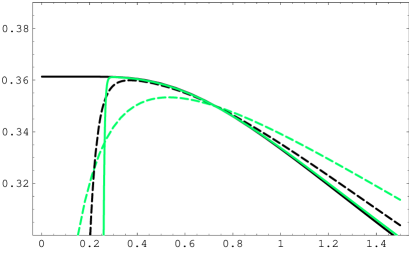
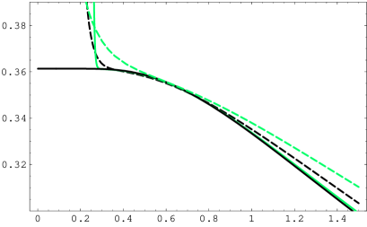
Figure 2: The truncations ${[\mathcal{R}(a(N\chi))]_{N+1}}$, for $N=$3[grey dashed], 9 [dashed], 49[grey] (left) and $N=$4, 10, 50 (right) of the series with Borel transform $F(t)=1/(1+t)$, at $a_{0}=1/2$, as a function of $\chi$. Also plotted: the Borel integral cut off at $1/\chi$ [full line].

This is illustrated in Figure 2, where we plot some approximants $[\mathcal{R}(a(N\chi))]_{N+1}$ as a function of $\chi$, at $a_{0}=1/2$ for the Borel transform $F(t)=1/(1+t)$. This specific model was examined some time ago by Stevenson [9] in the context of the PMS. One clearly observes the behavior predicted by (2): for $\chi>\chi_{\star}$ the expansion converges towards the Borel integral cut off at $1/\chi$, for $\chi<\chi_{\star}$ it diverges. The alternation of the divergence originates from the factor $(-1)^{N}$ in the UV term of the asymptotic formula (2). At the transition region $\chi\approx\chi_{\star}$, one has an extremum for odd orders $N$ and an inflection point for even orders.

From (2) one easily shows for a general $F(t)$ (with no IR renormalons), that for large odd orders an extremum occurs at:

$$\tilde{k}(N)=N\tilde{\chi}\stackrel{{\scriptstyle N\rightarrow\infty}}{{=}}N\chi_{\star}+\frac{\frac{1}{2}\ln N}{1+1/\chi_{\star}}\,,$$ (26)

that is if $Res_{z=-1}[F(z)]/F(1/\chi_{\star})>0$; in the opposite case the extremum occurs for even orders. Furthermore, the substitution of (26) in (2) shows that, although $\tilde{\chi}\rightarrow\chi_{\star}$, the expansion with $k$ at the extremum $\tilde{k}$ still converges:

$$[\mathcal{R}(a(\tilde{k}))]_{N+1} \stackrel{{\scriptstyle N\rightarrow\infty}}{{=}} \!\!\int^{\frac{1}{\chi_{\star}}}_{0}dt\,\,e^{-\frac{t}{a_{0}}}F(t)\,,$$ (27)

in agreement with [9] for $F(t)=1/(1+t)$, also confirmed in figure 2.

With $Res_{z=-1}[F(z)]/F(1/\chi_{\star})>0$ ($<0$), there is no extremum at $k\approx N\chi_{\star}$, for large even (odd) orders. If

$$\frac{1}{a_{0}}>\frac{F^{\prime}(\frac{1}{\chi_{\star}})}{F(\frac{1}{\chi_{\star}})}+2\chi_{\star}\,,$$ (28)

formula (2) instead predicts a zero of the second derivative at:

$$\bar{k}(N)=N\bar{\chi}\stackrel{{\scriptstyle N\rightarrow\infty}}{{=}}N\chi_{\star}+\frac{\frac{3}{2}\ln N}{1+1/\chi_{\star}}\,.$$ (29)

Generally, the condition (28) is fulfilled for $a_{0}$ small enough; for $F(t)=1/(1+t)$, it is met for $a_{0}<2.9$. Again, we have

$$[\mathcal{R}(a(\bar{k}))]_{N+1} \stackrel{{\scriptstyle N\rightarrow\infty}}{{=}} \!\!\int^{\frac{1}{\chi_{\star}}}_{0}dt\,\,e^{-\frac{t}{a_{0}}}F(t)\,,$$ (30)

so the PMS converges to the same value both for odd and even orders, at least if we take $k_{PMS}$ at the extremum/inflection point in the neighborhood of $N\chi_{\star}$. This is in disagreement with the analysis of Stevenson [9] on $F(t)=1/(1+t)$; he predicted the PMS to be biconvergent, with an extra term $\propto e^{-1/(\chi_{\star}a_{0})}$, for even orders.

In the QCD phenomenology one is generally interested in the Borel sum, i.e. the Borel integral cut off at infinity (with a certain prescription in the case of singularities at the positive $t$ axis). Ordinary perturbation theory, with a fixed value of $k$, gives a divergent expansion with an error $\propto e^{-1/a_{0}}\approx Q^{-2}$, at the ’best’ order. For $a_{0}$ not too large, we can estimate

$$\int^{\frac{1}{\chi_{\star}}}_{0}dt\,\,e^{-\frac{t}{a_{0}}}F(t)\approx\int^{\infty}_{0}dt\,\,e^{-\frac{t}{a_{0}}}F(t)+\mathcal{O}(e^{-\frac{1}{\chi_{\star}a_{0}}})\,.$$ (31)

Thus our results imply that, with an appropriate choice of $k$, in the absence of IR renormalons, one can approach the Borel sum much better, up to a correction $\propto Q^{-2/\chi_{\star}}\approx Q^{-7}$. One way to achieve this is to take, for each order, $k$ equal to $N\chi_{\star}$. (It can be checked from (2) that this choice for $k$, still gives a convergent expansion.) Another way is to apply the PMS, as formulated in this subsection.

3.2 Including the IR renormalons

Things change when the IR renormalons come into play. Now, the IR renormalon term in (2) diverges exponentially for $\chi<1/2$; so the expansion only converges for $\chi>1/2$.

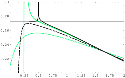
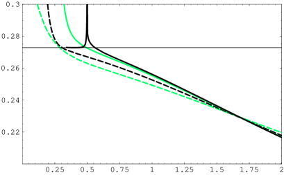
Figure 3: The approximants ${[D(a(N\chi))]_{N+1}}$ of the large $\beta_{0}$ Adler D-function, for $N=$3[grey dashed], 9 [dashed], 49[grey] (left) and $N=$4, 10, 50 (right), at $a_{0}=0.3$, as a function of $\chi$. Also plotted: the Borel integral cut off at $1/\chi$ [full line] and the Borel sum [small full line].

We have performed explicit calculations on the large $\beta_{0}$ limit of the Adler D-function. In this limit the Borel transform is calculated exactly[10]:

$$F_{D}(t)=\frac{32}{3}\frac{1}{2-t}\sum^{\infty}_{p=2}\frac{(-1)^{p}p}{[p^{2}-(1-t)^{2}]^{2}}\,,$$ (32)

with, as expected, singularities for $t=-1,-2,\ldots$ and $t=2,3,\ldots$. Also note that the Borel integral converges at infinity, for $a_{0}>0$. In order to keep the calculation time under control, we have truncated the $p$-summation at $p=100$. In Figure 3, we plot several approximants $[D(a(N\chi))]_{N+1}$, as a function of $\chi$, at $a_{0}=0.3$, together with the Borel integral cut off at $1/\chi$ and the Borel sum. We clearly observe the convergence to the cut Borel integral for $\chi>1/2$ and the divergence for $\chi<1/2$. At the latter region, there is a turnover for odd orders. This occurs when the UV renormalon term starts dominating the IR renormalon term in (2) at $\chi=\ln 2/3\approx 0.23$ for large orders.

Due to the singularity of $F_{D}(t)$ at $t=2$, the cut Borel integral itself also diverges at $\chi\approx 1/2$. (For the sake of clarity, we have only plotted the Borel integral for $\chi>1/3$, thereby omitting all the other divergencies at $\chi=1/3,1/4,\ldots$.) Therefore, the best value for $\chi$, in the sense that the corresponding expansion approaches the Borel sum as close as possible, no longer occurs exactly at the transition between convergence and divergence of the expansion. Instead, it is recommended to take $\chi$ slightly larger than 1/2. If $a_{0}$ is not too large, a good choice will be

$$\tilde{\chi}=1/(2-ca_{0}+\mathcal{O}(a_{0}^{2}))\,,$$ (33)

where $c$ is some positive constant. Indeed, one easily finds that for a general singularity (with $b>-1$)

$$F(t)\stackrel{{\scriptstyle t\rightarrow 2}}{{=}}\frac{K}{(2-t)^{1+b}}\,,$$ (34)

the Borel integral cut at $1/\tilde{\chi}$ is approximated as:

$$\int^{1/\tilde{\chi}}_{0}\!\!\!dt\,e^{-\frac{t}{\alpha_{0}}}F(t)\approx PV\!\!\int^{\infty}_{0}\!\!\!dt\,e^{-\frac{t}{\alpha_{0}}}F(t)+e^{-\frac{2}{a_{0}}}\Big{[}a_{0}^{-b}K[C+\mathcal{O}(a_{0})]+\mathcal{O}(a_{0})\Big{]}[1+\mathcal{O}(e^{-\frac{1}{a_{0}}})]\,,$$ (35)

with $C$ depending on $c$:

$$C=PV\!\!\!\int^{\infty}_{-c}dt\hskip 5.69046pt\frac{e^{-t}}{(-t)^{1+b}}\,.$$ (36)

So we find that, with an appropriate choice for $k$, one can approach the Borel sum up to an error $\propto e^{-2/a_{0}}\propto Q^{-4}$, whereas the ordinary perturbation series, with fixed $k$, gives a minimal error $Q^{-2}$. In addition, if we restrict ourselves in the OPE to the lowest dimension condensate, and to the lowest order term of the Wilsoncoefficient, the $Q^{-4}$ error can be compensated by a redefinition of the condensate. Indeed, with the singular behavior (34), the OPE power correction (proportional to the ambiguity of the Borel integral) to the Borel sum, is written as:

$$Ge^{-\frac{2}{a_{0}}}a_{0}^{-b}K[1+\mathcal{O}(a_{0})]\,,$$ (37)

where $G$ parameterizes the experimentally fitted, non-perturbative condensate. Thus, at leading order in $a_{0}$, the $Q^{-4}$ error (35) is absorbed in the condensate by the replacement $G\rightarrow G^{\prime}=G-C$.

From the second column of Tables 1 and 2, one clearly observes that the approximants with $k=N/(2-2a_{0})$ indeed converge to the Borel integral cut off at $(2-2a_{0})$, for the Adler $D$-function at $a_{0}=0.2$ and $a_{0}=0.4$. This gives an error of $-0.2\%$ and $-8\%$ with respect to the Borel sum for $N\rightarrow\infty$, whereas the divergent series with $k$ fixed at zero, has a minimal error of $5\%$ and $29\%$. Furthermore, there is also a considerable improvement at finite orders.

$N\backslash k$	$0$	$N/(2-2a_{0})$	$k_{PMS}$	$k_{FACC}$
1	-10.77	-7.62	-7.26∗	-7.26∗
2	5.06	-1.31	-3.43	-2.34
3	-5.76	-1.95	-1.80∗	-1.80∗
4	5.39	-1.26	-1.10	-0.93
5	-7.38	-1.12	-0.75∗	-0.75∗
7	-17.6	-0.83	-0.83⋄	-0.41∗
10	150	-0.63	-0.24	-0.22
25	-6$\times 10^{10}$	-0.35	-0.048	-0.0070
50	8$\times 10^{32}$	-0.26	-0.068	-0.034
100	5$\times 10^{91}$	-0.21	-0.088	-0.055
$\infty$	$\pm\infty$	-0.16	-0.12	-0.095

Table 1: Deviations in terms of percentage of the approximants $[D(a(k))]_{N+1}$ for the Adler $D$-function at $a_{0}=0.2$, with respect to the Borel sum, for different values of $k$. For the $N\rightarrow\infty$ limits, we took the cut Borel integral, with the cuts determined according to the text.

$N\backslash k$	$0$	$N/(2-2a_{0})$	$k_{PMS}$	$k_{FACC}$
1	-33.5	-21.7	-21.6∗	-21.6∗
2	28.8	-12.1	/	-15.2
3	-56.3	-12.9	-17.3	-9.83∗
4	119	-11.8	-16.1⋄	-8.73
5	-283	-11.4	-10.8	-4.96∗
7	-2685	-10.7	-11.5⋄	-1.94∗
10	1.8$\times 10^{5}$	-10.0	-14.1	-2.30
25	-2$\times 10^{18}$	-8.89	/	-3.18
50	9$\times 10^{47}$	-8.40	/	-4.14
100	7$\times 10^{121}$	-8.14	/	-4.71
$\infty$	$\pm\infty$	-7.85	/	-5.37

Table 2: The same as in Table 2, now for $a_{0}=0.4$.

As in the case without the IR renormalons, one can also formulate some condition on the approximants $[\mathcal{R}(a(k))]_{N+1}$, which selects for each order a certain value of $k$. This results in a convergent behavior, if for large orders $k\rightarrow N\chi$, with $\chi>1/2$. In this region, a condition on the approximants, reduces for large $N$, to a condition on the Borel integral cut off at $1/\chi$. One can for instance define a PMS criterion as:

$$\frac{\delta^{2}[\mathcal{R}(a(k))]_{N+1}}{\delta k^{2}}|_{k=k_{PMS}}=0\,,$$ (38)

which results in the large order behavior

$$[\mathcal{R}(a(k_{PMS}))]_{N+1}\stackrel{{\scriptstyle N\rightarrow\infty}}{{=}}\int^{1/\chi_{PMS}}_{0}\!\!\!dt\,e^{-\frac{t}{\alpha_{0}}}F(t)\,,$$ (39)

where

$$\frac{\delta^{2}\Big{(}\int^{1/\chi}_{0}\!dt\,e^{-\frac{t}{\alpha_{0}}}F(t)\Big{)}}{\delta^{2}\chi}|_{\chi=\chi_{PMS}}\,=0\Leftrightarrow\frac{1}{a_{0}}=2\chi_{PMS}+\frac{F^{\prime}(1/\chi_{PMS})}{F(1/\chi_{PMS})}.$$ (40)

For small values of $a_{0}$, with the singular behavior (34), one has $\chi_{PMS}=1/(2-(1+b)a_{0}+\mathcal{O}(a_{0}^{2}))$, leading to a $Q^{-4}$ error with respect to the Borel sum. However, Eq. (40) does not necessarily have a solution for all values of $a_{0}$. This is the case for the Borel transform $F_{D}(t)$ of the Adler $D$-function when $a_{0}>0.34$. Evidently, one will then no longer find an inflection point for large orders, rendering the PMS criterion (38) useless. Note that the more common PMS criterion, with $k_{PMS}$ defined at an extremum, will generally have no solutions at large even/odd orders. Furthermore, taking $k$ at the extremum for large odd/even orders will not result in a convergent expansion, since this extremum occurs at $\chi\approx\ln 2/3<1/2$, as mentioned before.

We stress that our analysis is only valid for large $N$. It may well happen that (38) has no solution at certain finite orders, although $\chi_{PMS}$ (40) exists, implying a solution for (38) at large orders. Therefore, at finite orders, the PMS should be applied with a certain amount of flexibility. For instance, in the case of the Adler $D$-function at $a_{0}=0.2$, we find that (38), has no solution at the odd orders $N\leq 21$. At the orders $N=1,3,5$, we have taken $k_{PMS}$ at the extremum of $[D(a(k))]_{N+1}$, indicated by a $*$ in the third column of Table 1. At the orders $N=7,\ldots,21$, $k_{PMS}$ was taken at the (non-zero) minimum of

$$|\frac{\delta^{2}[D(a(k))]_{N+1}}{\delta k^{2}}|\,,$$ (41)

indicated by a $\diamond$. (This minimum does not exist for $N<7$.) For large orders, one can observe the convergence to the Borel integral cut off at $1/\chi_{PMS}$. The improvement at finite orders is at least equally large (except for $N=2$) as for the expansion with $k=N/(2-2a_{0})$.

For $a_{0}=0.4$, we find that no value of $k$ can be identified as $k_{PMS}$, when $N>16$, not even if we relax the condition, as we did for the low odd orders at $a_{0}=0.2$. This is in agreement with our analysis, since $\chi_{PMS}$ does not exist for $a_{0}=0.4$.

We have also considered a FACC, defining $k_{FACC}$ at a minimum of

$$|\frac{[\mathcal{R}(a(k))]_{N+1}-[\mathcal{R}(a(k))]_{N}}{[\mathcal{R}(a(k))]_{N+1}}|=|\frac{a(k)^{N+1}r_{N}(k)}{[\mathcal{R}(a(k))]_{N+1}}|\,.$$ (42)

From (2) one easily shows that the FACC expansion converges

$$[\mathcal{R}(a(k_{FACC}))]_{N+1}\stackrel{{\scriptstyle N\rightarrow\infty}}{{=}}\int^{1/\chi_{FACC}}_{0}\!\!\!dt\,e^{-\frac{t}{\alpha_{0}}}F(t)\,,$$ (43)

with $\chi_{FACC}$ at the minimum of

$$|\frac{1}{\chi}\frac{e^{-1/(\chi a_{0})}F(1/\chi)}{\int^{1/\chi}_{0}\!dt\,e^{-\frac{t}{\alpha_{0}}}F(t)}|\,.$$ (44)

For small values one finds again $\chi_{FACC}=1/(2-(1+b)a_{0}+\mathcal{O}(a_{0})^{2})$, thus at leading order in $a_{0}$, the $Q^{-4}$ correction equals the one for the PMS expansion. One can show that (if $b>-1$ in (34)) a sufficient condition for $\chi_{FACC}(>1/2)$ to exist is: $F^{\prime}(0)<1/a_{0}$. For the Adler $D$-function, this condition is fulfilled for any positive value of $a_{0}$, so in contrast with the PMS, the FACC will now have a large order solution, both for $a_{0}=0.2$ and $a_{0}=0.4$, as can be seen from the last column of Tables 1 and 2. At large orders, we see the convergence of the FACC expansion to the Borel integral cut at $1/\chi_{FACC}$. At low orders, the improvement is generally larger than for the PMS or for $k=N/(2-2a_{0})$. At low odd orders ($N\leq 23,\,11$ for $a_{0}=0.2,\,0.4$) $k_{FACC}$ was taken at a zero of (42). This is indicated again by a $*$, because it is also an extremum of $[D(a(k))]_{N+1}$, which follows from

$$\frac{\partial[\mathcal{R}(a(k))]_{N+1}}{\partial k}=-(N+1)a(k)^{N+2}r_{N}(k)\,.$$ (45)

4 Conclusions

The main result of this paper is formula (2), describing the asymptotic behavior of truncations of the expansion for a generic QCD observable with the typical singularity structure in the Borel plane. We have successfully tested the formula on several toy expansions. It implies that, with a ’good’ order dependent choice for the ’large $\beta_{0}$ renormalization scale’ $k$, one can recover a convergent expansion from the divergent perturbation series. In the absence of IR renormalons, one can make this expansion converge to a limit, differing from the Borel sum by a term $\propto Q^{-7}$ at large $Q$. For the realistic case, with IR renormalons starting at $t=2$ in the Borel plane, one can obtain a difference $\propto Q^{-4}$, contrasting the minimal $Q^{-2}$ error of the divergent ordinary (fixed $k$) perturbation series. To achieve this one can simply take $k=N/(2-ca_{0})$, or, under certain conditions, one can apply some self-consistent criterion like the PMS (38) or the FACC (42). The latter criteria will generally converge faster.

Note that in the case of a first IR renormalon at $t=1$, a straightforward generalization of (2), will only show convergence for $\chi>1$, implying a $Q^{-2}$ error, again in accordance with the lowest dimension OPE condensate.

For our results to be relevant on a practical level, the convergence has to set in fast enough. Although we generally find, that $k=N/(2-ca_{0}),k=k_{PMS}$ or $k=k_{FACC}$ are also good choices at $N=1,2$, we stress that one should not expect miracles at these low orders. In our opinion, no procedure to determine the optimal renormalization scale and scheme, will ever bypass the simple fact that one is using only two or three of an infinite set of coefficients. The main thing one should ask for is that the procedure at least results in a convergent expansion, with a finite $N\rightarrow\infty$ limit, that is (by definition) recovered to arbitrary precision, by calculating enough orders.

Throughout the paper we have worked with perturbation series for which it was possible to define a Borel sum, or equivalently, for which the Borel integral converged at infinity. The success of the expansions was evaluated by looking how close they approached the Borel sum (+ some OPE power corrections). As mentioned in the introduction, for real QCD, it is argued from general principles [1], that the Borel integral in fact diverges at infinity. This obscures the picture of the non-perturbative power corrections, naturally arising from the ambiguities of the Borel sum, since the Borel sum itself is divergent for any prescription. However, we can still use our results, to motivate heuristically the need for a non-perturbative correction $\propto Q^{-4}$ rather than $\propto Q^{-2}$ (for the first IR renormalon at 2). Indeed, the $N\rightarrow\infty$ limit of the expansion can be interpreted as an approximant $\mathcal{R}(\chi)$ for a physical quantity $\mathcal{R}_{0}$, dependent on one unphysical parameter $\chi$. It is then practice to estimate the error $\Delta$ as proportional to small variations of the unphysical parameter. In our case, this leads to the estimation

$$\Delta(\chi)\propto-\frac{1}{\chi^{2}}F(\frac{1}{\chi})e^{-1/(a_{0}\chi)}\propto Q^{-2/\chi}\,,$$ (46)

for large $Q$ and $\chi>1/2$. So the physical quantity $\mathcal{R}_{0}$, seems to be approached as close as possible, by taking $\chi\rightarrow 1/2$, leaving an intrinsic ’error’, or non-perturbative correction, $\propto Q^{-4}$. To be precise, one should take $\chi=1/(2-ca_{0})$, otherwise the $Q$ independent term $F(1/\chi)/\chi^{2}$ in (46) blows up. For the generic singular behavior (34), we then have (for $b>-1$):

$$\mathcal{R}(c^{\prime})=\mathcal{R}(c)+e^{-\frac{2}{a_{0}}}a_{0}^{-b}K\int^{c}_{c^{\prime}}\!\!\!\!dt\frac{e^{t}}{t^{1+b}}\,\,\,\,+\,\,\ldots\,.$$ (47)

With the above-mentioned argument in mind, this naturally leads us to the consideration of a non-perturbative power correction,

$$\Delta(c)=G(c)Ka_{0}^{-b}e^{-\frac{2}{a_{0}}}+\,\,\ldots\,.$$ (48)

Note that, at leading order, one can fix the $c$ dependence of the ’condensate’ $G(c)$, such that the total result $\mathcal{R}(c)+{\Delta}(c)$ is independent of $c$, as it should be.

It remains to be seen, to what extent our results will change if we consider the renormalization scale variation for real QCD (with nonzero $\beta_{1},\beta_{2},\ldots$).

References

- [1] G’t Hooft. Lectures given at Int. School of Subnuclear Physics, Erice, Sicily, Jul 23 - Aug 10, 1977.
- [2] K. G. Wilson. Phys. Rev., 179:1499–1512, 1969.
- [3] M. A. Shifman, A. I. Vainshtein, and V. I. Zakharov. Nucl. Phys., B147:385–447, 1979.
- [4] A. H. Mueller. Nucl. Phys., B250:327, 1985.
- [5] M. Beneke. Phys. Rept., 317:1–142, 1999.
- [6] M. Beneke and V. I. Zakharov. Phys. Rev. Lett., 69:2472–2474, 1992.
- [7] G. Parisi. Phys. Lett., B76:65–66, 1978.
- [8] G.B. Arfken and H. J. Weber. Academic Press, Mathematical Methods For Physicists.
- [9] P. M. Stevenson. Nucl. Phys., B231:65, 1984.
- [10] D. J. Broadhurst. Z. Phys., C58:339–346, 1993.