A Bethe–Salpeter Description of Light Mesons

Abstract

We present a covariant approach to describe the low–lying scalar, pseudoscalar, vector and axialvector mesons as quark–antiquark bound states. This approach is based on an effective interaction modeling of the non–perturbative structure of the gluon propagator that enters the quark Schwinger–Dyson and meson Bethe–Salpeter equations. We extract the meson masses and compute the pion and kaon decay constants. We obtain a quantitatively correct description for pions, kaons and vector mesons while the calculated spectra of scalar and axialvector mesons suggest that their structure is more complex than being quark–antiquark bound states.

1 Introduction

Recently, the scalar mesons have attracted a lot of interest as the reanalysis of the pseudoscalar meson scattering data indicated the existence of a flavor SU(3) nonet in this channel Syr1 . It is therefore desirable to gain deeper understanding of the constituent structure of the scalar mesons together with a comprehensive description of the meson states in the other spin–parity channels. The ultimate goal would be to understand all low–lying meson states and resonances as non–perturbative bound states in Quantum Chromo Dynamics (QCD).

A relativistic framework for analyzing mesons as composite objects is provided by the Bethe–Salpeter equations that extract poles in the quark–antiquark scattering kernelalkofer00 . The attraction needed to bind quarks and antiquarks emerges from dressed multiple gluon exchange. Thus the essential ingredients to these equations are the quark and gluon propagators as well as the quark–gluon vertex. In addition, these $n$-point Green’s functions are related by their Schwinger–Dyson equations which are part of an infinite tower of non–linear integral equations. There has been some progress in the understanding of the infrared behavior of the gluon propagator from recent Yang–Mills lattice measurements Mandula:1999nj as well as from studies of the coupled system of gluon and ghost Schwinger–Dyson equations alkofer00 ; vonSmekal:1997is . More recently, the coupled system of gluon, ghost and quark propagators functions has been studied within certain truncation schemes of the Schwinger–Dyson equations and solutions have been obtained for various ansätze for the ghost–gluon vertices Fischer:2003rp . Nevertheless, for phenomenological applications the frequently adopted strategy is to model the gluon propagator as well as the quark–gluon vertex and consistently derive the quark propagator from its Schwinger–Dyson equation.

These types of calculations have a long history, for reviews see refs. alkofer00 ; roberts00 . Early versions adopted pointlike gluon propagators in coordinate space that eventually lead to Nambu–Jona–Lasinio (NJL) type models nambu61 ; ebert86 , pointlike propagators in momentum space were also considered Ja93 . These models are particularly simple because either solving the Schwinger–Dyson equation yields a free quark propagator or the Bethe–Salpeter integral equations reduce to algebraic equations. The main target particularly of the NJL–model studies have been the pseudoscalar mesons. It turned out that they can be adequately described once the important feature of dynamical chiral symmetry breaking is incorporated, i.e. the interaction is strong enough so that the resulting quark propagator develops a non–zero constituent quark mass. Then the pseudoscalar mesons can be understood as the would–be Goldstone bosons of chiral symmetry breaking. However, these NJL–type models do not reflect the confinement property of QCD and thus binding can only be achieved kinematically, i.e. meson states with masses larger than twice the constituent quark mass cannot be described consistently. For that reason, model gluon propagators have been developed that yield quark propagators without poles for real momenta as an attempt to include the confinement phenomena maris98 ; maris99 . Again these studies focused on pseudoscalar mesons Ro96 ; Ma97 while a comprehensive investigation for the scalar, pseudoscalar, vector and axialvector mesons has not been carried out so far. Other studies maris98 ; maris99 made contact with perturbative QCD by considering a model gluon propagator that matches the pertinent anomalous dimension. This contribution has negligible effect on the meson properties, but its inclusion makes cumbersome the extraction of the solutions to the Schwinger–Dyson equations for the large time–like momenta that enter the Bethe–Salpeter equations. Such large time–like momenta need to be considered for mesons other than the pseudoscalars. Although this is interesting we regard it an unnecessary technical complication because we do not want to compute properties of mesons revealed only at high momentum transfer. Rather we want to establish a model as simple as possible that we consider a pertinent starting point to study the structure and properties of low–lying mesons in a fully relativistic framework. Our model interaction is parameterized in form of a non–trivial gluon propagator that contains sufficient strength to cause dynamical chiral symmetry breaking. For technical reasons it turns out that a Gaußian shape function for the propagator in momentum space is most suitable. Essentially we consider this model propagator as an effective interaction that relativistically describes the binding of quarks and antiquarks to mesons. Furthermore, we take the quark–gluon vertex function to be the tree level one since this procedure provides a framework that is consistent with chiral symmetry when the ladder approximation for the Bethe–Salpeter equation is employed alkofer00 ; roberts00 . For approaches going beyond ladder approximation see e.g. ref. Be96 .

This talk, which is mainly based on ref. Alkofer:2002bp , is organized as follows: First we will introduce the effective interaction and solve the Schwinger–Dyson equation for the quarks. We will put particular emphasis on the analytic continuation of the resulting quark propagator to time–like momenta that enter the Bethe–Salpeter equations. We will discuss the structure of the Bethe–Salpeter equations and then present solutions. Finally we will conclude and suggest a possible extension of the current approach in particular with regard to the possibility that the scalar meson might have to be considered as two–quark – two–antiquark bound states Syr1 ; Ja77 .

2 The Quark Schwinger-Dyson Equation

We take a Gaußian form for dressing the model gluon propagator and write,

$$g^{2}G_{\mu\nu}^{ab}(q)=4\pi^{2}D\delta^{ab}t_{\mu\nu}(q)\frac{q^{2}}{\omega^{2}}\,\exp{\left(-\frac{q^{2}}{\omega^{2}}\right)}$$ (1)

where $\mu,\nu$ are Lorentz indices, $t_{\mu\nu}(q)$ is the transverse momentum projector and $a,b$ label color. While the coefficients in eq. (1) are chosen to make subsequent equations more concise, $D$ and $\omega$ are dimensionful parameters that we will determine from fitting empirical data. The coefficient $D$ sets the strength of the interaction and $\omega$ is the value at which the scalar function in the parameterization is maximal. Hence $\omega$ sets the interaction scale. The dressed gluon propagator (1) is supposed to represent a sensible hadron model and hence one can envisage that $\omega$ will have a value of several hundred ${\rm MeV}$.

We interpret the effective interaction (1) as the propagator (in Landau gauge) of a gluon that gets absorbed and emitted by the quarks that eventually get bound to form mesons. To completely define the interaction, we need to parameterize the quark–gluon coupling. To establish chiral symmetry we apply the rainbow–ladder approximation to the system of Schwinger–Dyson and Bethe–Salpeter equations. Then the quark–gluon coupling is given by the tree level interaction vertex, $ig\gamma_{\mu}\frac{\lambda^{a}}{2}$, where $\lambda^{a}$ is a Gell–Mann matrix acting in color space. Note, that we have already included the coupling constant $g$ in the definition of the effective interaction (1).

The Schwinger–Dyson equation for the (inverse) quark propagator becomes

$$S^{-1}(p)=i\hbox to0.0pt{\hbox to5.03125pt{\hfil/\hfil}\hss}p+m_{0}+\int\frac{d^{4}k}{(2\pi)^{4}}\,\gamma_{\mu}S(k)\gamma_{\nu}\,g^{2}\,\frac{\lambda^{a}}{2}\frac{\lambda^{b}}{2}\,G_{\mu\nu}^{ab}(k-p)$$ (2)

where $m_{0}$ is the current mass of the considered quark. This contribution represents the only explicit distinction between quarks of different flavors. Of course, its effects will implicitly propagate through the whole calculation. However, for notational simplicity we will continue to suppress flavor labels. A suitable parameterization of the quark propagator is inspired by the form of a free fermion propagator

$$S(p)=\left[\frac{1}{i\hbox to0.0pt{\hbox to5.03125pt{\hfil/\hfil}\hss}pA(p^{2})+B(p^{2})}\right]\,.$$ (3)

In solving the Schwinger–Dyson equation (2) we have to find the scalar functions $A(p^{2})$ and $B(p^{2})$. It is also very instructive to define a mass function via $M(p^{2})=B(p^{2})/A(p^{2})$. In particular $M(p^{2}=0)$ plays the role of a constituent quark mass and a large value ($\gg m_{0}$) thereof signals dynamical chiral symmetry breaking.

We work in Euclidean space with Hermitian Dirac matrices that obey $\{\gamma_{\mu},\gamma_{\nu}\}=2\delta_{\mu\nu}$ and $\gamma_{5}=-\gamma_{1}\gamma_{2}\gamma_{3}\gamma_{4}$. Inserting the effective interaction (1) and performing the standard trace algebra, we then deduce the following coupled equations for the propagator functions

$$A(x) = 1+D\int_{0}^{\infty}\!\frac{dy\,y\,A(y)}{(yA^{2}(y)+B^{2}(y))}\exp{\left\{-\frac{x+y}{\omega^{2}}\right\}}$$

$$\hskip 56.9055pt\times\left\{\left(1+\frac{y}{x}+2\frac{\omega^{2}}{x}\right)I_{2}\left(\frac{2\sqrt{xy}}{\omega^{2}}\right)-2\frac{\sqrt{y}}{\sqrt{x}}\,I_{1}\left(\frac{2\sqrt{xy}}{\omega^{2}}\right)\right\},$$

$$B(x) = m_{0}+D\int_{0}^{\infty}\!\frac{dy\,y\,B(y)}{(yA^{2}(y)+B^{2}(y))}\exp{\left\{-\frac{x+y}{\omega^{2}}\right\}}$$ (4)

$$\hskip 56.9055pt\times\left\{\left(\frac{\sqrt{y}}{\sqrt{x}}+\frac{\sqrt{x}}{\sqrt{y}}\right)I_{1}\left(\frac{2\sqrt{xy}}{\omega^{2}}\right)-2I_{2}\left(\frac{2\sqrt{xy}}{\omega^{2}}\right)\right\}\,,$$

where the four dimensional integral measure has been expanded such that $x=p^{2}$ and $y=k^{2}$. Furthermore $I_{n}$ are modified Bessel functions. Note, that as a particular feature of the Gaußian dressing function (1) it has been feasible to compute the angular integrals analytically.

In a first step we solve eqs. (4) for spacelike momenta, i.e. for real positive $x$. Then we observe that the integrals on the $RHS$ of these equations only involve the propagator functions at real arguments $y$ and we can use them to numerically compute the propagator functions for arbitrary complex $x$. At first sight, it appears that $A(x)$ and $B(x)$ could not be consistently continued because the cut along the negative $x$–axis (associated with $\sqrt{x}$) would yield different results when continuing in the upper or the lower half–plane and it would be impossible to resolve the ambiguity in $\sqrt{x}\to\pm i\sqrt{\xi}$ when continuing $x\to-\xi$. Fortunately, this is not an obstacle because the modified Bessel functions $I_{1}$ and $I_{2}$ are respectively odd and even functions of their arguments. Thus we are free to choose either of the two signs above. For definiteness we work in the upper half–plane with $\sqrt{x}\to i\sqrt{\xi}$ along the negative half–line.

In Fig. 1 we show the quark propagator functions $A(p^{2})$, $B(p^{2})$ and $M(p^{2})=B(p^{2})/A(p^{2})$ along the positive, real spacelike axis, $p^{2}>0$.

         

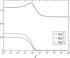
Figure 1: Quark propagator functions (as a function of the momentum squared). The parameters are $\omega=0.5$GeV, $D=16.0$GeV^-2. Left panel: $m_{0}=0$, right panel: $m_{0}=0.115$ GeV. All units are ${\rm GeV}$.

This is the numerical solution to the coupled equations (4), which we emphasize is the basis for the quark solutions for complex momenta. The solution clearly shows that dynamical chiral symmetry breaking is occurring: the mass function $M(p^{2})$ attains a sizable non–zero value, even in the case that the bare quark mass $m_{0}$ is zero. This phenomenon is an example of genuinely non–perturbative behavior as dynamical mass generation cannot occur at any order in perturbation theory. Recall that the effective interaction (1) that enters the Schwinger–Dyson equations does not contain the perturbative UV behavior, rather it has an exponential damping at high momenta. This is manifested in the quark propagator functions as a sharp transition from the low momentum behavior to the bare values in the high momentum region. This transition occurs at about $1{\rm GeV}$.

3 The Bethe-Salpeter Equation

Having obtained the quark propagators in the complex plane from the Schwinger–Dyson equations we have collected all ingredients for the Bethe–Salpeter integral equations. They will ultimately yield the quark meson vertex functions, $\Gamma$, that describe mesons as bound quark–antiquark pairs. These vertex functions for bound states are determined from the condition that the four quark scattering amplitude develops a pole at $P^{2}=-M^{2}$, where $M$ is the mass of the bound state meson.

The vertex functions resulting from the Bethe–Salpeter equation are characterized by three momenta out of which only two are linearly independent due to momentum conservation at the vertex. If we denote the meson momentum $P$ and the momentum of the incoming quark $p+\xi P$ then the momentum of the outgoing quark (= incoming antiquark) is $p+(\xi-1)P$. This suggests to label the vertex functions by $p$ and $P$: $\Gamma(p,P)$. We have introduced the arbitrary momentum partition parameter $\xi\in[0,1]$. Due to strict relativistic covariance the results for physical observables do not depend on $\xi$. We have studied the $\xi$–dependence of our numerical results exhaustively in ref. Alkofer:2002bp . The confirmed $\xi$–independence represents an a posteriori validation for the relativistic covariance of our computations.

We now turn to the main target of our studies, the Bethe–Salpeter integral equations for the vertex function $\Gamma(p,P)$ in ladder approximation alkofer00 ; roberts00 ; tandy :

$$\Gamma(p;P)=-\frac{4}{3}\int\frac{d^{4}k}{(2\pi)^{4}}\,\left[\gamma_{\nu}\,S(k+\xi P)\,\Gamma(k;P)\,S(k+(\xi-1)P)\,\gamma_{\mu}\right]\,g^{2}G_{\mu\nu}(k-p)\,.$$ (5)

Here we have factorized the color factors in the effective interaction, $G_{\mu\nu}^{ab}(q)=\delta^{ab}G_{\mu\nu}(q)$ and performed the corresponding trace. The flavor content of the meson is not made explicit in eq. (5) as we have suppressed the flavor labels in the quark propagators. It is understood that the two propagators in eq. (5) are taken such as to account for the flavor quantum numbers of the considered meson. In the model that we will consider, the up and down quarks will be assumed to have equal current masses ($m_{0}$ in eq. (4)) and thus also identical propagator functions $A(x)$ and $B(x)$. For the light quarks, which should give rise to the familiar $SU(3)_{f}$ nonet, we are thus left with three representatives of each of the multiplets that are distinguished by their isospin number, $I=0,\frac{1}{2},1$ . We must also specify the meson angular momentum and parity. This is reflected by the Dirac and Lorentz decomposition of the meson vertex functions. This decomposition is known in the literature and here we follow ref. llew . For the pseudoscalar channel ($J^{P}=0^{-}$) we take

$$\Gamma^{(P)}(p;P)=\gamma_{5}\left[\Gamma^{(P)}_{0}(p;P)-i\hbox to0.0pt{\hbox to7.80904pt{\hfil/\hfil}\hss}P\Gamma^{(P)}_{1}(p;P)-i\hbox to0.0pt{\hbox to5.03125pt{\hfil/\hfil}\hss}p\Gamma^{(P)}_{2}(p;P)-\left[\hbox to0.0pt{\hbox to7.80904pt{\hfil/\hfil}\hss}P,\hbox to0.0pt{\hbox to5.03125pt{\hfil/\hfil}\hss}p\right]\Gamma^{(P)}_{3}(p;P)\right]\,.$$ (6)

The decomposition for a scalar ($J^{P}=0^{+}$) meson reads

$$\Gamma^{(S)}(p;P)=\Gamma^{(S)}_{0}(p;P)-i\hbox to0.0pt{\hbox to7.80904pt{\hfil/\hfil}\hss}P\Gamma^{(S)}_{1}(p;P)-i\hbox to0.0pt{\hbox to5.03125pt{\hfil/\hfil}\hss}p\Gamma^{(S)}_{2}(p;P)-\left[\hbox to0.0pt{\hbox to7.80904pt{\hfil/\hfil}\hss}P,\hbox to0.0pt{\hbox to5.03125pt{\hfil/\hfil}\hss}p\right]\Gamma^{(S)}_{3}(p;P).$$ (7)

The vector ($J^{P}=1^{-}$) channel involves eight scalar functions

$$\Gamma^{(V)}_{\mu}(p;P) = \left[\gamma_{\mu}-\frac{P_{\mu}\hbox to0.0pt{\hbox to7.80904pt{\hfil/\hfil}\hss}P}{P^{2}}\right]\left[i\Gamma^{(V)}_{0}(p;P)+\hbox to0.0pt{\hbox to7.80904pt{\hfil/\hfil}\hss}P\Gamma^{(V)}_{1}(p;P)-\hbox to0.0pt{\hbox to5.03125pt{\hfil/\hfil}\hss}p\Gamma^{(V)}_{2}(p;P)+i\left[\hbox to0.0pt{\hbox to7.80904pt{\hfil/\hfil}\hss}P,\hbox to0.0pt{\hbox to5.03125pt{\hfil/\hfil}\hss}p\right]\Gamma^{(V)}_{3}(p;P)\right]$$

$$+\left[p_{\mu}-\frac{P_{\mu}p\!\cdot\!P}{P^{2}}\right]\left[\Gamma^{(V)}_{2}(p;P)+2i\hbox to0.0pt{\hbox to7.80904pt{\hfil/\hfil}\hss}P\Gamma^{(V)}_{3}(p;P)\right]$$

$$+\left[p_{\mu}-\frac{P_{\mu}p\!\cdot\!P}{P^{2}}\right]\left[\Gamma^{(V)}_{4}(p;P)+i\hbox to0.0pt{\hbox to7.80904pt{\hfil/\hfil}\hss}P\Gamma^{(V)}_{5}(p;P)-i\hbox to0.0pt{\hbox to5.03125pt{\hfil/\hfil}\hss}p\Gamma^{(V)}_{6}(p;P)+\left[\hbox to0.0pt{\hbox to7.80904pt{\hfil/\hfil}\hss}P,\hbox to0.0pt{\hbox to5.03125pt{\hfil/\hfil}\hss}p\right]\Gamma^{(V)}_{7}(p;P)\right]\,.$$

In the axialvector channel we have two modes that are distinguished by their charge conjugation properties llew . For $J^{PC}=1^{++}$ the decomposition is

$$\Gamma^{(A)}_{\mu}(p;P) = \gamma_{5}\left[\gamma_{\mu}-\frac{P_{\mu}\hbox to0.0pt{\hbox to7.80904pt{\hfil/\hfil}\hss}P}{P^{2}}\right]\left[i\Gamma^{(A)}_{0}(p;P)+\hbox to0.0pt{\hbox to7.80904pt{\hfil/\hfil}\hss}P\Gamma^{(A)}_{1}(p;P)-\hbox to0.0pt{\hbox to5.03125pt{\hfil/\hfil}\hss}p\Gamma^{(A)}_{2}(p;P)+i\left[\hbox to0.0pt{\hbox to7.80904pt{\hfil/\hfil}\hss}P,\hbox to0.0pt{\hbox to5.03125pt{\hfil/\hfil}\hss}p\right]\Gamma^{(A)}_{3}(p;P)\right]$$ (9)

$$+\gamma_{5}\left[p_{\mu}-\frac{P_{\mu}p\!\cdot\!P}{P^{2}}\right]\left[\Gamma^{(A)}_{2}(p;P)+2i\hbox to0.0pt{\hbox to7.80904pt{\hfil/\hfil}\hss}P\Gamma^{(A)}_{3}(p;P)\right]\,,$$

while the $J^{PC}=1^{+-}$ mode is decomposed as

$$\Gamma^{(\tilde{A})}_{\mu}(p;P) = \gamma_{5}\left[p_{\mu}-\frac{P_{\mu}p\!\cdot\!P}{P^{2}}\right]\left[\Gamma^{(\tilde{A})}_{1}(p;P)+i\hbox to0.0pt{\hbox to7.80904pt{\hfil/\hfil}\hss}P\Gamma^{(\tilde{A})}_{2}(p;P)\right.$$ (10)

$$\hskip 85.35826pt\left.-i\hbox to0.0pt{\hbox to5.03125pt{\hfil/\hfil}\hss}p\Gamma^{(\tilde{A})}_{3}(p;P)+\left[\hbox to0.0pt{\hbox to7.80904pt{\hfil/\hfil}\hss}P,\hbox to0.0pt{\hbox to5.03125pt{\hfil/\hfil}\hss}p\right]\Gamma^{(\tilde{A})}_{4}(p;P)\right].$$

In what follows we will omit the superscripts that label the spin and parity channels because these channels do not mix and there should hence be no confusion.

The solution to the Bethe–Salpeter equation not only yields the meson masses but also the meson quark vertex functions that can be used to compute meson properties. Here we will focus on the pseudoscalar decay constants $f_{\pi}$ and $f_{K}$. In order to calculate these, we first have to normalize the vertex functions $\Gamma(p;P)$. The Bethe–Salpeter equation is a homogeneous equation, and thus needs an additional normalization condition. As mentioned previously, that condition is obtained from demanding the pole in the four–quark Green’s function to be unity. For equal momentum partitioning, (i.e. for $\xi=1/2$ only) it reads tandy

$$2P_{\mu} = 3\int\frac{d^{4}k}{(2\pi)^{4}}\,{\rm Tr}\left\{\overline{\Gamma}(k,-P)\frac{\partial S(k+P/2)}{\partial P_{\mu}}\Gamma(k,P)S(k-P/2)\right.$$ (11)

$$\hskip 85.35826pt\left.+\overline{\Gamma}(k,-P)S(k+P/2)\Gamma(k,P)\frac{\partial S(k-P/2)}{\partial P_{\mu}}\right\}$$

where the trace is over Dirac matrices. The conjugate vertex function $\overline{\Gamma}$ is defined as

$$\overline{\Gamma}(p,-P)=C\Gamma^{T}(-p,-P)C^{-1}\,,$$ (12)

where $C=-\gamma_{2}\gamma_{4}$ is the charge conjugation matrix. The quark propagator derivatives are calculated by differentiating the quark Schwinger–Dyson equations (4) analytically and then numerically integrating the corresponding expressions.

The decay constants are finally obtained from the coupling of the axial current to the quark loop tandy

$$f=\frac{3}{M^{2}}\int\frac{d^{4}k}{(2\pi)^{4}}\,{\rm Tr}\left\{\Gamma(k,-P)S(k+P/2)\gamma_{5}\hbox to0.0pt{\hbox to7.80904pt{\hfil/\hfil}\hss}PS(k-P/2)\right\}\,.$$ (13)

The primary subject of this talk is to extract the bound state masses for the various flavor combinations and angular momentum channels. The corresponding projection results in sets of coupled equations for the $\Gamma_{i}$. After carrying out two of the three angular integrals analytically we are left with functions of the squared momenta $p^{2}$ and $P^{2}$ as well as the angle between $p$ and $P$: $z=p\!\cdot\!P/\sqrt{p^{2}P^{2}}$. The $z$–dependence is analyzed by an expansion in Chebyshev polynomials $T_{k}$

$$\Gamma_{i}(p;P)=\sum_{k}(i)^{k}\Gamma_{i}^{k}(p^{2};P^{2})T_{k}(z)\,.$$ (14)

Since the $T_{k}$ form an orthonormal set, we can project the equations for the Dirac components onto $\Gamma_{i}^{k}(p^{2};P^{2})$. Finally, the $k^{2}$–integral in the Bethe–Salpeter equation (5) is implemented numerically as a matrix equation for the unknown $\Gamma_{i}^{k}(p_{j}^{2};P^{2})$, $p_{j}^{2}$ being the discrete values of the momentum squared. The kernel, $K$ of that matrix parametrically depends on the meson momentum $P^{2}$. We solve that matrix equation as an eigenvalue problem by tuning the meson momentum to $P^{2}=-M^{2}$, such that ${\rm Det}(1-K)=0$. This yields the desired meson mass $M$.

In the discussion of numerical results we note that there are four model parameters, $\omega,D,m_{u}$ and $m_{s}$ that we first have to fit to empirical data. To this end, we initially choose the pseudoscalar meson observables $M_{\pi},M_{K}$ and $f_{\pi}$. Then one parameter remains unconstrained by the pseudoscalar sector alone. However, the condition that the quark propagator function reflects dynamical chiral symmetry breaking, i.e. that $M(p^{2}=0)\approx 0.5{\rm GeV}$ leaves only a small window for the remaining choice. All other masses and decay constants are subsequently model predictions. The resulting model parameter and the predicted kaon decay constant $f_{K}$, that is unexpectedly well reproduced, are shown in Table 1.

$\omega$	$D$	$m_{u}$	$m_{s}$	$M_{\pi}$	$f_{\pi}$	$M_{K}$	$f_{K}$
0.40	45.0	$5\times 10^{-3}$	$0.120$	0.135	0.131	0.496	0.164
0.45	25.0	$5\times 10^{-3}$	$0.120$	0.135	0.131	0.496	0.163
0.50	16.0	$5\times 10^{-3}$	$0.115$	0.137	0.133	0.492	0.164
experiment pdg				0.135	0.131	0.498	0.160

Table 1: Parameter sets used and fit results for the pseudoscalar mesons. $M_{\pi}$, $f_{\pi}$ and $M_{K}$ are used as input, $f_{K}$ is predicted. All units are ${\rm GeV}$.

The subsequently predicted meson masses are shown in Tables 2-5. In all cases we have the inequalities $M_{u\bar{u}}<M_{u\bar{s}}<M_{s\bar{s}}$, where the subscript labels the flavor content. These relations just reflect the quark–antiquark picture that is implicit in the present Bethe–Salpeter approach.

Obviously both the pseudoscalar (table 1) and vector mesons (table 2) can be very well described within our model with the choice $\omega\approx 0.5{\rm GeV}$. Our results agree with a previous analysis of the vector mesons based on an effective interaction which included the perturbative type term maris99 . This shows that such terms do not have a large effect on the meson masses, at least for the pseudoscalar and vector cases. Indeed, in the context of low–energy meson phenomenology we conclude that the logarithmic tail, and its associated renormalization represent an unnecessary obfuscation.

$\omega$	$D$	$m_{u}$	$m_{s}$	$M_{\rho}$	$M_{K^{*}}$	$M_{\phi}$
0.40	45.0	$5\times 10^{-3}$	$0.120$	0.748	0.939	1.072
0.45	25.0	$5\times 10^{-3}$	$0.120$	0.746	0.936	1.070
0.50	16.0	$5\times 10^{-3}$	$0.115$	0.758	0.946	1.078
experiment pdg				0.770	0.892	1.020

Table 2: Results for the vector mesons. All units are ${\rm GeV}$.

The situation for the scalar mesons (table 3) is not quite that clear. To begin with the particle data group pdg does not provide a clear picture in this channel but only quotes a wide range for the mass of the lowest scalar (0.4 – 1.2 GeV). More detailed studies of the pseudoscalar scattering amplitudes revealed that the assignment of the scalar meson nonet is not at all established Syr1 . In particular, these mesons may not be simple quark–antiquark bound states but e.g. might contain sizable admixture of 2quark–2antiquark pairs Ja77 . In that respect we might interpret our results as a quark–antiquark model prediction for scalar mesons. Our results suggest that such a picture is too simple for these mesons. One might also speculate that the adopted ladder approximation could be insufficient.

$\omega$	$D$	$m_{u}$	$m_{s}$	$M_{u\overline{u}}$	$M_{u\overline{s}}$	$M_{s\overline{s}}$
0.40	45.0	$5\times 10^{-3}$	$0.120$	0.700	0.917	1.096
0.45	25.0	$5\times 10^{-3}$	$0.120$	0.675	0.908	1.099
0.50	16.0	$5\times 10^{-3}$	$0.115$	0.645	0.903	1.113

Table 3: Results for the scalar mesons. The subscripts of $M$ denote the flavor content. All units are ${\rm GeV}$.

For the axialvector mesons we have two channels that are distinguished by their charge conjugation properties, cf. tables 4 and 5. The quark–antiquark pairs that are bound to axialvector modes with negative charge conjugation eigenvalue tend to be lighter than those with the positive eigenvalue but otherwise equal quantum numbers. Generally we find that our predictions are lower than the assignments made by the particle data group pdg .

$\omega$	$D$	$m_{u}$	$m_{s}$	$M_{u\overline{u}}$	$M_{u\overline{s}}$	$M_{s\overline{s}}$
0.40	45.0	$5\times 10^{-3}$	$0.120$	0.804	0.994	1.128
0.45	25.0	$5\times 10^{-3}$	$0.120$	0.858	1.047	1.182
0.50	16.0	$5\times 10^{-3}$	$0.115$	0.912	1.098	1.230
experiment pdg				1.230	1.270	1.170 ?

Table 4: Results for the axial-vector ($J^{PC}=1^{+-}$) mesons. The question mark indicates that the PDG did not assign the charge conjugation property of the respective resonance. All units are ${\rm GeV}$.

$\omega$	$D$	$m_{u}$	$m_{s}$	$M_{u\overline{u}}$	$M_{u\overline{s}}$	$M_{s\overline{s}}$
0.40	45.0	$5\times 10^{-3}$	$0.120$	0.917	1.117	1.253
0.45	25.0	$5\times 10^{-3}$	$0.120$	0.918	1.124	1.270
0.50	16.0	$5\times 10^{-3}$	$0.115$	0.927	1.140	1.292
experiment pdg				1.230	1.270	1.282

Table 5: Results for the axial-vector ($J^{PC}=1^{++}$) mesons. All units are ${\rm GeV}$.

We recognize from our results that the model predictions change only slightly within the large range of considered model parameters. This confirms that meson static properties are not too sensitive to the conjectural parameter dependence of the timelike quark propagator functions. Presumably meson properties whose computation involves larger timelike momenta will exhibit a stronger sensitivity.

Already from table 4 we observe that by increasing $\omega$ the predicted mass of the $J^{PC}=1^{+-}$ meson with pion flavor quantum numbers approaches the empirical mass. We therefore further increased $\omega$ according to the rules discussed above. For $\omega\sim 0.8GeV$ we reproduced the empirical value for the mass in that channel. However, this happened at the expense of significantly lowering $f_{K}$ and loosing the proper description of the vector mesons. We recall that the parameter $\omega$ has a physical interpretation as the location of the maximum of the interaction. Thus $\omega=0.8GeV$ seems intuitively too large for low–energy hadron physics and an unsatisfactorily description of the $0^{-}$ and $1^{-}$ mesons comes without surprise.

For non–diagonal flavor structures such as $u\bar{s}$, charge conjugation actually is not a sensible quantum number and the corresponding axial vector mesons $1^{++}$ and $1^{+-}$ may mix. In table 6 we present the results obtained from the full calculation that combines the Dirac decompositions (9) and (10).

$\omega$	$D$	$m_{u}$	$m_{s}$	$M_{u\overline{u}}$	$M_{u\overline{s}}$	$M_{s\overline{s}}$
0.40	45.0	$5\times 10^{-3}$	$0.120$	0.807	0.990	1.131
0.45	25.0	$5\times 10^{-3}$	$0.120$	0.861	1.040	1.185
0.50	16.0	$5\times 10^{-3}$	$0.115$	0.915	1.085	1.233

Table 6: Results for the axial-vector mesons allowing for mixing of the Dirac structures in eqs. (9) and (10). All units are ${\rm GeV}$.

Since our Bethe–Salpeter formalism only yields the lowest mass eigenstate within a given channel, the results presented in table 6 should be compared to those in table 4. The tiny changes for the flavor diagonal mesons are numerical artifacts. Surprisingly the changes for the non–diagonal flavor structure are also only of the order 1%. This suggests only a small mixing between the $1^{++}$ and $1^{+-}$ states with the flavor structure $u\bar{s}$ and the $1^{++}$ and $1^{+-}$ channels represent good approximations to the actual eigenstates.

We can extend our model beyond the light flavors up, down and strange. The only modification is the increase of the current quark mass, $m_{0}$. In Fig. 2 we show how the meson masses increase as the (equal) quark masses are increased into the charm sector $m_{c}=1.125{\rm GeV}$.

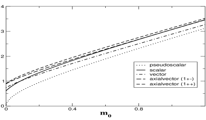
Figure 2: Meson masses as a function of the (equal) quark mass, $m_{0}$. $\omega=0.5GeV,D=16GeV^{-2}$. All units are ${\rm GeV}$.

Exactly the same numerical code is used to construct these solutions to the Schwinger–Dyson and Bethe–Salpeter equations as for the light flavors. Clearly seen is the smooth way the masses increase from the chiral limit ($m_{0}=0$) into the heavy quark sector ($m_{0}=m_{c}$). This represents a convincing indicator for the stability of our technique. The $c\overline{c}$-meson masses can be loosely extracted (table 7) and the data are surprisingly well reproduced.

$J^{P(C)}$	$0^{-}$	$1^{-}$	$0^{+}$	$1^{++}$	$1^{+-}$
$M_{c\overline{c}}$	2.97	3.13	3.32	3.38	3.31
experiment pdg	$\eta_{c}$: 2.98	$J/\psi$: 3.10	$\chi_{c0}$: 3.42	$\chi_{c1}$: 3.51	?

Table 7: Predicted masses of $c\overline{c}$-meson states. $\omega=0.4,D=45.0$, $m_{c}=1.125$. $m_{c}$ is fitted approximately from the $\eta_{c}$ mass.

The lack of the correct UV behavior for the gluon is seemingly at odds with the scales present. However, the present results suggest that the Bethe–Salpeter equation is capable of describing all the angular momentum states equally well in the charm quark sector.

4 Summary and Outlook

In this talk we have presented a study of the low–lying mesons as quark–antiquark bound states in a covariant approach using an effective interaction. This interaction is characterized by gluon exchange with the gluon propagator being dressed by a Gaußian shape function. The interaction is completed by the quark–gluon vertex that we take to be the tree–level perturbative one. In this manner the rainbow–ladder approximation to the system of Schwinger–Dyson and Bethe–Salpeter equation accounts for chiral symmetry. With this effective interaction, we have then consistently treated this system of integral equations by precisely implementing the quark propagator functions that solve the Schwinger–Dyson equations into the Bethe–Salpeter equations. Once the effective interaction exceeds a certain strength, the Schwinger–Dyson equations exhibit dynamical chiral symmetry breaking and the pseudoscalar mesons emerge as would–be Goldstone bosons. We have then used observed properties of the pseudoscalar mesons to determine the model parameters. The kaon decay constant represents a model prediction. It turned out to be in good agreement with the empirical data. Furthermore our results for the vector meson masses match the experimental data. The situation in the scalar channel is less satisfying. As we solely consider the mesons as bound states of quark–antiquark pairs, it is not surprising that the mass eigenvalues increase with the strangeness content. On the other hand it is astonishing that for current quark masses, $m_{0}\geq 0.2{\rm GeV}$, the lightest scalar mesons turn out to be heavier than the lightest vector mesons. When discussing these results it must be noted that the role and structure of the scalar mesons is still under intense debate. In particular, the question whether they should indeed be considered as quark–antiquark bound states is not yet completely resolved. There are indications, see e.g. ref. Syr1 and references therein, that the scalar meson masses should actually decrease with the strangeness content of these mesons. This can be understood if these mesons are considered as 2quark–2antiquark bound states in the sense of diquark–antidiquark systems Ja77 .

As an outlook we mention that there is an elegant way to extend the present model to incorporate such degrees of freedom. The Bethe–Salpeter treatment can be straightforwardly extended to study bound states of diquark–antidiquark pairs, once a binding mechanism is established. This could either be achieved by a gluon exchange similar to eq. (1) or by quark exchange between a quark and a diquark. The latter approach has been intensively studied and the corresponding vertex is known from modeling baryon properties tuediq . It will also be interesting to see whether these additional degrees of freedom will also affect the mass predictions for the axialvector mesons that currently tend to be on the low side. Investigations in this direction are in progress.

References

- (1) D. Black et al., Phys. Rev. D64 (2001) 014031; N. A. Törnquist, hep-ph/0201171; M. Ishida, hep-ph/9905259; N. N. Achasov, hep-ph/0201299.
- (2) J. E. Mandula, Phys.Rept. 315 (1999) 273; F. D. Bonnet, P. O. Bowman, D. B. Leinweber and A. G. Williams, Phys. Rev. D62 (2000) 051501; F. D. Bonnet, P. O. Bowman, D. B. Leinweber, A. G. Williams and J. M. Zanotti, Phys. Rev. D64, (2001) 034501; K. Langfeld, H. Reinhardt and J. Gattnar, Nucl. Phys. B621 (2002) 131.
- (3) R. Alkofer and L. von Smekal, Phys. Rept. 353 (2001) 281.
- (4) L. von Smekal, R. Alkofer and A. Hauck, Phys. Rev. Lett. 79 (1997) 3591; Ann. Phys. 267 (1998) 1.
- (5) C. S. Fischer and R. Alkofer, Phys. Rev. D 67 (2003) 094020 [arXiv:hep-ph/0301094].
- (6) C. D. Roberts and S. M. Schmidt, Prog. Part. Nucl. Phys. 45 (2000) S1.
- (7) Y. Nambu and G. Jona-Lasinio, Phys. Rev. 122 (1961) 345; 124 (1961) 246.
- (8) D. Ebert and H. Reinhardt, Nucl. Phys. B271 (1986) 188.
- (9) P. Jain and H. J. Munczek, Phys. Rev. D48 (1993) 5403; G. Krein, C. D. Roberts and A. G. Williams, Int. J. Mod. Phys. A 7 (1992) 5607.
- (10) P. Maris, C. D. Roberts and P. C. Tandy, Phys. Lett. B420 (1998) 267.
- (11) P. Maris, and P. C. Tandy, Phys. Rev. C60 (1999) 055214.
- (12) C. D. Roberts, Nucl. Phys. A605 (1996) 475.
- (13) P. Maris and C. D. Roberts, Phys. Rev. C56 (1997) 3369.
- (14) A. Bender, C. D. Roberts and L. von Smekal, Phys. Lett. B380 (1996) 7; G. Hellstern, R. Alkofer and H. Reinhardt, Nucl. Phys. A625 (1997) 697; A. Bender et al. Phys. Rev. C 65 (2002) 065203
- (15) R. Alkofer, P. Watson and H. Weigel, Phys. Rev. D65 (2002) 094026.
- (16) R. L. Jaffe, Phys. Rev. D15 (1977) 267.
- (17) P.C. Tandy, Prog. Part. Nucl. Phys 39 (1997) 117.
- (18) C.H. Llewellyn-Smith, Ann. Phys 53 (1953) 521.
- (19) D. E. Groom et al. (Particle Data Group), Eur. Phys. J. C15, (2000) 1, and 2001 partial update for edition 2002 (URL: http://pdg.lbl.gov).
- (20) M. Oettel, G. Hellstern, R. Alkofer and H. Reinhardt, Phys. Rev. C58 (1998) 2459; M. Oettel, M. Pichowsky and L. von Smekal, Eur. Phys. J. A8 (2000) 251; M. Oettel, R. Alkofer and L. von Smekal, Eur. Phys. J. A8 (2000) 553; S. Ahlig et al., Phys. Rev. D64 (2001) 014004; M. Oettel and R. Alkofer, Eur. Phys. J. A 16 (2003) 95