On $\gamma\gamma^{*}$ production of two $\rho^{0}$ mesons

Abstract

We present a theoretical estimation for the cross-section of exclusive two $\rho$-meson production in two photon collision when one of the initial photons is highly virtual. The compatibility of our analysis with recent experimental data obtained by the L3 Collaboration at LEP is discussed. We show that these data prove the scaling behaviour of the exclusive production amplitude. They are thus consistent with a partonic description of the exclusive process $\gamma\gamma^{*}\to\rho^{0}\rho^{0}$ when $Q^{2}\sim 2-20\,{\rm GeV^{2}}$.

I Introduction

Two-photon collisions provide a tool to study a variety of fundamental aspects of QCD and have long been a subject of great interest (cf., e.g., Terazawa ; Bud ; photon-conf and references therein). A peculiar facet of this interesting domain is exclusive two hadron production in the region where one initial photon is highly virtual (its virtuality being denoted as $Q^{2}$) but the overall energy (or invariant mass of the two hadrons) is small DGPT . This process factorizes MRG ; Freund into a perturbatively calculable, short-distance dominated scattering $\gamma^{*}\gamma\to q\bar{q}$ or $\gamma^{*}\gamma\to gg$, and non-perturbative matrix elements measuring the transitions $q\bar{q}\to AB$ and $gg\to AB$. These matrix elements have been called generalized distribution amplitudes (GDAs) to emphasize their close connection to the distribution amplitudes introduced many years ago in the QCD description of exclusive hard processes LepageBrodsky .

In this paper, we focus on the process $\gamma^{*}\gamma\to\rho^{0}\rho^{0}$ which has not been much discussed theoretically (see however Ref. Maul ) but has recently been observed at LEP in the right kinematical domain L3Coll .

Since $\gamma^{*}\gamma\to\rho\rho$ is the crossed channel of virtual Compton scattering on a spin-$1$ meson, the physics considered here is closely related to deeply virtual Compton scattering (DVCS) on a spin-$1$ target CP , which has recently attracted some attention in the context of generalized (skewed) parton distributions of the deuteron BCDP .

II Kinematics

The reaction which we study here is (see, Fig. 1):

$$e(k)+e(l)\to e(k^{\prime})+e(l^{\prime})+\rho^{0}(p_{1})+\rho^{0}(p_{2})$$ (1)

where the initial electron $e(k)$ radiates a hard virtual photon with momentum $q=k-k^{\prime}$, in other words, the square of virtual photon momentum $q^{2}=-Q^{2}$ is very large. This means that the scattered electron $e(k^{\prime})$ is tagged. To describe reaction (1), it is useful to consider, at the same time, the sub-process :

$$e(k)+\gamma(q^{\prime})\to e(k^{\prime})+\rho^{0}(p_{1})+\rho^{0}(p_{2}).$$ (2)

Regarding the other photon momentum $q^{\prime}=l-l^{\prime}$, we assume that, firstly, its momentum is collinear to the electron momentum $l$ and, secondly, that $q^{\prime\,2}$ is approximately equal to zero, which is a usual approximation when the second lepton is untagged.

Let us now pass to a short discussion of kinematics in the $\gamma\gamma^{*}$ center of mass system. We adopt the $z$ axis directed along the three-dimensional vector ${\bf q}$, and the $\rho$-meson momenta lie in the $(x,z)$-plane. It means that we ignore the azimuthal dependence of the cross-section, which happens to be absent in the approximation we use. So, we write for the momenta in the c.m. system :

$$q=(q_{0},\,0,\,0,\,{\bf q}),\quad p_{1}=(p_{1}^{0},\,{\bf p}_{1}{\rm sin}\theta,\,0,\,{\bf p}_{1}{\rm cos}\theta).$$ (3)

Also, we need to write down the Mandelstam $S$-variables for the electron-positron (1) and electron-photon (2) collisions:

$$S_{ee}=(k+l)^{2},\quad S_{e\gamma}=(k+q^{\prime})^{2}.$$ (4)

Neglecting the lepton masses, these variables can be rewritten as

$$S_{ee}\approx 2(k\cdot l),\quad S_{e\gamma}\approx 2(k\cdot q^{\prime})=x_{2}S_{ee},$$ (5)

where the fraction $x_{2}$ defined as $q_{0}^{\prime}=x_{2}l_{0}$ is introduced (see, Diehl00 ).

Figure 1: Kinematics of the process $e(k)+e(l)\to e(k^{\prime})+e(l^{\prime})+\rho^{0}(p_{1})+\rho^{0}(p_{2})$ in the c.m.s of the two mesons.

III Parameterization of $\rho$-matrix elements and their properties

Let us first introduce the basis light-cone vectors. We adopt a basis consisting of two light-like vectors $p$ and $n$ of mass dimension $1$ and $-1$, respectively. In other words, they obey the following conditions :

$$p^{2}=n^{2}=0,\quad(p\cdot n)=1.$$ (6)

With the help of this basis, the $\rho$-mesons momenta $p_{1}$ and $p_{2}$ can be written as

$$p_{1}^{\mu}=\zeta p^{\mu}+(1-\zeta)\frac{W^{2}}{2}n^{\mu}-\frac{\Delta_{T}^{\mu}}{2},$$

$$p_{2}^{\mu}=(1-\zeta)p^{\mu}+\zeta\frac{W^{2}}{2}n^{\mu}+\frac{\Delta_{T}^{\mu}}{2}$$ (7)

As usually for the two meson generalized distribution amplitude case, we introduce the sum and difference of hadronic momenta which take the form in the light-cone decomposition :

$$\Delta^{\mu}=p_{2}^{\mu}-p_{1}^{\mu},\quad P^{\mu}=p_{2}^{\mu}+p_{1}^{\mu}.$$ (8)

The skewedness parameter $\zeta$ is defined by

$$\zeta=\frac{p_{1}^{+}}{P^{+}}=\frac{1+\beta\cos{\theta}}{2},\quad\beta=\sqrt{1-\frac{4m_{\rho}^{2}}{W^{2}}}.$$ (9)

Note also that within the c.m. frame the transverse component of the transfer momentum $\Delta_{T}=(0,{\bf\Delta}_{T},0)$ is given by

$$\Delta_{T}^{2}=-{\bf\Delta}_{T}^{2}=\biggl{(}4m_{\rho}^{2}-W^{2}\biggr{)}\sin^{2}{\theta}.$$ (10)

Let us now write down the decomposition for the longitudinal and transverse $\rho$-meson polarization vectors:

$$e_{1\,\mu}^{(0)}=\frac{1}{m_{\rho}}\biggl{(}p_{1\,\mu}-\frac{m^{2}_{\rho}}{\zeta}n_{\mu}\biggr{)},$$

$$e_{1\,\mu}^{(1)}=\frac{2}{\sqrt{{\bf\Delta}_{T}^{2}}}\Biggl{(}\zeta p_{2\,\mu}-(1-\zeta)p_{1\,\mu}-\frac{\zeta(2\zeta-1)W^{2}+{\bf\Delta}_{T}^{2}}{2\zeta}n_{\mu}\Biggr{)},$$

$$e_{1\,\mu}^{(2)}=-\frac{2}{\sqrt{{\bf\Delta}_{T}^{2}}}\varepsilon_{\mu\alpha\beta\gamma}p_{2\,\alpha}p_{1\,\beta}n_{\gamma},$$ (11)

for the $\rho$-meson with momentum $p_{1}$, and

$$e_{2\,\mu}^{(0)}=\frac{1}{m_{\rho}}\biggl{(}p_{2\,\mu}-\frac{m^{2}_{\rho}}{1-\zeta}n_{\mu}\biggr{)},$$

$$e_{2\,\mu}^{(1)}=-\frac{2}{\sqrt{{\bf\Delta}_{T}^{2}}}\Biggl{(}(1-\zeta)p_{1\,\mu}-\zeta p_{2\,\mu}+\frac{(1-\zeta)(2\zeta-1)W^{2}-{\bf\Delta}_{T}^{2}}{2(1-\zeta)}n_{\mu}\Biggr{)},$$

$$e_{2\,\mu}^{(2)}=\frac{2}{\sqrt{{\bf\Delta}_{T}^{2}}}\varepsilon_{\mu\alpha\beta\gamma}p_{2\,\alpha}p_{1\,\beta}n_{\gamma},$$ (12)

for the other $\rho$-meson with momentum $p_{2}$. As usual,

$$e_{i}\cdot p_{i}=0,\quad e_{i}^{(\lambda)}\cdot e_{i}^{(\lambda^{\prime})}=-\delta^{\lambda\lambda^{\prime}}.$$ (13)

Besides, for each meson, the following polarization vectors can be introduced to define the light-cone helicity :

$$e(0)=e^{(0)},\quad e(\pm)=\frac{\mp e^{(1)}-ie^{(2)}}{\sqrt{2}}.$$ (14)

We now come to the parameterization of the relevant matrix elements. Keeping the terms of leading twist $2$, the vector and axial correlators can be written as:

$$\langle p_{1},\lambda_{1};p_{2},\lambda_{2}|\bar{\psi}(0)\gamma_{\mu}\psi(\lambda n)|0\rangle\stackrel{{\scriptstyle{\cal F}}}{{=}}p_{\mu}\sum_{i}\,e_{1}^{\alpha}e_{2}^{\beta}V^{(i)}_{\alpha\beta}(p_{1},p_{2},n)H^{\rho\rho,\,V}_{i}(y,\zeta,W^{2}),$$ (15)

$$\langle p_{1},\lambda_{1};p_{2},\lambda_{2}|\bar{\psi}(0)\gamma_{\mu}\gamma_{5}\psi(\lambda n)|0\rangle\stackrel{{\scriptstyle{\cal F}}}{{=}}p_{\mu}\sum_{i}\,e_{1}^{\alpha}e_{2}^{\beta}A^{(i)}_{\alpha\beta}(p_{1},p_{2},n)H^{\rho\rho,\,A}_{i}(y,\zeta,W^{2}).$$ (16)

Here $\lambda_{1}$ and $\lambda_{2}$ are the helicities of $\rho$ mesons and $\stackrel{{\scriptstyle{\cal F}}}{{=}}$ denotes the Fourier transformation with measure ($z_{1}=\lambda n,z_{2}=0$) Ani :

$$d\mu(y)=dy\,e^{-iy\,pz_{1}+i(1-y)\,pz_{2}}.$$ (17)

With the help of parity invariance we can show that the vector tensors $V^{(i)}_{\alpha\beta}$ may be written in terms of five tensor structures while the axial tensors $A^{(i)}_{\alpha\beta}$ are linear combinations of four independent structures. In complete analogy with the analysis of the deuteron generalized parton distributions BCDP we write

$$\sum_{i}e_{1}^{\alpha}e_{2}^{\beta}V^{(i)}_{\alpha\beta}(p_{1},p_{2},n)H^{\rho\rho,\,V}_{i}(y)=-(e_{1}\cdot e_{2})\,H^{\rho\rho,\,V}_{1}(y)+$$

$$\biggl{(}(e_{1}\cdot n)(e_{2}\cdot p_{1})+(e_{2}\cdot n)(e_{1}\cdot p_{2})\biggr{)}\,H^{\rho\rho,\,V}_{2}(y)-\frac{(e_{1}\cdot p_{2})(e_{2}\cdot p_{1})}{2m^{2}_{\rho}}\,H^{\rho\rho,\,V}_{3}(y)+$$

$$\biggl{(}(e_{1}\cdot n)(e_{2}\cdot p_{1})-(e_{2}\cdot n)(e_{1}.p_{2})\biggr{)}\,H^{\rho\rho,\,V}_{4}(y)+\biggl{(}4m_{\rho}^{2}\,(e_{1}\cdot n)(e_{2}\cdot n)+\frac{1}{3}(e_{1}\cdot e_{2})\biggr{)}H^{\rho\rho,\,V}_{5}(y)$$ (18)

for the vector tensor structures and

$$\sum_{i}e_{1}^{\alpha}e_{2}^{\beta}A^{(i)}_{\alpha\beta}(p_{1},p_{2},n)H^{\rho\rho,\,A}_{i}(y)=-i\epsilon_{\alpha\beta}^{T}e^{T}_{1\,\alpha}e^{T}_{2\,\beta}\,H^{\rho\rho,\,A}_{1}(y)+$$

$$i\epsilon_{\alpha\beta}^{T}\Delta_{\alpha}\,\frac{e_{1\,\beta}(e_{2}\cdot p_{1})+e_{2\,\beta}(e_{1}\cdot p_{2})}{m_{\rho}^{2}}H^{\rho\rho,\,A}_{2}(y)+i\epsilon_{\alpha\beta}^{T}\Delta_{\alpha}\,\frac{e_{1\,\beta}(e_{2}\cdot p_{1})-e_{2\,\beta}(e_{1}\cdot p_{2})}{m_{\rho}^{2}}H^{\rho\rho,\,A}_{3}(y)+$$

$$i\epsilon_{\alpha\beta}^{T}\Delta_{\alpha}\,\biggl{(}e_{1\,\beta}(e_{2}\cdot n)+e_{2\,\beta}(e_{1}\cdot n)\biggr{)}\,H^{\rho\rho,\,A}_{4}(y)$$ (19)

for the axial tensor structures. In (III) and (III), the standard notation $\epsilon^{T}_{\alpha\beta}=\epsilon_{\alpha\beta\gamma\delta}\,p_{\gamma}n_{\delta}$ was used and the dependence of parameterizing functions (GDA) on $\zeta$ and $W^{2}$ is implied.

Let us now turn to the consideration of symmetry properties. The $\gamma\gamma^{*}$ subprocess is selecting the parts with the following symmetry:

$$H^{\rho\rho,\,V}_{i}(y)=-H^{\rho\rho,\,V}_{i}(1-y),\quad H^{\rho\rho,\,A}_{i}(y)=H^{\rho\rho,\,A}_{i}(1-y)$$ (20)

Note that the scale dependence of generalized distribution amplitudes acquired in the process of factorization of the scattering amplitude has been studied in Diehl00 and there are no essential differences between the $\pi\pi$ channel discussed there and vector contributions to our $\rho\rho$ case. At the same time, the evolution of axial contributions are similar to the case of the distribution amplitudes of singlet axial mesons. The $W^{2}$ behaviour of $2\pi$ GDA’s has been recently explored in terms of an impact representation of the hadronization process $q\bar{q}\to MM$ PS .

IV Quark-hadron helicity amplitudes

Although the main objects of our investigation are the generalized distribution amplitudes (GDA) let us begin from the discussion of the helicity amplitudes related to the generalized parton distribution (GPD), which are related to GDAs by means of $s\leftrightarrow t$ crossing symmetry Pol ; Radon . One considers the quark helicity conserving distributions parameterizing the combination of the vector and axial matrix elements :

$${\cal A}_{(\lambda_{2}\pm\,\leavevmode\nobreak\ ;\,\lambda_{1}\pm)}=\frac{1}{2}\langle p_{2},\lambda_{2}|\bar{\psi}(0)\gamma^{+}(1\pm\gamma_{5})\psi(z)|p_{1},\lambda_{1}\rangle,$$ (21)

where $\lambda$ and $\mu=\pm$ denote the helicities of initial (final) hadrons and quarks, respectively. The matrix elements in (21) are taken between two $\rho$ mesons. In the forward limit when $p_{1}=p_{2}$ helicity conservation takes place and requires $\lambda_{1}+\mu_{1}=\lambda_{2}+\mu_{2}$. The parity transformation, $\lambda_{i}\to-\lambda_{i}$ etc., invariance leads to nine independent helicity amplitudes (21). At the same time the time reversal transformation, $(\mu_{1},\lambda_{1})\leftrightarrow(\mu_{2},\lambda_{2})$, invariance does not lead to any reduction of the number of independent structures owing to $\zeta$-dependence (see, for instance, BCDP ).

As noted before, the crossing transformation relates the helicity amplitudes referring to the GDAs to the corresponding GPDs helicity amplitudes. Indeed, the crossing transformations imply that the initial hadron is replaced by a final hadron with the opposite momentum : $p_{1}\to-p_{1}$ and, therefore, opposite helicities $\lambda_{1}\to-\lambda_{1}$. Similarly, we implement the crossing replacement for the quark fields. Namely, the final quark with helicity $\mu_{2}$ is replaced by the initial antiquark with helicity $-\mu_{2}$. Thus, the quark helicity non-flip amplitudes in $t$-channel come to the amplitudes in $s$-channel where the initial quark and anti-quark helicities are opposite, and vice versa :

$${\cal A}_{(\lambda_{2}\pm\,;\,\lambda_{1}\pm)}^{(t)}\rightarrow A_{(\lambda_{2}-\lambda_{1}\,;\,\mp\pm)}^{(s)}.$$ (22)

Note that the first two indices labeling the helicity amplitudes in (22) or (21) correspond to the helicities in the final state and the last two indices – to the initial state.

Let us now focus on the amplitudes in $s$-channel. As the helicity and chirality of antiquarks are distinguished by sign (in this paper, we consider the case of massless quarks), the chirality conserving quark-antiquark operator will give the combination of quark and antiquark fields with opposite helicities : $\bar{v}_{+}\gamma^{+}u_{+}\leftrightarrow\bar{v}_{(-)}\gamma^{+}u_{(+)}$, where the bracketed subscripts denote the helicity while the unbracketed ones denote the chirality. Therefore, using (15) and (16), we write, forgetting from now on the $(s)$ subscript,

$$A_{(\lambda_{2}\lambda_{1}\,;\,\pm\mp)}=\frac{1}{2}\langle p_{2},\lambda_{2};p_{1},\lambda_{1}|\bar{\psi}(0)\gamma^{+}(1\pm\gamma_{5})\psi(z)|0\rangle.$$ (23)

Further, a straightforward calculation derives the expressions for the helicity amplitudes (cf., BCDP ) :

$$2A_{(++,+-)} = H_{1}^{\rho\rho,\,V}+BH_{3}^{\rho\rho,\,V}-\frac{1}{3}H_{5}^{\rho\rho,\,V}+H_{1}^{\rho\rho,\,A}+2B\biggl{[}H_{2}^{\rho\rho,\,A}+(2\zeta-1)H_{3}^{\rho\rho,\,A}\biggr{]},$$

$$2A_{(0+,+-)} = \sqrt{\frac{2B\zeta}{1-\zeta}}\Biggl{(}H_{1}^{\rho\rho,\,V}-\zeta\biggl{[}H_{2}^{\rho\rho,\,V}+H_{4}^{\rho\rho,\,V}\biggr{]}+\biggl{[}\frac{(2\zeta-1)W^{2}}{4m^{2}_{\rho}}+2(1-\zeta)\biggr{]}H_{3}^{\rho\rho,\,V}-\Biggr{.}$$

. $$\frac{1}{3}H_{5}^{\rho\rho,\,V}+(1-\zeta)H_{1}^{\rho\rho,\,A}+(1-\zeta)\biggl{[}\frac{(2\zeta-1)W^{2}}{m^{2}_{\rho}}+4(1-\zeta)B\biggr{]}\biggl{[}H_{2}^{\rho\rho,\,A}-H_{3}^{\rho\rho,\,A}\biggr{]}+\Biggr{.}$$

. $$\zeta(1-\zeta)H_{4}^{\rho\rho,\,A}\Biggr{)},$$

$$2A_{(-+,+-)} = -2B\Biggl{(}\frac{1}{2}H_{2}^{\rho\rho,\,V}-(2\zeta-1)H_{2}^{\rho\rho,\,A}-H_{3}^{\rho\rho,\,A}\Biggr{)},$$

$$2A_{(00,+-)} = \biggl{[}\left(\frac{1}{2}-\zeta(1-\zeta)\right)\frac{W^{2}}{m^{2}_{\rho}}-4\left(1-\zeta(1-\zeta)\right)B\biggr{]}\biggl{[}H_{1}^{\rho\rho,\,V}-\frac{1}{3}H_{5}^{\rho\rho,\,V}\biggr{]}-$$ (24)

$$\frac{(2\zeta-1)W^{2}}{2m^{2}_{\rho}}\biggl{[}H_{4}^{\rho\rho,\,V}+(2\zeta-1)H_{2}^{\rho\rho,\,V}\biggr{]}+2B\biggl{[}H_{2}^{\rho\rho,\,V}+(2\zeta-1)H_{4}^{\rho\rho,\,V}\biggr{]}+$$

$$\biggl{[}\frac{(2\zeta-1)^{2}W^{4}}{8m^{4}_{\rho}}-2B\left(\frac{(2\zeta-1)^{2}W^{2}}{2m^{2}_{\rho}}+4\zeta(1-\zeta)B\right)\biggr{]}H_{3}^{\rho\rho,\,V}+4\zeta(1-\zeta)H_{5}^{\rho\rho,\,V}.$$

In (IV) the following notation has been used:

$$B=\frac{{\bf\Delta}_{T}^{2}}{16m^{2}_{\rho}\zeta(1-\zeta)}.$$ (25)

V Amplitude of $\gamma\gamma^{*}\to\rho^{0}\rho^{0}$ subprocess

In this section, we consider the $\gamma(q^{\prime})\gamma^{*}(q)\to\rho^{0}(p_{1})\rho^{0}(p_{2})$ subprocess. Following Ani , the amplitude of this subprocess including the leading twist-$2$ terms can be written as

$$T_{\mu\nu}^{\gamma\gamma^{*}\to\rho^{0}\rho^{0}}=\frac{1}{2}\sum_{q=1}^{n_{f}}e_{q}^{2}\int\limits_{0}^{1}dy\Biggl{[}g_{\mu\nu}^{T}E_{-}(y){\bf V}_{q}(y,\cos{\theta},W^{2})-i\epsilon^{T}_{\mu\nu}E_{+}(y){\bf A}_{q}(y,\cos{\theta},W^{2})\Biggr{]},$$ (26)

where

$$E_{\pm}=\frac{1}{1-y}\pm\frac{1}{y}.$$ (27)

In (26), the scalar and pseudo-scalar functions (${\bf V}$, ${\bf A}$) denote the following contractions

$${\bf V}_{q}(y,\cos{\theta},W^{2})=\sum_{i}e_{1}^{\alpha}e_{2}^{\beta}V^{(i)}_{\alpha\beta}H^{\rho\rho,\,V}_{i,\,q}(y,\zeta(\cos{\theta}),W^{2}),$$

$${\bf A}_{q}(y,\cos{\theta},W^{2})=\sum_{i}e_{1}^{\alpha}e_{2}^{\beta}A^{(i)}_{\alpha\beta}H^{\rho\rho,\,A}_{i,\,q}(y,\zeta(\cos{\theta}),W^{2}).$$

The helicity amplitudes are obtained from the usual amplitudes after multiplying by the photon polarization vectors

$$A_{(i,j)}=\varepsilon^{\,\prime\,(i)}_{\mu}\varepsilon^{(j)}_{\nu}T^{\mu\nu}_{\gamma\gamma^{*}\to\rho^{0}\rho^{0}}.$$ (28)

Here, in the $\gamma\gamma^{*}$ c.m. frame, the photon polarization vectors read

$$\varepsilon^{\,\prime\,(\pm)}_{\mu}=\left(0,\frac{\mp 1}{\sqrt{2}},\frac{+i}{\sqrt{2}},0\right),$$

$$\varepsilon^{\,(\pm)}_{\mu}=\left(0,\frac{\mp 1}{\sqrt{2}},\frac{-i}{\sqrt{2}},0\right),\quad\varepsilon^{\,(0)}_{\mu}=\left(\frac{|q|}{\sqrt{Q^{2}}},0,0,\frac{q_{0}}{\sqrt{Q^{2}}}\right),$$ (29)

for the real and virtual photons, respectively.

VI Differential cross sections

We will now concentrate on the calculation of the differential cross section of (1). The amplitude of this process can be written as

$${\cal A}_{ee\to ee\rho^{0}\rho^{0}}=\sum\limits_{i,j}\biggl{[}\bar{u}(l^{\prime})\gamma^{\mu}u(l)\stackrel{{\scriptstyle*}}{{\varepsilon}}^{\,\prime\,(i)}_{\mu}\biggr{]}\frac{1}{q^{\prime\,2}}A_{(i,j)}^{\gamma\gamma^{*}\to\rho^{0}\rho^{0}}\frac{1}{q^{2}}\biggl{[}\stackrel{{\scriptstyle*}}{{\varepsilon}}^{(j)}_{\nu}\bar{u}(k^{\prime})\gamma^{\nu}u(k)\biggr{]}.$$ (30)

This amplitude depends on the polarization states of the produced $\rho$ mesons. Due to parity invariance there are only three independent sets of helicity (photon) amplitudes which we put to be $A_{(+,+)}$, $A_{(+,-)}$ and $A_{(+,0)}$. Let us focus on the leading twist-$2$ helicity amplitude in the unpolarized electrons case, i.e. the $A_{(+,+)}$ amplitude. In this case, the square of the modulus of the amplitude (30) can be presented in the ”factorized” form :

$$\left|{\cal A}_{ee\to ee\rho^{0}\rho^{0}}\right|^{2}=\left|{\cal A}_{e\gamma\to e\rho^{0}\rho^{0}}\right|^{2}\frac{1}{q^{\prime\,4}}\left|{\cal A}_{e\to e\gamma}\right|^{2}$$ (31)

and the scattering cross section is :

$$d\sigma_{ee\to ee\rho^{0}\rho^{0}}=\frac{1}{2S_{ee}}\frac{d^{3}\,l^{\prime}}{(2\pi)^{3}2l^{\prime}_{0}}\,\frac{d^{3}\,p_{1}}{(2\pi)^{3}2p_{1}^{0}}\,\frac{d^{3}\,p_{2}}{(2\pi)^{3}2p_{2}^{0}}\,\frac{d^{3}\,k^{\prime}}{(2\pi)^{3}2k^{\prime}_{0}}\,$$ (32)

$$\left|{\cal A}_{e\gamma\to e\rho^{0}\rho^{0}}\right|^{2}\frac{1}{q^{\prime\,4}}\left|{\cal A}_{e\to e\gamma}\right|^{2}.$$

¿From now in, we will sum over the polarization states of the $\rho$ mesons. Separating the differential cross section for $e\gamma\to e\rho^{0}\rho^{0}$ subprocess, we are able to rewrite (32) in the form :

$$d\sigma_{ee\to ee\rho^{0}\rho^{0}}=\frac{d^{3}\,l^{\prime}}{(2\pi)^{3}2l^{\prime}_{0}}\,\frac{x_{2}}{q^{\prime\,4}}\left|{\cal A}_{e\to e\gamma}\right|^{2}\,d\sigma_{e\gamma\to e\rho^{0}\rho^{0}},$$ (33)

where

$$d\sigma_{e\gamma\to e\rho^{0}\rho^{0}}=\frac{1}{2S_{e\gamma}}\,\frac{d^{3}\,p_{1}}{(2\pi)^{3}2p_{1}^{0}}\,\frac{d^{3}\,p_{2}}{(2\pi)^{3}2p_{2}^{0}}\,\frac{d^{3}\,k^{\prime}}{(2\pi)^{3}2k^{\prime}_{0}}\,\left|{\cal A}_{e\gamma\to e\rho^{0}\rho^{0}}\right|^{2}.$$ (34)

Using the equivalent photon approximation we find the expression for the corresponding cross section :

$$\frac{d\sigma_{ee\to ee\rho^{0}\rho^{0}}}{dQ^{2}}=\int..\int dW^{2}\,d{\rm cos}\theta\,d\phi\,dx_{2}\frac{\alpha}{\pi}F_{WW}(x_{2})\frac{d\sigma_{e\gamma\to e\rho^{0}\rho^{0}}}{dQ^{2}\,dW^{2}\,d{\rm cos}\theta\,d\phi},$$ (35)

where the Weizsacker-Williams function $F_{WW}$ is defined as usual as :

$$F_{WW}(x_{2})=\frac{1+(1-x_{2})^{2}}{2x_{2}}{\rm ln}\frac{Q^{\prime\,2}(x_{2})}{m_{e}^{2}}-\frac{1-x_{2}}{x_{2}},$$ (36)

and the value $Q^{\prime\,2}$ is defined as

$$Q^{\prime\,2}=-q^{\prime\,2}_{max}=\frac{(1-x_{2})}{4}S_{ee}{\rm sin}^{2}\,\alpha_{max}.$$ (37)

The angle $\alpha_{max}$ in (37) is determined by the acceptance of a lepton in the detector (see, for instance, Diehl00 ) and the value of the c.m. energy of the $ee$ collision $\sqrt{S_{ee}}$ is $91\,{\rm GeV}$ at LEP1 and $195\,{\rm GeV}$ at LEP2.

In (35), the cross section for the subprocess can be calculated directly ; we have

$$\frac{d\sigma_{e\gamma\to e\rho^{0}\rho^{0}}}{dQ^{2}\,dW^{2}\,d{\rm cos}\theta\,d\phi}=\frac{\alpha^{3}}{16\pi}\frac{\beta}{S_{e\gamma}^{2}}\,\frac{1}{Q^{2}}\Biggl{(}1-\frac{2S_{e\gamma}(Q^{2}+W^{2}-S_{e\gamma})}{(Q^{2}+W^{2})^{2}}\Biggr{)}\left|A_{(+,+)}(\cos{\theta},W^{2})\right|^{2}$$ (38)

where

$$\left|A_{(+,+)}(\cos{\theta},W^{2})\right|^{2}=\left(\left|{\bf V}(\cos{\theta},W^{2})\right|^{2}+\left|{\bf A}(\cos{\theta},W^{2})\right|^{2}\right).$$ (39)

In (39), the squared and $\rho$ meson polarizations summed functions $|{\bf V}|^{2}$ and $|{\bf A}|^{2}$ read :

$$|{\bf V}(\cos{\theta},W^{2})|^{2}=\frac{1}{4}P^{\alpha_{1}\alpha_{2}}(p_{1})P^{\beta_{1}\beta_{2}}(p_{2})$$

$$\sum_{i,\,q}e_{q}^{2}V^{(i)}_{\alpha_{1}\beta_{1}}\int dy_{1}E_{-}(y_{1})H^{\rho\rho,\,V}_{i,\,q}(y_{1},\cos{\theta},W^{2})\sum_{j,\,q}e_{q}^{2}V^{(j)}_{\alpha_{2}\beta_{2}}\int dy_{2}E_{-}(y_{2})H^{\rho\rho,\,V}_{j,\,q}(y_{2},\cos{\theta},W^{2})$$ (40)

$$|{\bf A}(\cos{\theta},W^{2})|^{2}=\frac{1}{4}P^{\alpha_{1}\alpha_{2}}(p_{1})P^{\beta_{1}\beta_{2}}(p_{2})$$

$$\sum_{i,\,q}e_{q}^{2}A^{(i)}_{\alpha_{1}\beta_{1}}\int dy_{1}E_{+}(y_{1})H^{\rho\rho,\,A}_{i,\,q}(y_{1},\cos{\theta},W^{2})\sum_{j,\,q}e_{q}^{2}A^{(j)}_{\alpha_{2}\beta_{2}}\int dy_{2}E_{+}(y_{2})H^{\rho\rho,\,A}_{j,\,q}(y_{2},\cos{\theta},W^{2}),$$ (41)

where

$$P_{\alpha\beta}(p)=\sum_{\lambda}e^{(\lambda)}_{\alpha}e^{*\,(\lambda)}_{\beta}=-g_{\alpha\beta}+\frac{p_{\alpha}p_{\beta}}{m^{2}_{\rho}}.$$ (42)

As mentioned before, the expressions (VI) and (VI) do not depend on the azimuth $\phi$.

The helicity squared amplitude when the integration over $\cos{\theta}$ is implemented may be written as

$$F_{(+,+)}(W^{2})=\int\limits_{0}^{1}d{\rm cos}\theta\left|A_{(+,+)}(\cos{\theta},W^{2})\right|^{2},$$ (43)

and the cross section takes the form

$$\frac{d\sigma_{ee\to ee\rho^{0}\rho^{0}}}{dQ^{2}}=\frac{25\alpha^{4}}{36\pi}\int\limits_{0}^{1}dx_{2}F_{WW}(x_{2})\Biggl{(}\frac{1}{x_{2}^{2}S_{ee}^{2}Q^{2}}\int\limits_{W^{2}_{min}}^{W^{2}_{max}}dW^{2}\beta\,F_{(+,+)}(W^{2})-\Biggr{.}$$

. $$\frac{2}{x_{2}S_{ee}Q^{2}}\int\limits_{W^{2}_{min}}^{W^{2}_{max}}dW^{2}\frac{\beta\,F_{(+,+)}(W^{2})}{Q^{2}+W^{2}}+\frac{2}{Q^{2}}\int\limits_{W^{2}_{min}}^{W^{2}_{max}}dW^{2}\frac{\beta\,F_{(+,+)}(W^{2})}{(Q^{2}+W^{2})^{2}}\Biggr{)}.$$ (44)

In (VI), the magnitudes of $W^{2}_{min}$ and $W^{2}_{max}$ are defined by the interval covering most of detected two $\rho^{0}$ events, which in the L3 case at LEP L3Coll is :

$$1.21\,{\rm GeV}^{2}<W^{2}<9.0\,{\rm GeV}^{2}.$$ (45)

Since the $\rho$ meson width is large, the lower limit is a matter of convention, but it can be less than $4m_{\rho}^{2}$. Notice, also, that the integrated function $F_{(+,+)}$ is independent of $Q^{2}$ up to logarithms. Besides, the exact $W^{2}$ dependence of this quantity remains unknown unless some modeling is used. However, the mean value theorem gives the possibility to reduce the three different integrals over $W^{2}$ in (VI) to one integration. Indeed, the mean value theorem reads :

$$\int\limits_{W^{2}_{min}}^{W^{2}_{max}}dW^{2}\frac{\beta\,F_{(+,+)}(W^{2})}{Q^{2}+W^{2}}=\frac{1}{Q^{2}+\langle W_{1}\rangle^{2}}\int\limits_{W^{2}_{min}}^{W^{2}_{max}}dW^{2}\beta\,F_{(+,+)}(W^{2}),$$ (46)

$$\int\limits_{W^{2}_{min}}^{W^{2}_{max}}dW^{2}\frac{\beta\,F_{(+,+)}(W^{2})}{(Q^{2}+W^{2})^{2}}=\frac{1}{(Q^{2}+\langle W_{2}\rangle^{2})^{2}}\int\limits_{W^{2}_{min}}^{W^{2}_{max}}dW^{2}\beta\,F_{(+,+)}(W^{2})$$ (47)

with two phenomenological parameters $\langle W_{1}\rangle$ and $\langle W_{2}\rangle$. Let us now discuss the status of these parameters. In principle, each of these parameters is a function of $Q^{2}$, but owing to the unknown $W^{2}$ dependence of hadronic function $F_{(+,+)}$ the $Q^{2}$ dependences of given parameters stay out of the exact computations. Therefore we will deal with $\langle W_{1}\rangle$ and $\langle W_{2}\rangle$ which will be considered in the sense of average value on the whole interval of $Q^{2}$. Notice also that the values of our parameters have actually the same order of magnitude as $Q^{2}$, therefore we need to keep $\langle W\rangle$-parameters in the prefactors of (46) and (47).

¿From (46) and (47), one can see that it is useful to introduce a third phenomenogical parameter :

$$C_{1}=\int\limits_{W^{2}_{min}}^{W^{2}_{max}}dW^{2}\beta\,F_{(+,+)}(W^{2}).$$ (48)

The normalization of our $2\rho$GDA’s and consequently the value of our $C_{1}$ parameter (see, (61)) is difficult to guess. In the $\pi\pi$ case (see, for instance Diehl00 ), the relation of the second moment of the operator defining the GDA to the energy momentum tensor, allowed to relate the value of the second moment of the GDA to the total energy carried by quarks in the $\pi$ meson, which is known from the study of parton distributions in the meson. This analysis required a modest extrapolation of the meson-pair energy to zero, which was legitimate in the two $\pi$ meson case with small $W$, but is very dangerous in the present two $\rho$ meson case, due to the much larger threshold $W_{min}$. Still, one may expect, that some order of magnitude estimate may be provided by such an extrapolation, as will be confirmed by the numerical results below. Moreover, such an analysis may give indirect access to the parton distributions inside a $\rho$ meson, and, in particular, to the spin and orbital angular momenta carried by quarks.

Finally, the cross section (VI) is expressed through these three phenomenological parameters in the following simple way:

$$\frac{d\sigma_{ee\to ee\rho^{0}\rho^{0}}}{dQ^{2}}=\frac{25\alpha^{4}}{36\pi}\,C_{1}\,\int\limits_{0}^{1}dx_{2}F_{WW}(x_{2})\Biggl{(}\frac{1}{x_{2}^{2}S_{ee}^{2}Q^{2}}+\frac{2}{Q^{2}(Q^{2}+\langle W_{2}\rangle^{2})^{2}}-\frac{2}{x_{2}S_{ee}Q^{2}(Q^{2}+\langle W_{1}\rangle^{2})}\Biggr{)}.$$

In the L3 Collaboration analysis, the value $W$ belongs to the interval (45). Hence we are able to conclude that the phenomenological parameters $\langle W_{1}\rangle$ and $\langle W_{2}\rangle$ may take any values inside this interval.

VII Comparison of $\rho$-mesons and lepton pair productions

In this section we compare the $\rho^{0}\rho^{0}$ production with the production of a lepton pair $\mu^{+}\mu^{-}$ in the same kinematics. The cross section of the process $e\gamma\to e\mu^{+}\mu^{-}$ coming through the $\gamma\gamma^{*}$ subprocess is well-known and has the form :

$$\frac{d\sigma_{e\gamma\to e\mu\mu}^{\gamma\gamma^{*}}}{dQ^{2}}=\frac{\alpha^{3}}{4S_{e\gamma}^{2}\,Q^{2}}\int\limits_{4m_{\mu}^{2}}^{W^{2}_{max}}dW^{2}\Biggl{(}1-\frac{2S_{e\gamma}(Q^{2}+W^{2}-S_{e\gamma})}{(Q^{2}+W^{2})^{2}}\Biggr{)}f^{\mu^{+}\mu^{-}}(W^{2}),$$ (50)

where

$$f^{\mu^{+}\mu^{-}}(W^{2})=8\biggl{(}{\rm ln}\frac{1+\beta^{(\mu)}}{1-\beta^{(\mu)}}-\beta^{(\mu)}\biggr{)},\quad\beta^{(\mu)}=\sqrt{1-\frac{4m_{\mu}^{2}}{W^{2}}}.$$ (51)

In (50), we can also apply the mean value theorem. But now, by virtue of the known form of the muon function (51), the analogues of $\langle W_{i}\rangle$ can be explicitly calculated. So, the mean value theorem for the muon case reads :

$$\int\limits_{4m_{\mu}^{2}}^{W^{2}_{max}}dW^{2}\frac{f^{\mu^{+}\mu^{-}}(W^{2})}{Q^{2}+W^{2}}=\frac{1}{Q^{2}+\langle W_{1,\,(\mu)}\rangle^{2}}\int\limits_{4m_{\mu}^{2}}^{W^{2}_{max}}dW^{2}f^{\mu^{+}\mu^{-}}(W^{2}),$$ (52)

$$\int\limits_{4m_{\mu}^{2}}^{W^{2}_{max}}dW^{2}\frac{f^{\mu^{+}\mu^{-}}(W^{2})}{(Q^{2}+W^{2})^{2}}=\frac{1}{(Q^{2}+\langle W_{2,\,(\mu)}\rangle^{2})^{2}}\int\limits_{4m_{\mu}^{2}}^{W^{2}_{max}}dW^{2}f^{\mu^{+}\mu^{-}}(W^{2}).$$ (53)

Whence, we obtain

$$\langle W_{1,\,(\mu)}\rangle^{2}(Q^{2})=R_{1}(Q^{2})-Q^{2},\quad\biggl{(}Q^{2}+\langle W_{2,\,(\mu)}\rangle^{2}\biggr{)}^{2}=R_{2}(Q^{2}),$$ (54)

where the following notations are introduced :

$$R_{n}(Q^{2})=\frac{{\cal K}}{{\cal L}_{n}(Q^{2})}\quad{\cal K}=\int\limits_{4m_{\mu}^{2}}^{W^{2}_{max}}dW^{2}f^{\mu^{+}\mu^{-}}(W^{2}),\quad{\cal L}_{n}(Q^{2})=\int\limits_{4m_{\mu}^{2}}^{W^{2}_{max}}dW^{2}\frac{f^{\mu^{+}\mu^{-}}(W^{2})}{(Q^{2}+W^{2})^{n}}.$$ (55)

The $Q^{2}$- dependences of $\langle W_{i,\,(\mu)}\rangle^{2}$ are shown on Fig. 2. The solid line correspond to the function $\langle W_{1,\,(\mu)}\rangle^{2}(Q^{2})$ and the dashed one to the function $\langle W_{2,\,(\mu)}\rangle^{2}(Q^{2})$. The weak $Q^{2}$- dependence of $\langle W_{i,\,(\mu)}\rangle^{2}$ justifies the possibility to use the averaged $\langle W_{i,\,(\mu)}\rangle^{2}$ when fitting the data. Besides, a fitting procedure gives us the following representation for these functions :

$$\langle W_{1,\,(\mu)}\rangle^{2}(Q^{2})=3.63-0.015\,Q^{2}+0.47\,{\rm ln}Q^{2},$$

$$\langle W_{2,\,(\mu)}\rangle^{2}(Q^{2})=2.90-0.024\,Q^{2}+0.73\,{\rm ln}Q^{2}.$$

Further, the cross section of two $\rho$ meson production can be written as

$$\frac{d\sigma_{ee\to ee\rho^{0}\rho^{0}}}{dQ^{2}}=\int\limits_{0}^{1}dx_{2}F_{WW}(x_{2})\frac{\alpha^{4}}{4\pi}\frac{C_{1}}{Q^{2}S_{e\gamma}^{2}}{\cal N}(x_{2})\int\limits_{4m_{\mu}^{2}}^{W^{2}_{max}}dW^{2}\Biggl{(}1-\frac{2S_{e\gamma}(Q^{2}+W^{2}-S_{e\gamma})}{(Q^{2}+W^{2})^{2}}\Biggr{)}f^{\mu^{+}\mu^{-}}(W^{2}),$$ (56)

where the function ${\cal N}(x_{2})$ is defined by the ratio ( one reminds here that $S_{e\gamma}$ is proportionnal to the $x_{2}$ fraction, see (5)):

$${\cal N}(x_{2})=\frac{{\cal I}_{1}(x_{2})}{{\cal I}_{2}(x_{2})},$$

$${\cal I}_{1}(x_{2})=\frac{25}{9}\Biggl{(}1-\frac{2S_{e\gamma}}{Q^{2}+\langle W_{1}\rangle^{2}}+\frac{2S_{e\gamma}^{2}}{(Q^{2}+\langle W_{2}\rangle^{2})^{2}}\Biggr{)},$$

$${\cal I}_{2}(x_{2})=\Biggl{(}1-\frac{2S_{e\gamma}}{Q^{2}+\langle W_{1,\,(\mu)}\rangle^{2}}+\frac{2S_{e\gamma}^{2}}{(Q^{2}+\langle W_{2,\,(\mu)}\rangle^{2})^{2}}\Biggr{)}\,{\cal K}.$$ (57)

If one considers the case where $Q^{2}$ is large with respect to the invariant mass squared $W^{2}$, we can omit the terms of $O(1/Q^{2})$ and $O({\rm ln}Q^{2}/Q^{4})$ in (VII) and obtain that ${\cal N}$ becomes independent of $x_{2}$ :

$${\cal N}\approx\frac{25}{9\,{\cal K}}=0.01\,{\rm GeV}^{-2}.$$ (58)

We stress that this value has been obtained providing the value of upper limit $W_{max}^{2}$ is fixed (see, (45)). Actually, the value ${\cal N}$ is a function of $W_{max}^{2}$, owing to the $W_{max}^{2}$-dependence of the integral ${\cal K}$ (see, (55)), and this dependence is pretty strong. For example, enhancing $W_{max}^{2}$ up to $16.0\,{\rm GeV}^{2}$ the value ${\cal N}$ will be halved.

Thus, the cross section of our process is related to the cross section of lepton pair production as

$$\frac{d\sigma_{ee\to ee\rho^{0}\rho^{0}}}{dQ^{2}}\sim 0.01\,\,C_{1}\,\,\frac{d\sigma_{ee\to e\mu\mu}^{\gamma\gamma^{*}}}{dQ^{2}}.$$ (59)

In the next section we will show that $C_{1}$ is close to $1.0\,{\rm GeV}^{2}$. Hence, one can see that the cross section of two $\rho$ meson production is suppressed compared to the cross section of two muon production by a factor which is approximately equal to $100$. Note that a factor of suppression of the same order was present in the case of two $\pi$ mesons production Diehl00 .

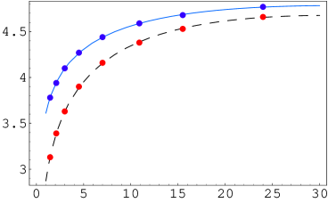
Figure 2: The muonic parameters $\langle W_{1,\,(\mu)}\rangle^{2}$ (solid) and $\langle W_{2,\,(\mu)}\rangle^{2}$ (dashed) as a functions of $Q^{2}$.

VIII Comparision with experimental data

In the previous section we obtained a simple expression for the two mesons cross section as a function of the three parameters $\langle W_{1}\rangle$, $\langle W_{2}\rangle$ and $C_{1}$. Let us now make a fit of these phenomenological parameters in order to get the best description of experimental data. The best values of the parameters can be found by the method of least squares, $\chi^{2}$-method, which flows from the maximum likelihood theorem (see, for instance, Mey ). As usual, the $\chi^{2}$-sum as a function of parameters is written in the form :

$$\chi^{2}=\sum_{i=1}^{N}\Biggl{(}\frac{\sigma^{exp}_{i}-\sigma^{th}_{i}({\bf P})}{\delta\sigma_{i}}\Biggr{)}^{2},$$ (60)

where ${\bf P}=\{\langle W_{1}\rangle,\,\langle W_{2}\rangle,\,C_{1}\}$ denotes the set of fitted parameters ; $\sigma^{exp}_{i}$ and $\sigma^{th}_{i}$ are the experimental measurements of the cross section and its theoretical estimations ; $\delta\sigma_{i}$ are the statistical errors. The experimental data for the cross section of the exclusive double $\rho^{0}$ production were taken from the measurement of the L3 collaboration at LEP L3Coll .

Minimizing $\chi^{2}$-sum in (60) with respect to the parameters ${\bf P}$ we find that the set of solutions ${\bf P}_{min}$ with their confidence intervals are the following :

$$C_{1}=1.20\pm 0.23\,{\rm GeV}^{2},\quad\langle W_{1}\rangle=3.0\pm 1.9\,{\rm GeV},\quad\langle W_{2}\rangle=1.50\pm 0.09\,{\rm GeV}.$$ (61)

With this the magnitude of $\chi^{2}$ is equal to $1.40$ and, therefore, we have

$$\frac{\chi^{2}}{{\rm degree\,of\,freedom}}=0.28<1$$ (62)

The confidence intervals were defined for the case of one-standard deviation. Fig. 3 shows the experimental data with the theoretical fit.

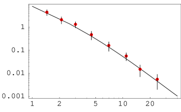
Figure 3: Cross-section $d\sigma_{ee\to ee\rho^{0}\rho^{0}}/dQ^{2}[pb/GeV^{2}]$ as a function of $Q^{2}$ . The theoretical cross-section is plotted for the best fitted parameters which are $C_{1}=1.2\,{\rm GeV}^{2}$ , $\langle W_{1}\rangle=3.0\,{\rm GeV}$ and $\langle W_{2}\rangle=1.5\,{\rm GeV}$.

We can see from (61) that the confidence interval for the parameter $\langle W_{1}\rangle$ covers the whole available interval for $W$.Moreover the obtained values of $\langle W_{2}\rangle$ is quite small. This analysis shows the compatibility of the data with the leading twist analysis which we developed. At the same time, one cannot exclude the existence of sizeable higher twist contributions to the production amplitude. More theoretical and experimental studies are required to make a definite conclusion on higher twist contributions.

IX Conclusion

Data thus are in full agreement with the theoretical expectation on the $Q^{2}$ behaviour of the cross section. Since the effective structure function $F_{(+,+)}$ is expected to be independent of $Q^{2}$ up to logarithms, our analysis of the data is a strong indication of the relevance of the partonic description of the process $\gamma\gamma^{*}\to\rho^{0}\rho^{0}$ in the kinematics of the L3 experiment.

Much more can be done if detailed experimental results are collected. For instance the angular dependence of the final state is a good test of the validity of the asymptotic form of the generalized distribution amplitudes. The spin structure of the final state, if elucidated, would allow to disentangle the roles of the nine generalized distribution amplitudes. The $W^{2}$ behaviour of the cross section may have some interesting features. It depends much on the possible resonances which are able to couple to two $\rho$ mesons. The $\rho^{+}\rho^{-}$ channel may be calculated along the same lines. In that case a brehmstrahlung subprocess where the mesons are radiated from the lepton line must be added. The charge asymmetry then comes from the interference of the two processes. These items will be discussed in a forthcoming publication. More data may be collected at other energies, in particular, in $e^{+}e^{-}$ experiments around $10\,{\rm GeV}$ such as BABAR in SLAC and BELLE in KEK.

X Acknowledgements

We thank I. Boyko, M. Diehl, A. Nesterenko, A. Olchevski and I. Vorobiev for useful discussions and correspondance. This work has been supported in part by RFFI Grant 03-02-16816 and by INTAS Grant (Project 587, call 2000).

References

(1) H. Terazawa, Rev. Mod. Phys. 45, 615
(1973).
(2) V.M. Budnev,
I. F. Ginzburg, G. V. Meledin and V. G. Serbo,
Phys. Rept. 15C, 181
(1975).
(3) S.J. Brodsky, hep-ph/9708345, talk presented at
PHOTON 97, Egmond aan Zee, Netherlands, May 1997;
M.R. Pennington, Nucl. Phys. B (Proc. Suppl.) 82, 291
(2000) [hep-ph/9907353].
(4) M. Diehl, T. Gousset, B. Pire and O.V. Teryaev, Phys. Rev. Lett. 81, 1782 (1998) [hep-ph/9805380];
M. Diehl, T. Gousset and B. Pire, Nucl. Phys. B (Proc. Suppl.) 82, 322 (2000) [hep-ph/9907453].
(5) D. Müller,
D. Robaschik, B. Geyer, F. M. Dittes and J. Horejsi,
Fortschr. Phys. 42, 101 (1994) [hep-ph/9812448].
(6) A. Freund, Phys. Rev. D61, 074010 (2000)
[hep-ph/9903489].
(8)
M. Maul, Phys. Rev. D 63, 036003 (2001)
[arXiv:hep-ph/0003254].
(9)
P. Achard et al. [L3 Collaboration],
Phys. Lett. B 568, 11 (2003)
[arXiv:hep-ex/0305082].
(10)
F. Cano and B. Pire,
Nucl. Phys. A 711 133 (2002) [hep-ph/0211444];
F. Cano and B. Pire,
[hep-ph/0307231];
A. Kirchner and D. Müller,
[hep-ph/0202279];
A. Kirchner and D. Müller,
[hep-ph/0302007].
(11)
E. R. Berger, F. Cano, M. Diehl and B. Pire,
Phys. Rev. Lett. 87 (2001) 142302
[hep-ph/0106192].
(12)
M. Diehl, T. Gousset and B. Pire, Phys. Rev. D 62 (2000) 073014
[hep-ph/0003233].
(13)
B. Pire and L. Szymanowski,
Phys. Lett. B 556, 129 (2003)
[hep-ph/0212296].
(14)
M. V. Polyakov, Nucl. Phys. B 555,231 (1999)
[hep-ph/9809483].
(15)
O. V. Teryaev,
Phys. Lett. B 510, 125 (2001) [hep-ph/0102303].
(16)
I. V. Anikin and O. V. Teryaev,
Phys. Lett. B 509, 95 (2001) [hep-ph/0102209] ;
I. V. Anikin, B. Pire and O. V. Teryaev,
Phys. Rev. D 62, 071501 (2000) [hep-ph/0003203]
(17) S. L. Meyer, ”Data analysis for scientists and
engineers”, Wiley series in probability and mathematical statistics,
Edt. R. A. Bradley and J. S. Hunter, (1975)