Supernova pointing with low- and high-energy neutrino detectors

Abstract

A future galactic SN can be located several hours before the optical explosion through the MeV-neutrino burst, exploiting the directionality of $\nu$-$e$-scattering in a water Cherenkov detector such as Super-Kamiokande. We study the statistical efficiency of different methods for extracting the SN direction and identify a simple approach that is nearly optimal, yet independent of the exact SN neutrino spectra. We use this method to quantify the increase in the pointing accuracy by the addition of gadolinium to water, which tags neutrons from the inverse beta decay background. We also study the dependence of the pointing accuracy on neutrino mixing scenarios and initial spectra. We find that in the “worst case” scenario the pointing accuracy is $8^{\circ}$ at 95% C.L. in the absence of tagging, which improves to $3^{\circ}$ with a tagging efficiency of 95%. At a megaton detector, this accuracy can be as good as $0.6^{\circ}$. A TeV-neutrino burst is also expected to be emitted contemporaneously with the SN optical explosion, which may locate the SN to within a few tenths of a degree at a future km² high-energy neutrino telescope. If the SN is not seen in the electromagnetic spectrum, locating it in the sky through neutrinos is crucial for identifying the Earth matter effects on SN neutrino oscillations.

I Introduction

Observing a galactic supernova (SN) is the holy grail of low-energy neutrino astronomy. The question “how well can one locate the SN in the sky by the neutrinos alone?” is important for two reasons. Firstly, the MeV-neutrino burst precedes the optical explosion by several hours so that an early warning can be issued to the astronomical community Scholberg:1999tm ; snews2 , specifying the direction to look for the explosion. Secondly, in the absence of any SN observation in the electromagnetic spectrum, a reasonably accurate location in the sky is crucial for determining the neutrino Earth-crossing path to various detectors since the Earth matter effects on SN neutrino oscillations may well hold the key to identifying the neutrino mass hierarchy Dighe:1999bi ; Lunardini:2001pb ; Lunardini:2003eh ; Takahashi:2001dc ; Dighe2003 ; Dighe:2003jg .

Nearly contemporaneously with the optical explosion an outburst of TeV neutrinos is expected due to pion production by protons accelerated in the SN shock Waxman2001 . This neutrino burst could produce of order 100 events in a future km² high-energy neutrino telescope, allowing for a pointing accuracy of a few tenths of a degree. Apart from the precise SN pointing, the detection of high-energy neutrinos would be important as the first proof that SN remnants accelerate protons.

The optical signal from a SN, if observed, can give the most accurate determination of its position in the sky. Apart from the observations at the optical telescopes, the multi-GeV to TeV photons associated with the accelerated protons in the shock could be detected on the ground by air Cherenkov telescopes after the SN environment becomes transparent to high-energy photons. If a suitable x- or $\gamma$-ray satellite is in operation at that time, the SN would be visible in these wavebands starting from the optical explosion. A satellite like INTEGRAL could resolve the SN with an angular resolution of 12 arc-minutes integral .

However, it is possible that the SN is not seen in the entire electromagnetic spectrum. This can be the case if it is optically obscured, no suitable x- or $\gamma$-ray satellite operates, and the air Cherenkov telescopes are blinded by daylight or the satellites and telescopes simply do not look in the right direction at the right time. It is also possible that not every stellar collapse produces an explosion so that only neutrinos and perhaps gravity waves can be observed. In such a scenario, the best way to locate a SN by its core-collapse neutrinos is through the directionality of $\nu e^{-}\to\nu e^{-}$ elastic scattering in a water Cherenkov detector such as Super-Kamiokande Beacom:1998fj ; sato . Much less sensitive methods include the time-of-arrival triangulation with several detectors  Beacom:1998fj ; triang or the systematic dislocation of neutrons in scintillation detectors that measure $\bar{\nu}_{e}p\to ne^{+}$ and the subsequent neutron capture Apollonio:1999jg .

The pointing accuracy of Super-Kamiokande or a future megaton detector such as Hyper-Kamiokande or UNO is strongly degraded by the inverse beta reactions $\bar{\nu}_{e}p\to ne^{+}$ that are nearly isotropic and about 30–40 times more frequent than the directional scattering events. Recently it was proposed to add to the water a small amount of gadolinium, an efficient neutron absorber, that would allow one to detect the neutrons and thus to tag the inverse beta reactions vagins . Evidently this would greatly improve the pointing: a tagging efficiency of 90% would double the pointing accuracy vagins . At high tagging efficiency, however, the nearly isotropic oxygen reaction $\nu_{e}+{}^{16}{\rm O}\to{\rm X}+e^{-}$ remains as the dominant background limiting the pointing accuracy. In this paper we analyze the realistic pointing accuracy of a water Cherenkov detector as a function of the neutron tagging efficiency.

The directionality of the elastic scattering reaction is primarily limited by the angular resolution of the detector and to a lesser degree by the kinematical deviation of the final-state positron direction from the initial neutrino. Extracting information from “directional data” is a field in its own right FLE ; Mardia . An efficient method is the “brute force” maximum likelihood estimate of the electron events, taking into account the angular resolution function of the detector on top of a nearly isotropic background. For a large number of events, the accuracy with this method in fact asymptotically approaches the minimum variance as given by the Rao-Cramér bound Rao ; cramer . However, for a small number of signal events, $N_{s}\lesssim 200$, we find that a fraction of the information content of the data as measured by the Fisher information fisher-paper cannot be extracted by even the maximum likelihood method. Using the Rao-Cramér bound therefore overestimates the pointing accuracy of an experiment for small $N_{s}$. In this paper, we determine the realistic accuracy by using a concrete and nearly optimal estimation method.

Since the angular resolution depends on the event energy, the likelihood method requires as input the functional form of the neutrino energy spectra that are only poorly known. It is difficult to systematically take into account the errors introduced by a wrong choice of the fit function for the likelihood method. Therefore we look for “parameter-free” methods like harmonic analysis that use only the information contained in the data and exploit the symmetry of the physical situation. We discuss the efficiency of two methods closely related to the harmonic analysis and find a simple iterative procedure making them nearly as efficient as the maximum likelihood approach. We use the most efficient method thus obtained for analyzing the simulated events at a detector. This makes our estimations realistic and even a bit conservative, since the existence of a better parameter-free method is not excluded. We also study the dependence of the pointing accuracy on the neutrino mixing parameters and the initial neutrino spectra, and use the “worst case” scenario in order to estimate the accuracy.

Finally, we briefly study the pointing accuracy in high-energy neutrino telescopes that can pick up the TeV neutrino burst expected around the time of the optical explosion. While an accurate pointing is easy for any of the existing and future neutrino telescopes if the neutrinos are observed through the Earth, it is far more difficult against the atmospheric muon background from above. Even this would be possible for future km² detectors such as IceCube or Nemo that could detect around $100$ SN events with TeV energies within about one hour.

We begin in Sec. II with a discussion of the statistical methodology for extracting information from directional data using a toy model. In Sec. III we study the realistic SN pointing accuracy of water Cherenkov detectors as a function of the neutron tagging efficiency, using realistic SN neutrino spectra. In Sec. IV we turn to the pointing accuracy of high-energy neutrino telescopes. Sec. V is given over to conclusions.

II Analyzing directional data

II.1 Pointing with maximum likelihood estimate

As a first case we study SN pointing with the $\nu$-$e$ elastic scattering events in the absence of any other background, thus obtaining a bound on the realistic pointing accuracy. To this end we use the toy model introduced in Ref. Beacom:1998fj , i.e. we imagine a directional signal that is distributed as a two-dimensional Gaussian on a sphere. This choice is motivated by the observation that the scatter of signal event directions is dominated by the angular resolution of the detector, and by the assumption that the angular resolution function is Gaussian. Later in Sec. III we consider a more realistic approximation to the angular detector response.

The angular width of the assumed Gaussian distribution is denoted by $\delta_{s}$, where $s$ stands for “signal.” As a further simplification we assume $\delta_{s}\ll\pi/2$, allowing us to approximate the sphere by a plane. Taking the signal to be centered at $\vartheta_{0}=0$, the probability distribution function (pdf) of the signal events is

$$f_{s}(\vartheta,\phi)d\vartheta d\phi=\frac{1}{\cal C}\exp\left(-\frac{\vartheta^{2}}{2\delta_{s}^{2}}\right)d\mu$$ (1)

with $d\mu=\sin\vartheta d\vartheta d\phi$. Here ${\cal C}\equiv\int d\mu\exp[-\vartheta^{2}/(2\delta_{s}^{2})]$ is a normalization constant taking the value ${\cal C}=2\pi\delta_{s}^{2}$ for planar geometry.

In the case of Super-Kamiokande, around 300 elastic scattering events constitute the directional signal. Assuming the mean electron energy to be 11 MeV, a cone with opening angle $\ell_{68}\approx 25^{\circ}$ around the true direction contains 68% of the reconstructed directions Nakahata:1998pz . Solving

$$\int_{0}^{2\pi}d\phi\int_{0}^{(\ell_{68}\pi/180^{\circ})}\!d\vartheta\,f_{s}(\vartheta,\phi)=0.68~{},$$ (2)

we find $\delta_{s}\approx 17^{\circ}$. For $N_{s}~{}\gg~{}1$ signal events without background, the Central Limit Theorem implies that the mean reconstructed direction is within $\delta_{s}/\sqrt{N_{s}}$ of the true direction for 68% of all SN obervations. This quantity, which is $\approx 1^{\circ}$ for 300 events, gives the absolute lower bound on the pointing accuracy in the absence of all backgrounds. We note that Ref. Beacom:1998fj uses $\delta_{s}\approx 25^{\circ}$ and hence obtains $1.5^{\circ}$ for the pointing accuracy. We further note that our $\delta_{s}/\sqrt{N_{s}}\approx 1^{\circ}$ implies that 95% of all SN reconstructions lie within a circle of angular radius $2.4^{\circ}$ of the true direction.

The main degradation of the pointing accuracy is caused by the nearly isotropic inverse beta decay background. The extent of this degradation was addressed for the first time in Ref. Beacom:1998fj . The pdf on a sphere that represents $N_{s}$ signal events distributed like a Gaussian around the direction $(\vartheta_{0},\phi_{0})$ as well as the $N_{b}$ isotropic background events is

$$f(\vartheta,\phi|\vartheta_{0},\phi_{0})\,d\vartheta\,d\phi$$

$$=\,\frac{d\mu}{N_{b}+N_{s}}\left[\frac{N_{b}}{4\pi}+\frac{N_{s}}{{\cal C}}\exp\left(-\frac{\ell^{2}}{2\delta_{s}^{2}}\right)\right]~{},$$ (3)

where

$$\ell\equiv\cos^{-1}[\cos\vartheta\cos\vartheta_{0}+\sin\vartheta\sin\vartheta_{0}\cos(\phi-\phi_{0})]$$ (4)

is the angular distance between the direction of an incoming neutrino and the experimentally measured direction of the Cherenkov cone. We have introduced here the usual notation $f(x|x_{0})$ for the pdf to stress the dependence of $f$ on the data $x=(\phi,\vartheta)$ and the parameters $x_{0}=(\phi_{0},\vartheta_{0})$.

The maximum likelihood estimate (MLE) method is the most efficient way to extract information from statistical data. For the pdf of Eq. (II.1) the likelihood function for $N$ events is

$$L(\vartheta_{0},\phi_{0})\propto\prod_{\alpha=1}^{N}f(\vartheta^{(\alpha)},\phi^{(\alpha)}|\vartheta_{0},\phi_{0})~{},$$ (5)

where $(\vartheta^{(\alpha)},\phi^{(\alpha)})$ are the coordinates of the $\alpha^{\rm th}$ event.

One commonly uses the Fisher information matrix fisher-paper to estimate a lower bound on the uncertainty of the parameters extracted by the MLE method. In our case the Fisher matrix is defined as

$$F_{ij}\equiv\left\langle\frac{\partial^{2}\ln L(\vartheta_{0},\phi_{0})}{\partial\Theta_{i}\partial\Theta_{j}}\right\rangle~{},$$ (6)

where $i,j=1,2$, $\Theta_{1}\equiv\vartheta_{0}$, $\Theta_{2}\equiv\phi_{0}$ and $\langle\ldots\rangle$ denotes an average with respect to $fd\vartheta d\phi$. Since the off-diagonal elements of this matrix vanish, the error in the measurement of the two angles is simply given by

$$\Delta\Theta_{i}=\sqrt{1/F_{ii}}~{}.$$ (7)

This lower bound on the pointing error is also known as the Rao-Cramér bound Rao ; cramer .

For the sake of definiteness, we have chosen the SN direction to lie in the equatorial plane so that $\Delta\vartheta_{0}=\Delta\phi_{0}$, and define the pointing error $\Delta\vartheta$ as

$$\Delta\vartheta\equiv\sqrt{\frac{1}{N-1}\sum{(\bar{\vartheta}-\langle\bar{\vartheta}\rangle)^{2}}}~{},$$ (8)

where $\bar{\vartheta}$ is the estimate for $\vartheta_{0}$ from a given method and $N$ is the number of simulations used. The Rao-Cramér bound corresponds to the inequality

$$(\Delta\vartheta)^{2}\geq(\Delta\vartheta)^{2}_{\rm Fisher}\equiv 1/F~{},$$ (9)

where $F$ may be $F_{11}$ or $F_{22}$.

The accuracy of the MLE method approaches asymptotically the Rao-Cramér bound for a sufficiently large number of events stat-book . For a finite number of data points, the MLE saturates this bound only if the pdf used in the MLE can be written in the product form

$$f(x|x_{0})=g(x_{0})h(x)\exp[A(x_{0})B(x)]~{}.$$ (10)

If the pdf cannot be written in this form, the efficiency of the MLE is significantly smaller than unity at low values of $N_{s}$.

In Fig. 1 we show the efficiency $\varepsilon$ of the MLE in “Fisher units”,

$$\varepsilon\equiv(\Delta\vartheta)^{2}_{\rm Fisher}/(\Delta\vartheta)^{2}~{},$$ (11)

as a function of the number $N_{s}$ of signal events while keeping the background-to-signal ratio $N_{b}/N_{s}$ fixed at 30, which is the expected ratio of the inverse beta decay events to the elastic scattering events in a water Cherenkov detector. Though the MLE efficiency tends asymptotically to the Rao-Cramér bound for large values of $N_{s}$, this bound overestimates the MLE pointing accuracy by $\sim 10$% for $N_{s}\lesssim 200$.

We stress that the Rao-Cramér bound as an estimate of the MLE pointing efficiency is useful only in the limit where the spherical nature of our problem can be approximated by a planar geometry, i.e. when the angular resolution of the detector is much better than $90^{\circ}$. This condition is satisfied in our case. For the general case of a pdf defined on a sphere the MLE still provides an optimal method to determine the pointing accuracy, but the Fisher information matrix no longer provides a direct asymptotic bound on the pointing accuracy. We are not aware of a generalized version of the Rao-Cramér bound that would relate directly to the variance of the pointing estimate in the case of a truly spherical problem.

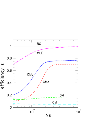
Figure 1: Efficiencies of different estimation methods described in the text for $N_{b}/N_{s}=30$. RC corresponds to the Rao-Cramér minimum variance.

II.2 Efficiencies of parameter-free methods

The MLE is an optimal method to extract information from experimental data if the probability distribution function is known. This is not the case in our situation, where the exact forms of the neutrino spectra are needed and these are only poorly known. It is therefore worthwhile to look for other methods which may be less efficient, but which do not depend on the exact form of the pdf. In our case of SN pointing we wish to consider methods that do not depend on prior knowledge of the exact neutrino energy spectra.

Let us consider two pointing methods that exploit the symmetries of our physical situation, but are independent of the exact details of the pdf. If the efficiency of such a method turns out to be comparable to the maximum likelihood method for the toy model of the previous section, then that method may be expected to be efficient also in the realistic case where the exact pdf is not known and the MLE method cannot be employed.

One obvious approach is the “center of mass” (CM) method. The center of mass $\bf{S}$ of the events,

$$S_{i}\equiv\sum_{\alpha=1}^{N}m^{(\alpha)}x_{i}^{(\alpha)}\,,\qquad i=1,2,3~{},$$ (12)

is taken to be the estimator of the true center of the distribution, where $\bf{x}\equiv(\sin\vartheta\cos\phi,\sin\vartheta\sin\phi,\cos\vartheta)$. For an ideal detector the event weights $m^{(\alpha)}$ are equal and can be set to one. More realistically, the detection probability $p$ is a function of the detection angles $\vartheta,\phi$ and the weight is $m^{(\alpha)}=1/p(\vartheta^{(\alpha)},\phi^{(\alpha)})$.

A second approach is the “orientation matrix” (OM) method FLE . Here, the major principal axis of the orientation matrix

$$T_{ij}\equiv\sum_{\alpha=1}^{N}m^{(\alpha)}x^{(\alpha)}_{i}x^{(\alpha)}_{j}$$ (13)

is taken to be the estimator.

These two methods are equivalent to a harmonic analysis,

$$a_{lm}=\sum_{\alpha=1}^{N}Y_{lm}(\vartheta^{(\alpha)},\phi^{(\alpha)})~{},$$ (14)

restricted to the first moment for CM, and up to the second moment for OM. This equivalence can be seen either by a direct evaluation of Eq. (14) or by identifying $S_{i}$ with a dipole moment and relating $T_{ij}$ to a quadrupole moment $Q_{ij}$. Since $3T_{ij}=Q_{ij}+N\delta_{ij}$, the direction of the major principal axis is identical for both ellipsoids. Note that the orientation matrix is a reducible tensor and therefore contains information from the first as well as the second moment.

Neither of these methods requires any prior knowledge of the neutrino spectra or cross sections. However, they involve some loss of information and hence will give larger pointing errors than the MLE. In order to quantify the efficiency of these methods we generate a data sample according to the pdf of Eq. (3) and show the respective pointing errors in Fig. 2. We keep the number of signal events fixed at $N_{s}=300$, and show the pointing error $\Delta\vartheta$ as a function of $N_{b}/N_{s}$. Note that in the absence of neutron tagging this ratio is expected to be around 30–40.

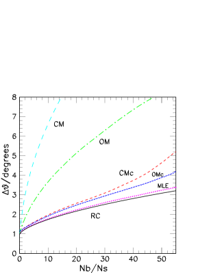
Figure 2: Pointing error $\Delta\vartheta$ for different estimation methods for $N_{s}=300$. RC corresponds to the minimum variance as given by the Rao-Cramér bound.

Figure 2 shows that the error of MLE is almost the same as the Rao-Cramér (RC) bound. However, the errors of CM and OM are much larger. One may also notice that OM is more accurate than CM. This difference may be attributed to the fact that whereas CM tries to exploit the spherical symmetry of the background, OM exploits the cylindrical symmetry of the background about the arrival direction, which is broken much more weakly by statistical fluctuations in the background. Moreover, in terms of a harmonic analysis, OM involves information from both $l=1$ and 2 while CM involves only $l=1$.

In order to increase the efficiency of CM and OM, we use the physical input that the signal is concentrated within a small region around the peak. Cutting off the events beyond a certain angular radius would then increase the signal to background ratio and the above methods may be applied iteratively to this new data. This procedure converges quickly and gives a much better estimate of the incoming neutrino direction. The optimal value of the angular cut has a very weak dependence on the number of events and the background-to-signal ratio. It depends mainly on the value of $\delta_{s}$ and is found to lie between $2\delta_{s}$ and $3\delta_{s}$. Within this range, the efficiency depends only weakly on the exact value of the angular cut. We tried both a sharp cutoff and a Gaussian weight function; both choices give practically identical results.

The optimal value of the cut also increases slowly with decreasing background-to-signal ratio, and in the limit of zero background, the method without cut is clearly more efficient than the method with cut since the latter now cuts off signal but no background. However, the variation due to changing the cut is of the order of only a few percent. Therefore, we keep the value of the cut to be constant at $40^{\circ}$ for the analysis in this section. Our results for the pointing accuracy will therefore be somewhat conservative.

We denote the CM and OM methods with this cutting procedure by CMc and OMc, respectively. Figure 2 shows how the pointing error decreases drastically with the cutting procedure. It may also be observed that the accuracy of CMc stays close to that of MLE for low values of the background-to-signal ratio, while the accuracy of OMc is close to MLE in the entire $N_{b}/N_{s}$ range.

The efficiencies of all methods depend on both $N_{s}$ and $N_{b}/N_{s}$. In Fig. 1 we show the efficiency $\varepsilon$ for different methods as a function of $N_{s}$, keeping $N_{b}/N_{s}$ fixed at 30. For a large number of signal events, $N_{s}\gtrsim 300$, all methods tend to their asymptotic efficiencies $\varepsilon_{\infty}$. The OMc method is close to its asymptotic efficiency $\varepsilon_{\infty}\approx 0.77$ already for $N_{s}\approx 200$ whereas CMc needs $N_{s}\approx 300$ events to reach $\varepsilon_{\infty}\approx 0.71$. Since the OMc method turns out to be more efficient that CMc in all the parameter ranges, henceforth we continue using only the OMc method for further estimations.

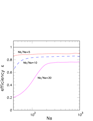
Figure 3: Efficiency of OMc with a $40^{\circ}$ angular cut for different values of $N_{b}/N_{s}$.

With neutron tagging, the value of $N_{b}/N_{s}$ decreases, and that increases the efficiency of the OMc method. In Fig. 3, we show the efficiency of OMc at different values of $N_{b}/N_{s}$. At $N_{b}/N_{s}=10$, which corresponds to the tagging efficiency $\varepsilon_{\rm tag}\approx 67\%$, the asymptotic efficiency of OMc already increases to 0.85, and at $N_{b}/N_{s}=5$, corresponding to $\varepsilon_{\rm tag}\approx 83\%$, it reaches 0.90. Moreover, with decreasing $N_{b}/N_{s}$ the asymptotic value is reached at lower and lower number of signal events. For higher tagging efficiencies, the optimal value of the angular cut increases. In fact, as noted before, in the limit of no background the OM method without the cut is more optimal. However this limit is physically not reached due to the presence of oxygen events.

The OMc method thus sacrifices less than 25%, and at higher tagging efficiency, even less than 15%, of the pointing accuracy of the MLE method. On the other hand, it has the great advantage of being independent of the detailed neutrino spectra and cross sections. Therefore, this method can be extremely useful for a fast analysis of the SN signal. After all, an early warning would depend on a quick and simple data analysis while later one can certainly optimize by fitting detailed energy spectra to the observed signal.

We stress that our preference for a parameter-free method over MLE in this analysis is strongly influenced by the current status of our knowledge regarding the pdf of the angular distribution. It may indeed be possible to use MLE and include all the systematic uncertainties, perhaps giving a better estimate for the pointing accuracy. However, faced with a tradeoff between model independence and higher efficiency, we give more weight to the former. If in future we understand the primary spectra much better than we do now, this preference may change.

III Supernova pointing accuracy of water Cherenkov detectors

We now apply our method to a more realistic representation of the SN signal in a water Cherenkov detector. We shall limit our analysis of the pointing accuracy to our best parameter-free method, i.e. the Orientation Matrix method with an angular cut (OMc).

In order to determine the pointing accuracy numerically we simulate a large ensemble of SN signals in a water Cherenkov detector, assuming different efficiencies for neutron tagging. To this end we assume that the SN is at a distance $D=10$ kpc and releases the neutron-star binding energy $E_{b}=3\times 10^{53}$ erg in the form of neutrinos. Details of the assumed neutrino spectra and fluxes are given in Appendix A. The spread in the predicted neutrino spectra has been taken care of by using two models, a model from the Garching group (model G) garching-model and a model from the Livermore group (model L) livermore-model as described in the same appendix. We take into account the effects of neutrino flavor conversions by considering the three mixing scenarios, (a) normal mass hierarchy and $\sin^{2}\Theta_{13}\gtrsim 10^{-3}$, (b) inverted mass hierarchy and $\sin^{2}\Theta_{13}\gtrsim 10^{-3}$, and (c) any mass hierarchy and $\sin^{2}\Theta_{13}\lesssim 10^{-3}$. The six combinations of the models and neutrino mixing scenarios are represented by G-a, G-b, G-c, L-a, L-b, L-c. We use $\sin^{2}(2\Theta_{\odot})=0.9$ for the solar neutrino mixing angle.

As reaction channels we use elastic scattering on electrons $\nu e^{-}\to\nu e^{-}$, inverse beta decay $\bar{\nu}_{e}p\to ne^{+}$, and the charged-current reaction $\nu_{e}+{}^{16}{\rm O}\to X+e^{-}$, while neglecting the other, subdominant reactions on oxygen. The cross sections for these reactions are summarized in Appendix B. The oxygen reaction is included because it provides the dominant background for the directional electron scattering reaction in a detector configuration with neutron tagging where the inverse beta reaction can be rejected.

For the detector we assume perfect efficiency above an “analysis threshold” of 7 MeV, and a vanishing efficiency below this energy. The actual detector threshold may be as low as 5 MeV. Though lowering the threshold increases the ratio of elastic scattering events and the inverse beta events, it also introduces a background from the neutral-current excitations of oxygen (see Appendix B). In order to avoid additional uncertainties from the cross section of these oxygen reactions, we use the higher analysis threshold. We have checked that the net improvement by lowering the threshold to 5 MeV is less than 10% in all cases.

We assume a fiducial detector mass of 32 kiloton of water. Using the neutrino spectra and mixing parameters from the six cases mentioned above, we obtain 250–300 electron scattering events, 7000–11500 inverse beta decays, and 150–800 oxygen events. The ranges correspond to the variation due to the six different combinations of neutrino mixing scenarios and models for the initial spectra.

The procedure of event generation is described in Appendix C. The angular resolution function of the Super-Kamiokande detector does not follow a Gaussian distribution, rather it is close to a Landau distribution that we use for our simulation. In Fig. 4, the angular distribution of $\bar{\nu}_{e}p\to ne^{+}$ events (green) and elastic scattering events $\nu e^{-}\to\nu e^{-}$ (blue) of one of the simulated SNe are shown in Hammer-Aitoff projection, which is an area preserving map from a sphere to a plane.

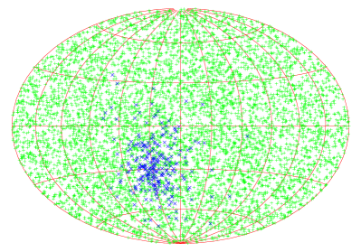
Figure 4: Angular distribution of $\bar{\nu}_{e}p\to ne^{+}$ events (green) and elastic scattering events $\nu e^{-}\to\nu e^{-}$ (blue) of one simulated SN.

The position of the SN is estimated with the OMc method. As explained in Sec. II, the optimal value of the angular cut depends on the neutron tagging efficiency as well as the neutrino spectra. We use a sharp cutoff with $30^{\circ}$ opening angle for the OMc, which may not be optimal, but is observed to be close to optimal in almost the whole parameter range. For low values of $\varepsilon_{\rm tag}$, the value of the cut should be lowered whereas for large values of $\varepsilon_{\rm tag}$ it should be increased by about $10^{\circ}$. The optimal cut depends also on the details of the detector properties and neutrino spectra.

A histogram of the angular distances between the true and the estimated SN position found in $40000$ simulated SNe for different neutron tagging efficiencies for the case G-a is shown in Fig. 5. The histogram fits well the distribution

$$f(\ell)d\ell=\frac{1}{\delta^{2}}\exp\left(-\frac{\ell^{2}}{2\delta^{2}}\right)\ell d\ell~{},$$ (15)

where $\ell$ is the angle between the actual and the estimated SN direction, and $\delta$ is a fit parameter.

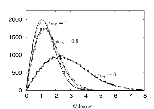
Figure 5: Histogram of the angular distance $\ell$ of the estimated SN direction to the true one for $40000$ simulated SNe with neutrino parameters corresponding to G-a and neutron tagging efficiencies $\varepsilon_{\rm tag}=0,0.8$ and 1. The fits using the distribution in Eq. (15) are also shown.

Defining the opening angle $\ell_{\alpha}$ for a given confidence level $\alpha$ as the value of $\ell$ for which the SN direction estimated by a fraction $\alpha$ of all the experiments is contained within a cone of opening angle $\ell$, we show in Fig. 6 the opening angle for 95% C. L. for the six cases of neutrino parameters. Clearly, the pointing accuracy depends weakly on the neutrino mixing scenario as well as the initial neutrino spectra. Some salient features of this dependence may be understood qualitatively as follows.

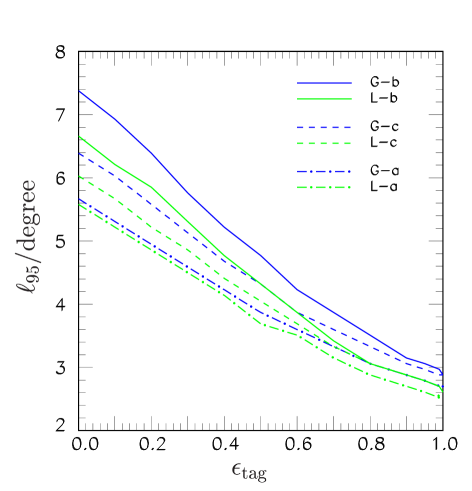
Figure 6: The pointing accuracy $\ell_{95}$ as a function of the neutron tagging efficiency $\varepsilon_{\rm tag}$ for six cases corresponding to three neutrino mixing scenarios and two models for the initial neutrino spectra.

The signal events are dominated by $\nu_{e}$. Indeed, nearly half of the elastic scattering events are due to $\nu_{e}$, whereas the remaining half are due to the other five neutrino species. The cross section of electron scattering events increases with energy. Therefore, the more energetic the $\nu_{e}$ arriving at the detector, the larger the number of signal events and the better the pointing accuracy. Though the initial average $\nu_{e}$ energies are equal in the models G and L, the model L gives a much larger average energy for the initial $\nu_{x}$ spectrum. The $\nu_{e}$-$\nu_{x}$ mixing then tends to give more energetic $\nu_{e}$ in the model L. As a result, for each mixing scenario, the model L predicts a better pointing accuracy than the model G.

Within a model, the pointing accuracy is governed by the background-to-signal ratio. Since the cross section of the dominating background $\bar{\nu}_{e}p$ reaction increases with energy, more $\bar{\nu}_{e}$-$\nu_{x}$ mixing tends to give more energetic $\bar{\nu}_{e}$ and hence more background and less pointing accuracy. The ratio of $\bar{\nu}_{e}$-$\nu_{x}$ mixing to $\nu_{e}$-$\nu_{x}$ mixing within a model is the smallest for the mixing scenario (a) and the largest for the scenario (b). Therefore, within a model the scenario (a) always gives the best pointing accuracy and the scenario (b) always gives the worst. Note that in the limit $\varepsilon_{\rm tag}=1.0$ when all the $\bar{\nu}_{e}p$ background is eliminated, the scenarios (b) and (c) give identical pointing accuracies since the final $\nu_{e}$ spectra in these two schemes are identical.

If neutrino experiments or supernova simulations have already identified the actual scenario, we could use the confidence limits given by that particular scenario. Indeed, the information for identifying the mixing scenario may already be contained in the observed neutrino spectra themselves which may be extracted by further data analysis Dighe:1999bi ; Lunardini:2001pb ; Lunardini:2003eh ; Takahashi:2001dc ; Dighe2003 ; Dighe:2003jg . However, in the absence of the immediate availability of this information, one has to select the least efficient scenario, G-b, in order to obtain the most conservative limits. This is the scenario with the least $\nu_{e}$-$\nu_{x}$ mixing, the largest $\bar{\nu}_{e}$-$\nu_{x}$ mixing and the lowest initial average energy for $\nu_{x}$.

Since the pointing accuracy is worse when the component of initial $\nu_{x}$ flux in the final $\nu_{e}$ flux is smaller, the “worst case” scenario is expected to be when the $\nu_{e}$ survival probability $p$ (see Appendix A) takes its highest possible value, which is nearly 0.45 at 3$\sigma$ fit-paper , corresponding to $\sin^{2}(2\Theta_{\odot})\approx 0.99$. In Table 1 we give the values of the opening angle $\ell$ for this “worst case” scenario for various confidence levels $\alpha$ and tagging efficiencies. We also give the values of the fit for $\delta$ in Eq. (15), from which the numbers for any confidence level can be read off. For $\varepsilon_{\rm tag}=0$, at 95% C.L. the pointing accuracy is $7.8^{\circ}$, which improves to $3.6^{\circ}$ for $\varepsilon_{\rm tag}=80\%$ and $3^{\circ}$ for $\varepsilon_{\rm tag}=1$. This is nearly a factor of 3 improvement in the pointing angle, which corresponds to almost an order of magnitude improvement in the area of the sky in which the SN is located.

Table 1: Opening angle $\ell_{\alpha}$ of the cone with $\alpha$ confidence level to contain the true SN direction for different tagging efficiencies with the “worst case” scenario. The bottom row gives the width $\delta$ of the Gaussian distribution $f(\ell)$. The $\star$ column gives the pointing accuracy in the limit when all the background, including the oxygen events, is weeded out.

	$\varepsilon_{\rm tag}$
	0	0.5	0.8	0.9	0.95	1.0	$\star$
$\alpha=0.68$	4.7	3.0	2.4	2.0	1.9	1.8	1.7
$\alpha=0.90$	6.8	4.2	3.1	2.9	2.7	2.6	2.5
$\alpha=0.95$	7.8	5.0	3.6	3.2	3.2	3.0	2.9
$\alpha=0.99$	10.0	6.1	4.5	4.1	3.9	3.7	3.6
$\delta$	3.0	1.9	1.4	1.3	1.2	1.2	1.1

The last column (marked by $\star$) in the table shows the pointing accuracy in the limit of no background, i.e. the case where all the inverse beta decay as well as the oxygen events are weeded out. This gives the intrinsic limiting accuracy due to the angle of electron scattering, the angular resolution of the detector and the efficiency of our OMc algorithm. For 95% C.L.  the table gives a pointing accuracy of $2.9^{\circ}$. This may be compared with the $2.4^{\circ}$ that was estimated in Sec. II.1 for the toy model when there was no background. The degradation in the pointing accuracy may be attributed to the loss of information in the OMc method, the 10% smaller number of events in the SN simulation, and the difference between the actual angular distribution and the Gaussian as taken in the toy model.

For a SN at 10 kpc, in the worst case scenario we get nearly 10600 events, out of which the electron scattering signal is $N_{s}\approx 270$. We are then already at or just below the asymptotic limit for the efficiency of the OMc method. For a larger detector like Hyper-Kamiokande, the desired accuracy can be calculated simply by rescaling according to the number of signal events. For a detector with 25 times the fiducial volume of Super-Kamiokande, the pointing accuracy is then expected to be $2^{\circ}$ without gadolinium and $0.6^{\circ}$ with $\varepsilon_{\rm tag}>90\%$. If the total number of events is much smaller than 10000, for small $\varepsilon_{\rm tag}$ the efficiency of OMc will be smaller and this factor needs to be taken into account for calculating the real pointing accuracy. For $\varepsilon_{\rm tag}>0.8$, the scaling with number of events should even work for a very small number of events, as can be seen from Fig. 3.

Note that all the model dependences discussed here, though clearly observable, are only around 10% (see Fig. 6). This indicates that the pointing accuracy estimates are quite model independent, and hence robust.

IV High-energy neutrino telescopes

IV.1 High-energy supernova neutrinos

Turning to the putative TeV neutrino burst associated with a SN explosion we note that the shock wave may well accelerate protons to energies up to $10^{16}$ eV. This idea is supported by the fact that the cosmic rays below the knee, $E<10^{16}$ eV, contain a total amount of energy comparable to that injected by all galactic SNe. The possibility of detecting high-energy neutrinos from a galactic SN has been discussed in the literature. In particular, it was shown that during the first year after the explosion, the SN shock wave will produce a large flux of neutrinos with energies above 100 GeV, inducing more than $10^{3}$ muons in a km² detector BerezinskyPtuskin . More recently it was suggested that the high-energy neutrino signal would arrive just 12 hours after the SN explosion and would last for about one hour, giving about 100 muon events with $E>1$ TeV in a km² detector Waxman2001 .

Of course, the number of expected events strongly depends on unknown parameters, in particular on the total energy emitted in the form of pions $E_{\pi}^{\rm tot}$ at a given time and the maximum energy of the emitted neutrinos $E_{\rm max}$. The neutrino spectrum depends on that of the accelerated protons. However, higher-energy neutrinos have a greater chance of being detected so that we are not interested in the exact spectral shape once it is a typical power-law for shock acceleration, $dN_{\nu}/dE\propto E^{-\alpha}$ with $\alpha\leq 2$. If the spectrum is softer, $\alpha>2$, detecting the neutrinos is more difficult. Note that the spectrum of protons after shock acceleration can be dominated by high-energy particles in some cases Derishev2003 , or even can be monochromatic if protons are accelerated in a potential gap. We will concentrate on the “standard” case of a $E^{-2}$ neutrino spectrum, although our results for other cases will be similar. Following the calculation of Ref. Waxman2001 and assuming $E_{\rm max}=1$ TeV we expect around 50 muon events in a km² detector during 1 hour at a time about 12 hours after the SN explosion. For a larger maximum energy, $E_{\rm max}=1000$ TeV, the number of muons increases to 200.

IV.2 Signal from below

In order to discuss the expected signal in different neutrino telescopes Spiering2002 ; Halzen2002 we begin with the case where the SN happens in a part of the sky that a given neutrino telescope sees through the Earth. Future km² detectors like IceCube at the South Pole ICECUBE , or northern projects like the Gigaton Water Detector at Baikal GVD and Nemo in the Mediterranean NEMO can detect the high energy neutrinos. For each event the angular resolution is around one degree. In this case the pointing to the SN can be resolved with an accuracy of about $1^{\circ}/\sqrt{50}\approx 8^{\prime}$ (arc-minutes). However, this purely statistical error does not include possible systematic effects. Most important is the limited knowledge of the alignment of these detectors. Therefore, the pointing accuracy of a km² detector is probably larger and around a few tenths of a degree.

Even the existing smaller detectors can see a significant signal. The northern sky is under control of AMANDA-II with an effective area of 0.1 km² and angular resolution of $2^{\circ}$ at TeV energies. AMANDA-II will then detect 5 (20) events for $E_{\rm max}=1$ TeV (1000 TeV) and thus will be able to resolve the SN direction to better than $1^{\circ}$. After their completion, the northern projects ANTARES antares and NESTOR nestor will be comparable to AMANDA-II.

IV.3 Signal from above

If the high-energy SN neutrinos arrive “from above,” they are masked by the large background of atmospheric muons. For IceCube this background is about $5.2\times 10^{10}~{}{\rm year}^{-1}$ from the upper hemisphere at the “trigger” level ice-trigger . This corresponds to nearly $300~{}\rm hour^{-1}~{}degree^{-2}$. If we note that the angular resolution is about $1^{\circ}$, the expected signal of 100 events will be much larger than the background fluctuations in one pixel of the sky. Morever, the expected SN neutrinos will have multi-TeV energies so that energy cuts will reduce the background. Also, the significance of the signal will be enhanced by the angular prior defined by the low-energy signal in Super-Kamiokande.

For AMANDA-II size detectors both background and signal are about 10 times smaller. Moreover, the angular resolution is only about $2^{\circ}$. Therefore, the expected signal in one pixel of the sky will be comparable to the background fluctuations. Energy cuts may allow one to detect the SN signal from the “bad” side of the sky.

V Summary and Conclusions

The MeV neutrinos from the cooling phase of a SN will arrive at the Earth several hours before the optical explosion. These neutrinos will not only give an early warning of the advent of a SN explosion, but they can also be used to determine the location of the SN in the sky, so that the optical telescopes may concentrate on a small area for the observation.

In a water Cherenkov detector like Super-Kamiokande, the $\nu$-$e$ scattering events are forward peaked and thus can be used for the pointing. The main background comes from the inverse beta decay reactions $\bar{\nu}_{e}p\to ne^{+}$, which is nearly isotropic and has a strength more than 30 times that of the electron scattering “signal” reaction. The reactions of the neutrinos with oxygen also contribute to the nearly isotropic background.

The authors of Ref. Beacom:1998fj have estimated the pointing accuracy using the Rao-Cramér bound. This may overestimate the accuracy by $\sim 10$% since even the most efficient method, the maximum likelihood estimate, can reach the minimum variance bound only for a large number of signal events. More importantly, the maximum likelihood method needs as an input the exact form of the fit function, which is not available due to our currently poor knowledge of the neutrino spectra. Taking into account the errors due to a wrong choice of the fit function is difficult. Therefore we choose to calculate the pointing accuracy using a concrete and simple estimation method that is independent of the form of the fit function.

We explore some parameter-free methods that only use the data and exploit the symmetries inherent in the physical situation, and therefore give a model independent estimation of the pointing accuracy while sacrificing some information from the data. We perform a statistical analysis of these methods using a toy model, which has a Gaussian signal on top of an isotropic background. We find that a method that uses the “orientation matrix” with an appropriate angular cut (OMc) is an efficient method that uses more than 75% of the information contained in the data if $N_{s}\gtrsim 200$. We argue that this loss of information is well worth the gain of model independence, and continue to use this method for the simulation of the actual angular distribution at a water Cherenkov detector. It turns out that this method is much more efficient than the one used in Ref. sato .

One may add gadolinium to Super-Kamiokande in order to tag neutrons and therefore reduce the background due to inverse beta decay events. We quantify the increase in the pointing accuracy as a function of the neutron tagging efficiency $\varepsilon_{\rm tag}$. It is found that the accuracy increases by more than a factor of two with $\varepsilon_{\rm tag}=0.8$ and by nearly a factor of 3 for $\varepsilon_{\rm tag}=0.95$. For $\varepsilon_{\rm tag}>0.95$, the oxygen events act as the major background and that saturates the advantage of increasing the tagging efficiency beyond this value.

The efficiency of the OMc method improves with a smaller background-to-signal ratio, which makes this method even more useful at high tagging efficiencies. It is also observed that at higher $\varepsilon_{\rm tag}$ this method attains its maximum efficiency level for a much smaller number of events. The optimal value of the cut increases with increasing $\varepsilon_{\rm tag}$, though this dependence is weak and we perform our estimations with a fixed value of the cut, which is near optimal in the whole parameter range. Our estimations are therefore slightly conservative.

With a simulation of a water Cherenkov detector like Super-Kamiokande, we determine the pointing accuracy obtained from a SN at 10 kpc. The accuracy has a weak dependence on the neutrino mixing scenarios and the initial neutrino spectra. We find that the worst case scenario is when the detected $\bar{\nu}_{e}$ spectrum has the largest admixture of the initial $\nu_{x}$ spectrum, and the detected $\nu_{e}$ spectrum has the lowest admixture of the initial $\nu_{x}$ spectrum. This worst case turns out to be the one with the inverted neutrino mass hierarchy, $\sin^{2}\Theta_{13}\gtrsim 10^{-3}$, and the largest possible solar mixing angle. The OMc method gives the pointing accuracy of $7.8^{\circ}$ at 95% C.L. without neutron tagging. The accuracy improves to $3.6^{\circ}$ at 80% tagging efficiency and to $3.2^{\circ}$ at 95% tagging efficiency. Beyond this, the pointing accuracy saturates due to the presence of the oxygen events and the limited angular resolution of the detector. For a larger detector, the expected accuracy may be scaled according to the number of events. At a megaton detector like Hyper-Kamiokande, this gives an accuracy of $0.6^{\circ}$ for $\varepsilon_{\rm tag}>0.9$.

The SN shock wave may produce a TeV neutrino burst that arrives at the Earth within a day of the initial MeV neutrino signal. This can give about 100 events with $E>1$ TeV at a km² detector like IceCube. Since the angular resolution of this detector is as good as 1^∘, the SN may be located to an accuracy of a few tenths of a degree. The limiting factor here is the alignment error of these detectors. The time correlation and the directionality of the events allows IceCube to detect them even “from above”against the background of atmospheric muons.

Appendix A Neutrino fluxes

For the time-integrated neutrino fluxes we assume distributions of the form Keil:2002in

$$F^{0}=\frac{\Phi_{0}}{E_{0}}\,\frac{(1+\alpha)^{1+\alpha}}{\Gamma(1+\alpha)}\left(\frac{E}{E_{0}}\right)^{\alpha}\exp\left[-(\alpha+1)\frac{E}{E_{0}}\right]~{},$$ (16)

where $F^{0}$ denotes the flux of a neutrino species emitted by the SN scaled appropriately to the distance travelled from the SN to Earth. Here $E_{0}$ is the average energy and $\alpha$ a parameter that relates to the width of the spectrum and typically takes on values 2.5–5, depending on the flavor and the phase of neutrino emission. The values of the total flux $\Phi_{0}$ and the spectral parameters $\alpha$ and $E_{0}$ are generally different for $\nu_{e}$, $\bar{\nu}_{e}$ and $\nu_{x}$, where $\nu_{x}$ stands for any of $\nu_{\mu,\tau}$ or $\bar{\nu}_{\mu,\tau}$.

We consider two models for the initial neutrino fluxes. The first one is the recent calculation from the Garching group garching-model , which we refer to as the model G. It includes all relevant neutrino interaction rates, including nucleon bremsstahlung, neutrino pair processes, weak magnetism, nucleon recoils and nuclear correlation effects. The second one is the Livermore simulation livermore-model , referred to as model L, that represents traditional predictions for flavor-dependent SN neutrino spectra that have been used in many previous analyses. The parameters of these models are shown in Table 2. We take $\alpha(\nu_{e})=\alpha(\bar{\nu}_{e})=\alpha(\nu_{x})=3.0$ for both models. The value of $\alpha$ is not expected to have any significant influence on the pointing accuracy.

Table 2: The parameters in the neutrino spectra models from the Garching group and the Livermore group.

Model	$\langle E_{0}(\nu_{e})\rangle$	$\langle E_{0}(\bar{\nu}_{e})\rangle$	$\langle E_{0}(\nu_{x})\rangle$	$\frac{\Phi_{0}(\nu_{e})}{\Phi_{0}(\nu_{x})}$	$\frac{\Phi_{0}(\bar{\nu}_{e})}{\Phi_{0}(\nu_{x})}$
G	12	15	18	0.8	0.8
L	12	15	24	2.0	1.6

When neutrino mixing is taken into account, the fluxes arriving at a detector are

$$F_{\nu_{e}} = pF_{\nu_{e}}^{0}+(1-p)F_{\nu_{x}}^{0}~{},$$ (17)

$$F_{\bar{\nu}_{e}} = \bar{p}F_{\bar{\nu}_{e}}^{0}+(1-\bar{p})F_{\nu_{x}}^{0}~{},$$ (18)

$$4F_{\nu_{x}} = (1-p)F_{\nu_{e}}^{0}+(1-\bar{p})F_{\bar{\nu}_{e}}^{0}+(2+p+\bar{p})F_{\nu_{x}}^{0}~{}.\quad\quad$$ (19)

Since the four neutrino species $\nu_{x}$ cannot be distinguished at the detectors, we only give the sum of their fluxes, $4F_{\nu_{x}}$. Here $p$ and $\bar{p}$ are the survival probablilities of $\nu_{e}$ and $\bar{\nu}_{e}$ respectively.

Depending on the mass hierarchy and the value of the mixing angle $\Theta_{13}$, the survival probabilities $p$ and $\bar{p}$ belong to one of the three mixing scenarios shown in Table 3. We neglect the Earth matter effects and the details of the “transition” region around $\sin^{2}\Theta_{13}\sim 10^{-3}$ Dighe:1999bi ; Lunardini:2001pb . We also neglect terms of order $(\Theta_{13})^{2}$ in $p$ and $\bar{p}$. Then $p$ and $\bar{p}$ depend only on the solar mixing angle as given in the table, and are independent of the values of solar and atmospheric mass squared differences as well as the atmospheric mixing angle.

Table 3: The possible combinations of survival probabilities $p$ and $\bar{p}$.

Case	Hierarchy	$\sin^{2}\Theta_{13}$	$p$	$\bar{p}$
(a)	Normal	$\gtrsim 10^{-3}$	0	$\cos^{2}\Theta_{\odot}$
(b)	Inverted	$\gtrsim 10^{-3}$	$\sin^{2}\Theta_{\odot}$	0
(c)	Any	$\lesssim 10^{-3}$	$\sin^{2}\Theta_{\odot}$	$\cos^{2}\Theta_{\odot}$

Appendix B Neutrino reactions in water

B.1 Elastic Scattering on Electrons

The differential cross-section of the reaction $\nu+e^{-}\to\nu+e^{-}$ with $\nu=\{\nu_{e},\bar{\nu}_{e},\nu_{\mu,\tau},\bar{\nu}_{\mu,\tau}\}$ is given by

$$\frac{d\sigma}{dy}=\frac{G_{F}^{2}m_{e}E_{\nu}}{2\pi}\left[A+B\,(1-y)^{2}-C\,\frac{m_{e}}{E_{\nu}}\,y\right]~{},$$ (20)

where $y=E_{e}/E_{\nu}$ is the energy fraction transfered to the electron, $G_{F}$ the Fermi constant, and $m_{e}$ the electron mass. The coefficients $A$, $B$ and $C$ differ for the four different reaction channels and are given in Table 4. The vector and axial-vector coupling constants have the usual values $C_{V}=-\frac{1}{2}+2\sin^{2}\Theta_{W}$ and $C_{A}=-\frac{1}{2}$ with $\sin^{2}\Theta_{W}\approx 0.231$.

The scattering angle $\vartheta$ between the incoming neutrino and final-state electron is implied by

$$y=\frac{2\,(m_{e}/E_{\nu})\,\cos^{2}\vartheta}{(1+m_{e}/E_{\nu})^{2}-\cos^{2}\vartheta}~{}.$$ (21)

Table 4: Coefficients used in Eq. (20) for the elastic scattering of neutrinos on electrons.

	$A$	$B$	$C$
$\nu_{e}$	$(C_{V}{+}C_{A}{+}2)^{2}$	$(C_{V}-C_{A})^{2}$	$(C_{V}+1)^{2}-(C_{A}+1)^{2}$
$\bar{\nu}_{e}$	$(C_{V}-C_{A})^{2}$	$(C_{V}{+}C_{A}{+}2)^{2}$	$(C_{V}+1)^{2}-(C_{A}+1)^{2}$
$\nu_{\mu,\tau}$	$(C_{V}+C_{A})^{2}$	$(C_{V}-C_{A})^{2}$	$C_{V}^{2}-C_{A}^{2}$
$\bar{\nu}_{\mu,\tau}$	$(C_{V}-C_{A})^{2}$	$(C_{V}+C_{A})^{2}$	$C_{V}^{2}-C_{A}^{2}$

B.2 Inverse Beta Decay

For $\bar{\nu}_{e}p\to ne^{+}$ we use the differential and total cross-sections Eqs. (5–7) of Ref. Strumia:2003zx , including the leading QED radiative corrections.

B.3 Oxygen as a Target

Another important reaction is the charged-current $\nu_{e}$ absorption on oxygen Haxton:kc ; Kolbe:2002gk . The dominant channels are

$$\nu_{e}+{}^{16}{\rm O} \to {}^{15}{\rm O}+p+e^{-},$$ (22)

$$\nu_{e}+{}^{16}{\rm O} \to {}^{15}{\rm O}^{*}+p+\gamma+e^{-},$$ (23)

$$\nu_{e}+{}^{16}{\rm O} \to {}^{14}{\rm N}^{*}+p+p+e^{-}\,.$$ (24)

While these reactions cause far fewer events in a water Cherenkov detector than inverse beta decay, they do not have final-state neutrons and thus cannot be tagged. Therefore, in a detector configuration with efficient neutron tagging, these reactions provide the dominant background to the directional electron scattering reactions.

The neutrino energy threshold in these reactions is approximately 15 MeV. The total cross section, summed over all channels, has been tabulated for the range $15\leq E_{\nu}\leq 100$ MeV Kolbe:2002gk . Directly above threshold the cross section is very small. We find that for $25\leq E_{\nu}\leq 100$ MeV the tabulated cross sections are nicely represented by the analytic fit

$$\sigma\left(\nu_{e}+{}^{16}{\rm O}\to{\rm X}+e^{-}\right)={}$$

$$\,4.7\times 10^{-40}~{}{\rm cm}^{2}\,\left[\left(\frac{E_{\nu}}{{\rm MeV}}\right)^{1/4}-15^{1/4}\right]^{6}~{}.$$ (25)

For an accurate determination of the detector response one needs the differential distribution of final-state $e^{-}$ energies and angular directions for a given incident $E_{\nu}$. Ref. Haxton:kc provides extensive plots of such distributions after folding them with thermal $E_{\nu}$ distributions. This information is too indirect for our purposes. Therefore, we limit our investigation to a schematic implementation of this process where we assume that in every reaction the final-state energy is $E_{e}=E_{\nu}-15$ MeV. For the angular distribution we assume

$$\frac{d\sigma}{d\cos\vartheta}=1-\frac{1+(E_{e}/25~{}{\rm MeV})^{4}}{3+(E_{e}/25~{}{\rm MeV})^{4}}\cos\vartheta\,,$$ (26)

where $\vartheta$ is the angle between incident $\nu_{e}$ and final-state $e^{-}$. This means that for small energies the angular distribution is proportional to $1-\frac{1}{3}\cos\vartheta$ while for large energies it is $1-\cos\vartheta$, i.e. it becomes more backward peaked for high energies. Our schematic approach roughly mimics the behavior shown in Ref. Haxton:kc . Since the oxygen cross section is very energy dependent, the contribution of this reaction to the pointing accuracy depends sensitively on the neutrino energy spectrum and is thus very uncertain anyway.

Another potentially important class of charged-current reactions is Haxton:kc ; Kolbe:2002gk

$$\bar{\nu}_{e}+{}^{16}{\rm O}\to X+e^{+}~{}.$$ (27)

However, the contribution to the detector signal is somewhat smaller than caused by the above $\nu_{e}$ reactions. Moreover, the $\bar{\nu}_{e}$ reactions typically involve final-state neutrons and thus are rejected by neutron tagging. One exception is

$$\bar{\nu}_{e}+{}^{16}{\rm O}\to{}^{16}{\rm N}+e^{+}~{},$$ (28)

but its contribution is small. Therefore, we neglect this entire class of reactions in our study.

Another class of reactions is the neutral-current excitation of oxygen Langanke:1995he

$$\nu+{}^{16}{\rm O}\to\nu+X+\gamma~{}.$$ (29)

Most of these reactions cannot be rejected by neutron tagging. However, the total cross section for neutral-current scattering, including the channels without final-state $\gamma$, is smaller than for the charged-current $\nu_{e}$ reaction Kolbe:2002gk . Moreover, the $\gamma$ energies are below 10 MeV, and most of them even below our analysis threshold of 7 MeV. Therefore, we also neglect this class of reactions.

Appendix C Event generation

For the generation of each of the events the following steps are performed:

1. The energy $E_{\nu}$ of the reacting neutrino is chosen according to $F_{\nu}(E_{\nu})\sigma(E_{\nu})$. The energy $E_{e}$ and the scattering angle $\vartheta$ of the outgoing electron/positron is chosen according to the differential cross-section of the particular reaction.

2. The measured energy $E_{\rm det}$ of the scattered electron/positron is determined by adding Gaussian noise with variance $\sigma(E_{e})=\sqrt{E_{e}E_{0}}$, where $E_{0}=0.22$ MeV. If $E_{\rm det}<E_{\rm th}=7$ MeV, the event is not used in the data analysis.

3. The measured position $(\phi,\vartheta)$ of the event is simulated according the angular resolution function of Super-Kamiokande.

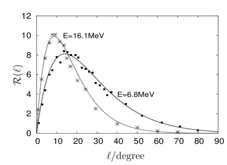
Figure 7: Our fit of the angular resolution ${\cal R}(\ell)$ as a function of $\ell$ for positron energies $E_{e}=6.8$ and 16.1 MeV together with measured points from Ref. Nakahata:1998pz .

The angular resolution ${\cal R}(\ell)d\ell$ is defined as the probability that inside two cones with opening angles $\ell$ and $\ell+d\ell$ around the true direction the reconstructed direction is contained. Reference Nakahata:1998pz gives numerical values for the opening angle $\ell$ of a cone around the true direction which contains 68% of the reconstructed directions as well as the values of ${\cal R}(\ell)$ as a function of $\ell$ for various energies. An inspection by eye shows that ${\cal R}(\ell)$ is characterized by a large tail and cannot be well fitted by a Gaussian distribution. Inspired by the Landau distribution for energy losses, we have found that ${\cal R}(\ell)$ is well described by

$${\cal R}(\ell)={\cal C}\exp\left(-\frac{x+e^{-x}}{2}\right)\sin(\ell)~{},$$ (30)

where ${\cal C}$ is a normalization constant, and

$$x = \frac{\ell}{\sigma}-a\,,$$ (31)

$$a = -0.7E/{\rm MeV}-3.7\,,$$ (32)

$$\vartheta_{\max} = 38^{\circ}\,\sqrt{{\rm MeV}/E}~{},$$ (33)

$$\sigma = [\vartheta_{\max}+\ln(2-\sqrt{3})]/a~{}.$$ (34)

For illustration, we show in Fig. 7 the angular resolution ${\cal R}(\ell)$ as a function of $\ell$ for positron energies $E_{e}=6.8$ and 16.1 MeV as implemented in our simulation, together with the measurements extracted from Nakahata:1998pz .

References

- (1) A. Habig, K. Scholberg, and M. Vagins, poster at Neutrino’98 (unpublished).
-
(2)
K. Scholberg,
“SNEWS: The Supernova early warning system,”
astro-ph/9911359.
See also http:// hep.bu.edu/snnet/ - (3) A. S. Dighe and A. Y. Smirnov, “Identifying the neutrino mass spectrum from the neutrino burst from a supernova,” Phys. Rev. D 62, 033007 (2000) [hep-ph/9907423].
- (4) C. Lunardini and A. Y. Smirnov, “Supernova neutrinos: Earth matter effects and neutrino mass spectrum,” Nucl. Phys. B 616, 307 (2001) [hep-ph/0106149].
- (5) C. Lunardini and A. Y. Smirnov, “Probing the neutrino mass hierarchy and the 13-mixing with supernovae,” [hep-ph/0302033].
- (6) K. Takahashi and K. Sato, “Earth effects on supernova neutrinos and their implications for neutrino parameters,” Phys. Rev. D 66, 033006 (2002) [hep-ph/0110105].
- (7) A. S. Dighe, M. T. Keil and G. G. Raffelt, “Detecting the neutrino mass hierarchy with a supernova at IceCube,” JCAP 0306, 005 (2003) [hep-ph/0303210].
- (8) A. S. Dighe, M. T. Keil and G. G. Raffelt, “Identifying earth matter effects on supernova neutrinos at a single detector,” JCAP 0306, 006 (2003) [hep-ph/0304150].
- (9) E. Waxman and A. Loeb, “TeV neutrinos and GeV photons from shock breakout in supernovae,” Phys. Rev. Lett. 87, 071101 (2001) [astro-ph/0102317].
-
(10)
The INTEGRAL satellite webpage:
http://isdcul3.unige.ch/Public/Integral/integral.html - (11) J. F. Beacom and P. Vogel, “Can a supernova be located by its neutrinos?,” Phys. Rev. D 60, 033007 (1999) [astro-ph/9811350].
- (12) S. Ando and K. Sato, “Determining the supernova direction by its neutrinos,” Prog. Theor. Phys. 107, 957 (2002) [hep-ph/0110187].
- (13) A. Burrows, D. Klein and R. Gandhi, “The future of supernova neutrino detection,” Phys. Rev. D 45, 3361 (1992).
- (14) M. Apollonio et al. [CHOOZ Collaboration], “Determination of neutrino incoming direction in the CHOOZ experiment and its application to supernova explosion location by scintillator detectors,” Phys. Rev. D 61, 012001 (2000) [hep-ex/9906011].
- (15) J. F. Beacom and M. R. Vagins, “GADZOOKS! Antineutrino spectroscopy with large water Cherenkov detectors,” hep-ph/0309300.
- (16) N. I. Fisher, T. Lewis, B. J. J. Embleton, Statistical analysis of spherical data (Cambridge University Press, Cambridge, 1987).
- (17) K. V. Mardia and P. E. Jupp, Directional statistics (John Wiley & Sons, Chichester, 1999).
- (18) C. R. Rao, “Information and accuracy attainable in the estimation of statistical parameters,” Bull. Calcutta Math. Sc. 37, 81 (1945).
- (19) M. Cramér, Mathematical Methods of Statistics (Princeton University Press, Princeton, 1946).
- (20) R. A. Fisher, “The logic of inductive inference,” J. Roy. Stat. Soc. 98, 39 (1935).
- (21) M. Nakahata et al. [Super-Kamiokande Collaboration], “Calibration of Super-Kamiokande using an electron linac,” Nucl. Instrum. Meth. A 421, 113 (1999) [hep-ex/9807027].
- (22) M. G. Kendall and A. Stuart, The Advanced Theory of Statistics, Vol. 2 (Griffin, London, 1969).
- (23) G. G. Raffelt, M. T. Keil, R. Buras, H. T. Janka and M. Rampp, “Supernova neutrinos: Flavor-dependent fluxes and spectra,” astro-ph/0303226.
- (24) T. Totani, K. Sato, H. E. Dalhed and J. R. Wilson, “Future detection of supernova neutrino burst and explosion mechanism,” Astrophys. J. 496, 216 (1998) [astro-ph/9710203].
- (25) M. C. Gonzalez-Garcia and C. Peña-Garay, “Three-neutrino mixing after the first results from K2K and KamLAND,” hep-ph/0306001.
- (26) V. S. Berezinsky and V. S. Ptuskin, “Radiation generated in young type-II supernova envelopes by shock-accelerated cosmic-rays,” Pisma Astr. Zh. 14, 713 (1988) [Soviet Astr. Lett. 14, 304 (1988)].
- (27) E. V. Derishev, F. A. Aharonian, V. V. Kocharovsky and Vl. V. Kocharovsky, “Particle acceleration through multiple conversions from charged into neutral state and back,” astro-ph/0301263.
- (28) C. Spiering, “High Energy Neutrino Astronomy,” Prog. Part. Nucl. Phys. 48, 43 (2002).
- (29) F. Halzen and D. Hooper, “High-energy neutrino astronomy: The cosmic ray connection,” Rept. Prog. Phys. 65, 1025 (2002) [astro-ph/0204527].
- (30) J. Ahrens et al. [IceCube Collaboration], “IceCube: The next generation neutrino telescope at the South Pole,” astro-ph/0209556.
- (31) G. V. Domogatskii, “Status of the BAIKAL neutrino project,” astro-ph/0211571.
- (32) A. Capone et al., “Measurements of light transmission in deep sea with the AC9 transmissometer,” Nucl. Instrum. Meth. A 487, 423 (2002) [astro-ph/0109005]. See also http://nemoweb.lns.infn.it/
-
(33)
D. F. Cowen,
“Results from the Antarctic Muon and Neutrino Detector Array
(AMANDA),”
astro-ph/0211264.
See also http://amanda.berkeley.edu/ -
(34)
E. Aslanides et al. [ANTARES Collaboration],
“A deep sea telescope for high energy neutrinos,”
astro-ph/9907432. See also http://antares.in2p3.fr - (35) E. Anassontzis et al. [NESTOR Collaboration], “Nestor: A Status Report,” Nucl. Phys. Proc. Suppl. 85, 153 (2000). See also http://www.nestor.org.gr
- (36) J. Ahrens [IceCube Collaboration], “Sensitivity of the IceCube detector to astrophysical sources of high energy muon neutrinos,” astro-ph/0305196.
- (37) M. T. Keil, G. G. Raffelt and H. T. Janka, “Monte Carlo study of supernova neutrino spectra formation,” Astrophys. J. 590, 971 (2003) [astro-ph/0208035].
- (38) A. Strumia and F. Vissani, “Precise quasielastic neutrino nucleon cross section,” to appear in Phys. Lett. B [astro-ph/0302055].
- (39) W. C. Haxton, “The nuclear response of water Cherenkov detectors to supernova and solar neutrinos,” Phys. Rev. D 36, 2283 (1987).
- (40) E. Kolbe, K. Langanke and P. Vogel, “Estimates of weak and electromagnetic nuclear decay signatures for neutrino reactions in Super-Kamiokande,” Phys. Rev. D 66, 013007 (2002).
- (41) K. Langanke, P. Vogel and E. Kolbe, “Signal for supernova and neutrinos in water Čerenkov detectors,” Phys. Rev. Lett. 76, 2629 (1996) [nucl-th/9511032].