Abstract

We review the predictions of the theory of Color Glass Condensate for gluon production cross section in p(d)A collisions. We demonstrate that at moderate energies, when the gluon production cross section can be calculated in the framework of McLerran-Venugopalan model, it has only partonic level Cronin effect in it. At higher energies/rapidities corresponding to smaller values of Bjorken $x$ quantum evolution becomes important. The effect of quantum evolution at higher energies/rapidities is to introduce suppression of high-$p_{T}$ gluons slightly decreasing the Cronin enhancement. At still higher energies/rapidities quantum evolution leads to suppression of produced gluons at all values of $p_{T}$.

I Introduction

Recently there has been a surge of interest in particle production in proton-nucleus (pA) and deuteron-nucleus (dA) collisions at high energies. The interest was inspired by the new data produced by the dA program at RHIC [1, 2, 3, 4], which should enable one to separate the contributions of the initial state effects [8] such as parton saturation [9, 10, 11, 12, 13] from the final state effects, such as jet quenching and energy loss in the quark-gluon plasma (QGP) [14, 15, 16, 17], to the suppression of high transverse momentum particles observed in $Au-Au$ collisions at RHIC [5, 6, 7].

Saturation physics has been largely successful in describing hadron multiplicities in Au-Au collisions at RHIC [18]. It can also have important implications for the transverse momentum distributions [19] and particle correlations and azimuthal anisotropies [20]. It has been demonstrated [21] that saturation provides very favorable initial conditions for the thermalization of parton modes with the transverse momenta $k_{T}\sim Q_{s}$, where $Q_{s}$ is the saturation scale. The thermalization was also found [21] to approximately preserve the centrality dependence of total hadron multiplicities determined by the initial conditions [18]. Recent lattice results [22, 23] show that the initial average transverse momentum $\langle k_{T}\rangle$ of the produced partons is $\langle k_{T}\rangle\sim Q_{s}$, which makes the “soft thermalization” scenario preserving the initial centrality and rapidity distributions quite likely. Final state interactions, however, will undoubtedly modify the transverse momentum distributions at $k_{T}\leq(1\div 3)\ Q_{s}$ without introducing new momentum scale [21]. If the produced medium lives long enough, then high $k_{T}$ jets will be suppressed as well because of the jet quenching and energy loss [14, 15, 16, 17].

The first $d-Au$ data from RHIC show Cronin enhancement extending up to $k_{T}\simeq 6$ GeV around $y\sim 0$ [1, 3] whereas at slightly forward rapidity around $y\sim 1$ no significant enhancement is seen [2]. The absence of suppression indicates that final state interactions are indeed responsible for the effect observed in $Au-Au$ collisions [5, 6, 7] in the same $k_{T}$ range. However, the non–universality of the ratios for the charged hadron and $\pi^{0}$ spectra [1] indicate deviations from the independent jet fragmentation up to $k_{T}\simeq 5$ GeV. Similar non-universality in the same $k_{T}$ range was observed for $\Lambda$ and $K$ production [24], and in $p,\bar{p}$ and pion production [25] in $Au-Au$ collisions. It remains to be checked if there is a statistically significant suppression of high $k_{T}$ charged hadron and $\pi^{0}$ yields above the Cronin enhancement region ($k_{T}\geq 6$ GeV), and if this suppression depends on centrality of $d-Au$ collisions. This question is of crucial importance for the interpretation of the spectacular effect observed in $Au-Au$ collisions [5, 6, 7] because this is the kinematical region in which the independent jet fragmentation picture, and thus the perturbative jet quenching description, begin to apply.

The first dA data from RHIC [1, 2, 3] give the ratio of the number of particles produced in a dA collision over the number of particles produced in a pp collision scaled by the number of collisions

$$R^{dA}(k_{T},y)\,=\,\frac{\frac{dN^{dA}}{d^{2}k\ dy}}{N_{coll}\,\frac{dN^{pp}}{d^{2}k\ dy}}.$$ (1)

To understand the new data on $R^{dA}$ and what it implies for our understanding of high energy nuclear wave functions we are going to study here the expectations for $R^{dA}$ from saturation physics. Our approach will be somewhat academic: in this paper, we will not include explicitly all of the effects related to the fact that high-$k_{T}$ of produced particles corresponds to rather large Bjorken $x$ in the actual RHIC experiments at central rapidity – the effective Bjorken $x$ of high-$k_{T}$ ($k_{T}>5$ GeV) particles observed at mid-rapidity at RHIC at $\sqrt{s}=200$ GeV is about $x\approx 0.1$ which may be too large for the small-$x$ treatment that we present here (see [26], but see also [27]). These finite–energy effects have to be accurately accounted for before we can compare our calculations to the data. Nevertheless, we feel that a better understanding of the qualitative features of hadron production within the saturation framework is a necessary pre–requisite for a complete theoretical description of high energy $p(d)-A$ collisions.

We assume that collisions take place at very high energy such that the effective Bjorken $x$ is sufficiently small for all $k_{T}$ of interest. For simplicity we will analyze proton-nucleus collisions assuming that the main qualitative conclusions would be applicable to dA. Since we can not calculate $N_{coll}$ in a model-independent way, we will be using Eq. (34) for our definition of $R^{pA}$, which is identical to Eq. (1) applied to pA collisions with a proper definition of $N_{coll}$ (see [28] for a discussion of uncertainties involved in theoretical evaluations of this quantity).

The problem of gluon production in $pA$ collisions has been solved in the framework of McLerran-Venugopalan model [12] in [29] (see also [30, 31, 32, 33]). The resulting cross section includes the effects of all multiple rescatterings of the produced gluon and the proton in the target nucleus [29]. At higher energy quantum evolution becomes important [34, 35, 36, 37, 38, 39, 40, 41]. In the large $N_{c}$ limit the small-$x$ evolution equation can be written in a non-linear integro-differential form [35, 36, 37, 38] shown here in Eq. (51). The inclusion of non-linear evolution [35, 36, 37, 38] in the quasi-classical gluon production cross section of [29] has been done in [42] (see also [43, 44]). The study of the resulting gluon spectrum and corresponding gluonic $R^{pA}$ is the goal of this paper.

The paper is organized as follows. In Sect. IIA we discuss two main definitions of unintegrated gluon distribution functions: the standard definition (2) and the one inspired by non-Abelian Weizsäcker-Williams field of a nucleus in McLerran-Venugopalan model (7) [12, 13]. We argue, following [42, 45], that the Eq. (7) is the correct definition of the unintegrated gluon distribution counting the number of gluon quanta. We proceed by analyzing $k_{T}$-dependence of the distribution functions. In Sect. IIB we prove the sum rules for both distribution functions given in Eqs. (13) and (14), which are valid in the quasi-classical approximation only. In the framework of McLerran-Venugopalan model [12, 46] the sum rules insure that the presence of shadowing in nuclear gluon distribution functions in the saturation regime ($k_{T}{{}_{\displaystyle{<}}\atop\displaystyle{\sim}}Q_{s0}$) requires enhancement of gluons at higher $k_{T}$ ($k_{T}{{}_{\displaystyle{>}}\atop\displaystyle{\sim}}Q_{s0}$) reminiscent of anti-shadowing. This conclusion is quantified in Sect. IIC [see Fig. 3 and Eqs. (29) and (30)] and the differences between distribution functions are clarified [see Eqs. (24) and (25)]. However, as we demonstrate in Sect. IIB, the sum rules break down once quantum evolution with energy [35, 36, 37, 38] is included. They turn into inequalities (20) and (21). This indicates that, while multiple rescatterings in McLerran-Venugopalan model only redistribute gluons in transverse momentum phase space conserving the total number of gluons in the nucleus [29], quantum evolution of [35, 36, 37, 38] actually reduces the number of gluons in the nuclear wave functions at a given value of Bjorken $x$.

In Sect. III we study the gluon production cross section in pA in the quasi-classical approximation [29]. In Sect. IIIA we show that the gluon production cross section calculated in [29] in McLerran-Venugopalan multiple rescattering model exhibits only Cronin-like enhancement [47], as shown in Fig. 4 and in Eq. (39) (cf. [48, 49]). In the corresponding moderately high energy regime the height and $k_{T}$-position of the Cronin peak are increasing functions of centrality as can be seen from Eq. (40). In Sect. IIIB following [42] we point out that, surprisingly, the gluon production cross section in pA can be written in a $k_{T}$-factorized form (45) [9, 50] with the unintegrated distribution functions defined by Eq. (2), physical meaning of which is less clear than that of Weizsäcker-Williams ones (7). In Sect. IIIB we also prove a sum rule (48) which insures that suppression of produced gluons at low $k_{T}$ ($k_{T}{{}_{\displaystyle{<}}\atop\displaystyle{\sim}}Q_{s0}$) demands Cronin-like enhancement at high $k_{T}$ ($k_{T}{{}_{\displaystyle{>}}\atop\displaystyle{\sim}}Q_{s0}$) in McLerran-Venugopalan model. The relative amounts of suppression and enhancement are different from the quasi-classical gluon distribution case of Sect. II.

Multiple rescatterings of partons inside the nucleus are believed to be the cause of Cronin effect. Phenomenologically these multiple rescatterings are usually modeled by introducing transverse momentum broadening in the nuclear structure functions [51, 52, 53, 54]. In Sect. III we demonstrate how an explicit pQCD calculation of these multiple rescatterings done in [29] yields us Cronin effect (cf. [48, 49]).

Sect. IV is devoted to studying the effects of nonlinear evolution (51) on the gluon production cross section in pA. In Sect. IVA we use the analogy to the case of gluon production in deep inelastic scattering (DIS) solved in [42, 44] to include the effects of evolution (51) in the gluon production cross section in pA. The result is given by Eq. (55). By expanding the all-twist formula (55) we then study the effect of nonlinear evolution on the gluon production at the leading twist (Sect. IVB) and next-to-leading twist (Sect. IVC) level. In Sect. IVB we start by deriving gluon production cross section at the leading twist level (66). We then estimate the cross section for high $k_{T}$ ($k_{T}>k_{\rm geom}\gg Q_{s}(y)$) in the double logarithmic approximation (70) [50] and demonstrate that the corresponding $R^{pA}$ is approaching $1$ at high $k_{T}$ from below, i.e., that $R^{pA}<1$ at $k_{T}\gg Q_{s}(y)$ [see Eq. (79)]. We proceed by evaluating Eq. (66) in the extended geometric scaling region ($Q_{s}(y)<k_{T}\,{{}_{\displaystyle{<}}\atop\displaystyle{\sim}}\,k_{\rm geom}$) [45, 55, 56]. The resulting leading twist gluon production cross section (90) leads to further suppression of gluon production due to the change in gluon anomalous dimension [8] as shown in Eqs. (93) and (95). At very high energies when the gluon production in $pp$ is also in the extended geometric scaling region ($k_{T}<k_{\rm geom}^{p}$) the ratio $R^{pA}$ saturates at $R^{pA}\sim A^{-1/6}$, as follows from Eq. (96). The next-to-leading twist contribution to the gluon production cross section in pA is evaluated in Sect. IVC with the result given by Eqs. (102) and (103). One can see that the subleading twist term contributes towards enhancement of gluon production at high $k_{T}$. However, in the $k_{T}$ region where the next-to-leading twist contribution dominates over higher twists it is small compared to the leading twist term. Therefore the positive sign of the higher twist term can not alter our conclusion of high-$k_{T}$ suppression we derived by analyzing leading twist. To understand how all twists add up we study what happens to Cronin peak ($k_{T}\sim Q_{s}(y)$) at high energy in Sect. IVD. We find that the height of the Cronin maximum decreases with energy and eventually Cronin peak flattens out at the same level as the rest of $R^{pA}$ at higher $k_{T}$, which is shown in Eq. (121). In Sect. IVE we observe that inclusion of evolution only strengthens the suppression of $R^{pA}$ at low $k_{T}$ ($k_{T}\ll Q_{s}(y)$) [see Eq. (124)] which was observed before in Sect. IIIB in the quasi-classical case. In Sect. IVF we construct a toy model illustrating the conclusion of Sect. IV that quantum evolution [35, 36, 37, 38] introduces suppression of $R^{pA}$ at all values of $k_{T}$ (see Fig. 8). We demonstrate that quantum evolution not only suppresses $R^{pA}$ making it less than $1$, but also turns $R^{pA}$ into a decreasing function of collision centrality contrary to the quasi-classical expectations.

We conclude in Sect. V by summarizing our results.

II A Tale of Two Gluon Distribution Functions

A Definitions

There are two different ways to define unintegrated gluon distribution function of a proton or nucleus. The most conventional way relates it to the $q\bar{q}$ dipole cross section on the target nucleus via two gluon exchange. Here we are going to use a similar definition relating the unintegrated gluon distribution to the dipole cross section on the nucleus (see Fig. 1).

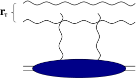
FIG. 1.: “Conventional” definition of unintegrated gluon distribution relating it to the gluon dipole cross section. The exchanged gluon lines can connect to either gluon in the dipole.

The corresponding gluon distribution is given by (cf. [41, 43])

$$\phi(x,\underline{k}^{2})\,=\,\frac{C_{F}}{\alpha_{s}\,(2\pi)^{3}}\,\int d^{2}b\,d^{2}r\,e^{-i{\underline{k}}\cdot{\underline{r}}}\ \nabla^{2}_{r}\,N_{G}({\underline{r}},{\underline{b}},y=\ln 1/x),$$ (2)

where $N_{G}({\underline{r}},{\underline{b}},y=\ln 1/x)$ is the forward amplitude of a gluon dipole of transverse size ${\underline{r}}$ at impact parameter ${\underline{b}}$ and rapidity $y$ scattering on a nucleus [35, 42]. We denote by $\underline{k}$ the transverse components of the four-vector $k$, and by $k_{T}$ its length. The definition of Eq. (2) is inspired by $k_{T}$-factorization and is valid as long as one can neglect multiple rescatterings of the dipole in the nucleus. By using Eq. (2) in the saturation region where higher twists (multiple rescatterings) become important one implicitly assumes that there exists a certain gauge in which the $q\bar{q}$ dipole cross section on a nucleus is given by a two gluon exchange interaction between the dipole and the nucleus and the interaction shown in Fig. 1 is literally all one needs to obtain the correct dipole cross section. It is not clear at present whether this is the case and such a gauge exists. Therefore the gluon distribution given by Eq. (2) does not give one the number of gluons in the nuclear wave function in the saturation region. The applications of the definition (2) will be clarified later.

Another definition of unintegrated gluon distribution literally counts the number of gluons in the nuclear wave function. To construct it in the quasi-classical limit of high energy QCD given by McLerran-Venugopalan model [12] one has to first find the classical gluonic field of the nucleus in the light cone gauge of the ultrarelativistic nucleus (non-Abelian Weizsäcker-Williams field) and then calculate the correlator of two of such fields to get unintegrated gluon distribution function (see Fig. 2).

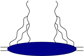
FIG. 2.: Definition of unintegrated gluon distribution in McLerran-Venugopalan model.

The non-Abelian Weizsäcker-Williams field of a nucleus has been found in [13], leading to the following expression for the corresponding gluon distribution [13, 29]

$$\phi^{WW}(x,\underline{k}^{2})\, = \,\frac{1}{2\,\pi^{2}}\,\int d^{2}b\,d^{2}r\,e^{-i{\underline{k}}\cdot{\underline{r}}}\ \mbox{Tr}\left<{\underline{A}}^{WW}({\underline{0}})\cdot{\underline{A}}^{WW}({\underline{r}})\right>\,\rangle$$ (3)

$$= \,\frac{4\,C_{F}}{\alpha_{s}\,(2\pi)^{3}}\,\int d^{2}b\,d^{2}r\,e^{-i{\underline{k}}\cdot{\underline{r}}}\ \frac{1}{{\underline{r}}^{2}}\ (1-e^{-{\underline{r}}^{2}Q_{s0}^{2}\ln(1/r_{T}\Lambda)/4}),$$ (4)

where

$$Q_{s0}^{2}({\underline{b}})\,=\,4\pi\,\alpha_{s}^{2}\,\rho\,T(\underline{b}),$$ (5)

with $\rho$ the atomic number density in the nucleus with atomic number $A$, $T(\underline{b})$ the nuclear profile function and $\Lambda$ some infrared cutoff.

Generalizing Eq. (3) to include non-linear small-$x$ evolution in it [35, 36, 37, 38] is rather difficult. However, the problem of including small-$x$ evolution has been solved for $F_{2}$ structure function and for the gluon production cross section in DIS [35, 42]. Inspired by those examples we conjecture that replacing the Glauber-Mueller [46] forward gluon dipole amplitude on the nucleus by its’ fully evolved expression to be found from the nonlinear evolution equation [35, 38]

$$1-e^{-{\underline{r}}^{2}Q_{s0}^{2}\ln(1/r_{T}\Lambda)/4}\,\,\,\Rightarrow\,\,\,N_{G}({\underline{r}},{\underline{b}},y)$$ (6)

would give us the unintegrated gluon distribution function of a nucleus in the general case:

$$\phi^{WW}(x,\underline{k}^{2})\,=\,\frac{4\,C_{F}}{\alpha_{s}\,(2\pi)^{3}}\,\int d^{2}b\,d^{2}r\,e^{-i{\underline{k}}\cdot{\underline{r}}}\ \frac{1}{{\underline{r}}^{2}}\ N_{G}({\underline{r}},{\underline{b}},y=\ln 1/x).$$ (7)

Similar expression for gluon distribution was obtained earlier in [45].

An important observation concerning the two gluon distributions presented above has been made in [42, 43]. It was shown that, while the Weizsäcker-Williams gluon distribution of Eq. (7) indeed has a clear physical meaning of counting the number of gluons [13], it is the gluon distribution inspired by $k_{T}$-factorization and given by Eq. (2) that enters gluon production cross section in pA collisions and in DIS [42, 43]. More precisely, the gluon production cross section including the effects of multiple rescatterings and quantum evolution in it can be reduced to a $k_{T}$-factorized form [9] with the unintegrated gluon distribution of a nucleus given by Eq. (2) [42]. The authors can not offer any simple physical explanation of this paradox. Nevertheless we keep both distributions in the discussion below keeping in mind that the first one is more relevant to particle production in pA.

B $k_{T}$-dependence: General Arguments

Both definitions of unintegrated gluon distribution (2) and (7) have the same high-$k_{T}$ asymptotics in the quasi-classical approximation (see e.g. Eq. (3)), which reads

$$\phi_{A}(x,\underline{k}^{2})\,=\,\phi^{WW}_{A}(x,\underline{k}^{2})\,=\,A\,\phi_{N}(x,\underline{k}^{2})\,=\,A\,\frac{\alpha_{s}\,C_{F}}{\pi}\,\frac{1}{\underline{k}^{2}},\hskip 28.45274ptk_{T}\rightarrow\infty,$$ (8)

where the index $A$ ($N$) denotes gluon distribution in a nucleus (nucleon). Therefore the distributions are equivalent at the level of leading twist, i.e., as long as we include only a single rescattering in the dipole amplitude $N_{G}$.

In the quasi-classical case of McLerran-Venugopalan model both gluon distributions obey a sum rule which we are going to prove here for $\phi$. From Eq. (2) one can easily infer that

$$\int d^{2}k\,\phi_{A}(x,\underline{k}^{2})\,=\,\frac{C_{F}}{\alpha_{s}\,(2\pi)}\,\int d^{2}b\ \left(\nabla^{2}_{r}\ N_{G}({\underline{r}},{\underline{b}},y=\ln 1/x)\right)\bigg{|}_{{\underline{r}}=0}.$$ (9)

At very small $r_{T}$ the dipole cross section $N_{G}$ in McLerran-Venugopalan model goes to zero as $r_{T}^{2}$ (color transparency [57]) with the coefficient in the front proportional to $A^{1/3}$. One can see that this is explicitly true for the Glauber-Mueller expression for the dipole cross section $N_{G}$ [46]

$$N_{G}({\underline{r}},{\underline{b}},y=0)\,=\,1-e^{-{\underline{r}}^{2}Q_{s0}^{2}\ln(1/r_{T}\Lambda)/4}.$$ (10)

For $N_{G}$ from Eq. (10) we observe that

$$\lim_{r_{T}\rightarrow 0}\left(\nabla^{2}_{r}\ N_{G}({\underline{r}},{\underline{b}},y=0)-A^{1/3}\,\nabla^{2}_{r}\ n_{G}({\underline{r}},{\underline{b}},y=0)\right)\,=\,0$$ (11)

where $n_{G}$ is the gluon dipole cross section on a single nucleon obtained from Eq. (10) by expanding it to the lowest non-trivial order and putting $A=1$. Remembering that

$$\int_{A}d^{2}b\,=\,A^{2/3}\int_{N}d^{2}b$$ (12)

we conclude from Eqs. (9) and (11) that in the quasi-classical approximation (see also [29])

$$\int d^{2}k\,\phi_{A}(y=0,\underline{k}^{2})\,=\,A\,\int d^{2}k\,\phi_{N}(y=0,\underline{k}^{2}).$$ (13)

Similarly one can show that the Weizsäcker-Williams gluon distribution in Eq. (7) obeys the same sum rule in the quasi-classical approximation

$$\int d^{2}k\,\phi^{WW}_{A}(y=0,\underline{k}^{2})\,=\,A\,\int d^{2}k\,\phi^{WW}_{N}(y=0,\underline{k}^{2}).$$ (14)

However, the sum rules of Eqs. (13) and (14) break down when the non-linear evolution with energy [35, 38] is included. To see this we first note that for very small $r_{T}$ one can use the expression for $N_{G}$ given by the double logarithmic approximation [50, 56, 45] (see Sect. IV for details on similar calculations)

$$N_{G}(r_{T}\approx 0,{\underline{b}},y)\,=\,\frac{r_{T}^{2}\,Q_{s0}^{2}}{8\,\sqrt{\pi}}\,\frac{\ln^{1/4}\frac{1}{r_{T}\,Q_{s0}}}{(2\,{\overline{\alpha}}_{s}\,y)^{3/4}}\,e^{2\,\sqrt{2\,{\overline{\alpha}}_{s}\,y\,\ln 1/(r_{T}\,Q_{s0})}}$$ (15)

with

$${\overline{\alpha}}_{s}\,=\,\frac{\alpha_{s}\,N_{c}}{\pi}.$$ (16)

Similarly for the proton amplitude $n_{G}$ we write

$$n_{G}(r_{T}\approx 0,{\underline{b}},y)\,=\,\frac{r_{T}^{2}\,\Lambda^{2}}{8\,\sqrt{\pi}}\,\frac{\ln^{1/4}\frac{1}{r_{T}\,\Lambda}}{(2\,{\overline{\alpha}}_{s}\,y)^{3/4}}\,e^{2\,\sqrt{2\,{\overline{\alpha}}_{s}\,y\,\ln 1/(r_{T}\,\Lambda)}},$$ (17)

where now the scale characterizing the proton is given by

$$\Lambda^{2}\,=\,4\,\pi\,\alpha_{s}^{2}\frac{1}{S_{p}}$$ (18)

with $S_{p}$ the cross sectional transverse area of the proton. Employing the fact that $Q_{s0}^{2}=A^{1/3}\Lambda^{2}$ we can easily see that the amplitudes in Eqs. (15) and (17) do not satisfy the condition of Eq. (11) invalidating the sum rule. In fact using Eqs. (15) and (17) in Eq. (11) gives an inequality

$$\lim_{r_{T}\rightarrow 0}\left(\nabla^{2}_{r}\ N_{G}({\underline{r}},{\underline{b}},y=\ln 1/x)-A^{1/3}\,\nabla^{2}_{r}\ n_{G}({\underline{r}},{\underline{b}},y=\ln 1/x)\right)\,<\,0.$$ (19)

Eq. (19), together with a similar equation for $N_{G}/{\underline{r}}^{2}$ turn the sum rules of Eqs. (13) and (14) into inequalities

$$\int d^{2}k\,\phi_{A}(x,\underline{k}^{2})\,\leq\,A\,\int d^{2}k\,\phi_{N}(x,\underline{k}^{2})$$ (20)

and

$$\int d^{2}k\,\phi^{WW}_{A}(x,\underline{k}^{2})\,\leq\,A\,\int d^{2}k\,\phi^{WW}_{N}(x,\underline{k}^{2}),$$ (21)

where the equality is achieved only in the quasi-classical limit. We conclude that while multiple rescatterings of gluons in McLerran-Venugopalan model preserve the total number of gluons in a nuclear wave function at a given rapidity $y$, the quantum evolution tends reduce the number of gluons in the wave function via gluon mergers [9].

To study nuclear modification of the gluonic wave functions let us define the unintegrated gluon distributions ratios as

$$R_{A}(x,\underline{k}^{2})\,=\,\frac{\phi_{A}(x,\underline{k}^{2})}{A\,\phi_{N}(x,\underline{k}^{2})}\hskip 19.91684pt\mbox{and}\hskip 19.91684ptR_{A}^{WW}(x,\underline{k}^{2})\,=\,\frac{\phi^{WW}_{A}(x,\underline{k}^{2})}{A\,\phi^{WW}_{N}(x,\underline{k}^{2})}.$$ (22)

The sum rules of Eqs. (13) and (14) imply that, in the quasi-classical approximation, if at some $k_{T}$ the distribution function $\phi^{WW}_{A}(y=0,\underline{k}^{2})$ is smaller than $A\,\phi^{WW}_{N}(y=0,\underline{k}^{2})$, then at some other $k_{T}$ it should be bigger than $A\,\phi^{WW}_{N}(y=0,\underline{k}^{2})$. Using the definitions (22) one concludes from Eq. (14) that if $R_{A}^{WW}(y=0,\underline{k}^{2})$ is below $1$ at some $k_{T}$ it is bound to go above $1$ at some other $k_{T}$ (for the same value of $x$). From Eq. (8) we can conclude that

$$R_{A}(y=0,\underline{k}^{2}),\,R_{A}^{WW}(y=0,\underline{k}^{2})\,\rightarrow\,1,\hskip 28.45274ptk_{T}\,\rightarrow\,\infty.$$ (23)

At the same time, when $k_{T}\ll Q_{s0}$ the saturation effects become important driving $\phi^{WW}_{A}(y=0,\underline{k}^{2})$ below $A\,\phi^{WW}_{N}(y=0,\underline{k}^{2})$, or, equivalently, making $R_{A}^{WW}(y=0,\underline{k}^{2})<1$. Therefore, due to the sum rule of Eqs. (13) and (14), somewhere in the region of $k_{T}{{}_{\displaystyle{>}}\atop\displaystyle{\sim}}Q_{s0}$ the ratio $R_{A}^{WW}(y=0,\underline{k}^{2})$ should go above one, which corresponds to enhancement or broadening of the $k_{T}$ distribution of gluons inside the nucleus. The same broadening argument applies to $\phi_{A}(y=0,\underline{k}^{2})$. We have therefore proved that for both gluon distribution functions calculated in McLerran-Venugopalan model the effects of saturation and the sum rule (13),(14), while making $R_{A}(y=0,\underline{k}^{2})<1$ in the infrared, also require an existence of a $k_{T}$-region where $R_{A}(y=0,\underline{k}^{2})$ is above $1$. This conclusion will be quantified in the next Subsection.

The above argument does not apply to the shadowing ratios $R_{A}(x,\underline{k}^{2})$ and $R_{A}^{WW}(x,\underline{k}^{2})$ when the effects of quantum evolution are included. The sum rules (13) and (14) are replaced by inequalities (20) and (21) which only require a reduction of the overall number of gluons in the nuclear wave function at a given rapidity $y$.

C $k_{T}$-dependence: Quasi-Classical Approximation

To investigate the $k_{T}$-dependence of the unintegrated nuclear gluon distributions $\phi^{WW}_{A}(x,\underline{k}^{2})$ and $\phi_{A}(x,\underline{k}^{2})$ more quantitatively and demonstrate the differences of the two distributions let us study them in McLerran-Venugopalan model [12, 13]. For that we take the gluon dipole amplitude in the Glauber-Mueller approximation [46] of Eq. (10). The high-$k_{T}$ asymptotic for both $\phi^{WW}_{A}(x,\underline{k}^{2})$ and $\phi_{A}(x,\underline{k}^{2})$ is given by Eq. (8).

Inside the saturation region ($k_{T}\ll Q_{s0}$) one has

$$\phi(x,\underline{k}^{2})\,\approx\,\frac{2\,C_{F}\,S_{A}}{\alpha_{s}\,(2\pi)^{2}}\,\frac{k_{T}^{2}}{Q_{s0}^{2}},\hskip 28.45274ptk_{T}\ll Q_{s0},$$ (24)

and

$$\phi^{WW}(x,\underline{k}^{2})\,\approx\,\frac{4\,C_{F}\,S_{A}}{\alpha_{s}\,(2\pi)^{2}}\,\ln\frac{Q_{s0}}{k_{T}},\hskip 28.45274ptk_{T}\ll Q_{s0},$$ (25)

where we assumed for simplicity that the nucleus is cylindrical in which case its cross sectional area is $S_{A}=\pi{\cal R}^{2}$ and $Q_{s0}$ is given by Eq. (5) with $\rho\,T(\underline{b})=A/S_{A}$:

$$Q_{s0}^{2}\,=\,\frac{4\pi\,\alpha_{s}^{2}\,A}{S_{A}},\quad\mathrm{cylindrical\;\;nucleus.}$$ (26)

In Eqs. (24) and (25) the difference between the two gluon distribution functions becomes manifest: $\phi^{WW}_{A}(x,\underline{k}^{2})$ keeps increasing (though only logarithmically) as $k_{T}$ decreases, while $\phi_{A}(x,\underline{k}^{2})$ turns over and goes to zero in the infrared. Still for both distribution functions the ratio $R_{A}$ goes to zero as $k_{T}\rightarrow 0$ since to obtain $R_{A}$ one has to divide Eqs. (24) and (25) by $A\phi_{N}(x,\underline{k}^{2})$ from Eq. (8). The sum rules (14) and (13) require a region of enhancement ($R_{A}>1$) at $k_{T}{{}_{\displaystyle{>}}\atop\displaystyle{\sim}}Q_{s0}$. To see that the enhancement really happens one has to calculate the next-to-leading twist correction to the high-$k_{T}$ asymptotic of Eq. (8). This technique has been applied previously for quark production in [58]. One obtains

$$\phi_{A}(x,\underline{k}^{2})\,=\,\frac{C_{F}\,S_{A}\,Q_{s0}^{2}}{\alpha_{s}\,(2\pi)^{2}\,\underline{k}^{2}}\,\left[1+2\,\frac{Q_{s0}^{2}}{\underline{k}^{2}}\left(\ln\frac{\underline{k}^{2}}{4\,\Lambda^{2}}+2\,\gamma-3\right)+\ldots\right],\hskip 28.45274ptk_{T}\rightarrow\infty,$$ (27)

and

$$\phi^{WW}_{A}(x,\underline{k}^{2})\,=\,\frac{C_{F}\,S_{A}\,Q_{s0}^{2}}{\alpha_{s}\,(2\pi)^{2}\,\underline{k}^{2}}\,\left[1+\frac{Q_{s0}^{2}}{\underline{k}^{2}}\left(\ln\frac{k_{T}}{2\,\Lambda}+\gamma-1\right)+\ldots\right],\hskip 28.45274ptk_{T}\rightarrow\infty,$$ (28)

with $\gamma$ the Euler constant. For the ratios $R_{A}$’s this implies

$$R_{A}\,=\,1+2\,\frac{Q_{s0}^{2}}{\underline{k}^{2}}\left(\ln\frac{\underline{k}^{2}}{4\,\Lambda^{2}}+2\,\gamma-3\right)+\ldots$$ (29)

and

$$R_{A}^{WW}\,=\,1+\frac{Q_{s0}^{2}}{\underline{k}^{2}}\left(\ln\frac{k_{T}}{2\,\Lambda}+\gamma-1\right)+\ldots.$$ (30)

Therefore the ratios of gluon distributions approach $1$ from above for both distribution functions at large $k_{T}$. This of course indicates the presence of high-$k_{T}$ enhancement.

FIG. 3.: The ratio $R_{A}$ of unintegrated gluon distributions in the nucleus and in the nucleon. The thin line represents the Weizsäcker-Williams gluon distribution [Eq. (7)] while the thick line correspond to the more conventional one inspired by $k_{T}$-factorization [Eq. (2)].

Qualitative plots of ratio $R_{A}$ for both distribution functions in McLerran-Venugopalan model are shown in Fig. 3. The thin line corresponds to Weizsäcker-Williams gluon distribution $\phi^{WW}_{A}(x,\underline{k}^{2})$ while the thick one represents the $k_{T}$-factorization distribution $\phi_{A}(x,\underline{k}^{2})$. One can see that in accordance with Eqs. (24) and (25) the distribution $\phi_{A}(x,\underline{k}^{2})$ goes to zero faster than $\phi^{WW}_{A}(x,\underline{k}^{2})$ as $k_{T}\rightarrow 0$ in Fig. 3. In agreement with Eqs. (30) and (29) $R_{A}$ for the distribution $\phi_{A}(x,\underline{k}^{2})$ has a stronger high-$k_{T}$ enhancement than $R_{A}^{WW}$ for the distribution $\phi_{A}^{WW}(x,\underline{k}^{2})$.

Finally, let us point out that the function $R_{A}$ ($R_{A}^{WW}$) shown in Fig. 3 will be modified when quantum evolution is included. Due to the inequalities of Eqs. (20) and (21) the total number of gluons will decrease. As we will see below in Sect. IV the effects of quantum evolution is to introduce suppression of gluons at all $k_{T}$.

III Quasi-Classical Approximation: Cronin Effect Only

A Gluon Production in pA

The problem of gluon production in proton-nucleus collisions in the quasi-classical approximation (McLerran-Venugopalan model) has been solved in [29] (see also [30, 33, 31, 32]). For a quark-nucleus scattering the production cross section reads [29]

$$\frac{d\sigma^{pA}}{d^{2}k\ dy}\,=\,\int d^{2}b\,d^{2}x\,d^{2}y \frac{1}{(2\pi)^{2}}\,\frac{\alpha_{s}C_{F}}{\pi^{2}}\,\frac{{\underline{x}}\cdot{\underline{y}}}{{\underline{x}}^{2}{\underline{y}}^{2}}\,e^{-i{\underline{k}}\cdot({\underline{x}}-{\underline{y}})}$$ (32)

$$\times\left(1-e^{-{\underline{x}}^{2}Q_{s0}^{2}\ln(1/x_{T}\Lambda)/4}-e^{-{\underline{y}}^{2}Q_{s0}^{2}\ln(1/y_{T}\Lambda)/4}+e^{-({\underline{x}}-{\underline{y}})^{2}Q_{s0}^{2}\ln(1/(\underline{x}-\underline{y})_{T}\Lambda)/4}\right),$$

which then has to be convoluted with the light cone wave function of a quark in a proton. The saturation scale $Q_{s0}^{2}$ in Eq. (32) is given by Eq. (5). As was shown in [29] in the approximation when the logarithmic dependence of exponential factors in Eq. (32) on the transverse size is neglected, $\underline{x}^{2}\ln(1/x_{T}\Lambda)\approx\underline{x}^{2}$, the $x_{\perp}$ and $y_{\perp}$ integrations in Eq. (32) can be done exactly yielding

$$\frac{d\sigma^{pA}}{d^{2}k\ dy}\,=\,\frac{\alpha_{s}\,C_{F}}{\pi^{2}}\,\int d^{2}b\,\left\{-\frac{1}{{\underline{k}}^{2}}+\frac{2}{{\underline{k}}^{2}}\,e^{-{\underline{k}}^{2}/Q_{s0}^{2}}+\frac{1}{Q_{s0}^{2}}\,e^{-{\underline{k}}^{2}/Q_{s0}^{2}}\,\left[\ln\frac{Q_{s0}^{4}}{4\,\Lambda^{2}{\underline{k}}^{2}}+\mbox{Ei}\left(\frac{{\underline{k}}^{2}}{Q_{s0}^{2}}\right)\right]\right\},$$ (33)

where $\mathrm{Ei}(x)$ is the exponential integral. Our goal is to construct the ratio of the number of gluons produced in a pA collision over the number of gluons produced in a pp collision scaled by the number of collisions

$$R^{pA}(\underline{k},y)\,=\,\frac{\frac{d\sigma^{pA}}{d^{2}k\ dy}}{A\,\frac{d\sigma^{pp}}{d^{2}k\ dy}}.$$ (34)

In the same approximation in which Eq. (33) is derived the gluon production cross section in pp scaled up by $A$ is given by

$$A\,\frac{d\sigma^{pp}}{d^{2}k\ dy}\,=\,\frac{\alpha_{s}\,C_{F}}{\pi^{2}}\,\int_{A}d^{2}b\,\frac{Q_{s0}^{2}}{{\underline{k}}^{4}},$$ (35)

which can be obtained for instance by taking the $k_{T}/Q_{s0}\gg 1$ limit of Eq. (33) and using the fact that $Q_{s0}^{2}\sim A^{1/3}$. For a cylindrical nucleus the impact parameter ${\underline{b}}$ integration would just give a factor of $S_{A}$. Using Eqs. (33) and (35) in Eq. (34) we then obtain

$$R^{pA}(k_{T})\,=\,\frac{{\underline{k}}^{4}}{Q_{s0}^{2}}\,\left\{-\frac{1}{{\underline{k}}^{2}}+\frac{2}{{\underline{k}}^{2}}\,e^{-{\underline{k}}^{2}/Q_{s0}^{2}}+\frac{1}{Q_{s0}^{2}}\,e^{-{\underline{k}}^{2}/Q_{s0}^{2}}\,\left[\ln\frac{Q_{s0}^{4}}{4\,\Lambda^{2}{\underline{k}}^{2}}+\mbox{Ei}\left(\frac{{\underline{k}}^{2}}{Q_{s0}^{2}}\right)\right]\right\}.$$ (36)

The ratio $R^{pA}(k_{T})$ is plotted in Fig. 4 for $\Lambda=0.2\ Q_{s0}$. It clearly exhibits an enhancement at high-$k_{T}$ typical of Cronin effect [47]. Similar conclusions regarding formula (32) have been reached earlier in [48].

It is worth noting that expanding $R^{pA}(k)$ from Eq. (36) in the powers of $Q_{s0}/k_{T}$ (“twists”) yields a series with only positive terms

$$R^{pA}(k_{T})\,=\,1+2\,\frac{Q_{s0}^{2}}{\underline{k}^{2}}+6\,\frac{Q_{s0}^{4}}{\underline{k}^{4}}+24\,\frac{Q_{s0}^{6}}{\underline{k}^{6}}+\ldots\,=\,\sum_{n=0}^{\infty}\,n!\,\left(\frac{Q_{s0}^{2}}{\underline{k}^{2}}\right)^{n}.$$ (37)

The series (37) is divergent, but it is Borel resummable with the sum given by Eq. (36), though not all terms in Eq. (36) can be reconstructed by Borel resummation procedure.

To establish whether inclusion of the correct transverse size dependence in the exponents of Eq. (32) would change the conclusion about Cronin effect let us study the high-$k_{T}$ asymptotic of Eq. (32). A simple calculation yields

$$\frac{d\sigma^{pA}}{d^{2}k\ dy}\,=\,\frac{\alpha_{s}\,C_{F}}{\pi^{2}}\,\int d^{2}b\,\frac{Q_{s0}^{2}}{{\underline{k}}^{4}}\,\left[\left(\ln\frac{{\underline{k}}^{2}}{4\,\Lambda^{2}}+2\,\gamma-1\right)+\right.$$

$$+\left.\frac{Q_{s0}^{2}}{4\,{\underline{k}}^{2}}\,\left(6\,\ln^{2}\frac{{\underline{k}}^{2}}{4\,\Lambda^{2}}-8\,(4-3\gamma)\,\ln\frac{{\underline{k}}^{2}}{4\,\Lambda^{2}}+29+24\,\gamma^{2}-64\,\gamma\right)+\ldots\right],\hskip 28.45274ptk_{T}\rightarrow\infty.$$ (38)

For a cylindrical nucleus, keeping only the leading logarithmic ($\ln\frac{{\underline{k}}^{2}}{\Lambda^{2}}$) terms in the parentheses of Eq. (38) we obtain

$$R^{pA}(k_{T})\,=\,1+\frac{3}{2}\,\frac{Q_{s0}^{2}}{{\underline{k}}^{2}}\,\ln\frac{{\underline{k}}^{2}}{\Lambda^{2}}+\ldots,\hskip 28.45274ptk_{T}\rightarrow\infty$$ (39)

indicating that $R^{pA}$ approaches $1$ from above at high $k_{T}$, which is typical of Cronin enhancement. We therefore conclude that in the framework of the quasi-classical approximation employed in [29] the ratio $R^{pA}$ is less than $1$ at small $k_{T}{{}_{\displaystyle{<}}\atop\displaystyle{\sim}}Q_{s0}$ and has Cronin enhancement at high $k_{T}{{}_{\displaystyle{>}}\atop\displaystyle{\sim}}Q_{s0}$.

FIG. 4.: The ratio $R^{pA}$ for gluons plotted as a function of $k_{T}/Q_{s0}$ in the quasi-classical McLerran-Venugopalan model as found in [29]. The cutoff is $\Lambda=0.2\,Q_{s}$.

As can be seen from Eqs. (36) and (39), the position of Cronin maximum is determined by the saturation scale, such that $k_{\rm max}=\beta\,Q_{s0}$, where $\beta$ is some weakly increasing function of $\ln Q_{s0}/\Lambda$. The height of the maximum is given by $R^{pA}(k_{\rm max})=R^{pA}(\beta\,Q_{s0})$. Substituting $k_{T}=\beta\,Q_{s0}$ in Eq. (36) we observe that the height of Cronin maximum scales like

$$R^{pA}(\beta\,Q_{s0})\,\sim\,\ln\frac{Q_{s0}}{\Lambda}+\mbox{const}\,\sim\,\ln A+\mbox{const}^{\prime}.$$ (40)

Since, for realistic off-central collisions $A$ is replaced by the number of participants $N_{part}$, we conclude from Eq. (40) that in the quasi-classical approximation considered here the $k_{T}$-position and the height of the Cronin peak should increase with centrality of the $pA$ collision.

B $k_{T}$-Factorization

Let us now show that it is possible to rewrite Eq. (32) in a $k_{T}$-factorized form [9, 43, 42]. Repeating the steps outlined in Sect. IV of [42] we first perform one of the transverse coordinate integrations in Eq. (32) rewriting it as

$$\frac{d\sigma^{pA}}{d^{2}k\ dy}\,=\,\frac{1}{2\pi^{2}}\,\frac{\alpha_{s}C_{F}}{\pi}\,\int d^{2}b\,d^{2}z\,e^{-i{\underline{k}}\cdot{\underline{z}}}\,\left[2\,i\,\frac{{\underline{z}}\cdot{\underline{k}}}{{\underline{z}}^{2}{\underline{k}}^{2}}-\ln\frac{1}{z_{T}\Lambda}\right]\,N_{G}({\underline{z}},{\underline{b}},0),$$ (41)

where $N_{G}({\underline{z}},{\underline{b}},0)$ is given by Eq. (10). Using the fact that $N_{G}(z=0,{\underline{b}},0)=0$ we write Eq. (41) as

$$\frac{d\sigma^{pA}}{d^{2}k\ dy}\,=\,\frac{1}{2\pi^{2}}\,\frac{\alpha_{s}C_{F}}{\pi}\,\frac{1}{{\underline{k}}^{2}}\,\int d^{2}b\,d^{2}z\,N_{G}({\underline{z}},{\underline{b}},0)\,\nabla^{2}_{z}\,\left(e^{-i{\underline{k}}\cdot{\underline{z}}}\,\ln\frac{1}{z_{T}\Lambda}\right).$$ (42)

Let us denote the forward scattering amplitude of a gluon dipole of transverse size ${\underline{r}}$ on a single nucleon (proton) integrated over the impact parameter ${\underline{b}}^{\prime}$ of the dipole measured with respect to the proton by

$$\int d^{2}b^{\prime}\,n_{G}({\underline{r}},{\underline{b}}^{\prime},y=0)\,=\,\pi\,\alpha_{s}^{2}\,{\underline{r}}^{2}\,\ln\frac{1}{r_{T}\,\Lambda}.$$ (43)

Eq. (43) is obtained by expanding Eq. (10) at the leading order and taking $A=1$. It corresponds to the two gluon exchange interaction between the dipole and the proton. In the quasi-classical Glauber-Mueller approximation in which Eq. (10) is derived each nucleon exchanges only two gluons with the dipole [46, 13]. Therefore Eq. (43) is a natural reduction of Eq. (10) to a single nucleon case.

With the help of Eq. (43) we rewrite Eq. (42) as [42]

$$\frac{d\sigma^{pA}}{d^{2}k\ dy}\,=\,\frac{C_{F}}{\alpha_{s}\,\pi\,(2\pi)^{3}}\,\frac{1}{{\underline{k}}^{2}}\,\int d^{2}B\,d^{2}b\,d^{2}z\,\nabla^{2}_{z}\,n_{G}({\underline{z}},{\underline{b}}-{\underline{B}},0)\,e^{-i{\underline{k}}\cdot{\underline{z}}}\,\nabla^{2}_{z}\,N_{G}({\underline{z}},{\underline{b}},0).$$ (44)

Now ${\underline{B}}$ is the impact parameter of the proton with respect to the center of the nucleus and ${\underline{b}}$ is the impact parameter of the gluon with respect to the center of the nucleus as shown in Fig. 5.

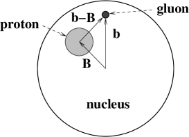
FIG. 5.: Gluon production in pA collisions as seen in the transverse plane. To make the picture easier to read the gluon is placed far away from the proton which is highly unlikely to happen in real life.

Eq. (44) is the expression for gluon production one would write in the $k_{T}$-factorization approach [43]. To see this explicitly let us rewrite Eq. (44) in terms of the unintegrated gluon distribution function from Eq. (2). One easily derives

$$\frac{d\sigma^{pA}}{d^{2}k\ dy}\,=\,\frac{2\,\alpha_{s}}{C_{F}}\,\frac{1}{{\underline{k}}^{2}}\,\int d^{2}q\,\phi_{p}({\underline{q}})\,\phi_{A}({\underline{k}}-{\underline{q}}),$$ (45)

which is the same formula as obtained in $k_{T}$-factorization approach [9, 50, 43]. $\phi_{p}$ is defined as unintegrated gluon distribution of the proton given by Eq. (2) with $n_{G}$ instead of $N_{G}$ on the right hand side. Eq. (45) demonstrates that the gluon production cross section in pA can be expressed in terms of the gluon distribution (2) in a rather straightforward way [42]. Somehow it is the distribution (2) and not the Weizsäcker-Williams distribution (7) that enters Eq. (45).

Eq. (45) demonstrates that, at least in the framework of McLerran-Venugopalan model, the multiple rescattering leading to Cronin enhancement in pA can be incorporated in the gluon distribution functions [29, 33]. There is no clear distinction between the nuclear wave function effects and the Glauber-type rescatterings in the nucleus. Anti-shadowing present in the gluon distribution function $\phi_{A}({\underline{k}})$ as shown in Fig. 3 simply translates into Cronin effect of Fig. 4 via Eq. (45).

In the quasi-classical approximation of McLerran-Venugopalan model one can prove a sum rule for the gluon production cross section in $pA$ similar to the sum rule we proved for gluon distributions in Sect. IIB. To prove the sum rule we note that Eq. (44) implies that

$$\int d^{2}k\,{\underline{k}}^{2}\,\frac{d\sigma^{pA}}{d^{2}k\ dy}\,=\,\frac{C_{F}}{\alpha_{s}\,2\pi^{2}}\,\,\int d^{2}B\,d^{2}b\,\left[\nabla^{2}_{z}\,n_{G}({\underline{z}},{\underline{b}}-{\underline{B}},0)\right]\bigg{|}_{{\underline{z}}=0}\,\left[\nabla^{2}_{z}\,N_{G}({\underline{z}},{\underline{b}},0)\right]\bigg{|}_{{\underline{z}}=0}.$$ (46)

For Glauber-Mueller $N_{G}$ from Eq. (10) and for $n_{G}$ from Eq. (43) the following condition is satisfied

$$\lim_{z_{T}\rightarrow 0}\left\{\left[\nabla^{2}_{z}\,n_{G}({\underline{z}},{\underline{b}}-{\underline{B}},0)\right]\,\left[\nabla^{2}_{z}\,N_{G}({\underline{z}},{\underline{b}},0)\right]-A^{1/3}\left[\nabla^{2}_{z}\,n_{G}({\underline{z}},{\underline{b}}-{\underline{B}},0)\right]\,\left[\nabla^{2}_{z}\,n_{G}({\underline{z}},{\underline{b}},0)\right]\right\}\,=\,0.$$ (47)

The impact parameter integration in pA will give an extra factor of $A^{2/3}$ as compared to pp. Together with Eq. (47) this gives

$$\int d^{2}k\,{\underline{k}}^{2}\,\frac{d\sigma^{pA}_{MV}}{d^{2}k\ dy}\,=\,A\,\int d^{2}k\,{\underline{k}}^{2}\,\frac{d\sigma^{pp}_{MV}}{d^{2}k\ dy}$$ (48)

in the quasi-classical approximation.

Similar to the sum rule proved in Sect. II for gluon distribution functions, the sum rule (48) insures that if the quasi-classical gluon production cross section in pA collisions is, in some region of $k_{T}$, smaller than $A$ times the gluon production cross section in pp than there should be some other region of $k_{T}$ in which their roles are reversed. For $R^{pA}$ defined in Eq. (34) that means that if, in some region of $k_{T}$, it is less than $1$ there must be some other region of $k_{T}$ in which it is greater than $1$. Of course the ${\underline{k}}^{2}$ factors in Eq. (48) make the quantitative amounts of suppression and enhancement very different from the ones dictated by, for instance, the sum rule of Sect. II.

In the quasi-classical approximation for the gluon production in pA considered above $R^{pA}$ is below $1$ at $k_{T}{{}_{\displaystyle{<}}\atop\displaystyle{\sim}}Q_{s0}$. Expanding Eq. (36) for $k_{T}\ll Q_{s0}$ we write

$$R^{pA}(k)\,\approx\,\frac{{\underline{k}}^{2}}{Q_{s0}^{2}}\,\ll\,1\hskip 28.45274pt\mbox{if}\hskip 28.45274ptk_{T}\ll Q_{s0}.$$ (49)

Eq. (49), together with the sum rule (48) imply that there must exist a region of $k_{T}$ with a Cronin-like enhancement of gluon production, which is demonstrated by the full answer plotted in Fig. 4.

IV Including Small-$x$ Evolution: Suppression at all $p_{T}$

A Including Small-$x$ Evolution

As the energy of the collisions increases quantum evolution corrections become important. For produced particles with the same $k_{T}$ higher energy implies smaller effective Bjorken $x$ meaning that the quantum corrections of the type $\alpha_{s}\ln 1/x$ should be resummed. These corrections can be resummed by the BFKL equation [34], which calculates the contribution of the hard (perturbative) pomeron. However, as energy increases multiple pomeron exchanges become important, resulting in a more complicated small-$x$ evolution [39, 40]. In [35, 38] an equation was constructed which resums multiple pomeron exchanges for a forward amplitude of a $q\bar{q}$ dipole scattering on a nucleus in the large $N_{c}$ limit. The forward amplitude $N({\underline{r}},{\underline{b}},Y)$ of a dipole of transverse size ${\underline{r}}$ scattering at impact parameter ${\underline{b}}$ and rapidity $Y$ was normalized such that the total $q{\bar{q}}A$ cross section was given by

$$\sigma^{q{\bar{q}}A}_{tot}\,=\,2\int d^{2}b\,N({\underline{r}},{\underline{b}},Y).$$ (50)

The evolution equation for $N(\underline{r},\underline{b},Y)$ closes only in the large-$N_{c}$ limit of QCD [38, 39] and reads [35, 36, 37]

$$N({\underline{x}}_{01},{\underline{b}},Y)=N({\underline{x}}_{01},{\underline{b}},Y=0)\,e^{-\frac{4\alpha C_{F}}{\pi}\ln\left(\frac{x_{01}}{\rho}\right)Y}+\frac{\alpha C_{F}}{\pi^{2}}\int_{0}^{Y}dy\,e^{-\frac{4\alpha C_{F}}{\pi}\ln\left(\frac{x_{01}}{\rho}\right)(Y-y)}$$

$$\times\int_{\rho}d^{2}x_{2}\frac{x_{01}^{2}}{x_{02}^{2}x_{12}^{2}}\,[2\,N({\underline{x}}_{02},{\underline{b}}+\frac{1}{2}{\underline{x}}_{12},y)-N({\underline{x}}_{02},{\underline{b}}+\frac{1}{2}{\underline{x}}_{12},y)\,N({\underline{x}}_{12},{\underline{b}}+\frac{1}{2}{\underline{x}}_{02},y)],$$ (51)

with the initial condition given by $N({\underline{x}}_{01},{\underline{b}},Y=0)$ taken to be of Mueller-Glauber form [46] in [35]:

$$N({\underline{x}}_{01},{\underline{b}}_{0},Y=0)=1-e^{-{\underline{x}}_{01}^{2}Q_{0s}^{\mathrm{quark}\,2}\ln(1/x_{01T}\Lambda)/4},$$ (52)

where

$$N_{c}\,Q_{0s}^{\mathrm{quark}\,2}\,=\,C_{F}\,Q_{s0}^{2}.$$ (53)

In [42] it was shown how to resum the effects of nonlinear evolution of Eq. (51) for gluon production in DIS. In the quasi-classical approximation the gluon production in DIS is given by a formula similar to Eq. (32) [44]. That formula can also be recast in a $k_{T}$ factorized from of Eq. (44) [42]. As was proven in [42] in order to include quantum evolution (51) in Eq. (44) for DIS one has to make replacements. First, one has to replace $N_{G}({\underline{z}},{\underline{b}},0)$ in Eq. (44) by the forward quark dipole amplitude using the following expression valid in the large-$N_{c}$ limit [42]

$$N_{G}({\underline{z}},{\underline{b}},y)=2N({\underline{z}},{\underline{b}},y)-N({\underline{z}},{\underline{b}},y)^{2},$$ (54)

where $N({\underline{z}},{\underline{b}},y)$ is the forward scattering amplitude of a $q\bar{q}$ dipole on a nucleus evolved by nonlinear equation (51). Then one has to replace $n_{G}({\underline{z}},{\underline{b}},0)$ by $n_{G}({\underline{z}},{\underline{b}},Y-y)$ evolved just by the linear part of Eq. (51) (the BFKL equation [34]). Here $Y$ is the total rapidity interval between the projectile (virtual photon) and target nucleus in a DIS collision. The initial conditions for both $N_{G}$ and $n_{G}$ evolution are given by $N_{G}({\underline{z}},{\underline{b}},0)$ and $n_{G}({\underline{z}},{\underline{b}},0)$ correspondingly.

Since both pA and DIS are considered here as scatterings of an unsaturated projectile (proton or $q\bar{q}$ pair) on a saturated target (nucleus) with the gluon production in the quasi-classical limit given by the same Eq. (44), we may conjecture that inclusion of quantum evolution (51) in gluon production cross section is done similarly for both processes. We therefore write

$$\frac{d\sigma^{pA}}{d^{2}k\ dy}\,=\,\frac{C_{F}}{\alpha_{s}\,\pi\,(2\pi)^{3}}\,\frac{1}{{\underline{k}}^{2}}\,\int d^{2}B\,d^{2}b\,d^{2}z\,\nabla^{2}_{z}\,n_{G}({\underline{z}},{\underline{b}}-{\underline{B}},Y-y)\,e^{-i{\underline{k}}\cdot{\underline{z}}}\,\nabla^{2}_{z}\,N_{G}({\underline{z}},{\underline{b}},y),$$ (55)

where $Y$ is the total rapidity interval between the proton and the nucleus. Just like in DIS $N_{G}$ in Eq. (55) is given by Eq. (54), where $N$ should be found from Eq. (51), while $n_{G}$ should be determined from the linear part of Eq. (55) (BFKL) with the initial conditions given by Eq. (43). Eq. (55) is exact if the proton is modeled as a diquark–quark pair [59], in which case it would be identical to $q\bar{q}$ pair produced by a virtual photon in DIS. In general case Eq. (55) remains a well-motivated conjecture.

Like in Sect. II the sum rule (48) breaks down once non-linear evolution [35, 38] is included in the way shown in Eq. (55). Using the double logarithmic expressions (15) and (17) modifies Eq. (47) into

$$\lim_{z_{T}\rightarrow 0}\left\{\left[\nabla^{2}_{z}\,n_{G}({\underline{z}},{\underline{b}}-{\underline{B}},Y-y)\right]\,\right. \left[\nabla^{2}_{z}\,N_{G}({\underline{z}},{\underline{b}},y)\right]$$ (57)

$$-A^{1/3}\left.\left[\nabla^{2}_{z}\,n_{G}({\underline{z}},{\underline{b}}-{\underline{B}},Y-y)\right]\,\left[\nabla^{2}_{z}\,n_{G}({\underline{z}},{\underline{b}},y)\right]\right\}\,<\,0$$

turning the sum rule of Eq. (48) into an inequality for the cross section from Eq. (55)

$$\int d^{2}k\,{\underline{k}}^{2}\,\frac{d\sigma^{pA}}{d^{2}k\ dy}\,\leq\,A\,\int d^{2}k\,{\underline{k}}^{2}\,\frac{d\sigma^{pp}}{d^{2}k\ dy}.$$ (58)

Again the effect of quantum evolution is to reduce the total number of gluons at a given rapidity, though now it is shown for the case of gluon production weighted by $k_{T}^{2}$. Let us now study in detail how this suppression sets in for various regions of $k_{T}$.

In the following we are going to study effects of evolution equation (51) on the gluon spectrum and on $R^{pA}$. Our goal is to determine whether $R^{pA}$ preserves the shape shown in Fig. 4 with Cronin maximum and low-$k_{T}$ suppression, or quantum evolution would modify this shape introducing extra suppression. Below we will first study the effects of quantum evolution at high-$k_{T}$, $k_{T}{{}_{\displaystyle{>}}\atop\displaystyle{\sim}}Q_{s}$, showing that evolution introduces suppression ($R^{pA}<1$) in that region. We will then proceed by studying the fate of the Cronin peak ($k_{T}\sim Q_{s}$) as evolution sets in. We will show that the Cronin maximum will decrease with the onset of evolution and would eventually disappear. We will then argue that suppression persists for $k_{T}\ll Q_{s}$ when evolution effects are included. We will end the section by constructing a toy model summarizing our conclusions.

To simplify the discussion we will consider a cylindrical nucleus for which Eq. (55) reduces to

$$\frac{d\sigma^{pA}}{d^{2}k\ dy}\,=\,\frac{C_{F}}{\alpha_{s}\,\pi\,(2\pi)^{3}}\,\frac{S_{p}\,S_{A}}{{\underline{k}}^{2}}\,\int d^{2}z\,\nabla^{2}_{z}\,n_{G}({\underline{z}},Y-y)\,e^{-i{\underline{k}}\cdot{\underline{z}}}\,\nabla^{2}_{z}\,N_{G}({\underline{z}},y),$$ (59)

with $S_{p}$ the cross sectional area of the proton.

B Leading Twist Effects

1 Leading Twist Gluon Production Cross Section

We start by exploring the leading high-$k_{T}$ behavior of the gluon spectrum given by Eq. (59). At very high $k_{T}$ the integral in Eq. (59) is dominated by small values of $z_{T}$. Therefore we can neglect the quadratic term in the evolution equation for $N_{G}$ (51) leaving only the linear part – the BFKL evolution with initial conditions for a gluon dipole given by Eq. (10). The corresponding Feynman diagram is shown in Fig. 6. The solution of the BFKL equation is well-known and reads

$$N_{G\,1}({\underline{z}},y)\,=\,\int\frac{d\lambda}{2\pi i}\,C_{\lambda}^{A}\,(z_{T}\,Q_{s0})^{\lambda}\,e^{2\,{\overline{\alpha}}_{s}\,\chi(\lambda)\,y}$$ (60)

with

$$\chi(\lambda)\,=\,\psi(1)-\frac{1}{2}\,\psi\left(1-\frac{\lambda}{2}\right)-\frac{1}{2}\,\psi\left(\frac{\lambda}{2}\right),$$ (61)

${\overline{\alpha}}_{s}$ defined in Eq. (16) and $Q_{s0}$ for a cylindrical nucleus given by Eq. (26). The coefficient $C_{\lambda}^{A}$ is fixed from the initial conditions at $y=0$ given by Eq. (10). Then for small $z_{T}<1/Q_{s0}$

$$C_{\lambda}^{A}\, = \,\sum_{n=1}^{\infty}\,\sum_{m=0}^{n}\,\frac{(-1)^{n+1}}{4^{n}\,(n-m)!\,(2n-\lambda)^{m+1}}\,\ln^{n-m}\frac{Q_{s0}}{\Lambda}$$ (62)

$$= \,\sum_{n=1}^{\infty}\,\frac{1}{4^{n}\,n!\,(\lambda-2n)^{n+1}}\,\left(\frac{Q_{s0}}{\Lambda}\right)^{2n-\lambda}\,\Gamma\left(1+n,\,(2n-\lambda)\,\ln\frac{Q_{s0}}{\Lambda}\right).$$ (63)

Similarly for the gluon dipole cross section on the proton we write

$$n_{G}({\underline{z}},y)\,=\,\int\frac{d\lambda}{2\pi i}\,C_{\lambda}^{p}\,(z_{T}\,\Lambda)^{\lambda}\,e^{2\,{\overline{\alpha}}_{s}\,\chi(\lambda)\,y},$$ (64)

where the scale characterizing the proton $\Lambda$ is given by Eq. (18). The coefficient $C_{\lambda}^{p}$ is obtained by requiring that Eq. (64) reduces to Eq. (43) when $y=0$. For $z_{T}<1/\Lambda$ we derive

$$C_{\lambda}^{p}\,=\,\frac{1}{4\,(\lambda-2)^{2}}.$$ (65)

(We have identified the non-perturbative scale characterizing the proton (18) with the infrared cutoff employed earlier in Eq. (43).)

FIG. 6.: Gluon production in pA collisions at the leading twist level (see text).

Substituting Eqs. (60) and (64) into Eq. (59) and integrating over $\underline{z}$ yields [60, 61]

$$\frac{d\sigma^{pA}}{d^{2}k\ dy}\bigg{|}_{LT}\,=\,\frac{C_{F}\,S_{p}\,S_{A}}{4\,\alpha_{s}\,(2\pi)^{3}}\,\int\frac{d\lambda}{2\pi i}\,\frac{d\lambda^{\prime}}{2\pi i}\,\lambda^{2}\,\lambda^{\prime 2}\,C_{\lambda}^{A}\,C_{\lambda^{\prime}}^{p}\,2^{\lambda+\lambda^{\prime}}\,\frac{\Gamma\left(-1+\frac{\lambda+\lambda^{\prime}}{2}\right)}{\Gamma\left(2-\frac{\lambda+\lambda^{\prime}}{2}\right)}\,\left(\frac{Q_{s0}}{k_{T}}\right)^{\lambda}\,\left(\frac{\Lambda}{k_{T}}\right)^{\lambda^{\prime}}\,$$

$$\times\,e^{2\,{\overline{\alpha}}_{s}\,[\chi(\lambda)\,y+\chi(\lambda^{\prime})\,(Y-y)]}.$$ (66)

Eq. (66) gives the leading twist expression for the gluon production cross section in pA collisions and is illustrated in Fig. 6.

The difference between Eq. (66) and Eq. (13) of [60] is in gamma-functions in the integrand. The difference manifests itself at the order of higher twists, where the gluon distributions used in [60], if taken at $y=0$ and used in inverted Eq. (2) to obtain $n_{p}$, would yield higher twist corrections (higher powers of $r_{T}$) to the right hand side of Eq. (43), which should not be there in the two-gluon exchange approximation corresponding to $y=0$ limit.

2 Double Logarithmic Approximation: Monojet Versus Dijet and First Signs of High-$p_{T}$ Suppression

To derive the high-$k_{T}$ behavior of the gluon production cross section in Eq. (66) we have to evaluate the integrals in it by saddle point method. When $k_{T}\gg Q_{s0},\,\Lambda$ we approximately write

$$\chi(\lambda)\,\approx\,\frac{1}{2-\lambda}.$$ (67)

Then the saddle points are given by

$$\lambda_{sp}\,=\,2-\sqrt{\frac{2\,{\overline{\alpha}}_{s}\,y}{\ln(k_{T}/Q_{s0})}}$$ (68)

and

$$\lambda_{sp}^{\prime}\,=\,2-\sqrt{\frac{2\,{\overline{\alpha}}_{s}\,(Y-y)}{\ln(k_{T}/\Lambda)}}.$$ (69)

Integrating over $\lambda$ and $\lambda^{\prime}$ around the saddle points (68) and (69) in Eq. (66) yields gluon production cross section in double logarithmic approximation (DLA) [50]

$$\frac{d\sigma^{pA}}{d^{2}k\ dy}\bigg{|}_{DLA}\,\approx\,\frac{C_{F}\,S_{p}\,S_{A}}{\alpha_{s}\,(2\pi)^{4}}\,\frac{Q_{s0}^{2}\,\Lambda^{2}}{{\underline{k}}^{4}}\,\frac{1}{2\,{\overline{\alpha}}_{s}}\,\left[\frac{\ln\frac{k_{T}}{Q_{s0}}\,\ln\frac{k_{T}}{\Lambda}}{y^{3}\,(Y-y)^{3}}\right]^{1/4}\,\left(\sqrt{\frac{y}{\ln\frac{k_{T}}{Q_{s0}}}}+\sqrt{\frac{Y-y}{\ln\frac{k_{T}}{\Lambda}}}\right)$$

$$\times\exp\left(2\sqrt{2\,{\overline{\alpha}}_{s}\,y\,\ln\frac{k_{T}}{Q_{s0}}}+2\sqrt{2\,{\overline{\alpha}}_{s}\,(Y-y)\,\ln\frac{k_{T}}{\Lambda}}\ \right).$$ (70)

To understand Eq. (70) let us first construct gluon distribution function

$$xG_{A}(x,Q^{2})\,=\,\int^{Q^{2}}_{\Lambda^{2}}dk^{2}_{T}\,\phi^{A}(x,\underline{k}^{2})$$ (71)

in the same double logarithmic approximation [10]. Using Eq. (60) in Eqs. (2) and (71) we obtain in the double logarithmic approximation

$$xG_{A}(x,Q^{2})\,=\,\frac{C_{F}\,S_{A}\,Q_{s0}^{2}}{\alpha_{s}\,(2\pi)^{3}}\,2\sqrt{\pi}\,\frac{\ln^{1/4}\frac{Q}{Q_{s0}}}{(2\,{\overline{\alpha}}_{s}\,\ln(1/x))^{3/4}}\,e^{2\sqrt{2\,{\overline{\alpha}}_{s}\,\ln(1/x)\,\ln(Q/Q_{s0})}}.$$ (72)

Since the above gluon distribution is obtained in the DLA (large $Q^{2}$) limit of the BFKL equation, it can also be obtained by taking the small-$x$ limit of the DGLAP equation [62]. One can explicitly check that with the help of Eq. (72) and an analogous one for the proton gluon distribution $xG_{p}$, Eq. (70) can be rewritten as

$$\frac{d\sigma^{pA}}{d^{2}k\ dy}\,=\,\frac{2\,\alpha_{s}}{C_{F}\,{\underline{k}}^{2}}\,\left[xG_{p}(x=e^{-Y+y},{\underline{k}}^{2})\,\frac{\partial}{\partial k_{T}^{2}}\,xG_{A}(x=e^{-y},{\underline{k}}^{2})\,+\right.$$

$$\left.+\,xG_{A}(x=e^{-y},{\underline{k}}^{2})\,\frac{\partial}{\partial k_{T}^{2}}\,xG_{p}(x=e^{-Y+y},{\underline{k}}^{2})\right].$$ (73)

Eq. (73) can be obtained directly by using Eq. (72) in Eq. (45) and assuming that the $q$-integration in Eq. (45) is dominated by the regions near ${\underline{q}}=0$ and ${\underline{q}}={\underline{k}}$ [9, 50]. As was shown in detail in [11], Eq. (73) can be reduced to

$$\frac{d\sigma^{pA}}{d^{2}k\ dy}\,=\,\frac{2}{\pi\,N_{c}\,C_{F}}\,\left(\int_{e^{-Y+y}}^{1}\frac{dx_{1}}{x_{1}}\,x_{1}G_{p}(x_{1},{\underline{k}}^{2})\,xG_{A}(x=e^{-y},{\underline{k}}^{2})\,+\right.$$

$$+\left.\int_{e^{-y}}^{1}\frac{dx_{1}}{x_{1}}\,xG_{p}(x=e^{-Y+y},{\underline{k}}^{2})\,x_{1}G_{A}(x_{1},{\underline{k}}^{2})\right)\,\frac{d{\hat{\sigma}}^{gg\rightarrow gg}}{d^{2}k},$$ (74)

which is the standard dijet production cross section derived in collinear factorization approximation (see e.g. [11]). (Of course one of the jets’ momentum in Eq. (74) is integrated over.) Therefore, we have started with a single jet production cross section given by $k_{T}$-factorized expression (66) with BFKL gluon distributions and demonstrated that in the large $k_{T}$ limit it reduces to the conventional dijet production cross section (74) given by collinear factorization with DGLAP-evolved structure functions.

Before we continue let us study $R^{pA}$ given by the cross section of Eq. (70). The naive expectation for the high-$k_{T}$ limit of the leading twist gluon production cross section would be that $R^{pA}=1$. However, already at the level of approximation employed in Eq. (70) this is not quite the case. To see this let us first write down an expression for the gluon production cross section in pp collisions in the leading twist DLA approximation. It is obtained by replacing $Q_{s0}$ and $S_{A}$ in Eq. (70) by $\Lambda$ and $S_{p}$ correspondingly. We obtain

$$\frac{d\sigma^{pp}}{d^{2}k\ dy}\bigg{|}_{DLA}\,\approx\,\frac{C_{F}\,S_{p}^{2}}{\alpha_{s}\,(2\pi)^{4}}\ \frac{\Lambda^{4}}{{\underline{k}}^{4}}\,\frac{1}{2\,{\overline{\alpha}}_{s}}\,\frac{\sqrt{y}+\sqrt{Y-y}}{y^{3/4}\,(Y-y)^{3/4}}\,\exp\left[2\sqrt{2\,{\overline{\alpha}}_{s}\,\ln\frac{k_{T}}{\Lambda}}\left(\sqrt{y}+\sqrt{Y-y}\right)\right].$$ (75)

To calculate $R^{pA}$ we note that since $S_{A}=A^{2/3}S_{p}$ one concludes from Eqs. (26) and (18) that $Q_{s0}^{2}=A^{1/3}\Lambda^{2}$. Using Eqs. (70) and (75) in Eq. (34) yields

$$R^{pA}(k_{T},y)\bigg{|}_{k_{T}\gg Q_{s}}\,=\,\frac{\left(\ln\frac{k_{T}}{Q_{s0}}\,\ln\frac{k_{T}}{\Lambda}\right)^{1/4}}{\sqrt{y}+\sqrt{Y-y}}\,\left(\sqrt{\frac{y}{\ln\frac{k_{T}}{Q_{s0}}}}+\sqrt{\frac{Y-y}{\ln\frac{k_{T}}{\Lambda}}}\right)$$

$$\times\,\exp\left[2\sqrt{2\,{\overline{\alpha}}_{s}\,y}\left(\sqrt{\ln\frac{k_{T}}{Q_{s0}}}-\sqrt{\ln\frac{k_{T}}{\Lambda}}\right)\right],$$ (76)

where $Q_{s}=Q_{s}(y)$ is the full energy dependent saturation scale, which reduces to $Q_{s0}$ at $y=0$. Defining

$$\xi\,\equiv\,\left(\frac{\ln\frac{k_{T}}{Q_{s0}}}{\ln\frac{k_{T}}{\Lambda}}\right)^{1/4}$$ (77)

we rewrite Eq. (76) as

$$R^{pA}(\xi,y)\bigg{|}_{\xi<1}\,=\,\frac{\frac{1}{\xi}\,\sqrt{y}+\xi\,\sqrt{Y-y}}{\sqrt{y}+\sqrt{Y-y}}\,\exp\left[-\,2\,\sqrt{2\,{\overline{\alpha}}_{s}\,y\,\frac{1-\xi^{2}}{1+\xi^{2}}\,\ln\frac{Q_{s0}}{\Lambda}}\,\right]$$ (78)

where $\xi<1$ for $k_{T}>Q_{s0}$, since $Q_{s0}^{2}=A^{1/3}\Lambda^{2}\gg\Lambda^{2}$. For large transverse momenta in question, $k_{T}\gg Q_{s}(y)$, the variable $\xi$ is approaching $1$ from below as is clear from Eq. (77). In the limit $\xi\rightarrow 1$ Eq. (78) becomes

$$R^{pA}(\xi,y)\bigg{|}_{\xi\rightarrow 1}\,\approx\,\left(1+(1-\xi)\frac{\sqrt{y}-\sqrt{Y-y}}{\sqrt{y}+\sqrt{Y-y}}\right)\,\exp\left[-\,2\,\sqrt{2\,{\overline{\alpha}}_{s}\,y\,(1-\xi)\,\ln\frac{Q_{s0}}{\Lambda}}\ \right]$$

$$<\,(2-\xi)\,\exp\left[-\,2\,\sqrt{2\,{\overline{\alpha}}_{s}\,y\,(1-\xi)\,\ln\frac{Q_{s0}}{\Lambda}}\ \right]\,\approx\,\exp\left[-\,2\,\sqrt{2\,{\overline{\alpha}}_{s}\,y\,(1-\xi)\,\ln\frac{Q_{s0}}{\Lambda}}\ \right]\,<\,1,\hskip 8.5359ptk_{T}\gg Q_{s}(y).$$ (79)

We neglected $2-\xi=1+(1-\xi)$ in front of the exponent in Eq. (79) since the $(1-\xi)$ correction to $1$ in it is not enhanced by any parametrically large variables, such as $y$ and $\ln Q_{s0}/\Lambda$ in the exponent. If $R^{pA}(\xi,y)$ from Eq. (79) is expanded in powers of $(1-\xi)$ this prefactor term would give subleading logarithmic corrections to the expansion of the exponent, which are negligible in the DLA limit considered here.

We conclude that $R^{pA}$ from Eq. (76) is smaller than one. Since $R^{pA}(\xi,y)$ in Eq. (79) is an increasing function of $\xi$ and $\xi$ is an increasing function of $k_{T}$, we observe that $R^{pA}(k_{T},y)$ in Eq. (76) is an increasing function of $k_{T}$ approaching $1$ from below. This suppression is mainly due to the difference of the cutoffs in the logarithms of transverse momentum in the exponent of Eq. (76). The cutoff for the nucleus case is given by nuclear saturation scale, which is different from the appropriate scale in a single proton. The high momentum regions, where linear evolution equations work, are cut off from below by saturation scales, which are different for different nuclei and for the proton. In this way, as we can see from Eqs. (76) and (79), saturation influences the physics at high $k_{T}$ as long as corresponding $x_{Bj}$ is small. The effect of saturation is to introduce high-$k_{T}$ suppression.

The suppression of Eq. (79) is a leading twist effect and is due to quantum evolution. In this sense it is similar to the suppression suggested in [8]. However, the suppression of [8] corresponds to a region of lower $k_{T}$, where the double logarithmic approximation of Eq. (76) is not valid any more. There the suppression happens due to the change in anomalous dimension of the gluon distribution function, as we are going to discuss below.

3 Onset of Anomalous Dimension: More High-$p_{T}$ Suppression

For the values of $k_{T}$ lower than considered above (but still much larger than $Q_{s0}$) the saddle point of $\lambda$-integration in Eq. (66) shifts to a smaller value than given by Eq. (68). While in determining the saddle point of Eq. (68) we had to expand $\chi(\lambda)$ around $\lambda=2$, now we have to expand it around $\lambda=1$. There one writes

$$\chi(\lambda)\,\approx\,2\ln 2+\frac{7}{4}\,\zeta(3)\,(\lambda-1)^{2}$$ (80)

obtaining the value of the saddle point

$$\lambda^{*}_{sp}\,=\,1+\frac{\ln\frac{k_{T}}{Q_{s0}}}{7\,\zeta(3)\,{\overline{\alpha}}_{s}\,y}.$$ (81)

As was suggested in [45], the transition of the saddle point from the value given in Eq. (68) to the one given in Eq. (81) happens around

$$k_{\mathrm{geom}}\,\approx\,Q_{s}(y)\,\frac{Q_{s}(y)}{Q_{s0}}$$ (82)

indicating the onset of geometric scaling regime [55]. Here in the double logarithmic approximation the saturation scale depends on energy as [56, 45, 63]

$$Q_{s}(y)\,\approx\,Q_{s0}\,e^{2\,{\overline{\alpha}}_{s}\,y}.$$ (83)

The precise value of the scale $k_{geom}$ in Eq. (82) depends on the definition of the saturation scale and on the way one defines the transition between the double logarithmic and geometric scaling regions. For instance, if we define the transition by equating the saddle points of Eqs. (68) and (81)

$$\lambda_{sp}=\lambda_{sp}^{*},$$ (84)

we get at the point of closest approach (the two saddle point values are never equal to each other)

$$k_{\mathrm{geom}}\,=\,Q_{s0}\,e^{{\overline{\alpha}}_{s}\,y\ 7^{2/3}\zeta(3)^{2/3}2^{-1/3}}\,\approx\,Q_{s0}\,e^{3.28\,{\overline{\alpha}}_{s}\,y}.$$ (85)

When combined with the saturation scale from Eq. (83) this gives

$$k_{\mathrm{geom}}\,\approx\,Q_{s}(y)\,\left(\frac{Q_{s}(y)}{Q_{s0}}\right)^{0.64},$$ (86)

which is slightly different from Eq. (82). At the same time, using the energy dependence of the saturation scale found in [64] in the fixed coupling case

$$Q_{s}(y)\,\approx\,Q_{s0}\,e^{2.44\,{\overline{\alpha}}_{s}\,y}$$ (87)

in Eq. (85) gives

$$k_{\rm geom}\,\approx\,Q_{s}(y)\,\left(\frac{Q_{s}(y)}{Q_{s0}}\right)^{0.34},$$ (88)

which is even lower than Eq. (86). A definition of the transition point different from Eq. (84) would give slightly different estimates for $k_{\rm geom}$.

Nevertheless, the ambiguities in the scale $k_{\rm geom}$ notwithstanding, one can argue, as was done in [45], that there exists a large momentum scale $k_{\rm geom}$, which is parametrically larger than the saturation scale

$$k_{\rm geom}\,\gg\,Q_{s}(y).$$ (89)

For $k_{T}{{}_{\displaystyle{>}}\atop\displaystyle{\sim}}k_{\rm geom}$ there is no geometric scaling and the gluon production is well described by double logarithmic approximation described above resulting in $R^{pA}$ from Eq. (76). $k_{T}{{}_{\displaystyle{<}}\atop\displaystyle{\sim}}k_{\rm geom}$ is the region of geometric scaling [45]. When $k_{T}{{}_{\displaystyle{<}}\atop\displaystyle{\sim}}Q_{s}(y)$ (saturation region) multiple pomeron exchanges become important leading to the saturation of structure functions [9]. For $Q_{s}(y){{}_{\displaystyle{<}}\atop\displaystyle{\sim}}k_{T}{{}_{\displaystyle{<}}\atop\displaystyle{\sim}}k_{\rm geom}$ (extended geometric scaling region) multiple pomeron exchanges are not important yet and the gluon production cross section is described by the leading twist expression in Eq. (66) with the $\lambda$-integral evaluated near the saddle point of Eq. (81) [8].

Performing the $\lambda$ and $\lambda^{\prime}$ integrals in Eq. (66) in the saddle point approximation around the saddle points of Eqs. (81) and (69) correspondingly yields

$$\frac{d\sigma^{pA\,(1)}}{d^{2}k\ dy}\bigg{|}_{LLA}\,\approx\,\frac{C_{F}\,S_{p}\,S_{A}}{\alpha_{s}\,(2\pi)^{4}}\ \frac{Q_{s0}\,\Lambda^{2}}{{\underline{k}}^{3}}\,\frac{C^{A}_{1}}{\sqrt{7\zeta(3)}}\,\frac{\ln^{1/4}\frac{k_{T}}{\Lambda}}{{\overline{\alpha}}_{s}\,(Y-y)^{3/4}\,(2\,{\overline{\alpha}}_{s})^{1/4}}\,$$

$$\times\,\exp\left[{(\alpha_{P}-1)\,y+2\,\sqrt{2\,{\overline{\alpha}}_{s}\,(Y-y)\,\ln\frac{k_{T}}{\Lambda}}-\frac{\ln^{2}\frac{k_{T}}{Q_{s0}}}{14\,\zeta(3)\,{\overline{\alpha}}_{s}\,y}}\right],$$ (90)

where

$$\alpha_{P}-1\,=\,2\,{\overline{\alpha}}_{s}\,\ln 2$$ (91)

is the BFKL pomeron intercept [34] and $C^{A}_{1}$ is well-approximated by the first term in the series of Eq. (62) for all physically reasonable values of $A$

$$C^{A}_{1}\,\approx\,\frac{1}{4}\,\left(1+\ln\frac{Q_{s0}}{\Lambda}\right)\,=\,\frac{1}{4}\,\left(1+\frac{1}{6}\,\ln A\right).$$ (92)

The superscript ⁽¹⁾ in Eq. (90) denotes the leading twist contribution. We assume that in the transverse momentum region where Eq. (90) is valid, $Q_{s}(y){{}_{\displaystyle{<}}\atop\displaystyle{\sim}}k_{T}{{}_{\displaystyle{<}}\atop\displaystyle{\sim}}k_{\rm geom}$, the gluon production cross section in pp collisions is still given by Eq. (75). This is a good approximation since if $k_{T}{{}_{\displaystyle{>}}\atop\displaystyle{\sim}}Q_{s}(y)\gg\Lambda$ the double logarithmic approximation of Eq. (75) should work. Using Eqs. (90) and (75) in Eq. (34) we obtain

$$R^{pA}(k_{T},y)\bigg{|}_{Q_{s}(y){{}_{\displaystyle{<}}\atop\displaystyle{\sim}}k_{T}{{}_{\displaystyle{<}}\atop\displaystyle{\sim}}k_{\rm geom}}\,=\,\frac{k_{T}}{Q_{s0}}\,\frac{2\,C^{A}_{1}}{\sqrt{7\,\zeta(3)}}\,\frac{\ln^{1/4}\frac{k_{T}}{\Lambda}}{(2\,{\overline{\alpha}}_{s})^{1/4}}\,\frac{y^{1/4}}{\sqrt{y}+\sqrt{Y-y}}\,$$

$$\times\,\exp\left[{(\alpha_{P}-1)\,y-2\,\sqrt{2\,{\overline{\alpha}}_{s}\,y\,\ln\frac{k_{T}}{\Lambda}}-\frac{\ln^{2}\frac{k_{T}}{Q_{s0}}}{14\,\zeta(3)\,{\overline{\alpha}}_{s}\,y}}\right].$$ (93)

To determine whether $R^{pA}(k_{T},y)$ in Eq. (93) is greater or less than $1$ we first drop the slowly varying and constant prefactors in front of the exponent and write

$$R^{pA}(k_{T},y)\bigg{|}_{Q_{s}(y){{}_{\displaystyle{<}}\atop\displaystyle{\sim}}k_{T}{{}_{\displaystyle{<}}\atop\displaystyle{\sim}}k_{\rm geom}}\,\sim\,\frac{k_{T}}{Q_{s0}}\,\exp\left[{(\alpha_{P}-1)\,y-2\,\sqrt{2\,{\overline{\alpha}}_{s}\,y\,\ln\frac{k_{T}}{\Lambda}}-\frac{\ln^{2}\frac{k_{T}}{Q_{s0}}}{14\,\zeta(3)\,{\overline{\alpha}}_{s}\,y}}\right]$$ (94)

keeping only parametrically important factors. To estimate the value of $R^{pA}$ in Eq. (94) in the extended geometric scaling region $Q_{s}(y){{}_{\displaystyle{<}}\atop\displaystyle{\sim}}k_{T}{{}_{\displaystyle{<}}\atop\displaystyle{\sim}}k_{\rm geom}$ we substitute $k_{T}=k_{\rm geom}$ into Eq. (94) with $k_{\rm geom}$ from Eq. (82). The result yields an asymptotically small value

$$R^{pA}(k_{T},y)\bigg{|}_{Q_{s}(y){{}_{\displaystyle{<}}\atop\displaystyle{\sim}}k_{T}{{}_{\displaystyle{<}}\atop\displaystyle{\sim}}k_{\rm geom}}\,\sim\,e^{-1.65\,{\overline{\alpha}}_{s}\,y}\,\ll\,1,$$ (95)

where we used $A=197$ for gold nucleus. For other values of $A$ and for other values of $k_{T}$ in the region $Q_{s}(y){{}_{\displaystyle{<}}\atop\displaystyle{\sim}}k_{T}{{}_{\displaystyle{<}}\atop\displaystyle{\sim}}k_{\rm geom}$ one still gets exponential suppression for $R^{pA}(k_{T},y)$. Therefore we conclude that $R^{pA}(k_{T},y)<1$ in the extended geometric scaling region $Q_{s}(y){{}_{\displaystyle{<}}\atop\displaystyle{\sim}}k_{T}{{}_{\displaystyle{<}}\atop\displaystyle{\sim}}k_{\rm geom}$.

As can be checked explicitly, for sufficiently large nucleus (large $A$), $R^{pA}(k_{T},y)$ of Eq. (93) is an increasing function of $k$ for $Q_{s}(y){{}_{\displaystyle{<}}\atop\displaystyle{\sim}}k_{T}{{}_{\displaystyle{<}}\atop\displaystyle{\sim}}k_{\rm geom}$. As $k_{T}$ increases it should smoothly map onto $R^{pA}(k_{T},y)$ of Eq. (76), which would approach $1$ from below for asymptotically high $k_{T}$.

At very high energy the geometric scaling regions for the nucleus and the proton will overlap. Namely, the geometric scale for the proton $k_{\rm geom}^{p}=k_{\rm geom}/A^{1/6}$ will become larger than the saturation scale for the nucleus $Q_{s}(y)$ allowing for a region of $k_{T}$ where anomalous dimension sets in for gluon production both in $pA$ and $pp$. In this asymptotic region one has to estimate the $\lambda$ and $\lambda^{\prime}$ integrals in Eq. (66) around the saddle point given by Eq. (81) (with $\Lambda$ instead of $Q_{s0}$ for the $\lambda^{\prime}$ integral). Replacing Eq. (75) by the appropriate expression where the saddle points of $\lambda$ and $\lambda^{\prime}$ integrals were given by Eq. (81) with $\Lambda$ instead of $Q_{s0}$ we obtain the following asymptotic expression at mid-rapidity ($y=Y/2$)

$$R^{pA}(k_{T},y)\bigg{|}_{Q_{s}(y){{}_{\displaystyle{<}}\atop\displaystyle{\sim}}k_{T}{{}_{\displaystyle{<}}\atop\displaystyle{\sim}}k_{\rm geom}^{p}}\,\sim\,A^{-1/6}\,\exp\left[\frac{\ln^{2}\frac{k_{T}}{\Lambda}-\ln^{2}\frac{k_{T}}{Q_{s0}}}{14\,\zeta(3)\,{\overline{\alpha}}_{s}\,y}\right].$$ (96)

From Eq. (96) we conclude that in the extended geometric scaling region at asymptotically high energies, $R^{pA}$ saturates to a parametrically small lower bound, $R^{pA}\sim A^{-1/6}$, which is independent of energy and is a decreasing function of $A$, or, equivalently, centrality.

To conclude our discussion of high-$k_{T}$ suppression at the leading twist level we note that, as was recently argued in [65], the running coupling effects in the BFKL evolution may modify the $A$-dependence of the saturation scale given by Eqs. (83) and (87), making $Q_{s}(y)$ almost independent of $A$ at very high energy corresponding to large rapidity $y$. This would result in high-$k_{T}$ suppression which would not disappear at any $k_{T}$. That is $R^{pA}(k_{T},y)$ would not approach $1$ anymore at high $k_{T}$. Instead one would have $R^{pA}(k_{T},y)\sim A^{-1/3}$.

C Next-To-Leading Twist

Above we have shown that the effect of quantum evolution (51) on the leading twist gluon production cross section in pA with $k_{T}>Q_{s}(y)$ is to introduce strong suppression of $R^{pA}$. Here we would like to study the effect of evolution on the gluon production at the next-to-leading twist level. Below we are going to show that if one includes the evolution of Eq. (51) into the next-to-leading twist correction to Eq. (66) it would start contributing towards enhancement of $R^{pA}$ at high-$k_{T}$. This appears to indicate that multiple rescatterings always tend to enhance gluon production at high-$k_{T}$. As we will argue later the effect of quantum evolution is much stronger. It dominates at high energies leading to overall suppression of $R^{pA}$.

A perturbative solution of Eq. (51) was constructed in [36] giving the forward amplitude of a $q\bar{q}$ dipole scattering on the nucleus as an expansion in powers of $r_{T}Q_{s}(y)$

$$N({\underline{r}},{\underline{b}},y)\,=\,N_{1}({\underline{r}},{\underline{b}},y)+N_{2}({\underline{r}},{\underline{b}},y)+\ldots,$$ (97)

where the leading behavior of the $n$th term in the series is $N_{n}({\underline{r}},{\underline{b}},y)\sim(r_{T}Q_{s}(y))^{n}$. To find the next-to-leading twist correction to the forward scattering amplitude of a gluon dipole $N_{G}$ we substitute Eq. (97) into Eq. (54) obtaining

$$N_{G}({\underline{r}},{\underline{b}},y)\,=\,2\,N_{1}({\underline{r}},{\underline{b}},y)+2\,N_{2}({\underline{r}},{\underline{b}},y)-[N_{1}({\underline{r}},{\underline{b}},y)]^{2}+\ldots,$$ (98)

where the first term on the right is the leading twist contribution $N_{G\,1}=2\,N_{1}$ given by Eq. (60), and the next two terms shown in Eq. (98) are the next-to-leading twist corrections. Higher twists are not shown in Eq. (98). To calculate the next-to-leading twist correction to gluon forward amplitude

$$N_{G\,2}({\underline{r}},{\underline{b}},y)\,=\,2\,N_{2}({\underline{r}},{\underline{b}},y)-[N_{1}({\underline{r}},{\underline{b}},y)]^{2}\,=\,2\,N_{2}({\underline{r}},{\underline{b}},y)-\frac{1}{4}\,[N_{G\,1}({\underline{r}},{\underline{b}},y)]^{2}$$ (99)

we use $N_{G\,1}$ from Eq. (60) and $N_{2}$ calculated in [36]. Employing Eq. (23) from [36] in Eq. (9a) from the same reference would give us the first term on the right hand side of Eq. (99). In the end we write for a cylindrical nucleus

$$N_{G\,2}({\underline{r}},y)\,=\,-\frac{1}{4}\,\int\frac{d\lambda_{1}\,d\lambda_{2}}{(2\pi i)^{2}}\,C_{\lambda_{1}}^{A}\,C_{\lambda_{2}}^{A}\,(r_{T}\,Q_{s0})^{\lambda_{1}+\lambda_{2}}\,e^{2\,{\overline{\alpha}}_{s}\,y\,[\chi(\lambda_{1})+\chi(\lambda_{2})]}\,$$

$$\times\left(2^{\frac{\lambda_{1}+\lambda_{2}}{2}}\,\frac{\Gamma\left(\frac{\lambda_{1}}{2}\right)\,\Gamma\left(\frac{\lambda_{2}}{2}\right)\,\Gamma\left(1-\frac{\lambda_{1}+\lambda_{2}}{2}\right)}{\Gamma\left(1-\frac{\lambda_{1}}{2}\right)\,\Gamma\left(1-\frac{\lambda_{2}}{2}\right)\,\Gamma\left(\frac{\lambda_{1}+\lambda_{2}}{2}\right)}\,\frac{1}{2[\chi(\lambda_{1})+\chi(\lambda_{2})-\chi(\lambda_{1}+\lambda_{2})]}+1\right).$$ (100)

The slight difference between the factors in the integrands of Eq. (100) and Eq. (23) of [36] is due to different definitions of the coefficients $C^{A}_{\lambda}$ (cf. Eq. (15) of [36] with our Eq. (60)).

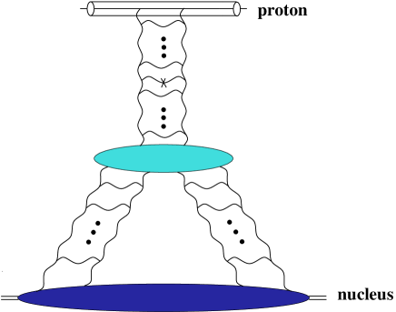
FIG. 7.: Gluon production in pA collisions at the next-to-leading twist level (see text). The blob in the center indicates a triple-pomeron vertex.

The first term in the parentheses of Eq. (100) corresponds to the first term on the right hand side of Eq. (99). When we will substitute $N_{G\,2}$ from Eq. (100) into formula (59) for the cross section, this term would give the contribution illustrated in Fig. 7. It corresponds to the case when the gluon is produced still by the linear evolution with the triple pomeron vertex inserted below the emitted gluon. The rapidity of the triple pomeron vertex was integrated over in arriving at Eq. (100), with only the dominant contribution corresponding to the vertex being right next to the emitted gluon left [36]. (As was shown in [42] the diagrams where the triple pomeron vertex is inserted above the produced gluon cancel in the dipole evolution case considered here [37, 35] in agreement with the expectation of the AGK cutting rules [66].) The second term in the parenthesis of Eq. (100) and on the right hand side of Eq. (99) corresponds to the case where the pomeron splitting occurs precisely at the rapidity position of the gluon production. The emitted gluon is produced by the first step of the non-linear evolution. (This term is the main difference between the results of [42] and [43].) As can be seen in the estimates performed below, this term contributes $50\div 100\%$ of the answer depending on the $k_{T}$-region in question.

Substituting Eq. (100) in Eq. (59) and integrating over ${\underline{z}}$ yields the following contribution to the gluon production cross section at the subleading twist level

$$\frac{d\sigma^{pA}}{d^{2}k\ dy}\bigg{|}_{SLT}=-\frac{C_{F}\,S_{p}\,S_{A}}{\alpha_{s}\,2\,(2\pi)^{3}}\,\int\,\frac{d\lambda_{1}\,d\lambda_{2}\,d\lambda^{\prime}}{(2\pi i)^{3}}\,C_{\lambda_{1}}^{A}\,C_{\lambda_{2}}^{A}\,C_{\lambda^{\prime}}^{p}\,\left(\frac{Q_{s0}}{k_{T}}\right)^{\lambda_{1}+\lambda_{2}}\,\left(\frac{\Lambda}{k_{T}}\right)^{\lambda^{\prime}}$$

$$\times\,e^{2\,{\overline{\alpha}}_{s}\,y\,[\chi(\lambda_{1})+\chi(\lambda_{2})]+2\,{\overline{\alpha}}_{s}\,(Y-y)\,\chi(\lambda^{\prime})}\ 2^{\lambda_{1}+\lambda_{2}+\lambda^{\prime}-3}\ \frac{\Gamma\left(\frac{\lambda_{1}+\lambda_{2}+\lambda^{\prime}}{2}-1\right)}{\Gamma\left(2-\frac{\lambda_{1}+\lambda_{2}+\lambda^{\prime}}{2}\right)}\,(\lambda_{1}+\lambda_{2})^{2}\,\lambda^{\prime 2}$$

$$\times\,\left(2^{\frac{\lambda_{1}+\lambda_{2}}{2}}\,\frac{\Gamma\left(\frac{\lambda_{1}}{2}\right)\,\Gamma\left(\frac{\lambda_{2}}{2}\right)\,\Gamma\left(1-\frac{\lambda_{1}+\lambda_{2}}{2}\right)}{\Gamma\left(1-\frac{\lambda_{1}}{2}\right)\,\Gamma\left(1-\frac{\lambda_{2}}{2}\right)\,\Gamma\left(\frac{\lambda_{1}+\lambda_{2}}{2}\right)}\,\frac{1}{2[\chi(\lambda_{1})+\chi(\lambda_{2})-\chi(\lambda_{1}+\lambda_{2})]}+1\right).$$ (101)

To study the onset of higher twist effects, we are interested in the next-to-leading twist contribution (101) in the region of transverse momenta $k_{T}{{}_{\displaystyle{>}}\atop\displaystyle{\sim}}k_{\rm geom}$. Performing $\lambda_{1}$ and $\lambda_{2}$ integrations in Eq. (101) around the saddle point (68) and performing the $\lambda^{\prime}$ integral in Eq. (101) around the saddle point (69) yields

$$\frac{d\sigma^{pA\,(2)}}{d^{2}k\ dy}\bigg{|}_{DLA}\,\approx\,\frac{C_{F}\,S_{p}\,S_{A}\,\sqrt{\pi}}{\alpha_{s}\,(2\pi)^{5}}\ \frac{Q_{s0}^{4}\,\Lambda^{2}}{{\underline{k}}^{6}}\,\frac{\ln^{1/4}\frac{k_{T}}{\Lambda}\,\ln^{1/2}\frac{k_{T}}{Q_{s0}}}{(2\,{\overline{\alpha}}_{s}\,y)^{3/2}\,(2\,{\overline{\alpha}}_{s}\,(Y-y))^{3/4}}\,\left(2\,\sqrt{\frac{2\,{\overline{\alpha}}_{s}\,y}{\ln\frac{k_{T}}{Q_{s0}}}}+\sqrt{\frac{2\,{\overline{\alpha}}_{s}\,(Y-y)}{\ln\frac{k_{T}}{\Lambda}}}\right)$$

$$\times\,\exp\left[4\,\sqrt{2\,{\overline{\alpha}}_{s}\,y\,\ln\frac{k_{T}}{Q_{s0}}}+2\,\sqrt{2\,{\overline{\alpha}}_{s}\,(Y-y)\,\ln\frac{k_{T}}{\Lambda}}\right].$$ (102)

As one can see from Eq. (102) the next-to-leading twist correction tends to increase gluon production cross section at high-$k_{T}$. In the region of $k_{T}$ where Eq. (102) applies, $k_{T}{{}_{\displaystyle{>}}\atop\displaystyle{\sim}}k_{\rm geom}$, the higher twist corrections are parametrically small and can not change the leading twist suppression of Eq. (78).

To study higher twist effects in the extended geometric scaling region, $Q_{s}(y){{}_{\displaystyle{<}}\atop\displaystyle{\sim}}k_{T}{{}_{\displaystyle{<}}\atop\displaystyle{\sim}}k_{\rm geom}$, we evaluate $\lambda_{1}$ and $\lambda_{2}$ integrals in Eq. (101) around the saddle point (81) and do the $\lambda^{\prime}$ integral around the saddle point (69) obtaining

$$\frac{d\sigma^{pA\,(2)}}{d^{2}k\ dy}\bigg{|}_{LLA}\,\approx\,\frac{2\,C_{F}\,S_{p}\,S_{A}\,\sqrt{\pi}}{\alpha_{s}\,(2\pi)^{5}}\ \frac{Q_{s0}^{2}\,\Lambda^{2}}{{\underline{k}}^{4}}\,\frac{(C^{A}_{1})^{2}}{7\zeta(3)}\,\frac{\ln^{1/4}\frac{k_{T}}{\Lambda}}{{\overline{\alpha}}_{s}\,y\,(2\,{\overline{\alpha}}_{s}\,(Y-y))^{3/4}}\,\left(\sqrt{\frac{2\,{\overline{\alpha}}_{s}\,(Y-y)}{\ln\frac{k_{T}}{\Lambda}}}-\frac{2\,\ln\frac{k_{T}}{Q_{s0}}}{7\,\zeta(3)\,{\overline{\alpha}}_{s}\,y}\right)$$

$$\times\,\exp\left[{2\,(\alpha_{P}-1)\,y+2\,\sqrt{2\,{\overline{\alpha}}_{s}\,(Y-y)\,\ln\frac{k_{T}}{\Lambda}}-\frac{2\,\ln^{2}\frac{k_{T}}{Q_{s0}}}{14\,\zeta(3)\,{\overline{\alpha}}_{s}\,y}}\right].$$ (103)

The sign of Eq. (103) is determined by the sign of the expression in the parenthesis. One can see that for very large $k_{T}$ the expression in the parenthesis can become negative making the overall contribution to the cross section negative. However, Eq. (103) is valid only for $k_{T}{{}_{\displaystyle{<}}\atop\displaystyle{\sim}}k_{\rm geom}$ and, therefore, can not be used at arbitrary high transverse momenta. At lower $k_{T}$ the sign changes and the term in Eq. (103) begins to contribute toward enhancement of $R^{pA}$. The value of $k_{T}$ at which the sign transition takes place depends on the rapidity in question as well as on the atomic number $A$ of the nucleus. To estimate the transition value of $k_{T}$ one has to equate two terms in the parenthesis of Eq. (103). Assuming that $\ln k_{T}/Q_{s0}\gg\ln Q_{s0}/\Lambda$ we obtain

$$k_{0}\,\approx\,k_{\rm geom}\,\left(\frac{\Lambda}{Q_{s0}}\right)^{1/3},$$ (104)

with $k_{\rm geom}$ given by Eq. (85). Therefore, the transition from suppression to enhancement in Eq. (103) happens at $k_{0}$ which is smaller than $k_{\rm geom}$ only by a factor of $A^{-1/18}$, which indicates that the term in Eq. (103) is positive inside most of the extended geometric scaling region contributing to enhancement of gluon production. Here again one should note that Eq. (103) gives us a subleading twist contribution which is parametrically smaller than the leading twist term from Eq. (90) in the $k_{T}$ region at hand ($Q_{s}(y){{}_{\displaystyle{<}}\atop\displaystyle{\sim}}k_{T}{{}_{\displaystyle{<}}\atop\displaystyle{\sim}}k_{\rm geom}$). Eq. (103) is thus unlikely to affect the suppression of $R^{pA}$ observed at the leading twist level in Eqs. (95) and (96).

We conclude by observing that even after inclusion of quantum evolution (51) in the gluon production cross section, multiple rescatterings (higher twists) still tend to enhance gluon production at high-$k_{T}$. In the $k_{T}$ region considered above, $k_{T}>Q_{s}(y)$, these higher twist effects are still parametrically small. In the next Subsection we are going to study the region of $k_{T}$ where all twists become important, $k_{T}\sim Q_{s}(y)$. We will show that the combined effect of all twists is to introduce suppression of the Cronin maximum.

D Flattening of the Cronin peak

We have demonstrated that the effect of quantum evolution (51) is to introduce suppression of $R^{pA}(k_{T},y)$ for $k_{T}{{}_{\displaystyle{>}}\atop\displaystyle{\sim}}Q_{s}(y)$ at the leading twist level. Let us now study what happens to $R^{pA}(k_{T},y)$ at $k_{T}\simeq Q_{s}(y)$ as a result of evolution in energy. We showed in Sect. II that in the quasi-classical approximation the Cronin maximum of the ratio $R^{pA}(\underline{k},y)$ occurs at $k_{T}\simeq Q_{s0}$. In this Subsection we will follow the value of the ratio $R^{pA}(k_{T}=Q_{s},y)$ to higher energies when quantum evolution is important. Since the position of the Cronin maximum is likely to be at $k_{T}\simeq Q_{s}(y)$ even when evolution is included, by studying $R^{pA}(k_{T}=Q_{s},y)$ we are going to study the dependence of the height of the Cronin maximum on energy/rapidity.

The fact that the scattering amplitude is a constant at the saturation scale [63, 56, 64] makes our calculation pretty straightforward. First we assume that Mellin transform of the gluon dipole amplitude obtained from the exact solution to the evolution equation Eq. (51) via Eq. (54) can be written as

$$N_{G}(\underline{z},y)=\int\frac{d\lambda}{2\pi i}\,\left\{\begin{array}[]{c}{\tilde{C}}_{\lambda}^{A}\left[z_{T}\,Q_{s}(y)\right]^{\lambda},\hskip 28.45274ptz_{T}>\frac{1}{k_{\rm geom}};\\ \\ C_{\lambda}^{A}\left(z_{T}\,Q_{s0}\right)^{\lambda}\,e^{2\,{\overline{\alpha}}_{s}\,\chi(\lambda)\,y},\hskip 28.45274ptz_{T}<\frac{1}{k_{\rm geom}}.\end{array}\right.$$ (108)

The form of the solution presented in Eq. (108) assumes geometric scaling of $N_{G}$ down to $z_{T}\simeq 1/k_{\rm geom}$ and a leading twist expression for smaller $z_{T}$ in agreement with the analyses of [45, 64]. Throughout this Subsection we will use the definition of the saturation scale $Q_{s}(y)$ from Eq. (83) and the definition of $k_{\rm geom}$ from Eq. (82). Our physical conclusions will be independent of the choice of definitions for saturation and geometric scales.

Note that all information about the nonlinear evolution (51) is encoded in the function $\tilde{C}_{\lambda}^{A}$ in Eq. (108). Using Eq. (108) in Eq. (59) we can calculate the differential $pA$ gluon production cross section at $k_{T}=Q_{s}(y)$. Since $k_{\rm geom}(y)\gg Q_{s}(y)$ for large $y$ we can set $k_{\rm geom}\rightarrow\infty$ neglecting the $z_{T}<1/k_{\rm geom}$ part of the integral in Eq. (59). This approximation is justified in the Appendix A. We also assume that the dipole amplitude on a proton $n_{G}$ is still given by the leading twist expression (64) around $k_{T}\simeq Q_{s}(y)$, which is a good approximation for a reasonable size nucleus. Substituting the first line of Eq. (108) and Eq. (64) into Eq. (59) we have

$$\frac{d\sigma^{pA}}{d^{2}k\,dy}\bigg{|}_{k_{T}=Q_{s}(y)} = \frac{C_{F}\,S_{p}\,S_{A}\,\Lambda^{2}}{\alpha_{s}\pi(2\pi)^{2}}\int_{0}^{\infty}dz_{T}\,z_{T}\,J_{0}(Q_{s}(y)\,z_{T})\int\,\frac{d\lambda}{2\pi i}\,\frac{d\lambda^{\prime}}{2\pi i}\,C_{\lambda^{\prime}}^{p}\,\tilde{C}_{\lambda}^{A}\,\lambda^{2}\,\lambda^{\prime 2}$$ (110)

$$\times\,(z_{T}\,\Lambda)^{\lambda^{\prime}-2}\,[z_{T}\,Q_{s}(y)]^{\lambda-2}\,\,e^{2\,{\overline{\alpha}}_{s}(Y-y)\chi(\lambda^{\prime})}.$$

Performing the $z_{T}$-integration in Eq. (110) yields

$$\frac{d\sigma^{pA}}{d^{2}k\,dy}\bigg{|}_{k_{T}=Q_{s}(y)}\,=\,\frac{C_{F}\,S_{p}\,S_{A}}{\alpha_{s}\pi(2\pi)^{2}}\int\,\frac{d\lambda}{2\pi i}\,\frac{d\lambda^{\prime}}{2\pi i}\,C_{\lambda^{\prime}}^{p}\,\tilde{C}_{\lambda}^{A}\,\lambda^{2}\,\lambda^{\prime 2}\,2^{\lambda+\lambda^{\prime}-3}\,\frac{\Gamma\left(\frac{\lambda+\lambda^{\prime}}{2}-1\right)}{\Gamma\left(2-\frac{\lambda+\lambda^{\prime}}{2}\right)}$$

$$\times\,\left(\frac{\Lambda}{Q_{s}(y)}\right)^{\lambda^{\prime}}e^{2\,{\overline{\alpha}}_{s}(Y-y)\chi(\lambda^{\prime})}.$$ (111)

It can be seen that all energy/rapidity and almost all atomic number dependence in Eq. (111) is given by the $\lambda^{\prime}$-integral. Since $Q_{s}(y)\gg\Lambda$, the integral over $\lambda^{\prime}$ in Eq. (111) can be evaluated in the double logarithmic approximation around the saddle point of Eq. (69) taken at $k_{T}=Q_{s}(y)$. After that the integral over $\lambda$ carries almost no dynamical information. The result reads

$$\frac{d\sigma^{pA}}{d^{2}k\,dy}\bigg{|}_{k_{T}=Q_{s}(y)}\,=\,\frac{C_{F}\,S_{p}\,S_{A}}{\alpha_{s}\,(2\pi)^{4}}\,\sqrt{\pi}\,{\cal C}_{A}\,\frac{\ln^{1/4}\frac{Q_{s}(y)}{\Lambda}}{[2\,{\overline{\alpha}}_{s}\,(Y-y)]^{3/4}}\,\frac{\Lambda^{2}}{Q_{s}^{2}(y)}\,\exp\left(2\sqrt{2\,{\overline{\alpha}}_{s}\,(Y-y)\,\ln\frac{Q_{s}(y)}{\Lambda}}\right),$$ (112)

where the integration over $\lambda$ gave an unknown function ${\cal C}_{A}$ defined as

$${\cal C}_{A}\,=\,\int\frac{d\lambda}{2\pi i}\,\lambda^{2}\,\tilde{C}_{\lambda}^{A}\,2^{\lambda}\,\frac{\Gamma\left(\frac{\lambda}{2}\right)}{\Gamma\left(1-\frac{\lambda}{2}\right)}.$$ (113)

Here we assume that ${\cal C}_{A}$ is only weakly (at most logarithmically) dependent on $A$, as is true for other coefficients like the one shown in Eq. (92). In case of an “ideal” geometric scaling the coefficient $C_{\lambda}^{A}$ in Eq. (108) would be completely $A$-independent ridding ${\cal C}_{A}$ of all of its $A$-dependence as well.

To construct $R^{pA}$ we take the gluon production cross section in $pp$ from Eq. (75) putting $k_{T}=Q_{s}(y)$. Substituting Eqs. (112) and (75) into Eq. (34) we get

$$R^{pA}(Q_{s}(y),y)\,=\,\sqrt{\pi}\,{\cal C}_{A}\,(2\,{\overline{\alpha}}_{s})^{1/4}\,\frac{y^{3/4}}{\sqrt{y}+\sqrt{Y-y}}\,\ln^{1/4}\left(\frac{Q_{s}(y)}{\Lambda}\right)\,\frac{Q_{s}^{2}(y)}{Q_{s0}^{2}}\,\exp\left(-2\,\sqrt{2\,{\overline{\alpha}}_{s}\,y\,\ln\frac{Q_{s}(y)}{\Lambda}}\right).$$ (114)

The energy and $A$-dependence of Eq. (114) can be found using Eq. (83) and keeping in mind that $Q_{s0}=A^{1/6}\,\Lambda$. Since the definition of the saturation scale (83) is valid up to logarithmic prefactors, we can drop the prefactors in Eq. (114) leaving only

$$R^{pA}(Q_{s}(y),y)\,\propto\,\frac{Q_{s}^{2}(y)}{Q_{s0}^{2}}\,\exp\left(-2\,\sqrt{2\,{\overline{\alpha}}_{s}\,y\,\ln\frac{Q_{s}(y)}{\Lambda}}\right).$$ (115)

(If one defines $Q_{s}(y)$ by taking $N_{G}(z_{T}=1/Q_{s}(y),y)$ in the double logarithmic approximation and requiring that $N_{G}(z_{T}=1/Q_{s}(y),y)=$const [56, 63, 64] the prefactors in Eq. (114) would cancel exactly.) Using Eq. (83) in Eq. (115) yields

$$R^{pA}(Q_{s}(y),y)\,\propto\,\exp\left\{4\,{\overline{\alpha}}_{s}\,y\,\left(1-\sqrt{1+\frac{\ln A^{1/6}}{2\,{\overline{\alpha}}_{s}\,y}}\right)\right\}\,<\,1.$$ (116)

We observe from Eq. (116) that in the course of quantum evolution the Cronin maximum of the ratio $R^{pA}$ decreases with energy until, at very high energy, it saturates at the lowest value $R^{pA}\sim A^{-1/6}$, which is much less than $1$. The height of the Cronin peak is also a decreasing function of collision centrality/atomic number $A$, as can be seen from Eq. (116) .

Applicability of Eq. (116) is restricted by applicability of Eqs. (75) and (112). The latter two equations are valid only in the region where $Q_{s}(y)$ is larger than the geometric scale of the proton: $Q_{s}(y)>k_{\rm geom}/A^{1/6}$ with $k_{\rm geom}$ taken from Eq. (85), since this is where the transition between the saddle points takes place. With the help of Eq. (82) this condition becomes $Q_{s}(y)<A^{1/6}Q_{s0}$. In the kinematic region of extremely high $y$ where this condition is not satisfied anymore, one has to replace Eqs. (112) and (75) by appropriate cross sections evaluated around the saddle point of Eq. (81). To generalize the conclusions presented above to arbitrary high rapidity let us follow Mueller and Triantafyllopoulos [64] and define the saturation scale by requiring that the power of the exponent in the leading twist expression for $N_{G}$ given by (cf. Eq. (60))

$$N_{G\,1}({\underline{z}},y)\,=\,\int\frac{d\lambda}{2\pi i}\,C_{\lambda}^{A}\,e^{2\,{\overline{\alpha}}_{s}\,\chi(\lambda)\,y+\lambda\,\ln(z_{T}\,Q_{s0})}$$

is zero and stationary (its derivative with respect to $\lambda$ is zero) at $z_{T}=1/Q_{s}(y)$. These conditions are satisfied at $\lambda_{0}=1.255$ [64] (our definition of $\chi(\lambda)$ is different from the one used in [64]). Resulting saturation scale is given by Eq. (87). Arguing that the $\lambda$-integral in Eq. (60) is dominated by the saddle point in the exponent we conclude that at $z_{T}=1/Q_{s}(y)$ the gluon dipole amplitude $N_{G}(z_{T}=1/Q_{s}(y),y)$ is approximately constant at large $y$ [64]

$$\int\frac{d\lambda}{2\pi i}\,C_{\lambda}^{A}\,\left(\frac{Q_{s0}}{Q_{s}(y)}\right)^{\lambda}\,e^{2\,{\overline{\alpha}}_{s}\,\chi(\lambda)\,y}\,=\,\int\frac{d\lambda}{2\pi i}\,C_{\lambda}^{A}\,e^{2\,{\overline{\alpha}}_{s}\,\chi(\lambda)\,y+\lambda\,\ln(Q_{s0}/Q_{s}(y))}\,\simeq\,\mbox{constant}(y,A).$$ (117)

Making a similar assumption about the $\lambda^{\prime}$-integral in Eq. (111) taken at mid-rapidity ($y=Y/2$) and remembering that $Q_{s0}=A^{1/6}\,\Lambda$ yields

$$\frac{d\sigma^{pA}}{d^{2}k\,dy}\bigg{|}_{k_{T}=Q_{s}(y),\,y=Y/2}\,\sim\,S_{A}\,A^{-\lambda_{0}/6}\,\sim\,A^{2/3-\lambda_{0}/6}.$$ (118)

Modifying Eq. (66) to give gluon production in $pp$ at $k_{T}=Q_{s}(y)$ also taken at mid-rapidity we obtain

$$\frac{d\sigma^{pp}}{d^{2}k\ dy}\bigg{|}_{k_{T}=Q_{s}(y),\,y=Y/2}\,=\,\frac{C_{F}\,S_{p}^{2}}{4\,\alpha_{s}\,(2\pi)^{3}}\,\int\frac{d\lambda}{2\pi i}\,\frac{d\lambda^{\prime}}{2\pi i}\,\lambda^{2}\,\lambda^{\prime 2}\,C_{\lambda}^{A}\,C_{\lambda^{\prime}}^{p}\,2^{\lambda+\lambda^{\prime}}\,\frac{\Gamma\left(-1+\frac{\lambda+\lambda^{\prime}}{2}\right)}{\Gamma\left(2-\frac{\lambda+\lambda^{\prime}}{2}\right)}$$

$$\times\,\left(\frac{\Lambda}{Q_{s}(y)}\right)^{\lambda+\lambda^{\prime}}\,e^{2\,{\overline{\alpha}}_{s}\,[\chi(\lambda)+\chi(\lambda^{\prime})]\,y}.$$ (119)

Again the $\lambda$- and $\lambda^{\prime}$-integrals in Eq. (119) are dominated by the saddle points at $\lambda_{0}$ giving an energy-independent cross section scaling as

$$\frac{d\sigma^{pp}}{d^{2}k\ dy}\bigg{|}_{k_{T}=Q_{s}(y),\,y=Y/2}\,\sim\,A^{-2\,\lambda_{0}/6}$$ (120)

with atomic number $A$. Combining Eqs. (118) and (120) with Eq. (34) yields

$$R^{pA}(Q_{s}(y),y)\,\propto\,A^{-1/3+\lambda_{0}/6}\,\mbox{constant}(y)\,\sim\,A^{-0.124},$$ (121)

for $\lambda_{0}=1.255$. Note that the power of $A$ in Eq. (121) is pretty close to that following from Eq. (116) and the two powers would be identical for $\lambda_{0}=1$. Note also that taking the expression for $R^{pA}$ in the geometric scaling region from Eq. (96) and extrapolating it down to $k_{T}=Q_{s}(y)$ one would obtain a power of $A$ very close to that in Eq. (121) if one uses $Q_{s}(y)$ from Eq. (83). This conclusion not only verifies the self-consistency of our analysis, but also demonstrates that at asymptotic energies the height of Cronin maximum becomes (parametrically) equal to the height of the rest of the $R^{pA}$ curve in the extended geometric scaling region. This is likely to indicate that at these energies the curve flattens out and the Cronin peak disappears.

With the help of Eq. (121) we conclude that at high rapidities/energies the Cronin maximum decreases with energy and centrality, with $R^{pA}(Q_{s}(y),y)$ becoming less than $1$. Eventually, at very high energy, the Cronin peak flattens out and saturates to an energy independent lower limit given by Eq. (121), which is parametrically suppressed by powers of $A$.

E Suppression Deep Inside Saturation Region

Above we have shown that non-linear evolution (51) introduces suppression of gluon production in $pA$ collisions making $R^{pA}<1$ for $k_{T}{{}_{\displaystyle{>}}\atop\displaystyle{\sim}}Q_{s}(y)$. In the region of smaller $k_{T}$, $k_{T}\ll Q_{s}(y)$, we observed in Sect. IIIB that in the quasi-classical case of McLerran-Venugopalan model the ratio $R^{pA}\ll 1$ (see Eq. (49)). When the quantum evolution (51) is included it makes sense to consider the interval of low $k_{T}$ bounded from below by the saturation scale of the proton $\Lambda_{s}(y)$, such that $\Lambda_{s}(y)\ll k_{T}\ll Q_{s}(y)$. (For $k_{T}{{}_{\displaystyle{<}}\atop\displaystyle{\sim}}\Lambda_{s}(y)$ the proton wave function also saturates and particle production in both $pp$ and $pA$ becomes similar to the case of $AA$, which has not been resolved even at the quasi-classical level [22, 23, 33]. Inclusion of evolution in $AA$ is an even more difficult problem which we are not going to address here.) If $k_{T}$ is larger than the geometric scale of the proton $k_{\rm geom}/A^{1/6}$ (but still much less than $Q_{s}(y)$) we can use Eq. (75) to describe the gluon production cross section in $pp$. Deep inside the saturation region in $pA$ the gluon production has been estimated in [42]. Employing Eq. (57) from [42] together with Eq. (75) we conclude that at mid-rapidity

$$R^{pA}(k_{\rm geom}^{p}<k_{T}\ll Q_{s}(y),y)\,\sim\,\frac{k_{T}^{2}}{Q_{s0}^{2}}\,e^{-2\sqrt{2\,{\overline{\alpha}}_{s}\,y\,\ln k_{T}/\Lambda}}.$$ (122)

Eq. (122) shows that inclusion of quantum evolution only introduces more suppression into $R^{pA}$ at $k_{T}\ll Q_{s}(y)$, making it a decreasing function of both the atomic number and energy. At very high energy $k_{T}$ may become smaller than the geometric scale for the proton $k_{\rm geom}/A^{1/6}$ and the gluon production in $pp$ would be driven by the saddle point (81) with $\Lambda$ instead of $Q_{s0}$. Similarly to how it was done in [42] for DLA, one can estimate the gluon production cross section (59) deep inside the saturation region with the dipole amplitude on the proton evaluated around the LLA saddle point $\lambda^{\prime}\approx 1$. The result at mid-rapidity yields

$$R^{pA}(\Lambda_{s}(y)\ll k_{T}\leq k_{\rm geom}^{p})\,\sim\,A^{-1/3}\,\frac{Q_{s}(y)}{\Lambda}\,\exp\left[-(\alpha_{P}-1)y+\frac{2\,\ln^{2}(k_{T}/\Lambda)-\ln^{2}(Q_{s}(y)/\Lambda)}{14\,\zeta(3)\,{\overline{\alpha}}_{s}\,y}\right].$$ (123)

Therefore, at very high energies the ratio $R^{pA}$ becomes almost independent of $k_{T}$ even at very low $k_{T}$. Using the saturation scale from Eq. (83) in Eq. (123) at asymptotic energies gives

$$R^{pA}(\Lambda_{s}(y)\ll k_{T}\leq k_{\rm geom}^{p})\,\sim\,A^{-0.2}\,e^{-1.0\,{\overline{\alpha}}_{s}\,y}.$$ (124)

We observe again that nonlinear evolution leaves $R^{pA}$ very small at $k_{T}\ll Q_{s}(y)$. $R^{pA}$ given by Eq. (124) is a decreasing function of both rapidity/energy and centrality. This conclusion seems natural, since the saturation effects are known to soften the low-$k_{T}$ gluon spectra in pA compared to pp.

F Toy Model

To illustrate the conclusions reached above let us construct a simple toy model exhibiting suppression of $R^{pA}$ at all $k_{T}$. We start with the quasi-classical formula for gluon production in $pA$ in the following form which could be obtained from Eq. (42) for a cylindrical nucleus and for azimuthally symmetric $N_{G}$

$$\frac{d\sigma^{pA}}{d^{2}k\ dy}\,=\,\frac{\alpha_{s}C_{F}}{\pi^{2}}\,\frac{S_{A}}{k_{T}^{2}}\,\int_{0}^{\infty}\,dz_{T}\,J_{0}(k_{T}\,z_{T})\,\ln\frac{1}{z_{T}\Lambda}\ \partial_{z_{T}}\,[z_{T}\ \partial_{z_{T}}N_{G}(z_{T},y=0)].$$ (125)

With the increase of energy the gluon dipole amplitude on the nucleus will reach saturation. Therefore, its $z_{T}$-dependence will change more significantly than for the corresponding amplitude on the proton, which will stay unsaturated. (Of course at very high energy the dipole amplitude on the proton will also reach saturation, but we are not going to consider that energy range here.) Therefore, in our toy model we will assume for simplicity that the gluon dipole amplitude on the proton remains unchanged with increasing energy, giving $\ln 1/(z_{T}\Lambda)$ in Eq. (125). We will model the gluon dipole amplitude at high energy by a Glauber-like unitary expression

$$N_{G}^{toy}(z_{T},y)\,=\,1-e^{-z_{T}\,Q_{s}(y)},$$ (126)

which mimics the onset of anomalous dimension $\lambda=1$ by the linear term in the exponent. The saturation scale $Q_{s}(y)$ in Eq. (126) is some increasing function of $y$ which can be taken from Eq. (83) or from Eq. (87). Indeed the amplitude in Eq. (126) has an incorrect small-$z_{T}$ behavior, scaling proportionally to $z_{T}$ instead of $z_{T}^{2}$ as shown in Eq. (15). If Eq. (126) is used in Eq. (125) it would lead to an incorrect high-$k_{T}$ behavior of the resulting cross section. We therefore argue that Eq. (126) is, probably, a reasonable model for $N_{G}$ inside the saturation and extended geometric scaling regions ($1/z_{T}\sim k_{T}<k_{\rm geom}$), but should not be used for very small $z_{T}$ / high $k_{T}$ ($1/z_{T}\sim k_{T}>k_{\rm geom}$).

Substituting Eq. (126) into Eq. (125) and integrating over $z_{T}$ yields

$$\frac{d\sigma^{pA}_{toy}}{d^{2}k\ dy}\,=\,\frac{\alpha_{s}C_{F}}{\pi^{2}}\,\frac{S_{A}}{k_{T}^{2}}\,\frac{Q_{s}}{k_{T}^{2}+Q_{s}^{2}}\,\left[-\,Q_{s}(k_{T}^{2}+Q_{s}^{2})+\sqrt{k_{T}^{2}+Q_{s}^{2}}\left(2Q_{s}^{2}+\gamma\,k_{T}^{2}+k_{T}^{2}\,\ln\frac{2(k_{T}^{2}+Q_{s}^{2})}{k_{T}\,\Lambda}\right.\right.$$

$$\left.\left.+\frac{k_{T}^{2}}{2}\,\ln\frac{\sqrt{k_{T}^{2}+Q_{s}^{2}}-Q_{s}}{\sqrt{k_{T}^{2}+Q_{s}^{2}}+Q_{s}}\right)\right],$$ (127)

where $\gamma$ is the Euler’s constant and $Q_{s}=Q_{s}(y)$. Corresponding gluon production cross section for $pp$ is obtained by expanding Eq. (127) to the lowest order at high $k_{T}$ and substituting $\Lambda$ instead of $Q_{s}$ and $S_{p}$ instead of $S_{A}$:

$$\frac{d\sigma^{pp}_{toy}}{d^{2}k\ dy}\,=\,\frac{\alpha_{s}C_{F}}{\pi^{2}}\,\frac{S_{p}\,\Lambda}{k_{T}^{3}}\,\left(\ln\frac{2\,k_{T}}{\Lambda}+\gamma\right).$$ (128)

Of course in Eq. (128) one implicitly assumes that anomalous dimension has set in for only one of the protons in $pp$. This assumption is not valid at mid-rapidity, but may be used to study particle production at rapidities near fragmentation region of one of the protons.

Substituting Eqs. (127) and (128) in Eq. (34) yields

$$R^{pA}_{toy}(k_{T},y)\,=\,\frac{k_{T}\,\Lambda}{Q_{s}\,(k_{T}^{2}+Q_{s}^{2})\,(\ln(2\,k_{T}/\Lambda)+\gamma)}\,\left[-\,Q_{s}(k_{T}^{2}+Q_{s}^{2})+\sqrt{k_{T}^{2}+Q_{s}^{2}}\left(2Q_{s}^{2}+\gamma\,k_{T}^{2}\right.\right.$$

$$\left.\left.+k_{T}^{2}\,\ln\frac{2(k_{T}^{2}+Q_{s}^{2})}{k_{T}\,\Lambda}+\frac{k_{T}^{2}}{2}\,\ln\frac{\sqrt{k_{T}^{2}+Q_{s}^{2}}-Q_{s}}{\sqrt{k_{T}^{2}+Q_{s}^{2}}+Q_{s}}\right)\right],$$ (129)

in which we assumed that $\Lambda$ is the saturation scale of the proton such that $Q_{s}^{2}=A^{1/3}\,\Lambda^{2}$ even at high energy.

FIG. 8.: The ratio $R^{pA}$ plotted as a function of $k_{T}/Q_{s}$ for (i) McLerran-Venugopalan model, which is valid for moderate energies (upper solid line); (ii) our toy model for very high energies/rapidities from Eq. (129) (lower solid line); (iii) an interpolation to intermediate energies (dash-dotted and dashed lines). The cutoff is $\Lambda=0.3\,Q_{s}$.

The toy model $R^{pA}_{toy}(k_{T},y)$ from Eq. (129) is plotted as a function of $k_{T}/Q_{s}$ in Fig. 8 for $\Lambda=0.3\,Q_{s}$ (lower solid curve). It exhibits suppression of gluon production in $pA$ at all values of $k_{T}$ leveling off at $R^{pA}_{toy}\sim\Lambda/Q_{s}\sim A^{-1/6}$ for $k_{T}{{}_{\displaystyle{>}}\atop\displaystyle{\sim}}Q_{s}$ at high energy, in agreement with our conclusions of Sections IIIB and IIID.

Our toy model (129) represents the high energy asymptotics of $R^{pA}$. To compare it to lower energies, we also plot $R^{pA}$ for the quasi-classical McLerran-Venugopalan model given by Eq. (36) (upper solid curve in Fig. 8). As the energy increases the upper solid line in Fig. 8 would decrease eventually turning into the lower solid line. The corresponding intermediate energy stages are shown by the dash-dotted and dashed lines in Fig. 8. These lines are for illustrative purposes only and do not correspond to any toy model. They demonstrate how the Cronin peak gradually disappears as energy or rapidity increase.

V Conclusions

In this paper we have demonstrated that saturation effects in the gluon production in pA at moderate energy can be taken into account in the quasi-classical framework of McLerran-Venugopalan model, which includes Glauber-Mueller multiple rescatterings, resulting only in Cronin enhancement of produced gluons at $k_{T}=(1\div 2)\,Q_{s0}$, as was shown in Fig. 4 and in Eq. (39). Similar conclusions have been reached in [48]. In this quasi-classical approximation the height and position of the Cronin peak are increasing functions of centrality as indicated by Eq. (40).

We have also shown that at higher energies/rapidities, when quantum evolution becomes important, it introduces suppression of gluons produced in pA collisions at all values of $k_{T}$, as compared to the number of gluons produced in pp collisions scaled up by the number of collisions $N_{coll}$, as suggested previously [8]. The resulting $R^{pA}$ at high energy/rapidity is a decreasing function of centrality. We have considered three different complimentary regions of $k_{T}$, which cover together all of $k_{T}$-range:

1. $k_{T}>Q_{s}(y)$ region. Gluon production cross section in $pA$ is dominated by the leading twist effects in this region of $k_{T}$. We have shown how the leading twist suppression arises in the double logarithmic approximation for $k_{T}>k_{\rm geom}\gg Q_{s}(y)$ with the corresponding $R^{pA}(k_{T},y)$ given by Eq. (76), which approaches $1$ as $k_{T}\rightarrow\infty$. At $Q_{s}(y)<k_{T}{{}_{\displaystyle{<}}\atop\displaystyle{\sim}}k_{\rm geom}$ the leading twist suppression is mainly due to the change in anomalous dimension $\lambda$ from its double logarithmic value (68) to the leading logarithmic value (81). $R^{pA}(k_{T},y)$ for this $k_{T}$-window is given by Eq. (93) leading to suppression described by Eq. (95). At very high energies, when the extended geometric scaling regions of the proton and the nucleus overlap (for $Q_{s}(y)<k_{T}{{}_{\displaystyle{<}}\atop\displaystyle{\sim}}k_{\rm geom}^{p}$) the decrease of $R^{pA}$ with energy stops at roughly $R^{pA}\sim A^{-1/6}$ as follows from Eq. (96). This leading twist effect has been originally pointed out in [8]. We have not considered suppression mechanisms that may stem from running of the coupling constant, which would modify the $A$-dependence of the saturation scale [65].

2. $k_{T}\sim Q_{s}(y)$ is the position of the Cronin maximum in the quasi-classical approximation. We began the analysis of this $k_{T}$-region by studying higher twists in the adjacent region of $k_{T}>Q_{s}(y)$. Next-to-leading twist term was shown to contribute towards enhancement of $R^{pA}$ at high-$k_{T}$ even when evolution is included. However, higher twist effects are parametrically small at $k_{T}>Q_{s}(y)$ and can not change our leading twist conclusions about suppression. To assess the contribution of all twists we studied the behavior of the Cronin maximum ($k_{T}\sim Q_{s}(y)$) with increasing energy. We showed that $R^{pA}$ at $k_{T}=Q_{s}(y)$ is a decreasing function of energy/rapidity and centrality saturating at the energy-independent lower bound given by Eq. (121). Since the height of the Cronin maximum becomes parametrically of the same order as the rest of $R^{pA}$ at higher $k_{T}$ given by Eq. (96), we conclude that Cronin peak disappears at asymptotically high energies/rapidities.

3. $k_{T}\ll Q_{s}(y)$ region. The suppression of $R^{pA}$ deep inside the saturation region, $k_{T}\ll Q_{s}(y)$, only gets stronger as the evolution (51) is included (see Eq. (124)).

Our results are summarized in Fig. 8.

It is interesting to observe that the behavior of $R^{pA}$ at high energies is qualitatively different from what one would expect by taking the quasi-classical expression (36) and letting $Q_{s}$ in it increase with energy. In case of DIS a similar trick where one replaces $Q_{s0}$ in the Glauber-Mueller expression for the dipole cross section (10) by the energy dependent $Q_{s}$ from, for instance, Eq. (83) leads to correct qualitative behavior of resulting $F_{2}$ structure function and even generates some successful phenomenology [67]. However, as we showed above, a naive generalization of McLerran-Venugopalan model by increasing $Q_{s}$ with energy does not work for $R^{pA}$ even at the qualitative level.

The analysis in the paper was, of course, done for sufficiently high energy and/or rapidity, such that the saturation approach was assumed to be still valid for the highest $k_{T}$ involved. This implies that the effective Bjorken $x$ is still sufficiently small for all $k_{T}$ we consider. The extent to which this treatment applies at high $k_{T}$ hadron production at RHIC is difficult to assess theoretically. We thus eagerly await the results of the experimental analyses of centrality dependence of hadron production above the Cronin region ($k_{T}\geq 6$ GeV). It is also very important to extend the present measurements away from the central rapidity region to separate initial state effects from possible energy loss in cold nuclear matter. Indeed, in the deuteron fragmentation region, the effects of saturation in the $Au$ wave function will be enhanced, while the density of the produced particles (see, e.g., the predictions in [68]) and thus the associated energy loss will be minimal. In the $Au$ fragmentation region the opposite will be true.

We, therefore, conclude that if the effects of quantum evolution and anomalous dimension are observed in the forward rapidity region of $dAu$ collisions at RHIC, they would manifest themselves by reducing $R^{dA}$ at all $k_{T}$ as shown in Fig. 8, eliminating the Cronin enhancement. $R^{dA}$ will become a decreasing function of centrality. The $pA$ program at LHC would observe an even stronger suppression of $R^{pA}$. However, it might be that the quantum evolution effects are still not important even in the forward region of $dAu$ collisions at RHIC. Then reduction of $R^{dA}$ going from mid-rapidity to deuteron fragmentation region should be rather mild and the Cronin peak would not disappear in the forward region. The relevant particle production physics would be described by McLerran-Venugopalan model. The height of the Cronin peak would then be an increasing function of centrality.

If the forthcoming data on $R^{dA}$ in the forward rapidity region of $dAu$ collisions would have no high-$p_{T}$ suppression and would exhibit only a strong Cronin maximum which is an increasing function of centrality in agreement with predictions of multiple rescattering models described in Sect. III [48, 49, 51, 52, 53, 54], then all of the observed high-$p_{T}$ suppression in $Au-Au$ collisions would have to be attributed to the final state effects. However, if the future $R^{dA}$ data in the forward rapidity region exhibits suppression either for all $p_{T}$ or at high $p_{T}$ with $R^{dA}$ being a decreasing function of centrality as described in this paper (see also [8]), then a fraction of $R^{AA}$ suppression in the forward rapidity region of $Au-Au$ collisions should be attributed to initial state quantum evolution effects. Indeed, there is some evidence [4] that the high $k_{T}$ suppression in $Au-Au$ collisions increases between the pseudo–rapidities $\eta=0$ and $\eta=2.2$.

The $dAu$ data at $y\simeq 0$ [1, 2, 3, 4] also suggest suppression of the yields of charged hadrons [3] and neutral pions [1] at $k_{T}\geq 6$ GeV, though the suppression is not significant statistically. If this initial–state effect is confirmed, it should also be taken into account in the interpretation of $Au-Au$ results at $y\simeq 0$.

The $dAu$ results will thus allow to clarify the relative importance of initial and final state interactions at different transverse momenta and rapidities of the produced particles. They will be indispensable for establishing a complete physical picture of heavy ion collisions at RHIC energies.

Note added: After the first version of this paper appeared, a similar analysis has been done in [69, 70, 71]. The analyses of [69, 70, 71] agree with our conclusions on the presence of Cronin effect in the quasi-classical approximation. The results of [69, 71] are also in agreement with our conclusion about high-$p_{T}$ suppression of gluon production.

A

Here we are going to derive Eq. (110). In writing down Eq. (110) we assumed that the integration region $z_{T}<1/k_{\rm geom}$ is negligible. To justify this approximation let us start by substituting Eq. (108) into Eq. (59). We find

$$\frac{d\sigma^{pA}}{d^{2}k\,dy}\bigg{|}_{k_{T}=Q_{s}(y)} = \frac{C_{F}\,S_{p}\,S_{A}}{\alpha_{s}\pi(2\pi)^{2}\,Q_{s}^{2}(y)}\,\bigg{\{}\int_{0}^{1/k_{\rm geom}}dz_{T}\,z_{T}\,J_{0}(Q_{s}(y)z_{T})\int\,\frac{d\lambda}{2\pi i}\int\,\frac{d\lambda^{\prime}}{2\pi i}\,C_{\lambda^{\prime}}^{p}\,C_{\lambda}^{A}\,\lambda^{2}\,\lambda^{\prime 2}\,\Lambda^{2}\,Q_{s0}^{2}$$ (A4)

$$\times\,(z_{T}\,\Lambda)^{\lambda^{\prime}-2}\,(z_{T}\,Q_{s0})^{\lambda-2}\,e^{2\,{\overline{\alpha}}_{s}\,y\,\chi(\lambda)+2\,{\overline{\alpha}}_{s}\,(Y-y)\,\chi(\lambda^{\prime})}$$

$$+\int_{1/k_{\rm geom}}^{\infty}dz_{T}\,z_{T}\,J_{0}(Q_{s}(y)z_{T})\int\,\frac{d\lambda}{2\pi i}\int\,\frac{d\lambda^{\prime}}{2\pi i}\,C_{\lambda^{\prime}}^{p}\,\tilde{C}_{\lambda}^{A}\,\lambda^{2}\,\lambda^{\prime 2}\,\Lambda^{2}\,Q_{s}^{2}(y)$$

$$\times\,(z_{T}\,\Lambda)^{\lambda^{\prime}-2}\,[z_{T}\,Q_{s}(y)]^{\lambda-2}\,e^{2\,{\overline{\alpha}}_{s}\,(Y-y)\,\chi(\lambda^{\prime})}\bigg{\}}.$$

The difference between Eq. (A4) and the target Eq. (110) is

$$\frac{C_{F}\,S_{p}\,S_{A}}{\alpha_{s}\pi(2\pi)^{2}\,Q_{s}^{2}(y)}\,\int_{0}^{1/k_{\rm geom}}dz_{T}\,z_{T}^{-3}\,J_{0}(Q_{s}(y)z_{T})\,\int\,\frac{d\lambda}{2\pi i}\int\,\frac{d\lambda^{\prime}}{2\pi i}\,C_{\lambda^{\prime}}^{p}\,\lambda^{2}\,\lambda^{\prime 2}$$

$$\times\,(z_{T}\,\Lambda)^{\lambda^{\prime}}\,e^{2\,{\overline{\alpha}}_{s}\,(Y-y)\,\chi(\lambda^{\prime})}\,\bigg{[}C_{\lambda}^{A}\,(z_{T}\,Q_{s0})^{\lambda}\,e^{2\,{\overline{\alpha}}_{s}\,y\,\chi(\lambda)}-\tilde{C}_{\lambda}^{A}\,[z_{T}\,Q_{s}(y)]^{\lambda}\bigg{]}.$$ (A5)

Since $k_{\rm geom}\gg Q_{s}(y)$ we can neglect the argument of the Bessel function in the integral in Eq. (A5) putting $J_{0}(0)=1$. Integration over $z_{T}$ then yields

$$\frac{C_{F}\,S_{p}\,S_{A}}{\alpha_{s}\pi(2\pi)^{2}}\,\int\,\frac{d\lambda}{2\pi i}\,\int\,\frac{d\lambda^{\prime}}{2\pi i}\,C_{\lambda^{\prime}}^{p}\,\lambda^{2}\,\lambda^{\prime 2}\,e^{2\,{\overline{\alpha}}_{s}\,(Y-y)\,\chi(\lambda^{\prime})}$$

$$\times\,\frac{1}{\lambda+\lambda^{\prime}-2}\,\left(\frac{\Lambda}{k_{\rm geom}}\right)^{\lambda^{\prime}}\,\frac{k_{\rm geom}^{2}}{Q_{s}^{2}(y)}\,\bigg{[}C_{\lambda}^{A}\,e^{2\,{\overline{\alpha}}_{s}\,y\,\chi(\lambda)}\,\left(\frac{Q_{s0}}{k_{\rm geom}}\right)^{\lambda}-\tilde{C}_{\lambda}^{A}\,\left(\frac{Q_{s}(y)}{k_{\rm geom}}\right)^{\lambda}\bigg{]}.$$ (A6)

Due to the inequality $k_{\rm geom}\gg Q_{s}(y)\gg\Lambda$, the integration over $\lambda^{\prime}$ in Eq. (A6) is dominated by the saddle point at $\lambda^{\prime}\approx 2$, as shown in Eqs. (67) and (69). The integral over $\lambda$ in Eq. (A6) becomes

$$\int\frac{d\lambda}{2\pi i}\,\frac{\lambda^{2}}{\lambda+\lambda^{\prime}-2}\,\left[C_{\lambda}^{A}\,e^{2\,{\overline{\alpha}}_{s}\,y\,\chi(y)}\,\left(\frac{Q_{s0}}{k_{\rm geom}}\right)^{\lambda}\,-\,\tilde{C}_{\lambda}^{A}\,\left(\frac{Q_{s}(y)}{k_{\rm geom}}\right)^{\lambda}\right]$$ (A7)

$$\approx \int\frac{d\lambda}{2\pi i}\,\lambda\,\left[C_{\lambda}^{A}\,e^{2\,{\overline{\alpha}}_{s}\,y\,\chi(y)}\,\left(\frac{Q_{s0}}{k_{\rm geom}}\right)^{\lambda}\,-\,\tilde{C}_{\lambda}^{A}\,\left(\frac{Q_{s}(y)}{k_{\rm geom}}\right)^{\lambda}\right]$$ (A8)

$$= -\frac{\partial}{\partial\ln k_{\rm geom}}\,\left[N_{G}(z_{T}\rightarrow(1/k_{\rm geom})^{-},y)\,-\,N_{G}(z_{T}\rightarrow(1/k_{\rm geom})^{+},y)\right]\,=\,0,$$ (A9)

where we assumed that $N_{G}(\underline{z},y)$ and its derivatives with respect to $z_{T}$ from Eq. (108) are smooth functions of $z_{T}$ such that the difference of the above limits is zero. This assumption is justified since $N_{G}(\underline{z},y)$ is proportional to the scattering matrix which is an analytic function of its variables. Eq. (51) makes $N_{G}(\underline{z},y)$ analytic by construction.

We showed that the difference between the exact Eq. (A4) and our Eq. (110) is zero, making the two equations equal, as desired. However, the above proof required that the representation of $N_{G}(\underline{z},y)$ given by Eq. (108) has a smooth matching of the two regions at $z_{T}=1/k_{\rm geom}$, i.e., that representation (108) is not just a good approximation but an exact identity. To show that no such assumption is required to prove that the expression in Eq. (A6) is a negligible correction to Eq. (110) let us estimate the energy dependence the first term in Eq. (A6). The second term in Eq. (A6) is negative and can only make the overall contribution smaller. Employing double logarithmic approximation for $\lambda$- and $\lambda^{\prime}$-integrals and using Eqs. (83) and (82) we derive (setting $y=Y/2$ for simplicity)

$$\int\,\frac{d\lambda}{2\pi i}\int\,\frac{d\lambda^{\prime}}{2\pi i}\,C_{\lambda^{\prime}}^{p}\,\lambda^{2}\,\lambda^{\prime 2}\,e^{2\,{\overline{\alpha}}_{s}\,(Y-y)\,\chi(\lambda^{\prime})}\,\frac{1}{\lambda+\lambda^{\prime}-2}\,\left(\frac{\Lambda}{k_{\rm geom}}\right)^{\lambda^{\prime}}\frac{k_{\rm geom}^{2}}{Q_{s}^{2}(y)}\,C_{\lambda}^{A}\,e^{2\,{\overline{\alpha}}_{s}\,y\,\chi(\lambda)}\left(\frac{Q_{s0}}{k_{\rm geom}}\right)^{\lambda}$$

$$\propto\,\frac{\Lambda^{2}\,Q_{s0}^{2}\,A^{1/6\sqrt{2}}}{k_{\rm geom}^{2}\,Q_{s}^{2}(y)}\,e^{8\,\sqrt{2}\,{\overline{\alpha}}_{s}\,y}\,\propto\,A^{-\frac{1}{3}+\frac{1}{6\sqrt{2}}}\,e^{-4\,{\overline{\alpha}}_{s}\,y(3-2\sqrt{2})},$$ (A10)

which is a decreasing function of rapidity and centrality. It is obviously negligible compared to the increasing function of $y$ given by Eq. (112). This accomplishes our proof of Eq. (110).

REFERENCES

- [1] S. S. Adler [PHENIX Collaboration], arXiv:nucl-ex/0306021.
- [2] B. B. Back [PHOBOS Collaboration], arXiv:nucl-ex/0306025.
- [3] J. Adams [STAR Collaboration], arXiv:nucl-ex/0306024.
- [4] I. Arsene et al. [BRAHMS Collaboration], Phys. Rev. Lett. 91, 072305 (2003) [arXiv:nucl-ex/0307003].
- [5] K. Adcox et al. [PHENIX Collaboration], Phys. Lett. B 561, 82 (2003) [arXiv:nucl-ex/0207009]; S. S. Adler et al. [PHENIX Collaboration], arXiv:nucl-ex/0304022.
- [6] B. B. Back et al. [PHOBOS Collaboration], arXiv:nucl-ex/0302015.
- [7] J. Adams et al. [STAR Collaboration], arXiv:nucl-ex/0305015; C. Adler et al. [STAR Collaboration], Phys. Rev. Lett. 89, 202301 (2002) [arXiv:nucl-ex/0206011].
- [8] D. Kharzeev, E. Levin and L. McLerran, Phys. Lett. B 561, 93 (2003) [arXiv:hep-ph/0210332].
- [9] L. V. Gribov, E. M. Levin and M. G. Ryskin, Phys. Rept. 100, 1 (1983).
- [10] A. H. Mueller and J. w. Qiu, Nucl. Phys. B 268, 427 (1986).
- [11] J. P. Blaizot and A. H. Mueller, Nucl. Phys. B 289, 847 (1987).
- [12] L. D. McLerran and R. Venugopalan, Phys. Rev. D 49, 2233 (1994) [arXiv:hep-ph/9309289]; Phys. Rev. D 49, 3352 (1994) [arXiv:hep-ph/9311205]; Phys. Rev. D 50, 2225 (1994) [arXiv:hep-ph/9402335].
- [13] Y. V. Kovchegov, Phys. Rev. D 54, 5463 (1996) [arXiv:hep-ph/9605446]; Phys. Rev. D 55, 5445 (1997) [arXiv:hep-ph/9701229]; J. Jalilian-Marian, A. Kovner, L. D. McLerran and H. Weigert, Phys. Rev. D 55, 5414 (1997) [arXiv:hep-ph/9606337].
- [14] J. D. Bjorken, FERMILAB-PUB-82-059-THY (unpublished).
- [15] X. N. Wang, M. Gyulassy and M. Plumer, Phys. Rev. D 51, 3436 (1995) [arXiv:hep-ph/9408344]; M. Gyulassy, P. Levai and I. Vitev, Phys. Rev. Lett. 85, 5535 (2000) [arXiv:nucl-th/0005032]; M. Gyulassy, I. Vitev, X. N. Wang and B. W. Zhang, arXiv:nucl-th/0302077; M. Gyulassy, I. Vitev and X. N. Wang, Phys. Rev. Lett. 86, 2537 (2001) [arXiv:nucl-th/0012092]; I. Vitev and M. Gyulassy, Phys. Rev. Lett. 89, 252301 (2002) [arXiv:hep-ph/0209161]; X. N. Wang, arXiv:nucl-th/0305010.
- [16] R. Baier, Y. L. Dokshitzer, A. H. Mueller, S. Peigne and D. Schiff, Nucl. Phys. B 483, 291 (1997) [arXiv:hep-ph/9607355]; Nucl. Phys. B 484, 265 (1997) [arXiv:hep-ph/9608322]; Nucl. Phys. B 478, 577 (1996) [arXiv:hep-ph/9604327]; R. Baier, Y. L. Dokshitzer, A. H. Mueller and D. Schiff, Phys. Rev. C 58, 1706 (1998) [arXiv:hep-ph/9803473]; Nucl. Phys. B 531, 403 (1998) [arXiv:hep-ph/9804212]; JHEP 0109, 033 (2001) [arXiv:hep-ph/0106347]; R. Baier, Y. L. Dokshitzer, S. Peigne and D. Schiff, Phys. Lett. B 345, 277 (1995) [arXiv:hep-ph/9411409].
- [17] A. Kovner and U. A. Wiedemann, arXiv:hep-ph/0304151 and references therein.
- [18] D. Kharzeev and M. Nardi, Phys. Lett. B 507, 121 (2001) [arXiv:nucl-th/0012025]; D. Kharzeev and E. Levin, Phys. Lett. B 523, 79 (2001) [arXiv:nucl-th/0108006]; D. Kharzeev, E. Levin and M. Nardi, arXiv:hep-ph/0111315.
- [19] J. Schaffner-Bielich, D. Kharzeev, L. D. McLerran and R. Venugopalan, Nucl. Phys. A 705, 494 (2002) [arXiv:nucl-th/0108048].
- [20] Y. V. Kovchegov and K. L. Tuchin, Nucl. Phys. A 708, 413 (2002) [arXiv:hep-ph/0203213]; Nucl. Phys. A 717, 249 (2003) [arXiv:nucl-th/0207037].
- [21] R. Baier, A. H. Mueller, D. Schiff and D. T. Son, Phys. Lett. B 539, 46 (2002) [arXiv:hep-ph/0204211].
- [22] A. Krasnitz and R. Venugopalan, Phys. Rev. Lett. 84, 4309 (2000) [arXiv:hep-ph/9909203]; A. Krasnitz and R. Venugopalan, Phys. Rev. Lett. 86, 1717 (2001) [arXiv:hep-ph/0007108]; A. Krasnitz, Y. Nara and R. Venugopalan, Phys. Rev. Lett. 87, 192302 (2001) [arXiv:hep-ph/0108092]; A. Krasnitz, Y. Nara and R. Venugopalan, arXiv:hep-ph/0305112.
- [23] T. Lappi, Phys. Rev. C 67, 054903 (2003) [arXiv:hep-ph/0303076].
- [24] J. Adams et al. [STAR Collaboration], arXiv:nucl-ex/0306007.
- [25] S. S. Adler et al. [PHENIX Collaboration], arXiv:hep-ex/0307019.
- [26] Y. V. Kovchegov and M. Strikman, Phys. Lett. B 516, 314 (2001) [arXiv:hep-ph/0107015].
- [27] E. Gotsman, E. Levin, U. Maor, L. D. McLerran and K. Tuchin, Nucl. Phys. A 683, 383 (2001) [arXiv:hep-ph/0007258].
- [28] B. Z. Kopeliovich, arXiv:nucl-th/0306044.
- [29] Yu. V. Kovchegov and A. H. Mueller, Nucl. Phys. B 529, 451 (1998) [arXiv:hep-ph/9802440].
- [30] B. Z. Kopeliovich, A. V. Tarasov and A. Schafer, Phys. Rev. C 59, 1609 (1999) [arXiv:hep-ph/9808378].
- [31] A. Dumitru and L. D. McLerran, Nucl. Phys. A 700, 492 (2002) [arXiv:hep-ph/0105268].
- [32] A. Kovner and U. A. Wiedemann, Phys. Rev. D 64, 114002 (2001) [arXiv:hep-ph/0106240].
- [33] Y. V. Kovchegov, Nucl. Phys. A 692, 557 (2001) [arXiv:hep-ph/0011252].
- [34] E. A. Kuraev, L. N. Lipatov and V. S. Fadin, Sov. Phys. JETP 45, 199 (1977) [Zh. Eksp. Teor. Fiz. 72, 377 (1977)]; I. I. Balitsky and L. N. Lipatov, Sov. J. Nucl. Phys. 28, 822 (1978) [Yad. Fiz. 28, 1597 (1978)].
- [35] Y. V. Kovchegov, Phys. Rev. D 60, 034008 (1999) [arXiv:hep-ph/9901281].
- [36] Y. V. Kovchegov, Phys. Rev. D 61, 074018 (2000) [arXiv:hep-ph/9905214].
- [37] A. H. Mueller, Nucl. Phys. B 415, 373 (1994); A. H. Mueller and B. Patel, Nucl. Phys. B 425, 471 (1994) [arXiv:hep-ph/9403256]; A. H. Mueller, Nucl. Phys. B 437, 107 (1995) [arXiv:hep-ph/9408245]; Z. Chen and A. H. Mueller, Nucl. Phys. B 451, 579 (1995).
- [38] I. Balitsky, Nucl. Phys. B 463, 99 (1996) [arXiv:hep-ph/9509348]; arXiv:hep-ph/9706411; Phys. Rev. D 60, 014020 (1999) [arXiv:hep-ph/9812311].
- [39] J. Jalilian-Marian, A. Kovner, A. Leonidov and H. Weigert, Nucl. Phys. B 504, 415 (1997) [arXiv:hep-ph/9701284]; Phys. Rev. D 59, 014014 (1999) [arXiv:hep-ph/9706377]; Phys. Rev. D 59, 034007 (1999) [Erratum-ibid. D 59, 099903 (1999)] [arXiv:hep-ph/9807462]; J. Jalilian-Marian, A. Kovner and H. Weigert, Phys. Rev. D 59, 014015 (1999) [arXiv:hep-ph/9709432]; A. Kovner, J. G. Milhano and H. Weigert, Phys. Rev. D 62, 114005 (2000) [arXiv:hep-ph/0004014]; H. Weigert, Nucl. Phys. A 703, 823 (2002) [arXiv:hep-ph/0004044].
- [40] E. Iancu, A. Leonidov and L. D. McLerran, Nucl. Phys. A 692, 583 (2001) [arXiv:hep-ph/0011241]; Phys. Lett. B 510, 133 (2001) [arXiv:hep-ph/0102009]; E. Iancu and L. D. McLerran, Phys. Lett. B 510, 145 (2001) [arXiv:hep-ph/0103032]; E. Ferreiro, E. Iancu, A. Leonidov and L. McLerran, Nucl. Phys. A 703, 489 (2002) [arXiv:hep-ph/0109115].
- [41] M. Braun, Eur. Phys. J. C 16, 337 (2000) [arXiv:hep-ph/0001268].
- [42] Yu. V. Kovchegov and K. Tuchin, Phys. Rev. D 65, 074026 (2002) [arXiv:hep-ph/0111362].
- [43] M. A. Braun, Phys. Lett. B 483, 105 (2000) [arXiv:hep-ph/0003003].
- [44] Y. V. Kovchegov, Phys. Rev. D 64, 114016 (2001) [arXiv:hep-ph/0107256].
- [45] E. Iancu, K. Itakura and L. McLerran, Nucl. Phys. A 708, 327 (2002) [arXiv:hep-ph/0203137].
- [46] A. H. Mueller, Nucl. Phys. B 335, 115 (1990).
- [47] J. W. Cronin, H. J. Frisch, M. J. Shochet, J. P. Boymond, R. Mermod, P. A. Piroue and R. L. Sumner, Phys. Rev. D 11, 3105 (1975).
- [48] B. Z. Kopeliovich, J. Nemchik, A. Schafer and A. V. Tarasov, Phys. Rev. Lett. 88, 232303 (2002) [arXiv:hep-ph/0201010].
- [49] A. Accardi and M. Gyulassy, arXiv:nucl-th/0308029.
- [50] M. G. Ryskin, Yad. Fiz. 32, 259 (1980); E. M. Levin and M. G. Ryskin, Yad. Fiz. 32, 802 (1980); Nucl. Phys. B 304, 805 (1988).
- [51] X. N. Wang, Phys. Rev. Lett. 81 (1998) 2655; M. Gyulassy and P. Levai, Phys. Lett. B 442 (1998) 1; X. N. Wang, Phys. Rev. C 61 (2000) 064910;
- [52] E. Wang and X. N. Wang, Phys. Rev. C 64 (2001) 034901; Y. Zhang, G. Fai, G. Papp, G. G. Barnafoldi and P. Levai, Phys. Rev. C 65 (2002) 034903; I. Vitev and M. Gyulassy, Phys. Rev. Lett. 89 (2002) 252301;
- [53] I. Vitev, Phys. Lett. B 562, 36 (2003);
- [54] X. N. Wang, Phys. Lett. B 565 (2003) 116; X. N. Wang, arXiv:nucl-th/0305010; X. Zhang and G. Fai, arXiv:hep-ph/0306227. G. G. Barnafoldi, G. Papp, P. Levai and G. Fai, arXiv:nucl-th/0307062.
- [55] A. M. Stasto, K. Golec-Biernat and J. Kwiecinski, Phys. Rev. Lett. 86, 596 (2001) [arXiv:hep-ph/0007192].
- [56] E. Levin and K. Tuchin, Nucl. Phys. B 573, 833 (2000) [arXiv:hep-ph/9908317].
- [57] L. Frankfurt, G. A. Miller and M. Strikman, Phys. Lett. B 304, 1 (1993) [arXiv:hep-ph/9305228].
- [58] F. Gelis and J. Jalilian-Marian, Phys. Rev. D 67, 074019 (2003) [arXiv:hep-ph/0211363]; A. Dumitru and J. Jalilian-Marian, Phys. Lett. B 547, 15 (2002) [arXiv:hep-ph/0111357]; Phys. Rev. Lett. 89, 022301 (2002) [arXiv:hep-ph/0204028].
- [59] M. Anselmino, E. Predazzi, S. Ekelin, S. Fredriksson and D. B. Lichtenberg, Rev. Mod. Phys. 65, 1199 (1993).
- [60] V. Del Duca, M. E. Peskin and W. K. Tang, Phys. Lett. B 306, 151 (1993) [arXiv:hep-ph/9303237].
- [61] K. J. Eskola, A. V. Leonidov and P. V. Ruuskanen, Nucl. Phys. B 481, 704 (1996) [arXiv:hep-ph/9606406].
- [62] V. N. Gribov and L. N. Lipatov, Yad. Fiz. 15, 781 (1972) [Sov. J. Nucl. Phys. 15, 438 (1972)]; G. Altarelli and G. Parisi, Nucl. Phys. B 126, 298 (1977); Y. L. Dokshitzer, (In Russian), Sov. Phys. JETP 46, 641 (1977) [Zh. Eksp. Teor. Fiz. 73, 1216 (1977)].
- [63] J. Bartels and E. Levin, Nucl. Phys. B 387, 617 (1992).
- [64] A. H. Mueller and D. N. Triantafyllopoulos, Nucl. Phys. B 640, 331 (2002) [arXiv:hep-ph/0205167].
- [65] A. H. Mueller, arXiv:hep-ph/0301109.
- [66] V. A. Abramovsky, V. N. Gribov and O. V. Kancheli, Yad. Fiz. 18 (1973) 595 [Sov. J. Nucl. Phys. 18 (1974) 308].
- [67] K. Golec-Biernat and M. Wusthoff, Phys. Rev. D 59, 014017 (1999) [arXiv:hep-ph/9807513]; Phys. Rev. D 60, 114023 (1999) [arXiv:hep-ph/9903358].
- [68] D. Kharzeev, E. Levin and M. Nardi, arXiv:hep-ph/0212316.
- [69] R. Baier, A. Kovner and U. A. Wiedemann, arXiv:hep-ph/0305265 (version 2).
- [70] J. Jalilian-Marian, Y. Nara and R. Venugopalan, arXiv:nucl-th/0307022.
- [71] J. L. Albacete, N. Armesto, A. Kovner, C. A. Salgado and U. A. Wiedemann, arXiv:hep-ph/0307179.