Supersymmetric contributions to the CP asymmetry of the $B\to\phi K_{S}$ and $B\to\eta^{\prime}K_{S}$

Abstract

We analyse the CP asymmetry of the $B\to\phi K_{S}$ and $B\to\eta^{\prime}K_{S}$ processes in general supersymmetric models. We show that chromomagnetic type of operator may play an important role in accounting for the deviation of the mixing CP asymmetry between $B\to\phi K_{S}$ and $B\to J/\psi K_{S}$ processes observed by Belle and BABAR experiments. We also show that due to the different parity in the final states of these processes, their supersymmetric contributions from the R-sector have an opposite sign, which naturally explain the large deviation between their asymmetries.

1 Introduction

One of the most important tasks for B factory experiments would be to test the Kobayashi-Maskawa (KM) ansatz for the flavor CP violation. The flavor CP violation has been studied quite a while, however, it is still one of the least tested aspect in the standard model (SM). Although it is unlikely that the SM provides the complete description of CP violation in nature (e.g. Baryon asymmetry in the universe), it is also very difficult to include any additional sources of CP violation beyond the phase in the CKM mixing matrix. Stringent constraints on these phases are usually obtained from the experimental bounds on the electric dipole moment (EDM) of the neutron, electron and mercury atom. Therefore, it remains a challenge for any new physics beyond the SM to give a new source of CP violation that may explain possible deviations from the SM results and also avoid overproduction of the EDMs. In supersymmetric theories, it has been emphasised  [1] that there are attractive scenarios where the EDM problem is solved and genuine SUSY CP violating effects are found.

Recently, BABAR and Belle collaborations announced a $2.7\sigma$ deviation from $\sin 2\beta$ in the $B\to\phi K_{S}$ process [2, 3]. In the SM, the decay process of $B\to\phi K$ is dominated by the top quark intermediated penguin diagram, which do not include any CP violating phase. Therefore, the CP asymmetry of $B\to J/\psi K_{S}$ and $B\to\phi K_{S}$ in SM are caused only by the phase in $B^{0}-\overline{B}^{0}$ mixing diagram and we expect $S_{J/\psi K_{S}}=S_{\phi K_{S}}$ where $S_{f_{CP}}$ represents the mixing CP asymmetry. The $B\to\eta^{\prime}K_{S}$ process is induced by more diagrams since $\eta^{\prime}$ meson contains not only $s\bar{s}$ state but also $u\bar{u}$ and $d\bar{d}$ states with the pseudoscalar mixing angle $\theta_{p}$. Nevertheless, under an assumption that its tree diagram contribution is very small, which is indeed the case, one can expect $S_{\phi K_{S}}=S_{\eta^{\prime}K_{S}}$ [2, 4] as well. Thus, the series of new experimental data surprised us:

$$S^{\mbox{\tiny exp.}}_{\tiny{J/\psi K_{S}}}=0.734\pm 0.054,$$ (1)

$$S^{\mbox{\tiny exp.}}_{\tiny{\phi K_{S}}}=-0.39\pm 0.41,$$ (2)

$$S^{\mbox{\tiny exp.}}_{\tiny{\eta^{\prime}K_{S}}}=0.33\pm 0.41$$ (3)

It was pointed out [5] that the discrepancy between Eq. (1) and Eq. (2) might be explained by new physics contribution through the penguin diagram to $B\to\phi K_{S}$. However, in that case, a simultaneous explanation for the discrepancy between Eq. (2) and Eq. (3) is also necessary. We show our attempts to understand all the above experimental data within the Supersymmetric models.

2 The mass insertion approximation

As mentioned, the SUSY extension of the SM may provide considerable effects to the CP violation observables since it contains new CP violating phases and also new flavour structures. Thus, SUSY is a natural candidate to resolve the discrepancy among the observed mixing CP asymmetries in $B$-meson decays.

In the following, we will perform a model independent analysis by using the mass insertion approximation [6]. We start with the minimal supersymmetric standard model (MSSM), where a minimal number of super-fields is introduced and $R$ parity is conserved, with the following soft SUSY breaking terms

$$V_{SB} = m_{0\alpha}^{2}\phi_{\alpha}^{*}\phi_{\alpha}+\epsilon_{ab}\Big{(}A^{u}_{ij}Y^{u}_{ij}H_{2}^{b}\tilde{q}_{L_{i}}^{a}\tilde{u}^{*}_{R_{j}}+A^{d}_{ij}Y^{d}_{ij}H_{1}^{a}\tilde{q}_{L_{i}}^{b}\tilde{d}^{*}_{R_{j}}$$ (4)

$$+ A^{l}_{ij}Y^{l}_{ij}H_{1}^{a}\tilde{l}_{L_{i}}^{b}\tilde{e}^{*}_{R_{j}}-B\mu H_{1}^{a}H_{2}^{b}+\mathrm{H.c.}\Big{)}$$

$$- \frac{1}{2}\Big{(}m_{3}\bar{\tilde{g}}\tilde{g}+m_{2}\overline{\widetilde{W^{a}}}\widetilde{W}^{a}+m_{1}\bar{\tilde{B}}\tilde{B}\Big{)}\;,$$

where $i,j$ are family indices, $a,b$ are $SU(2)$ indices, and $\epsilon_{ab}$ is the $2\times 2$ fully antisymmetric tensor, with $\epsilon_{12}=1$. Moreover, $\phi_{\alpha}$ denotes all the scalar fields of the theory. Although in general the parameters $\mu$, $B$, $A^{\alpha}$ and $m_{i}$ can be complex, two of their phases can be rotated away.

The mass insertion approximation is a technique which is developed to include the soft SUSY breaking term without specifying the models in behind. In this approximation, one adopts a basis where the couplings of the fermion and sfermion are flavour diagonal, leaving all the sources of flavour violation inside the off-diagonal terms of the sfermion mass matrix. These terms are denoted by $(\Delta^{q}_{AB})^{ij}$, where $A,B=(L,R)$ and $q=u,d$. The sfermion propagator is then expanded as

$$\langle\tilde{q}_{A}^{a}\tilde{q}_{B}^{b*}\rangle={\rm i}~{}(k^{2}{\bf 1}-\tilde{m}^{2}{\bf 1}-\Delta^{q}_{AB})^{-1}_{ab}\simeq{{\rm i}~{}\delta_{ab}\over k^{2}-\tilde{m}^{2}}+{{\rm i}~{}(\Delta^{q}_{AB})_{ab}\over(k^{2}-\tilde{m}^{2})^{2}},$$ (5)

where ${\bf 1}$ is the unit matrix and $\tilde{m}$ is the average squark mass. The SUSY contributions are parameterised in terms of the dimensionless parameters $(\delta^{q}_{AB})_{ij}=(\Delta^{q}_{AB})^{ij}/\tilde{m}^{2}$. This method allows to parametrise, in a model independent way, the main sources of flavor violations in SUSY models.

Including the SUSY contribution, the effective Hamiltonian for the penguin diagrams are written as

$$\mathcal{H}^{\Delta B=1}_{\mbox{eff}}\!=\!-\frac{G_{F}}{\sqrt{2}}V_{tb}V_{ts}^{*}\left[\sum_{i=3}^{6}C_{i}O_{i}\!+\!C_{g}O_{g}\!+\!\sum_{i=3}^{6}\tilde{C}_{i}\tilde{O}_{i}\!+\!\tilde{C}_{g}\tilde{O}_{g}\right]$$ (6)

where $C_{3}\sim C_{6}(\tilde{C}_{3}\sim\tilde{C}_{6})$ include $(\delta_{LL})_{23}((\delta_{RR})_{23})$ contributions and $C_{g}(\tilde{C}_{g})$ include $(\delta_{LL,LR})_{23}((\delta_{RR,RL})_{23}$). The terms with tilde are obtained from $C_{i,g}$ and $O_{i,g}$ by exchanging $L\leftrightarrow R$.

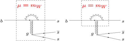
(a)                                   (b)

Figure 1: (a)$O_{3}-O_{6}$ contributions which include $(\delta_{LL,RR})_{23}$ mass insertions. (b) $O_{g}$ contribution which includes $(\delta_{LL,RR,LR,RL})_{23}$ mass insertions.

As emphasised in [7], the leading contribution to $\Delta B=1$ processes come from the chromomagnetic penguin operator $O_{g}(\tilde{O}_{g})$, in particular from the part proportional to the LR (RL) mass insertions which is enhanced by a factor $m_{\tilde{g}}/m_{b}$, where $C_{g}$ $\tilde{C}_{g}$ are given by

$$C_{g}\sim\frac{\alpha_{s}\pi}{\tilde{m}}\frac{m_{\tilde{g}}}{m_{b}}(\delta^{d}_{23})_{LR}\ \ \ \ \ \tilde{C}_{g}\sim\frac{\alpha_{s}\pi}{\tilde{m}}\frac{m_{\tilde{g}}}{m_{b}}(\delta^{d}_{23})_{RL}.$$ (7)

Note that the mass insertions appearing in the box diagrams are $(\delta_{AB})_{13}$ ($A,B=L\ \mbox{or}\ R$), thus, SUSY contributions to box diagram and to penguin diagram are independent. $S_{J/\psi}\simeq\sin 2\beta$ indicates the smallness of $(\delta_{AB})_{13}$ [8].

3 Can we explain the experimental data of $S_{\phi K_{S}}$ in SUSY?

Following the parametrisation of the SM and SUSY amplitudes in Ref.[7], $S_{\phi K_{S}}$ can be written as

$$S_{\phi K_{S}}=\frac{\displaystyle{\sin 2\beta+2R_{\phi}\cos\delta_{12}\sin(\theta_{\phi}+2\beta)+R_{\phi}^{2}\sin(2\theta_{\phi}+2\beta)}}{\displaystyle{1+2R_{\phi}\cos\delta_{12}\cos\theta_{\phi}+R_{\phi}^{2}}}$$ (8)

where $R_{\phi}=|A^{\mbox{\tiny SUSY}}/A^{\mbox{\tiny SM}}|$, $\theta_{\phi}=\mathrm{arg}(A^{\mbox{\tiny SUSY}}/A^{\mbox{\tiny SM}})$, and $\delta_{12}$ is the strong phase.

We will discuss in the following whether the SUSY contributions can make $S_{\phi K_{S}}$ negative. Note that the mass insertions $(\delta_{AB})_{23}$ have already been constrained by the experimental data for $Br(B\to X_{s}\gamma)$ :

$$|(\delta_{LL,RR})_{23}|\leq 1,\ \ \ \ \ \ |(\delta_{LR,RL})_{23}|\leq 1.6\times 10^{-2}$$ (9)

For $m_{\tilde{q}}=m_{\tilde{g}}=500$ GeV, we obtain

$$\frac{A^{\mathrm{SUSY}}}{A^{\mathrm{SM}}}=0.23(\delta_{LL})_{23}+0.23(\delta_{RR})_{23}+97.4(\delta_{LR})_{23}+97.4(\delta_{RL})_{23}$$ (10)

The constrains from $Br(B\to X_{s}\gamma)$ gives the maximum $|A^{\mathrm{SUSY}}|/|A^{\mathrm{SM}}|$:

$$\frac{|A^{\mathrm{SUSY}}|}{|A^{\mathrm{SM}}|} < 0.23\ \ \ \ \ \mbox{For}\ \ (\delta_{LL,RR})_{23}$$ (11)

$$\frac{|A^{\mathrm{SUSY}}|}{|A^{\mathrm{SM}}|} < 1.6\ \ \ \ \ \mbox{For}\ \ (\delta_{LR,RL})_{23}$$ (12)

In Fig.2, we present plots for the phase of $(\delta_{LL(RR)}^{d})_{23}$ and $(\delta_{LR(RL)}^{d})_{23}$ versus the mixing CP asymmetry $S_{\phi K_{S}}$ when the strong phases are ignored. We choose the three values of the magnitude of these mass insertions within the bounds from the experimental limits from $B\to X_{s}\gamma$. Each plot shows a contribution from an individual mass insertion by setting the other three to be zero. As can be seen from these plots, the $LR$ (same for $RL$) gives the largest contribution to $S_{\phi K_{S}}$. In order to have a sizable effect from the $LL$ or $RR$, the magnitude of $(\delta_{LL(RR)}^{d})_{23}$ has to be of order one and furthermore, the imaginary part needs to be as large as the real part. In any case, it is very difficult to give negative value of $S_{\phi K_{S}}$ from $(\delta_{LL}^{d})_{23}$ or $(\delta_{RR}^{d})_{23}$ mass insertion. If the experimental data remains as small as the current values, $LL,RR$ dominated models would get sever constrains on some parameters. Note that $S_{\phi K_{S}}$ decreases as SUSY masses becomes smaller. In [9], a choice of $m_{\tilde{q}}\simeq 350$ GeV has been used and a negative $S_{\phi K_{S}}$ for $LL,RR$ models has been obtained.

\psfrag{(a)}[l][l][0.8]{(a)\ \ $|(\delta_{LL(RR)}^{d})_{23}|$}\psfrag{(c)}[l][l][0.8]{(b)\ \ $|(\delta_{LR(RL)}^{d})_{23}|$}\psfrag{s}[r][l][0.8]{$S_{\phi K_{S}}$}\psfrag{1ll}[l][l][0.5]{\Large$0.1$}\psfrag{2ll}[l][l][0.5]{\Large$0.5$}\psfrag{3ll}[l][l][0.5]{\Large$\ \ 1$}\psfrag{1lr}[l][l][0.5]{\Large$0.001$}\psfrag{2lr}[l][l][0.5]{\Large$0.005$}\psfrag{3lr}[l][l][0.5]{\Large$0.01$}\psfrag{ll}[l][l][0.6]{$\arg[(\delta_{LL(RR)}^{d})_{23}]$}\psfrag{lr}[l][l][0.6]{$\arg[(\delta_{LR(RL)}^{d})_{23}]$}\includegraphics[width=227.62204pt]{figure2.eps}

Figure 2: Result for $S_{\phi K_{S}}$ in terms of the phase in mass insertions.

4 What happened to the $B\to\eta^{\prime}K_{S}$ process?

Although $B\to\phi K_{S}$ and $B\to\eta^{\prime}K_{S}$ are very similar processes, the parity of the final states can deviate the result. In the naive factorisation approximation, the amplitudes are written as a product of Wilson coefficients, form factors and decay constants:

$$A(B\to\phi(\eta^{\prime})K)\propto C_{\mbox{\tiny Wilson}}\ F^{B\to K}f_{\phi(\eta^{\prime})}$$ (13)

The decay constants appear in the calculation by sandwiching the $V\pm A$ current ($O_{i}$ and $\tilde{O}_{i}$ contributions, respectively) with $\phi(\eta^{\prime})$ and vacuum:

$$\langle 0|\overline{s}\gamma_{\mu}(1\pm\gamma_{5})s|\phi\rangle = m_{\phi}f_{\phi}\epsilon_{\mu}$$ (14)

$$\langle 0|\overline{s}\gamma_{\mu}(1\pm\gamma_{5})s|\eta^{\prime}\rangle = \pm if_{\eta^{\prime}}p_{\mu}$$ (15)

As can be seen from Eqs. (14) and (15), the vector meson $\phi$ picks up the $\gamma_{\mu}$ term while the pseudoscalar meson $\eta^{\prime}$ picks up the $\gamma_{\mu}\gamma_{5}$ term so that contributions from $O_{i}$ and $\tilde{O}_{i}$ obtain opposite signs for $\eta^{\prime}$.

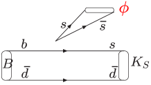
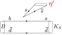
Figure 3: Schematically described naive factorisation approximation for $B\to\phi K_{S}$ and $B\to\eta^{\prime}K_{S}$ processes.

As a result, the sign of the $RR$ and $RL$ contributions are different for $B\to\phi K_{S}$ and $B\to\eta^{\prime}K_{S}$ [10]:

$$\!\!\left(\frac{A^{\mathrm{SUSY}}}{A^{\mathrm{SM}}}\right)_{\phi K_{S}}\!\!\!\!\! \!=\!\!\! \!0.23(\delta_{LL})_{23}\!+\!0.23(\delta_{RR})_{23}\!+\!97.4(\delta_{LR})_{23}\!+\!97.4(\delta_{RL})_{23}$$

$$\!\!\left(\frac{A^{\mathrm{SUSY}}}{A^{\mathrm{SM}}}\right)_{\eta^{\prime}K_{S}}\!\!\!\! \!=\!\!\! \!0.23(\delta_{LL})_{23}\!-\!0.23(\delta_{RR})_{23}\!+\!101(\delta_{LR})_{23}\!-\!101(\delta_{RL})_{23}$$

Since the coefficient for each mass insertions are similar, we use the following definition to simplify our following discussions:

$$\left(\frac{A^{\mathrm{SUSY}}}{A^{\mathrm{SM}}}\right)_{\phi K_{S}}\equiv\delta_{L}+\delta_{R}\ \ \ \ \left(\frac{A^{\mathrm{SUSY}}}{A^{\mathrm{SM}}}\right)_{\eta^{\prime}K_{S}}\equiv\delta_{L}-\delta_{R}$$ (16)

where $\delta_{L}$ includes contributions from $(\delta_{LL})_{23}$ and $(\delta_{LR})_{23}$ and $\delta_{R}$ includes contributions from $(\delta_{RR})_{23}$ and $(\delta_{RL})_{23}$. Now let us show how this sign flip effects to the mixing CP violation $S_{\phi KS}$ and $S_{\eta^{\prime}K_{S}}$. Since both $\delta_{L}$ and $\delta_{R}$ are complex number, we have four parameters to be fixed while we have only two experimental data. Thus, we fix two parameters and perform a case-by-case study in the following.

• Case 1: $|\delta_{R}|\gg|\delta_{L}|$

  $$\left(\frac{A^{\mathrm{SUSY}}}{A^{\mathrm{SM}}}\right)_{\phi K_{S}} = |\delta_{R}|e^{i\arg\delta_{R}},$$

  $$\left(\frac{A^{\mathrm{SUSY}}}{A^{\mathrm{SM}}}\right)_{\eta^{\prime}K_{S}} = |\delta_{R}|e^{i(\arg\delta_{R}+\pi)}.$$

• Case 2: $|\delta_{L}|=|\delta_{R}|$ ($\Delta\theta=\arg\delta_{L}-\arg\delta_{R}$)

  $$\left(\frac{A^{\mathrm{SUSY}}}{A^{\mathrm{SM}}}\right)_{\phi K_{S}} = 2|\delta_{L}|\cos\frac{\Delta\theta}{2}e^{i(\arg\delta_{L}+\arg\delta_{R})/2}$$

  $$\left(\frac{A^{\mathrm{SUSY}}}{A^{\mathrm{SM}}}\right)_{\eta^{\prime}K_{S}} = 2|\delta_{L}|\sin\frac{\Delta\theta}{2}e^{i(\arg\delta_{L}+\arg\delta_{R}+\pi)/2}$$

• Case 3: $\arg\delta_{L}=\arg\delta_{R}$ ($\Delta|\delta|=|\delta_{L}|-|\delta_{R}|$)
  

  $$\left(\frac{A^{\mathrm{SUSY}}}{A^{\mathrm{SM}}}\right)_{\phi K_{S}} = (|\delta_{L}|+|\delta_{R}|)e^{i\arg\delta_{L}}$$

  $$\left(\frac{A^{\mathrm{SUSY}}}{A^{\mathrm{SM}}}\right)_{\eta^{\prime}K_{S}} = \Delta|\delta|e^{i\arg\delta_{L}}$$

• Case 4: $\arg\delta_{R}=\arg\delta_{L}+\pi/2$ ($\tan\alpha=|\delta_{R}|/|\delta_{L}|$)
  

  $$\left(\frac{A^{\mathrm{SUSY}}}{A^{\mathrm{SM}}}\right)_{\phi K_{S}} = \sqrt{|\delta_{L}|^{2}+|\delta_{R}|^{2}}e^{i(\arg\delta_{L}+\alpha)}$$

  $$\left(\frac{A^{\mathrm{SUSY}}}{A^{\mathrm{SM}}}\right)_{\eta^{\prime}K_{S}} = \sqrt{|\delta_{L}|^{2}+|\delta_{R}|^{2}}e^{i(\arg\delta_{L}-\alpha)}$$

In Fig. 4, we show some examples of the parameter sets with which we can reproduce both experimental data of $S_{\phi K_{S}}$ and $S_{\eta^{\prime}K_{S}}$.

\psfrag{phi}[l][l]{$S_{\phi K_{S}}^{\mbox{\tiny exp.}}$}\psfrag{eta}[l][l]{$S_{\eta^{\prime}K_{S}}^{\mbox{\tiny exp.}}$}\psfrag{s}[l][l]{$S_{\phi K_{S},\eta^{\prime}K_{S}}$}\psfrag{t}[l][l]{$\theta_{\phi K_{S}}$}\includegraphics[width=227.62204pt]{fig1.eps}

Figure 4: Case 1: $|\delta_{R}|$ dominating. Case 2: $|\delta_{R}|=|\delta_{L}|$ with $\Delta\theta=\pi/10$. Case 3: $\arg\delta_{L}=\arg\delta_{R}$ with $\Delta|\delta|=+0.2$. Case 4: $\arg\delta_{R}=\arg\delta_{L}+\pi/2$ with $\alpha=3\pi/8$. Solid line: $S_{\phi K_{S}}$ for $|A^{\mathrm{SUSY}}|/|A^{\mathrm{SM}}|=0.5$.

5 On the branching ratio of $B\to\eta^{\prime}K_{S}$: Gluonium vs. New physics

In 1997, CLEO collaboration reported an unexpectedly large branching ratio [11]

$$Br^{\mbox{\tiny exp.}}(B^{0}\to K^{0}\eta^{\prime})=(89^{+18}_{-16}\pm 9)\times 10^{-6}$$ (17)

which is confirmed by Belle [12] and BABAR [4]:

BELLE $$= (79^{+12}_{-16}\pm 8)\times 10^{-6},$$ (18)

BABAR $$= (76.9\pm 3.5\pm 4.4)\times 10^{-6}$$ (19)

Considering the theoretical prediction by the naive factorisation approximation

$$Br^{\mbox{\tiny theo.}}(B\to K\eta^{\prime})\simeq 25\times 10^{-6},$$ (20)

the experimental data is about factor of three large, thus, there have been various efforts to explain this puzzle. On one hand, new physics contributions have been discussed [13]. However, the enhancement by new physics contributions through penguin diagrams ends up with large branching ratios for all other penguin dominated processes. Therefore, one needs a careful treatment to enhance only $B\to\eta^{\prime}K$ process without changing the predictions for the other processes. On the other hand, since this kind of large branching ratio is observed only in $B\to\eta^{\prime}K$ process, the gluonium contributors which only exist in this process have been a very interesting candidate to solve the puzzle [14] [15] though the amount of gluonium in $\eta^{\prime}$ is not precisely known [16]. In this section, let us discuss the effect of our including SUSY contributions to the branching ratios for $B\to\phi K$ and $B\to\eta^{\prime}K$.

Inclusion of the SUSY contributions modify the branching ratio as:

$$Br^{\mbox{\tiny SM + SUSY}}=Br^{\mbox{\tiny SM}}\times[1+2\cos\theta_{\mbox{\tiny SUSY}}R+R^{2}]$$

where $R=|A^{\mathrm{SUSY}}|/|A^{\mathrm{SM}}|$. As we have shown, to achieve a negative value of $S_{\phi K_{S}}$, we need $\theta_{\mbox{\tiny SUSY}}\simeq-\pi/2$, which suppresses the leading SUSY contribution. As a result, for instance, $R=0.5$ leads to:

$$Br(B\to\phi K_{S})=(7.8\times 10^{-6})\times 1.25=9.7\times 10^{-6}$$ (21)

which is within the experimental data $(9.1\pm 2.6)\times 10^{-6}$. On the other hand, the phase for $B\to\eta^{\prime}K$ is different from the one for $\phi K_{S}$, as is discussed in the previous section. For instance, Case 2 gives us the maximum value of:

$$Br(B\to\eta^{\prime}K_{S})=(25\times 10^{-6})\times 3.25=81\times 10^{-6}$$ (22)

However, this kind of enhancement would appear all the other two pseudo-scalars channels (such as $B\to K\pi$) and might cause some problems.

As a whole, we would like to suggest that the solution for the branching ratio puzzle is not only the SUSY contribution but a combination of SUSY contribution and the gluonium contribution. Here, let us show the dependence of the gluonium contribution to the $S_{\eta^{\prime}K_{S}}$. Including the gluonium contribution (see Fig. 5), the amplitude is modified to

$$A=A^{\mbox{\tiny SM}}_{\eta^{\prime}K_{S}}+A^{\mbox{\tiny SUSY}}_{\eta^{\prime}K_{S}}+G^{\mbox{\tiny SM}}+G^{\mbox{\tiny SUSY}}$$ (23)

where $G^{\mbox{\tiny SM}}$ and $G^{\mbox{\tiny SUSY}}$ are the new mechanism contributions to SM and SUSY, respectively. Let us parametrise the unknown gluonium content in $\eta^{\prime}$ as $r=G^{\mbox{\tiny SM}}/A^{\mbox{\tiny SM}}_{\eta^{\prime}K_{s}}$. Our result is shown in Fig. 6 when we vary $r$ from 0 to 0.3. As can be seen from this figure, the dependence of $S_{\eta^{\prime}K_{s}}$ on $r$ is not very strong, therefore, we can enhance the branching ratio by gluonium contribution without disturbing our findings for $S_{\eta^{\prime}K_{S}}$ in the previous section.

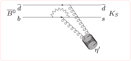
Figure 5: A contribution from gluonium content in $\eta^{\prime}$ to the $B\to\eta^{\prime}K$ process.

\psfrag{S}[l][l][1.2]{$S_{\eta^{\prime}K_{S}}$}\psfrag{B}[l][l][1.1]{$Br(B\to\eta^{\prime}K)/Br^{\mbox{\tiny SM}}(B\to\eta^{\prime}K)$}\psfrag{r}[l][l]{$r=0\rightarrow 0.3$}\psfrag{alpha}[l][l][0.7]{$\arctan|\delta_{R}|/|\delta_{L}|=\pi/2\rightarrow\pi/4$}\psfrag{dt}[l][r][0.7]{$(arg\delta_{L}-arg\delta_{R})=\pi/2\rightarrow\pi/10$}\psfrag{dd3}[l][l][0.7]{$|\delta_{L}|-|\delta_{R}|=-0.5\rightarrow+0.2$}\psfrag{c1}[l][l][1]{Case 1}\psfrag{c2}[l][l][1]{Case 2}\psfrag{c3}[l][l][1]{Case 3}\psfrag{c4}[l][l][1]{Case 4}\psfrag{sexp}[l][l][1.2]{$S_{\eta^{\prime}K_{S}}^{\mbox{\tiny exp}}$}\includegraphics[width=227.62204pt]{eta-fig2.eps}

Figure 6: Branching ratio versus the mixing CP asymmetry in the $B\to\eta^{\prime}K$ process. The parameter $r$ represents the contribution from the gluonium diagram.

6 Conclusions

We studied the supersymmetric contributions to the CP asymmetry of $B\to\phi K_{S}$ and $B\to\eta^{\prime}K_{S}$ in a model independent way. We found that the observed large discrepancy between $S_{J/\psi K_{S}}$ and $S_{\phi K_{S}}$ can be explained within some SUSY models with large $(\delta_{LR})_{23}$ or $(\delta_{RL})_{23}$ mass insertions. We showed that the SUSY contributions of $(\delta_{RR})_{23}$ and $(\delta_{RL})_{23}$ to $B\to\phi K_{S}$ and $B\to\eta^{\prime}K_{S}$ have different signs. Therefore, the current observation, $S_{\phi K_{S}}<S_{\eta^{\prime}K_{S}}$, favours the $(\delta_{RR,RL})_{23}$ dominated models. We also discussed the SUSY contributions to the branching ratios. We showed that negative $S_{\phi K_{S}}$ and small SUSY effect to $Br(B\to\phi K)$ can be simultaneously achieved. On the other hand, we showed that SUSY contribution itself does not solve the puzzle of the large branching ratio of $B\to\eta^{\prime}K_{S}$. We included the gluonium contributions to $B\to\eta^{\prime}K_{S}$. We found that our conclusion for $S_{\eta^{\prime}K_{S}}$does not disturbed by gluonium contributions. As soon as the experimental errors are reduced, the CP violation of $B\to\phi K_{S}$ and $B\to\eta^{\prime}K_{S}$ will be able to give a strong constraints on the $(\delta_{AB})_{23}$ mass insertions.

References

• [1] S.Β Abel, S.Β Khalil and O.Β Lebedev, Nucl.Β Phys.Β B 606, 151 (2001).
• [2] K.Β Abe et al. [Belle Collaboration], arXiv:hep-ex/0207098.
• [3] B.Β Aubert et al. [BABAR Collaboration], arXiv:hep-ex/0207070.
• [4] B.Β Aubert et al. [BABAR Collaboration], arXiv:hep-ex/0303046.
• [5] Y.Β Nir, Nucl.Β Phys.Β Proc.Β Suppl.Β  117 (2003) 111 [arXiv:hep-ph/0208080].
• [6] L.Β J.Β Hall, V.Β A.Β Kostelecky and S.Β Raby, Nucl.Β Phys.Β B 267 (1986) 415.
• [7] S.Β Khalil and E.Β Kou, Phys.Β Rev.Β D 67 (2003) 055009 [arXiv:hep-ph/0212023].
• [8] E.Β Gabrielli and S.Β Khalil, Phys.Β Rev.Β D 67, 015008 (2003) [arXiv:hep-ph/0207288].
• [9] M.Β Ciuchini, E.Β Franco, A.Β Masiero and L.Β Silvestrini, Phys.Β Rev.Β D 67 (2003) 075016 [arXiv:hep-ph/0212397].
• [10] S.Β Khalil and E.Β Kou, arXiv:hep-ph/0303214.
• [11] S.Β J.Β Richichi et al. [CLEO Collaboration], arXiv:hep-ex/9908019.
• [12] K.Β Abe et al. [Belle Collaboration], Phys.Β Lett.Β B 517, 309 (2001) [arXiv:hep-ex/0108010].
• [13] A.Β Kundu, Pramana 60 (2003) 345 [arXiv:hep-ph/0205100].
• [14] D.Β Atwood and A.Β Soni, Phys.Β Lett.Β B 405 (1997) 150 [arXiv:hep-ph/9704357].
• [15] M.Β R.Β Ahmady, E.Β Kou and A.Β Sugamoto, Phys.Β Rev.Β D 58 (1998) 014015 [arXiv:hep-ph/9710509].
• [16] E.Β Kou, Phys.Β Rev.Β D 63 (2001) 054027 [arXiv:hep-ph/9908214].