Abstract

We reanalyse the potential of the LHC to discover new $Z^{\prime}$ gauge bosons and to discriminate between various theoretical models. Using a fast LHC detector simulation, we have investigated how well the characteristics of $Z^{\prime}$ bosons from different models can be measured. For this analysis we have combined the information coming from the cross section measurement, which provides also the $Z^{\prime}$ mass and total width, the forward-backward charge asymmetries on- and off-peak, and the $Z^{\prime}$ rapidity distribution, which is sensitive to its $u\bar{u}$ and $d\bar{d}$ couplings. We confirm that new $Z^{\prime}$ bosons can be observed in the process $pp\to Z^{\prime}\to\ell^{+}\ell^{-}$, up to masses of about 5 TeV for an integrated luminosity of 100 fb^-1. The off- and on-resonance peak forward-backward charge asymmetries $A_{\rm FB}^{\ell}$ show that interesting statistical accuracies can be obtained up to $Z^{\prime}$ masses of the order of 2 TeV. We then show how the different experimental observables allow for a diagnosis of the $Z^{\prime}$ boson and the distinction between the various considered models.

1. Introduction

Although the Standard Model (SM) of the electroweak and strong interactions describes nearly all experimental data available today [1], it is widely believed that it is not the ultimate theory. Grand Unified Theories (GUTs), eventually supplemented by Supersymmetry to achieve a successful unification of the three gauge coupling constants at the high scale, are prime candidates for the physics beyond the SM. Many of these GUTs, including superstring and left-right-symmetric models, predict the existence of new neutral gauge bosons, which might be light enough to be accessible at current and/or future colliders; for reviews see Ref. [3]. New vector bosons also appear in models of dynamical symmetry breaking [4] and recently, “little Higgs” models have been proposed to solve the hierarchy problem of the SM [5]: they have large gauge group structures and therefore predict a plethora of new gauge bosons with masses in the TeV range.

The search for these $Z^{\prime}$ particles is an important aspect of the experimental physics program of future high-energy colliders. Present limits from direct production at the Tevatron and virtual effects at LEP, through interference or mixing with the $Z$ boson, imply that new $Z^{\prime}$ bosons are rather heavy and mix very little with the $Z$ boson. Depending on the considered theoretical models, $Z^{\prime}$ masses of the order of 500 to 800 GeV and $Z$–$Z^{\prime}$ mixing angles at the level of a few per-mile are excluded [7]. A $Z^{\prime}$ boson, if lighter than about 1 TeV, could be discovered at Run II of the Tevatron [8] in the Drell-Yan process $p\bar{p}\to Z^{\prime}\to\ell^{+}\ell^{-}$, with $\ell=e,\mu$ [9]. Detailed theoretical [8] and experimental [10, 11, 12] analyses have shown that the discovery potential of the LHC experiments is about 5 TeV, using the process $pp\to Z^{\prime}\to\ell^{+}\ell^{-}$. Future $e^{+}e^{-}$ colliders with high c.m. energies and longitudinally polarized beams could indicate the existence of $Z^{\prime}$ bosons via its interference effects, with masses up to about $6\times\sqrt{s}$ [8, 13].

After the discovery of a $Z^{\prime}$ boson, some diagnosis of its coupling needs to be done in order to identify the correct theoretical frame. For this purpose, and since a long time, the forward-backward charge asymmetry for leptons $A_{\rm FB}^{\ell}$ has been advocated as being a powerful tool [14]; the most direct method to actually measure $A_{\rm FB}^{\ell}$ at the LHC has been described in [15]. In addition to the information from the total $Z^{\prime}$ cross section, it has been argued that the measurement of ratios of $Z^{\prime}$ cross sections in different rapidity bins might provide some information about the $Z^{\prime}$ couplings to up and down quarks [16].

Following the arguments given in [17], we advocate that the $Z^{\prime}$ cross section should be measured relative to the number of produced $Z$ bosons for the same lepton final states. Using this approach, many systematic uncertainties due to theoretical and experimental uncertainties will cancel, and the relative $Z^{\prime}/Z$ cross section ratio might be measured and calculated with an accuracy of about 1%. Furthermore, the method should also lead to precise relative parton distribution functions for $u$ and $d$ quarks, as well as for the corresponding sea quarks and antiquarks. Thus, we can go beyond the previously proposed procedure to analyse the $Z^{\prime}$ rapidity distribution [16], by performing a fit. The fit uses the predicted rapidity spectra as calculated with $u\bar{u}$ and $d\bar{d}$, as well as the contribution of the sea, for the mass region of interest, which is directly related to $x_{1},x_{2}$ of the corresponding quarks and antiquarks in the proton.

While numerous theoretical and experimentally motivated $Z^{\prime}$ studies have already been performed, the combination of all sensitive LHC variables, as described above, has not been done so far; the work described in this paper will thus fill a gap. We will perform the studies using the PYTHIA program [18] and a fast LHC detector simulation. We first update previous studies using, the latest parton distribution functions [21], and extend them in two directions. First, following the method proposed in [15], the forward-backward charge asymmetries, on and off the $Z^{\prime}$ resonance peak, are analysed together with the cross section in order to differentiate between the different models. Second, we show that a direct fit of the rapidity distribution allows for additional information and would be useful to disentangle between $Z^{\prime}$ bosons from various models through their different couplings to up-type and down-type quarks.

The rest of the discussion will be organized as follows. In the next section, we define the theoretical framework in which our analysis will be performed. In section 3, we describe the relevant observables that can be measured at the LHC, namely the dilepton cross section times the $Z^{\prime}$ total width, the on-peak and off-peak forward-backward asymmetries and the rapidity distribution, and the simulation tools which we will use in our study. In section 4, we analyse the resolving power of these observables.

2. The considered $Z^{\prime}$ models

To simplify the discussion, we will focus in this paper on two effective theories of well motivated models that lead to an extra gauge boson:

1) An effective ${\rm SU(2)_{L}\times U(1)_{Y}\times U(1)_{Y^{\prime}}}$ model, which originates from the breaking of the exceptional group E₆, which is general enough to include many interesting possibilities. Indeed, in the breaking of this group down to the SM symmetry, two additional neutral gauge bosons could appear. For simplicity we assume that only the lightest $Z^{\prime}$ can be produced at the LHC. It is defined as

$$Z^{\prime}=Z^{\prime}_{\chi}\cos\beta+Z^{\prime}_{\psi}\sin\beta$$ (1)

and can be parametrized in terms of the hypercharges of the two groups U(1)_ψ and U(1)_χ which are involved in the breaking chain:

${\rm E_{6}\to SO(10)\times U(1)_{\psi}\to SU(5)\times U(1)_{\chi}\times U(1)_{\psi}\to SU(3)_{c}\times SU(2)_{L}\times U(1)_{Y}\times U(1)_{Y^{\prime}}}$

The values $\beta=0$ and $\beta=\pi/2$ would correspond, respectively, to pure $Z^{\prime}_{\chi}$ and $Z^{\prime}_{\psi}$ bosons, while the value $\beta={\rm arctan}(-\sqrt{5/3})$ would correspond to a $Z^{\prime}_{\eta}$ boson originating from the direct breaking of ${\rm E_{6}}$ to a rank-5 group in superstrings inspired models.

2) Left-right (LR) models, based on the symmetry group ${\rm SU(2)_{R}\times SU(2)_{L}\times U(1)_{B-L}}$, where $B$ and $L$ are the baryon and lepton numbers. Even though we investigate only the $Z^{\prime}$ in this paper, it should be recalled that new charged vector bosons, potentially observable at the LHC, also appear in these models. The most general neutral boson $Z^{\prime}_{LR}$ will couple to a linear combination of the right-handed and $B$–$L$ currents:

$$J_{LR}^{\mu}=\alpha_{LR}J^{\mu}_{3R}-(1/2\alpha_{LR})J^{\mu}_{B-L}\ \ {\rm with}\ \alpha_{LR}=\sqrt{(c_{W}^{2}g_{R}^{2}/s_{W}^{2}g_{L}^{2})-1}\ ,$$ (2)

where $g_{L}$=$e/s_{W}$ and $g_{R}$ are the ${\rm SU(2)_{L}}$ and ${\rm SU(2)_{R}}$ coupling constants with $s_{W}^{2}=1-c_{W}^{2}\equiv\sin^{2}\theta_{W}$. The parameter $\alpha_{LR}$ is restricted to lie in the range $\sqrt{2/3}\raisebox{-3.69899pt}{~{}\shortstack{$<$ \\ [-0.07cm] $\sim$}}~{}\alpha_{LR}\raisebox{-3.69899pt}{~{}\shortstack{$<$ \\ [-0.07cm] $\sim$}}~{}\sqrt{2}$: the upper bound corresponds to a LR-symmetric model with $g_{R}=g_{L}$, abbreviated in the following as $LR$, while the lower bound corresponds to the $\chi$ model discussed in scenario (1), since SO(10) can lead to both ${\rm SU(5)\times U(1)}$ and ${\rm SU(2)_{R}\times SU(2)_{L}\times U(1)}$ breaking patterns.

In order to achieve a complete comparison, we will also discuss the non-realistic case of a sequential boson $Z^{\prime}_{\rm SM}$, which has the same fermion couplings as the SM $Z$ boson, as well as a $Z^{\prime}$ boson, denoted by $Z^{\prime}_{d}$, with vanishing axial and vectorial couplings to $u$ quarks and which, in $E_{6}$ models, corresponds to the choice $\cos\beta=\sqrt{5/8}$.

The left- and right-handed couplings of the $Z^{\prime}$ boson to fermions, defined as:

$$g_{Z^{\prime}}J^{\mu}_{Z^{\prime}}Z^{\prime}_{\mu}=\frac{e}{c_{W}}\sum_{f}\gamma^{\mu}\left[\frac{1-\gamma_{5}}{2}\,g_{L}^{fZ^{\prime}}+\frac{1+\gamma_{5}}{2}\,g_{R}^{fZ^{\prime}}\right]\ ,$$ (3)

are given in Table 1 for the first-generation fermions in the two scenarios. The mixing between the $Z$ and $Z^{\prime}$ bosons is very small [7] and will be neglected in our discussion.

$f$	$g_{L}^{fZ^{\prime}}|_{E_{6}}$	$g_{R}^{fZ^{\prime}}|_{E_{6}}$	$g_{L}^{fZ^{\prime}}|_{LR}$	$g_{R}^{fZ^{\prime}}|_{LR}$
$\nu_{e}$	$\frac{3\cos\beta}{2\sqrt{6}}+\frac{\sqrt{10}\sin\beta}{12}$	$0$	$\frac{1}{2\alpha_{LR}}$	$0$
$e$	$\frac{3\cos\beta}{2\sqrt{6}}+\frac{\sqrt{10}\sin\beta}{12}$	$\frac{\cos\beta}{2\sqrt{6}}-\frac{\sqrt{10}\sin\beta}{12}$	$\frac{1}{2\alpha_{LR}}$	$\frac{1}{2\alpha_{LR}}-\frac{\alpha_{LR}}{2}$
$u$	$-\frac{\cos\beta}{2\sqrt{6}}+\frac{\sqrt{10}\sin\beta}{12}$	$\frac{\cos\beta}{2\sqrt{6}}-\frac{\sqrt{10}\sin\beta}{12}$	$-\frac{1}{6\alpha_{LR}}$	$-\frac{1}{6\alpha_{LR}}+\frac{\alpha_{LR}}{2}$
$d$	$-\frac{\cos\beta}{2\sqrt{6}}+\frac{\sqrt{10}\sin\beta}{12}$	$-\frac{3\cos\beta}{2\sqrt{6}}-\frac{\sqrt{10}\sin\beta}{12}$	$-\frac{1}{6\alpha_{LR}}$	$-\frac{1}{6\alpha_{LR}}-\frac{\alpha_{LR}}{2}$

Table 1: Left- and right-handed couplings of the $Z^{\prime}$ boson to the SM fermions with the notation of the first generation in the $E_{6}$ (left panels) and LR (right panels) models.

The $Z^{\prime}$ partial decay width into a massless fermion-antifermion pair reads

$$\Gamma_{Z^{\prime}}^{f}=N_{c}\frac{\alpha M_{Z^{\prime}}}{6c_{W}^{2}}\left[(g_{L}^{fZ^{\prime}})^{2}+(g_{R}^{fZ^{\prime}})^{2}\right]$$ (4)

with $N_{c}$ the colour factor and the electromagnetic coupling constant to be evaluated at the scale $M_{Z^{\prime}}$ leading to $\alpha\sim 1/128$. In the absence of any exotic decay channel, the branching fractions for decays into the first-generation leptons and quarks are shown in Fig. 1 for $E_{6}$ and LR models as functions of $\cos\beta$ and $\alpha_{LR}$, respectively. As can be seen, the decay fractions into $\ell^{+}\ell^{-}$ pairs are rather small, varying between 6.6% and 3.4% for $E_{6}$ models and 6.6% and 2.3% for LR models; in the latter case the decay branching fraction is largest for the symmetric case $g_{L}=g_{R}$ and smallest for $\alpha_{LR}\simeq\sqrt{2}$. The $Z^{\prime}$ total decay width, normalized to $M_{Z^{\prime}}$, is also shown in Fig. 1: it is largest when $\cos\beta=\pm 1$ in $E_{6}$ models and $\alpha_{LR}\simeq\sqrt{2}$ in LR ones. The $Z^{\prime}$ bosons that we will consider here are thus narrow resonances, since their total decay width does not exceed 2% of their masses.

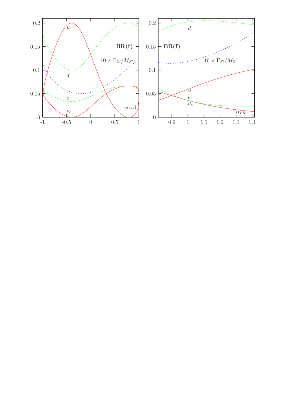
Figure 1: The branching ratios of the decays $Z^{\prime}\to f\bar{f}$ in $E_{6}$ models as a function of $\cos\beta$ (left) and in LR models as a function of $\alpha_{LR}$ (right). The total $Z^{\prime}$ decay widths, normalized to $10/M_{Z^{\prime}}$, are also shown.

In the limit of negligible fermion masses, the differential cross section for the subprocess $q\bar{q}\to\ell^{+}\ell^{-}$, with respect to $\theta^{*}$ defined as the angle between the initial quark $q$ and the final lepton $\ell^{-}$ in the $Z^{\prime}$ rest frame, is given by $[\hat{s}=M^{2}_{\ell\ell}$ is the c.m.  energy of the subprocess]

$$\frac{{\rm d}\hat{\sigma}}{{\rm d}\cos\theta^{*}}\,(q\bar{q}\to\gamma,Z,Z^{\prime}\to\ell^{+}\ell^{-})=\frac{1}{9}\frac{\pi\alpha^{2}}{2\hat{s}}\left[(1+\cos^{2}\theta^{*})Q_{1}+2\cos\theta^{*}Q_{3}\right]\ ,$$ (5)

where the charges $Q_{1}$ and $Q_{3}$ are given by [13]

$$Q_{1/3}=\left[\,|Q_{LL}|^{2}+|Q_{RR}|^{2}\pm|Q_{RL}|^{2}\pm|Q_{LR}|^{2}\,\right]/4\ .$$ (6)

In terms of the left- and right-handed couplings of the $Z^{\prime}$ boson defined previously, and of those of the $Z$ boson [$g_{L}^{fZ}=I_{3L}^{f}-Q^{f}s_{W}^{2},\,g_{R}^{fZ}=-Q_{f}s_{W}^{2}$] and the photon [$g_{L}^{f\gamma}=g_{R}^{f\gamma}=Q_{f}$] with $Q^{f}$ the electric charge and $I_{3L}^{f}$ the left-handed weak isospin, the helicity amplitudes $Q_{ij}$ with $i,j=L,R$ for a given initial $q\bar{q}$ state read

$$Q_{ij}^{q}=g_{i}^{q\gamma}g_{j}^{\ell\gamma}+\frac{g_{i}^{qZ}g_{j}^{\ell Z}}{s_{W}^{2}c_{W}^{2}}\frac{\hat{s}}{\hat{s}-M_{Z}^{2}+i\Gamma_{Z}M_{Z}}+\frac{g_{i}^{qZ^{\prime}}g_{j}^{\ell Z^{\prime}}}{c_{W}^{2}}\frac{\hat{s}}{\hat{s}-M_{Z^{\prime}}^{2}+i\Gamma_{Z^{\prime}}M_{Z^{\prime}}}\ .$$ (7)

To obtain the total hadronic cross section and forward-backward asymmetries, we must sum over the contributing quarks and fold with the parton luminosities.

A few points are worth recalling concerning the forward-backward asymmetry in $E_{6}$ models [14]: $(i)$ since the up-type quarks have no axial couplings to the $Z^{\prime}$ boson, $Q_{3}^{q}=0$, they do not contribute to $A_{\rm FB}^{\ell}$ on the $Z^{\prime}$ peak; $(ii)$ the asymmetry completely vanishes for three $\beta$ values: $\beta={\rm arctan}(-\sqrt{3/5})$ and $\beta=\pm\pi/2$, where the left- and right-handed $Z^{\prime}$ couplings of both $d$-quarks and charged leptons are equal; $(iii)$ off the $Z^{\prime}$ resonance, there is always an asymmetry that is generated by the $Z$ boson couplings.

3. Observables sensitive to $Z^{\prime}$ properties

The LHC discovery potential for a $Z^{\prime}$ as a mass peak above a small background in the reaction $pp\rightarrow Z^{\prime}\rightarrow\ell^{+}\ell^{-}$, with $\ell=e,\mu$, is well known. The required luminosity to discover a $Z^{\prime}$ basically depends only on its cross section, and therefore on its mass and couplings. Experimental effects due to mass resolution, assuming the design parameters of ATLAS or CMS [11, 12], are known to result in an only minor reduction of the sensitivity.

Once a $Z^{\prime}$ boson is observed at the LHC, we will obviously measure its mass, its total width and cross section. Furthermore, forward-backward charge asymmetries on and off the $Z^{\prime}$ resonance provide additional information about its couplings and interference effects with the $Z$ boson and the photon. In addition one can include the analysis of the $Z^{\prime}$ rapidity distribution, which is sensitive to the $Z^{\prime}$ couplings to $u\bar{u}$ and $d\bar{d}$ quarks. Such future measurements can be performed as follows at the LHC:

The total decay width of the $Z^{\prime}$ is obtained from a fit to the invariant mass distribution of the reconstructed dilepton system using a non-relativistic Breit-Wigner function: $a_{0}/[(M_{\ell\ell}^{2}-M_{Z^{\prime}}^{2})^{2}+a_{1}]$ with $a_{1}=\Gamma_{Z^{\prime}}^{2}M_{Z^{\prime}}^{2}$.

The $Z^{\prime}$ cross section times leptonic branching ratio is calculated from the number of reconstructed dilepton events lying within $\pm 3\Gamma$ around the observed peak. The $3\Gamma$ interval used to define the cross section is arbitrary; however, if varied from $2\Gamma$ to $5\Gamma$, the cross section increases only between 5 and 10% for different $Z^{\prime}$ models and masses.

The leptonic forward-backward charge asymmetry $A_{\rm FB}^{\ell}$ is defined from the lepton angular distribution with respect to the quark direction in the centre-of-mass frame, as:

$$\mathrm{\frac{d\sigma}{d\cos\theta^{*}}\propto\frac{3}{8}(1+\cos^{2}\theta^{*})+A_{\rm FB}^{\ell}\cos\theta^{*}}\ .$$ (8)

As discussed in Ref. [15], the lepton angle $\theta^{*}$ in the dilepton c.m.  frame can be calculated using the measured four momenta of the dilepton system. $A_{\rm FB}^{\ell}$ can then be determined with an unbinned maximum likelihood fit to the $\cos\theta^{*}$ distribution. Figure 2a shows the asymmetry, assuming that the quark direction is known, as a function of the dilepton mass for a $Z_{\chi}^{\prime}$ and a $Z_{\rm SM}^{\prime}$ boson, assuming a mass $M_{Z^{\prime}}=1.5$ TeV. $A_{\rm FB}^{\ell}$ varies strongly with the dilepton mass and is very different in the two models. Unfortunately, $A_{\rm FB}^{\ell}$ cannot be measured directly in a proton-proton collider, as the original quark direction is not known. However, it can be extracted from the kinematics of the dilepton system, as was shown in detail in [15]. The method is based on the different $x$ spectra of the quarks and antiquarks in the proton, which allows to approximate the quark direction with the boost direction of the $\ell\ell$ system with respect to the beam axis (the $z$ axis). Consequently, the probability to assign the correct quark direction increases for larger rapidities of the dilepton system and somewhat cleaner and more significant measurements can be performed, as shown in Fig. 2b. A purer, though smaller, signal sample can thus be obtained by introducing a rapidity cut. For the following studies we will require $|Y_{\ell\ell}|>0.8$.

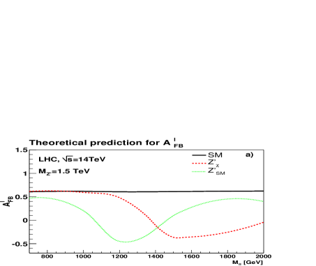
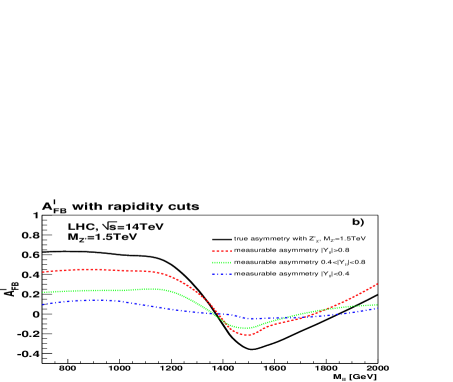
Figure 2: $A_{FB}^{\ell}$ as a function of the dilepton mass: the predicted asymmetry for a $Z^{\prime}_{\chi}$ and a $Z^{\prime}_{SM}$ together with the SM prediction (a) and in different dilepton intervals (b).

The $Z^{\prime}$ rapidity distribution allows us to obtain the fraction of $Z^{\prime}$ bosons produced from $u\bar{u}$ and $d\bar{d}$ initial states. Assuming that the $W^{\pm}$ and $Z$ boson rapidity distributions have been measured in detail, as discussed in [17], relative parton distribution functions for $u$ and $d$ quarks, as well as for the corresponding sea quarks and antiquarks are well known. Thus, the rapidity spectra can be calculated separately for $u\bar{u}$ and $d\bar{d}$, as well as for sea quark antiquark annihilation, and for the mass region of interest. Using these distributions, a fit can be performed to the $Z^{\prime}$ rapidity distribution, which allows to obtain the corresponding fractions of the $Z^{\prime}$ boson produced from $u\bar{u}$, $d\bar{d}$ as well as for sea quark-antiquark annihilation.

In the present analysis, PYTHIA events of the type $pp\to\gamma,Z,Z^{\prime}\to ee,\mu\mu$ were simulated at a centre-of-mass energy of 14 TeV, and for the $Z^{\prime}$ models discussed in section 2. The $Z^{\prime}$ masses were varied from 1 TeV up to 5 TeV. These events were analysed, using simple acceptance cuts following the design criteria of ATLAS and CMS. Following the results from previous studies and the expected excellent detector resolutions, the obtained values are known to be rather insensitive to measurement errors, especially for the $e^{+}e^{-}$ final states. We therefore do not include any resolution for the current study. In detail, the following basic event selection criteria were used:

• The transverse momenta of the leptons, $p_{T}^{\ell}$ , should be at least 20 GeV.

• The pseudorapidity $|\eta|$ of each lepton should be smaller than 2.5.

• The leptons should be isolated, requiring that the lepton carries at least 95% of the total transverse energy found in a cone of size of 0.5 around the lepton.

• There should be exactly two isolated leptons with opposite charge in each event.

• The two leptons should be back to back in the plane transverse to the beam direction, so that the opening angle between them was larger than $160^{\circ}$.

Figure 3 shows the expected number of events for a luminosity of 100 fb^-1. The SM background relative to the signal cross section is found to be essentially negligible for the considered $Z^{\prime}$ models. We thus reconfirm the known $Z^{\prime}$ boson LHC discovery potential, to reach masses up to about 5 TeV for a luminosity of 100 fb^-1 [8].

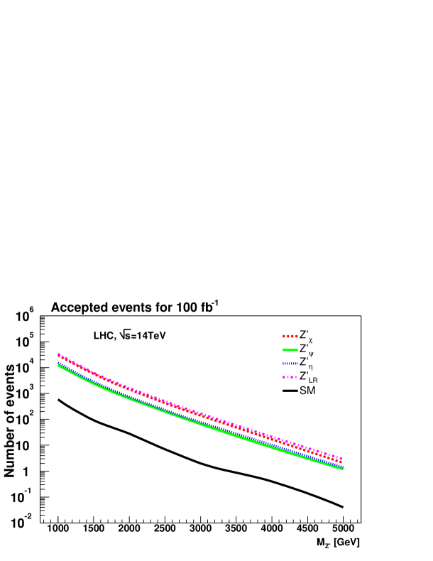
Figure 3: The LHC discovery reach: the number of events fulfilling the selection cuts for a luminosity of 100 fb^-1, for the different $Z^{\prime}$ models and in the SM case.

Figure 4a shows the invariant mass distribution for the dilepton system, as expected for different models with $M_{Z^{\prime}}$ fixed to 1.5 TeV and for the SM using a luminosity of 100 fb^-1. For all $Z^{\prime}$ models, huge peaks, corresponding to 3000–6000 signal events, are found above a small background. The cross sections for $Z^{\prime}$ bosons in the various models are also strongly varying.

In addition, very distinct observable forward-backward charge asymmetries are expected as a function of the dilepton mass and for the different $Z^{\prime}$ models, as shown in Fig. 4b. In order to get an impression of how an experimental signal with statistical fluctuations would look like, the measurable forward-backward asymmetry in the $Z^{\prime}_{\eta}$ case has been generated with the number of events corresponding to 100 fb^-1, as shown in Fig. 4b. We find that additional and complementary informations is also obtained from $A_{\rm FB}^{\ell}$ measured in the interference region. To quantify the study for a $Z^{\prime}$ mass of 1.5 TeV, “on-peak events” are counted if the dilepton mass is found in the interval $1.45$ TeV $\leq M_{\ell\ell}\leq$ 1.55 TeV. The “interference region” is defined accordingly and satisfy 1 TeV  $\leq M_{\ell\ell}\leq$ 1.45 TeV.

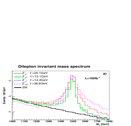
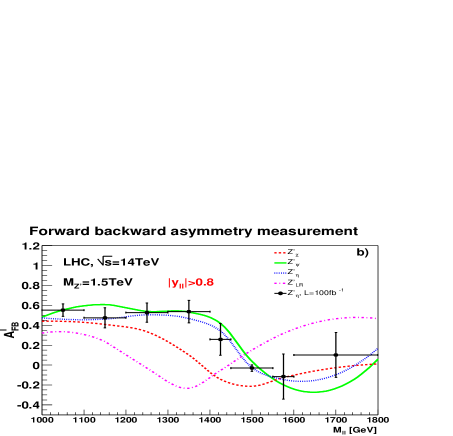
Figure 4: The dilepton invariant mass spectrum (a) and $A^{\ell}_{FB}$ (b) as a function of $M_{\ell\ell}$ for four $Z^{\prime}$ models. For the forward-backward charge asymmetry, the rapidity of the dilepton system is required to be larger than 0.8. A simulation of the statistical errors, including random fluctuations of the $Z^{\prime}_{\eta}$ model and with errors corresponding to a luminosity of 100 fb^-1 has been included in (b).

Finally, the rapidity distribution is analysed. Figure 5a shows the normalized distributions for a $Z^{\prime}$ with a mass of 1.5 TeV produced from $u\bar{u}$, $d\bar{d}$ and sea-antisea quark annihilation. Especially the $Z^{\prime}$ rapidity distribution from $u\bar{u}$ annihilation appears to be significantly different from the other two distributions. Figure 5b shows the expected rapidity distribution for the $Z^{\prime}_{\eta}$ model. A particular $Z^{\prime}$ rapidity distribution is fitted using a linear combination of the three pure quark-antiquark rapidity distributions shown in Fig. 5b. The fit output gives the $u\bar{u}$, $d\bar{d}$ and $sea$ quarks fraction in the sample. This will thus reveal how the $Z^{\prime}$ couples to different quark flavours in a particular model.

In order to demonstrate the analysis power of this method, we also show the rapidity distribution in the case of the $Z^{\prime}_{\psi}$ boson, which has equal couplings to up-type and down-type quarks. As can be qualitatively expected from the distributions shown in Fig. 5a, the used fitting procedure provides very accurate results for the known generated fraction $R_{u\bar{u}}$ of $u\bar{u}/$all, while some correlations between $d\bar{d}$ and the sea-antisea $Z^{\prime}$ production, which limits the accuracy of the measurement for the $d\bar{d}$ fractions. For example, for the $Z^{\prime}_{\eta}$ model, the generated event fractions from $u\bar{u}$, $d\bar{d}$ and sea-antisea quarks are 0.71, 0.26 and 0.03 respectively. The corresponding numbers from the fit and 100 fb^-1 are 0.71$\pm$0.07, 0.29$\pm$0.08 and 0.01$\pm$0.02.

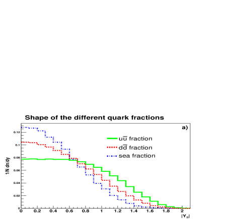
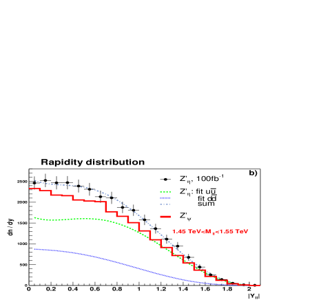
Figure 5: The normalized rapidity distribution of $Z^{\prime}$ with a mass of $1.5\pm 0.05$ TeV produced from the different types of quarks (a). The observable rapidity distribution for two different $Z^{\prime}$ models is shown in (b), including the fit results that determine the different types of $q\bar{q}$ fractions.

Table 2 shows the value of the cross section times the total decay width, the forward-backward charge asymmetry for the on-peak and interference regions as defined above, and the ratio of $Z^{\prime}$ events produced from $u\bar{u}$ annihilation as obtained from the fit to the $Z^{\prime}$ rapidity distribution.

Model	$\sigma^{3\Gamma}_{ll}\times\Gamma$ [fb$\cdot$GeV]			$A^{\rm on-peak}_{\rm FB}$			$A^{\rm off-peak}_{\rm FB}$			$R_{u\bar{u}}$
$Z^{\prime}_{\psi}$	487	$\pm$	5	0.04	$\pm$	0.03	0.53	$\pm$	0.04	0.60	$\pm$	0.07
$Z^{\prime}_{\eta}$	630	$\pm$	20	$-0.03$	$\pm$	0.03	0.45	$\pm$	0.04	0.71	$\pm$	0.07
$Z^{\prime}_{\chi}$	2050	$\pm$	40	$-0.23$	$\pm$	0.02	0.26	$\pm$	0.05	0.22	$\pm$	0.05
$Z^{\prime}_{LR}$	3630	$\pm$	80	0.15	$\pm$	0.02	0.06	$\pm$	0.06	0.45	$\pm$	0.05
$Z^{\prime}_{SM}$	8000	$\pm$	140	0.07	$\pm$	0.02	0.18	$\pm$	0.03	0.05	$\pm$	0.04
$Z^{\prime}_{d}$	1520	$\pm$	40	$-0.50$	$\pm$	0.02	0.26	$\pm$	0.05	0.00	$\pm$	0.01

Table 2: The values of the four basic observables, the signal cross section, multiplied by the total width, the forward-backward charge asymmetry on- and off-peak, and the ratio $R_{u\bar{u}}$ for various $Z^{\prime}$ models and with a $Z^{\prime}$ mass of 1.5 TeV. The quoted statistical errors are those that can be expected for a luminosity of 100 fb^-1.

4. Distinction between models and parameter determination

Let us now discuss how well the different $Z^{\prime}$ models can be distinguished experimentally using the observables defined before: $\sigma^{3\Gamma}_{\ell\ell}\times\Gamma$, $A_{\rm FB}^{\ell}$ on- and off-peak, as well as $R_{u\bar{u}}$ as obtained from the rapidity distribution. As a working hypothesis, a luminosity of 100 fb^-1 and a $Z^{\prime}$ mass of 1.5 TeV will be assumed in the following.

A precise knowledge of the cross section times the total width allows a first good distinction to be made between some models, as shown in the upper two plots of Fig. 6. It is not obvious how accurately absolute cross sections can be measured and interpreted at the LHC. However, following the procedure outlined in [17], comparable reactions, in this case $Z^{\prime}$ and $Z$ boson production, should be counted with respect to each other. The use of such ratio measurements should allow us to minimize systematic uncertainties, and an accuracy of $\pm$1% might be achievable. As can be seen from the other plots in Fig. 6, the additional variables show a different sensitivity for the different couplings.

For example, very similar cross sections are expected for the $E_{6}$ $Z^{\prime}$ models with $\cos\beta\sim\pm 1$ and for left-right models with $\alpha_{LR}\raisebox{-3.69899pt}{~{}\shortstack{$<$ \\ [-0.07cm] $\sim$}}~{}1.3$. However, these two different models show a very different behaviour for on- and especially off-peak asymmetries and for the couplings to up-type and down-type quarks. Obviously, the maximum sensitivity can be obtained by using all observables together. Having said this, one also needs to point out that some ambiguities between the different models remain, even after a complete analysis of 100 fb^-1 of data.

Assuming that a particular model has been selected, one would like to know how well the parameter(s), such as $\cos\beta$ or $\alpha_{LR}$, can be constrained. In the case of the $E_{6}$ model for instance, one finds that $\cos\beta$ cannot always be determined unambiguously. Very similar results can be expected for different observables but using very different values for $\cos\beta$. Again, the combination of the various measurements helps to reduce some ambiguities.

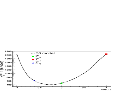
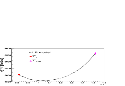
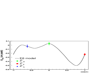
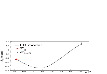
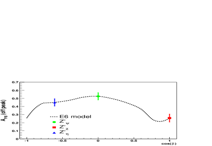
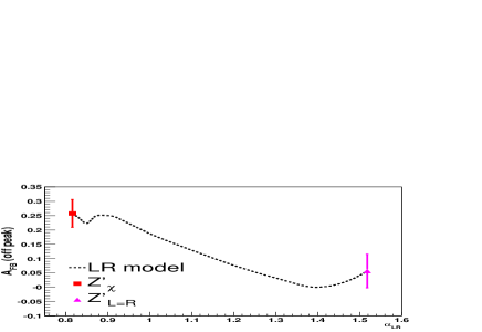
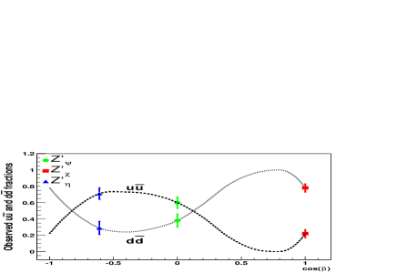
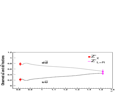
Figure 6: Variation of $\sigma^{3\Gamma}_{\ell\ell}\cdot\Gamma$, $A^{\rm on-peak}_{FB}$, $A^{\rm off-peak}_{FB}$ and the ratio $R_{q\bar{q}}$ as a function of the $E_{6}$ model parameter $\cos\beta$ (left) and the LR-model parameter $\alpha_{LR}$. The points corresponding to the particular $Z^{\prime}$ models are also shown.

If the $Z^{\prime}$ mass is increased, the number of events decreases drastically and the differences between the models start to become covered within the statistical fluctuations. For the assumed luminosity of 100 fb^-1, we could still distinguish a $Z^{\prime}_{\chi}$ from a $Z^{\prime}_{LR}$ over a large parameter range; the $A_{\rm FB}^{\ell}$ measurements provide some statistical significance up to $M_{Z^{\prime}}=2$–$2.5$ TeV. On the contrary, a $Z^{\prime}_{\eta}$ could be differentiated from a $Z^{\prime}_{\psi}$ only up to a $Z^{\prime}$ mass of at most 2 TeV as, in that case, the dependence of $A_{\rm FB}^{\ell}$ is almost identical in the two models.

In summary, a realistic simulation of the study of the properties of $Z^{\prime}$ bosons originating from various theoretical models has been performed for the LHC. We have shown that, in addition to the $Z^{\prime}$ production cross section times total decay width, the measurement of the forward-backward lepton charge asymmetry, both on the $Z^{\prime}$ peak and in the interference region, provide complementary information. We have also shown that a fit of the rapidity distribution can provide a sensitivity to the $Z^{\prime}$ couplings to up-type and down-type quarks. The combination of all these observables would allow us to discriminate between $Z^{\prime}$ bosons of different models or classes of models for masses up to 2–2.5 TeV, if a luminosity of 100 fb^-1 is collected.

Acknowledgements: We thank J. Hewett, G. Polesello and T. Rizzo for helpfull discussions during the Les Houches Workshop.

References

- [1] The LEP Electroweak Working Group and the SLD Heavy Flavour Group, Note LEPEWWG/2003-01; http://lepewwg.web.cern.ch/LEPEWWG.
- [2] See for instance, M. Cvetič et al., Phys. Rev. D56 (1997) 2861.
- [3] J. Hewett and T. Rizzo, Phys. Rep. 183 (1989) 193; A. Leike, Phys. Rep. 317 (1999) 143; M. Cvetič and P. Langacker, hep-ph/9707451.
- [4] See for instance, C. Hill and E. Simmons, hep-ph/0203079.
- [5] N. Arkani-Hamed et al., JHEP 0208 (2002) 021. For the phenomenological aspects, see: T. Han et al., Phys. Rev. D67 (2003) 095004; J. Hewett, F. Petriello and T. Rizzo, hep-ph/0211218; C. Csaki et al., hep-ph/0303236.
- [6] R. Casalbuoni et al., Phys. Lett. B460 (1999) 135; J. Rosner, Phys. Rev. D61 (2000) 016006; J. Erler and P. Langacker, Phys. Rev. Lett. 84 (2000) 212.
- [7] For an account, see J. Erler and P. Langacker, Phys. Lett. B456 (1999) 69; see also for an updated analysis of LEP1 limits, F. Richard, hep-ph/0303107.
- [8] M. Cvetič, S. Godfrey et al., DPF study in “Electroweak Symmetry Breaking and Beyond the Standard Model”, hep–ph/9504216; T.G. Rizzo, hep–ph/9612440; S. Godfrey, in APS/DPF/DPB Snowmass Study, hep-ph/0201092 and hep-ph/0201093.
- [9] R. Robinett and J. Rosner, Phys. Rev. D25 (1982) 3036; (E) ibid. D27 (1983) 679.
- [10] Proc. of the ECFA Large Hadron Collider Worshop, Aachen (Germany) 1990, Reports CERN 90–10 and ECFA 90–133.
- [11] CMS Collaboration, G.L. Bayatian et al., Technical Proposal, CERN/LHCC 94–38, LHCC/P1, 15 Dec. 1994.
- [12] ATLAS, Letter of Intent, CERN/LHCC 92-3 and ATLAS Collaboration, W. Armstrong et al.; Technical Proposal, CERN/LHCC 94-43, LHCC/P2, Dec. 1994.
- [13] A. Djouadi et al., Z. Phys. C56 (1992) 289.
- [14] P. Langacker, R. Robinett and J. Rosner, Phys. Rev. D30 (1984) 1470; V. Barger et al., Phys. Rev. D35 (1987) 2893; J. Rosner, Phys. Rev. D35 (1987) 2244.
- [15] M. Dittmar, Phys. Rev. D55 (1997) 161.
- [16] F. del Aguila, M. Cvetič and P. Langacker, Phys. Rev. D48 (1993) R969.
- [17] M. Dittmar, F. Pauss and D. Zürcher, Phys. Rev. D56 (1997) 7284.
- [18] T. Sjöstrand et al., Comput. Phys. Commun. 135 (2001) 238.
- [19] G. Azuelos and G. Polesello, hep–ph/0204031; see also, T. Rizzo, hep–ph/0305077.
- [20] J. Hewett and T. Rizzo in Ref. [3]. See also, A. Djouadi, Z. Phys. C63 (1994) 317; A. Djouadi and G. Azuelos, Z. Phys. C63 (1994) 327.
- [21] H. L. Lai et al. [CTEQ Collaboration], Eur. Phys. J. C 12 (2000) 375.
- [22] G. Altarelli, R. Ellis and G. Martinelli, Nucl. Phys. B143 (1978) 521 and B146 (1978) 544; J. Kubar–André and F. Paige, Phys. Rev. D19 (1979) 221.