Abstract

We analyze the partial decay widths of sfermions decaying into charginos and neutralinos $\Gamma({\tilde{f}}\to f^{\prime}\chi)$ at the one-loop level, including the electroweak and strong corrections. We present the renormalization framework, and discuss the value of the corrections. Since these corrections show non-decoupling effects, we analyze the radiative effects induced by a heavy squark sector into the lepton-slepton-chargino/neutralino couplings. We conclude that some knowledge of the heavy sector is needed in order to provide a sufficiently precise prediction for slepton observables at an $e^{+}e^{-}$ Linear Collider.

1 Introduction

One of the basic predictions of Supersymmetry (SUSY) is the equality between the couplings of SM particles and that of their superpartners. The simplest processes in which this prediction could be tested is the partial decay widths of sfermions into Standard Model (SM) fermions and charginos/neutralinos:

$$\Gamma({\tilde{f}}\to f^{\prime}\chi)\,\,.$$ (1)

By measuring these partial decay widths (or the corresponding branching ratios) one could measure the fermion-sfermion-chargino/neutralino Yukawa couplings and compare them with the SM fermion gauge couplings. The $e^{+}e^{-}$ Linear Collider (LC) is an ideal machine where these test can be performed, with a precision below the percent level.

We have computed the full one-loop electroweak corrections to the partial decay widths (1). As we will show, the radiative corrections induce finite shifts in the couplings which are non-decoupling.

The QCD corrections to the process (1) were computed in [1], and the Yukawa corrections to bottom-squarks decaying into charginos was given in [2]. Here we present the last step, namely, the full electroweak corrections in the framework of the Minimal Supersymmetric Standard Model (MSSM). Full details of the present work can be found in [3]. The present note complements and supersedes Ref. [4].

2 Renormalization and radiative corrections

The computation to one-loop level of the partial decay width (1) requires the renormalization of the full MSSM Lagrangian, taking into account the relations among the different sectors and the mixing parameters. We choose to work in an on-shell renormalization scheme, in which the renormalized parameters are the measured quantities. The SM sector is renormalized according to the standard on-shell SM $\alpha$-scheme [5], and the MSSM Higgs sector (in particular the renormalization of $\tan\beta$) is treated as in [6].

As far as the sfermion sector is concerned, we follow the procedure described in [2]. However, in the present analysis we treat simultaneously top-squarks and bottom-squarks. Due to $SU(2)_{L}$ invariance the parameters in these two sectors are not independent, and we can not supply with independent on-shell conditions for both sectors. We choose as input parameters the on-shell masses of both bottom-squarks, the lightest top-squark mass, and the mixing angles in both sectors:

$$(m_{\tilde{b}_{1}},m_{\tilde{b}_{2}},\theta_{b},m_{\tilde{t}_{2}},\theta_{t}),\ \ \ \ m_{{\tilde{f}}_{1}}>m_{{\tilde{f}}_{2}}.$$ (2)

The remaining parameters are computed as a function of those in (2). In particular, the trilinear soft-SUSY-breaking couplings read:

$$A_{\{b,t\}}=\mu\{\tan\beta,\cot\beta\}+{m_{\tilde{f}_{1}}^{2}-m_{\tilde{f}_{2}}^{2}\over 2\,m_{f}}\,\sin{2\,\theta_{f}}\,,$$ (3)

with $\tan\beta=v_{2}/v_{1}$, the ratio of the vacuum expectation values of the two Higgs boson doublets. The approximate (necessary) condition to avoid colour-breaking minima in the MSSM Higgs potential [7],

$$A_{q}^{2}<3\,(m_{\tilde{t}}^{2}+m_{\tilde{b}}^{2}+M_{H}^{2}+\mu^{2})\,,$$ (4)

imposes a tight correlation between the sfermion mass splitting and the mixing angle at large $\tan\beta$. Since the heaviest top-squark mass ($m_{\tilde{t}_{1}}$) is not an input parameter, it receives finite radiative corrections:

$$\Delta m_{\tilde{t}_{1}}^{2}=\delta m_{\tilde{t}_{1}}^{2}+\Sigma_{\tilde{t}_{1}}(m_{\tilde{t}_{1}}^{2})\,\,,$$ (5)

where $\delta m_{\tilde{t}_{1}}^{2}$ is a combination of the counterterms of the parameters in (2), and the counterterms of the gauge and Higgs sectors.

The chargino/neutralino sector contains six particles, but only three independent input parameters: the soft-SUSY-breaking $SU(2)_{L}$ and $U(1)_{Y}$ gaugino masses ($M$ and $M^{\prime}$), and the higgsino mass parameter ($\mu$). The situation in this sector is quite different from the sfermion case, since in this case no independent counterterms for the mixing matrix elements can be introduced. We stick to the following procedure: First, we introduce a set of renormalized parameters $(M,M^{\prime},\mu)$ in the expression of the chargino and neutralino matrices ($\cal{M}$ and ${\cal M}^{0}$), and diagonalize them by means of unitary matrices $M_{D}=U^{*}{\cal M}V^{\dagger}$, $M_{D}^{0}=N^{*}{\cal M}^{0}N^{\dagger}$. Now $U$, $V$ and $N$ must be regarded as renormalized mixing matrices. The counterterm mass matrices are then $\delta M_{D}=U^{*}\delta{\cal M}V^{\dagger}$, $\delta M_{D}^{0}=N^{*}\delta{\cal M}^{0}N^{\dagger}$, which are non-diagonal. At this point, we introduce renormalization conditions for certain elements of $\delta M_{D}$ and $\delta M_{D}^{0}$. In particular, we use on-shell renormalization conditions for the two chargino masses ($M_{1}$ and $M_{2}$), which allows to compute the counterterms $\delta M$ and $\delta\mu$. This information, together with the on-shell condition for the lightest neutralino mass ($M_{1}^{0}$) allows to derive the expression for the counterterm $\delta M^{\prime}$. The other neutralino masses ($M_{2,3,4}^{0}$) receive radiative corrections. In this framework the renormalized one-loop chargino/neutralino 2-point functions are non-diagonal. Therefore one must take into account this mixing either by including explicitly the reducible $\chi_{r}-\chi_{s}$ mixing diagrams, or by means of external mixing wave-function terms (${\cal Z}_{\{L,R\}}^{0\beta\alpha}$, ${\cal Z}_{\{L,R\}}^{-ij}$). See Refs. [8] for different (but one-loop equivalent) approaches to the renormalization of the chargino/neutralino sector.

The complete one-loop computation consists of:

• renormalization constants for the parameters and wave functions in the bare Lagrangian,

• one-loop one-particle irreducible three-point functions,

• mixing terms among the external charginos and neutralinos,

• soft- and hard- photon bremsstrahlung.

All kind of MSSM particles are taken into account in the loops: SM fermions, sfermions, electroweak gauge bosons, Higgs bosons, Goldstone bosons, Fadeev-Popov ghosts, charginos, neutralinos. The computation is performed in the ’t Hooft-Feynman gauge, using dimensional reduction for the regularization of divergent integrals. The loop computation itself is done using the computer algebra packages FeynArts 3.0 and FormCalc 2.2 [10, 11]. The numerical evaluation of one-loop integrals makes use of LoopTools 1.2 [11].

3 Results

The results show the very interesting property that none of the particles of the MSSM decouples from the corrections to the observables (1). This can be well understood in terms of renormalization group (RG) running of the parameters and SUSY breaking. Take, e.g., the effects of squarks in the electron-selectron-photino coupling. Above the squark mass scale ($Q>m_{\tilde{q}}$) the electron electromagnetic coupling ($\alpha(Q)$) is equal (by SUSY) to the electron-selectron-photino coupling ($\tilde{\alpha}(Q)$), and both couplings run according to the same RG equations. At $Q=m_{\tilde{q}}$ the squarks decouple from the RG running of the couplings. At $Q<m_{\tilde{q}}$, $\alpha(Q)$ runs due to the contributions from pure quark loops, but $\tilde{\alpha}(Q)$ does not run anymore, and it is frozen at the squark scale, that is: $\tilde{\alpha}(Q<m_{\tilde{q}})=\alpha(m_{\tilde{q}})$. Therefore, when comparing these two couplings at a scale $Q<m_{\tilde{q}}$, they differ by the logarithmic running of $\alpha(Q)$ from the squark scale to $Q$: $\tilde{\alpha}(Q)/\alpha(Q)-1=\beta\log(m_{\tilde{q}}/Q)$.

The above discussion has two important consequences:

1. The non-decoupling can be used to extract information of the high-energy part of the SUSY spectrum: one can envisage a SUSY model in which a significant splitting among the different SUSY masses exists, e.g. $m_{\tilde{q}}\gg m_{\tilde{l}}$, where the sleptons lie below the production threshold in an $e^{+}e^{-}$ linear collider, but the squarks are above it. By means of high precision measurements of the lepton-slepton-chargino/neutralino couplings one might be able to extract information of the squark sector of the model, to be checked with the available data from the LHC.

2. By the same token, it means that the value of the radiative corrections depends on all parameters of the model, and we can not make precise quantitative statements unless the full SUSY spectrum is known. This drawback can be partially overcome by the introduction of effective coupling matrices, which can be defined as follows. The subset of fermion-sfermion one-loop contributions to the self-energies of gauge-boson, Higgs-bosons, Goldstone-bosons, charginos and neutralinos form a gauge invariant finite subset of the corrections. Therefore these contributions can be absorbed into a finite shift of the chargino/neutralino mixing matrices $U$, $V$ and $N$ appearing in the couplings:

   $$U^{eff}=U+\Delta U^{(f)},\ V^{eff}=V+\Delta V^{(f)},\ N^{eff}=N+\Delta N^{(f)}.$$ (6)

   In this way we can decouple the computation of the universal (or super-oblique [13]) corrections. These corrections contain the non-decoupling logarithms from sfermion masses.

As an example of the universal corrections we have computed the electron-selectron contributions to the $\Delta U^{(f)}$ and $\Delta V^{(f)}$ matrices, assuming zero mixing angle in the selectron sector ($\theta_{e}=0$), we have identified the leading terms in the approximation $m_{\tilde{e}_{i}},m_{\tilde{\nu}}\gg(M_{W},M_{i})\gg m_{e}$, and analytically canceled the divergences and the renormalization scale dependent terms; finally, we have kept only the terms logarithmic in the slepton masses. The result for $\Delta U^{(f)}$ reads as follows:

$$\Delta U_{i1}^{(f)} = \frac{\alpha}{4\,\pi\,s_{W}^{2}}\log\left(\frac{M^{2}_{\tilde{e}_{L}}}{M^{2}_{X}}\right)\,\bigg{[}\frac{U_{i1}^{3}}{6}-U_{i2}\frac{\sqrt{2}\,M_{W}\,(M\,c_{\beta}+\mu\,s_{\beta})}{3\,(M^{2}-\mu^{2})\,\left(M_{1}^{2}-M_{2}^{2}\right)^{2}}\left(M^{4}-M^{2}\,\mu^{2}+\right.$$

$$\left.+3\,M^{2}\,M^{2}_{W}+\mu^{2}\,M^{2}_{W}+{M_{W}^{4}}+{M_{W}^{4}}\,c_{4\beta}+(\mu^{2}-M^{2})\,M^{2}_{i}+4\,M\,\mu\,M^{2}_{W}\,s_{2\beta}\right)\,\bigg{]}\,\,,$$

$$\Delta U_{i2}^{(f)} = \frac{\alpha}{4\,\pi\,s_{W}^{2}}\log\left(\frac{M^{2}_{\tilde{e}_{L}}}{M^{2}_{X}}\right)\,U_{i1}\,\frac{M_{W}\,(M\,c_{\beta}+\mu\,s_{\beta})}{3\,\sqrt{2}\,(M^{2}-\mu^{2})\,\left(M_{1}^{2}-M_{2}^{2}\right)^{2}}\times$$ (7)

$$\times \left((M^{2}-\mu^{2})^{2}+4\,M^{2}\,M^{2}_{W}+4\,\mu^{2}\,M^{2}_{W}+2\,{M_{W}^{4}}+2\,{M_{W}^{4}}\,c_{4\beta}+8\,M\,\mu\,M^{2}_{W}\,s_{2\beta}\right)\,\,,$$

$M^{2}_{\tilde{e}_{L}}$ being the soft-SUSY-breaking mass of the $(\tilde{e}_{L},\tilde{\nu})$ doublet, whereas $M_{X}$ is a SM mass. In the on-shell scheme for the SM electroweak theory we define parameters at very different scales, basically $M_{X}=M_{W}$ and $M_{X}=m_{e}$. These wide-ranging scales enter the structure of the counterterms and so must appear in eq.(7) too. As a result the leading log in the various terms of this equation will vary accordingly. For simplicity in the notation we have factorized $\log M^{2}_{\tilde{e}_{L}}/M^{2}_{X}$ as an overall factor. In some cases this factor can be very big, $\log M^{2}_{\tilde{e}_{L}}/m_{e}^{2}$; it comes from the electron-selectron contribution to the chargino-neutralino self-energies.

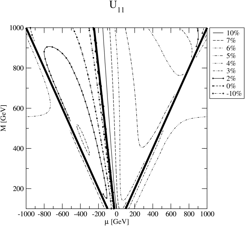
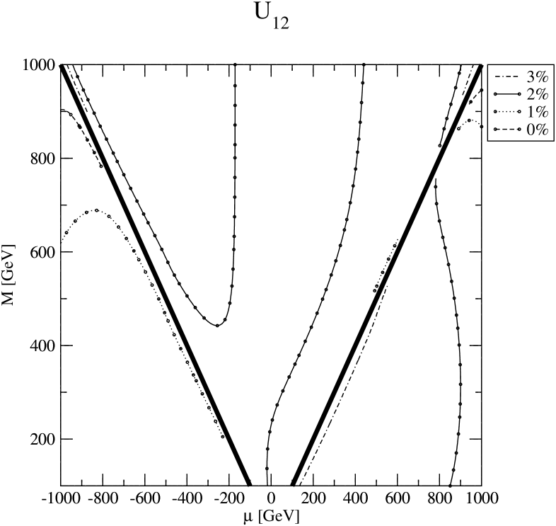
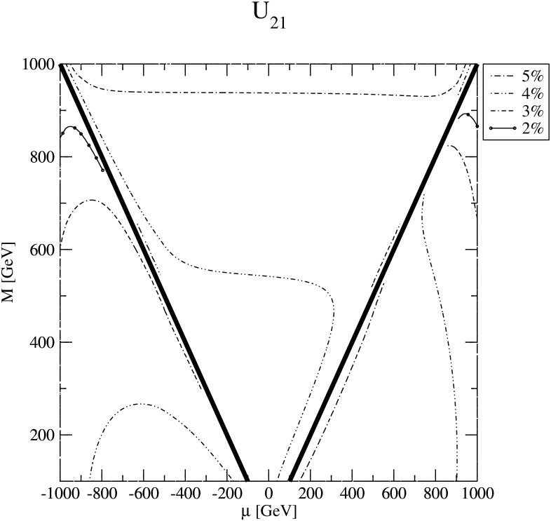
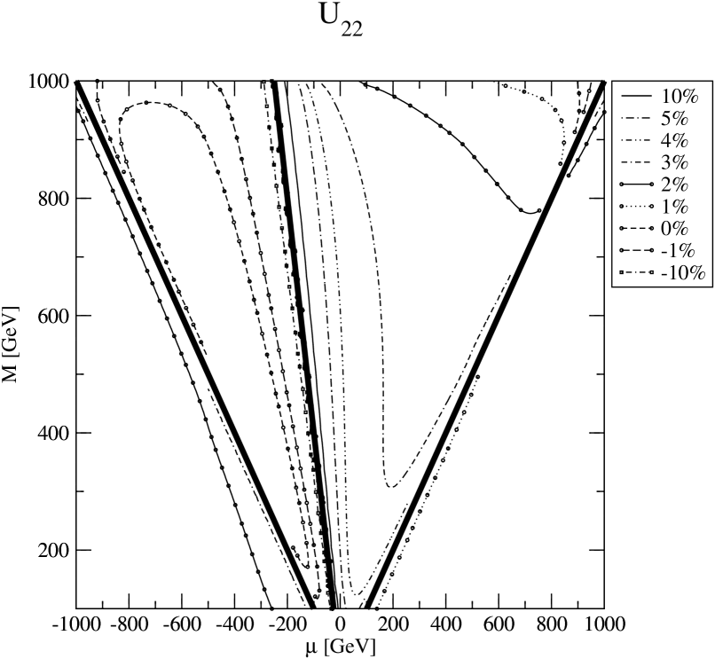
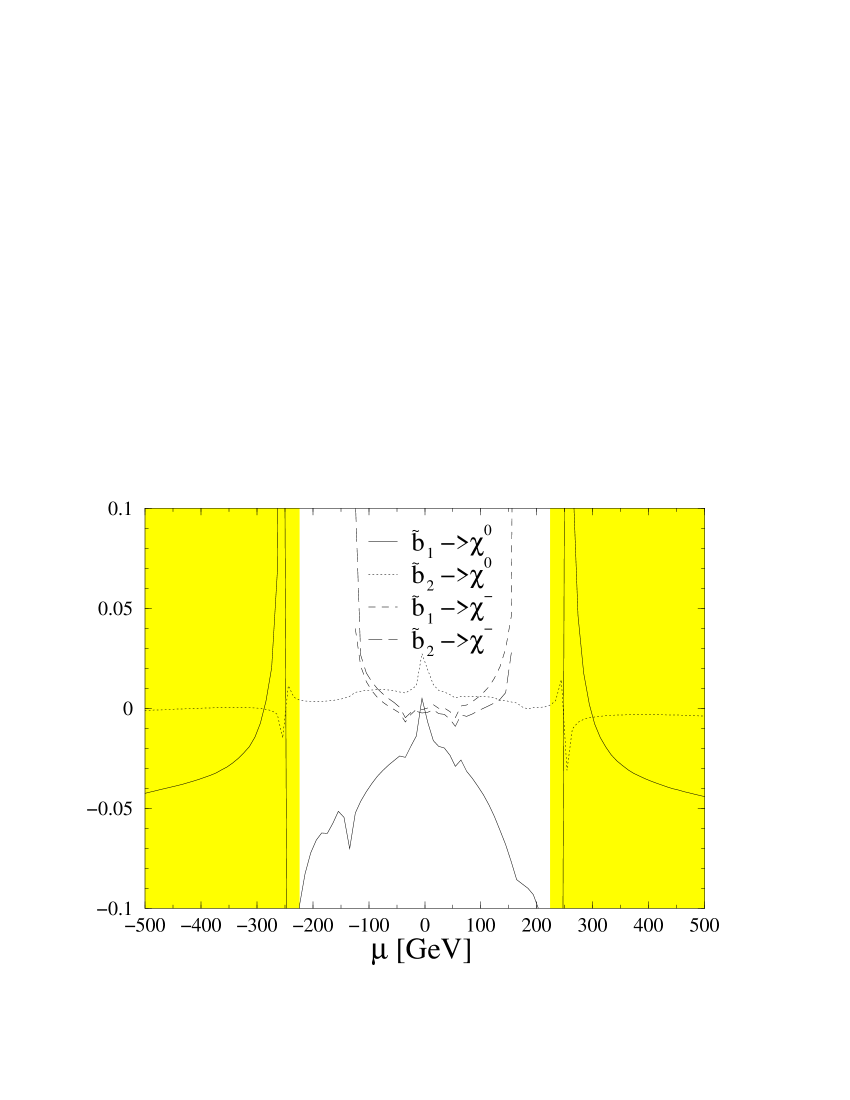
In Fig. 1 we show the relative correction to the matrix elements of $U$ for a sfermion spectrum around $1\mbox{ TeV}$. The thick black lines in Fig. 1 correspond to spurious divergences in the relative corrections due to the renormalization prescriptions. Corrections as large as $\pm 10\%$ can only be found in the vicinity of these divergence lines. However, there exist large regions of the $\mu-M$ plane where the corrections are larger than $2\%$, $3\%$, or even $4\%$.

Figure 1: Relative correction to the effective chargino coupling matrix $\Delta U^{(f)}/U$ in the $M-\mu$ plane, for $\tan\beta=4$ and a sfermion spectrum around $1\mbox{ TeV}$ ($m_{\tilde{l}_{2}}=m_{\tilde{d}_{2}}=m_{\tilde{u}_{2}}=1\mbox{ TeV}\,,\,m_{\tilde{l}_{1}}=m_{\tilde{d}_{1}}=m_{\tilde{l}_{2}}+5\mbox{ GeV}\,,\,\theta_{l}=\theta_{q}=\theta_{b}=0\,,\,\theta_{t}=-\pi/5$).

The effects of the universal corrections to the partial decay widths (1) are shown in Fig. 2 for top- and bottom-squark decays as a function of a common slepton mass.

(a)	(b)

Figure 2: Universal relative corrections (8) to third generation squark partial decay widths as a function of a common slepton mass using the input parameter set (9).

Here (and in most of the discussion below) we show the corrections to the total decay widths of sfermions into charginos and neutralinos, that is

$$\delta(\tilde{f_{a}}\to f^{\prime}\chi)=\frac{\sum_{r}\left(\Gamma(\tilde{f_{a}}\to f^{\prime}\chi_{r})-\Gamma^{0}(\tilde{f_{a}}\to f^{\prime}\chi_{r})\right)}{\sum_{r}\Gamma^{0}(\tilde{f_{a}}\to f^{\prime}\chi_{r})}\,\,,$$ (8)

with $\chi=\chi^{\pm}$ or $\chi=\chi^{0}$. We will not show results for processes whose branching ratio are less that 10% in all of the explored parameter space. The default parameter set used is:

$$\begin{array}[]{l}\tan\beta=4\,\,,m_{t}=175\mbox{ GeV}\,\,,m_{b}=5\mbox{ GeV}\,\,,m_{\tilde{b}_{2}}=m_{\tilde{d}_{2}}=m_{\tilde{u}_{2}}=m_{\tilde{e}_{2}}=300\mbox{ GeV}\,\,,\\ m_{\tilde{b}_{1}}=m_{\tilde{d}_{1}}=m_{\tilde{e}_{1}}=m_{\tilde{b}_{2}}+5\mbox{ GeV}\,\,,m_{\tilde{u}_{2}}=290\mbox{ GeV}\,\,,m_{\tilde{t}_{2}}=300\mbox{ GeV}\,\,,\\ \theta_{b}=\theta_{d}=\theta_{u}=\theta_{e}=0\,\,,\theta_{t}=-\pi/5\,\,,\mu=150\mbox{ GeV}\,\,,M=250\mbox{ GeV}\,\,,M_{H^{\pm}}=120\mbox{ GeV}\,\,,\end{array}$$ (9)

The logarithmic behaviour from eq. (7) is evident in this figure. The logarithmic regime is attained already for slepton masses of order $1\mbox{ TeV}$. The universal corrections are seen to be positive for all squark decays, ranging between $4\%$ and $7\%$ for slepton masses below $1\mbox{ TeV}$.

Although above we have singled out the non-decoupling properties of sfermions, we would like to stress that the whole spectrum shows non-decoupling properties. By numerical analysis we have been able to show the existence of logarithms of the gaugino mass parameters ($M/M_{X}$ and $M^{\prime}/M_{X}$), and the Higgs mass ($M_{H^{\pm}}/M_{X}$). However, due to the complicated mixing structure of the model, we were not able to derive simple analytic expressions containing these non-decoupling logarithms. Note that in any observable which includes the fermion-sfermion-chargino/neutralino Yukawa couplings at leading order we will have this kind of corrections, therefore the full MSSM spectrum must be taken into account when computing radiative corrections, since otherwise one could be missing large logarithmic contributions of the heavy masses.

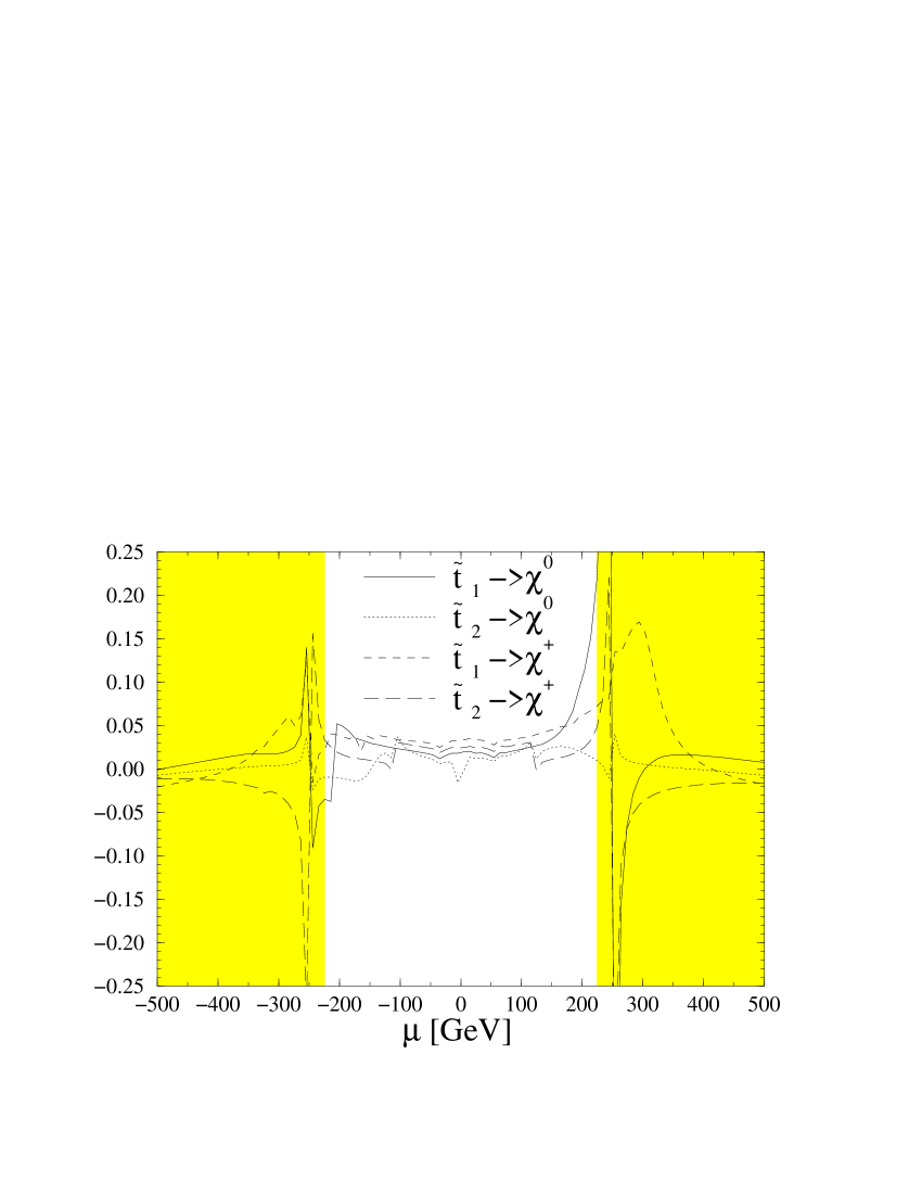
As for the non-universal part of the contributions, they show a rich structure, as can be seen in Fig. 3. There we show the evolution of the corrections as a function of the $\mu$ parameter for top- and bottom-squark decays. A number of divergences are seen in the figure, ones related to the mass renormalization framework (at $|\mu|=M$), and others due to threshold singularities in the external wave function renormalization constants. It is clear that the precise value of the corrections is very much dependent on the correlation among the different SUSY masses.

(a)	(b)

Figure 3: Non-universal corrections to the partial decay width of top- and bottom-squarks as a function of the higgsino mass parameter $\mu$. The shaded regions correspond to the violation of the condition (4).

An important contribution to the corrections of third-generation sfermion decays is the threshold correction to the bottom-quark ($\tau$-lepton) Yukawa coupling ($\Delta m_{\{b,\tau\}}$) [14]. In the processes under study (1) two kind of contributions appear: first, the genuine corrections $\Delta m_{\{b,\tau\}}$ from SUSY loops in the fermion self-energy; and second in the loops of sfermion self-energies mixing different chiral states ${\tilde{f}}_{L}\leftrightarrow{\tilde{f}}_{R}$. This kind of corrections grow with the sfermion mass splitting, the sfermion mixing angle, and $\tan\beta$.

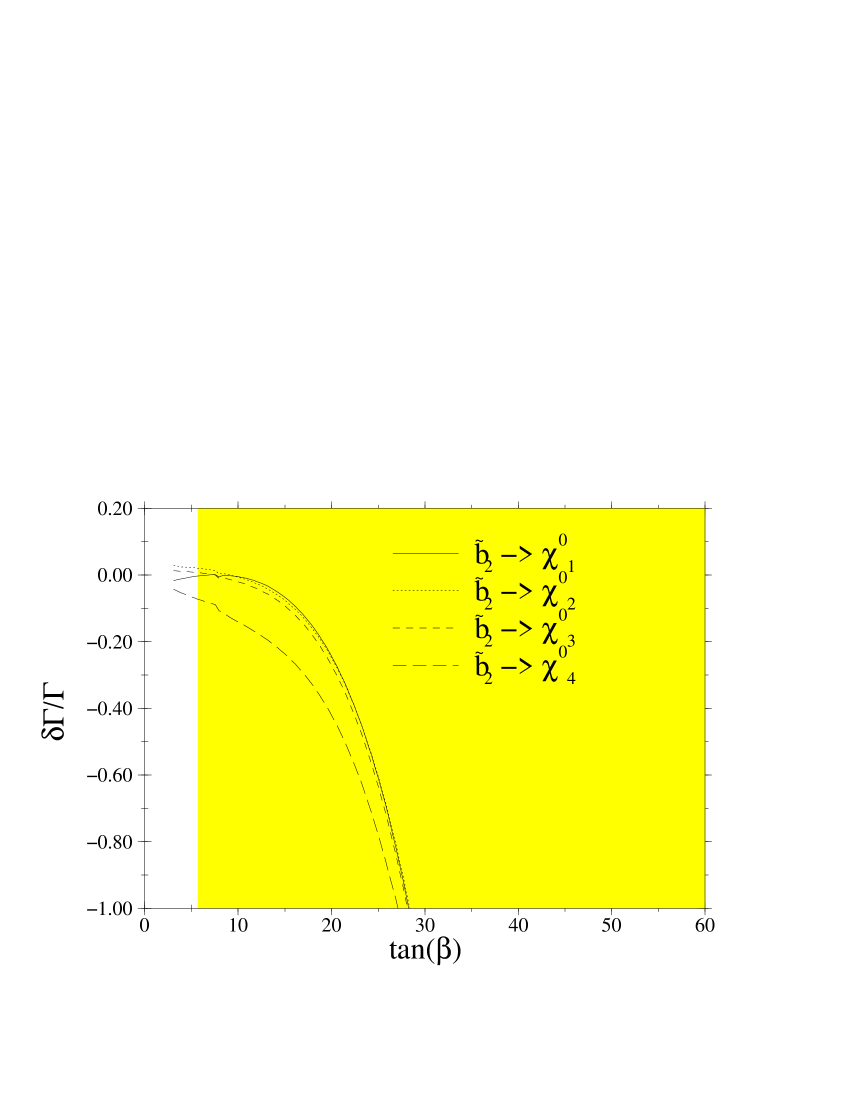
A complementary set of corrections corresponds to the genuine three-point vertex functions including Higgs bosons in the loops. These contributions are proportional to the soft SUSY-breaking trilinear couplings (3), and therefore potentially large. Concretely, if $\tan\beta$ is large, and the bottom-squark mass splitting (or the mixing angle) is small, the bottom-squark trilinear coupling grows with $\tan\beta$ ($A_{b}\simeq\mu\tan\beta$), eventually inducing corrections larger than $100\%$, spoiling the validity of perturbation theory. In Fig. 4a we show the evolution of the corrections to the lightest bottom-squark decay into neutralinos as a function of $\tan\beta$ using the parameter set (9). We see the fast growing of the corrections, reaching $-100\%$ at $\tan\beta\simeq 30$. Fortunately, applying the (necessary) restriction (4) keeps the $A_{q}$ parameter small. In Fig. 4b we show again the evolution of the corrections as a function of $\tan\beta$, but this time keeping a fixed value for the trilinear couplings $A_{b}=600\mbox{ GeV}$, $A_{t}=-78\mbox{ GeV}$. The figure shows that the corrections stay well below $10\%$ all over the $\tan\beta$ range for this channel.

The complementarity between the $\Delta m_{\{b,\tau\}}$-like and the $A_{f}$-like corrections is as follows: at large $\tan\beta$, if the bottom-squark mass splitting is large, there will be large corrections of type $\Delta m_{\{b,\tau\}}$; on the other hand, if the bottom-squark mass splitting is small, there will be large corrections of the type $A_{f}$. Note that the QCD corrections contain $\Delta m_{b}$ terms but not $A_{f}$ terms. When analyzing QCD corrections alone, one could choose a small splitting, obtaining small corrections, however we have seen that this is inconsistent, so one is forced to a large $\Delta m_{b}^{QCD}$ contribution, which can reinforce (or screen) the negative corrections from the standard running of the QCD coupling constant.

(a)	(b)

Figure 4: Non-universal relative corrections to the lightest bottom-squark partial decays widths into neutralinos as a function of $\tan\beta$. a) Keeping fixed the splitting between the bottom-squarks $m_{\tilde{b}_{1}}-m_{\tilde{b}_{2}}=5\mbox{ GeV}$. b) Keeping $A_{b}=600\mbox{ GeV},A_{t}=-78\mbox{ GeV}$. The shaded region corresponds to the violation of the condition (4).

It is known that the electroweak corrections to any process grow as the logarithm squared of the process energy scale due to the Sudakov double-logs [15]. We have observed this behaviour in the process under study.

At the end of the day, we want to analyze the branching ratios, which are the true observables. For this analysis we have to add the QCD corrections to the EW corrections. Due to the large value of the QCD corrections, we made use of the enhanced resummed expression for the bottom-quark Yukawa coupling [16]. In Table 1 we show the tree-level and corrected branching ratios for top- and bottom-squarks using the input parameter set (9) and $m_{\tilde{g}}=500\mbox{ GeV}$. From inspection of Table 1 we see that the EW corrections can induce a change on the branching ratios of the leading decay channels of squarks comparable to the QCD corrections. Therefore both contributions must be taken into account on equal footing in the analysis of the phenomenology of sfermions.

	$\chi^{0}_{1}$	$\chi^{0}_{2}$	$\chi^{0}_{3}$	$\chi^{0}_{4}$	$\chi^{+}_{1}$	$\chi^{+}_{2}$
$BR^{tree}(\tilde{t}_{1}\to q\chi)$	0.169	0.249	0.145	-	0.159	0.278
$BR^{QCD}(\tilde{t}_{1}\to q\chi)$	0.164	0.257	0.144	-	0.099	0.335
$BR^{total}(\tilde{t}_{1}\to q\chi)$	0.177	0.242	0.143	-	0.122	0.316
$BR^{tree}(\tilde{t}_{2}\to q\chi)$	0.058	-	-	-	0.942	-
$BR^{QCD}(\tilde{t}_{2}\to q\chi)$	0.063	-	-	-	0.937	-
$BR^{total}(\tilde{t}_{2}\to q\chi)$	0.065	-	-	-	0.935	-
$BR^{tree}(\tilde{b}_{1}\to q\chi)$	0.272	0.092	0.047	0.014	0.575	-
$BR^{QCD}(\tilde{b}_{1}\to q\chi)$	0.308	0.104	0.031	0.018	0.538	-
$BR^{total}(\tilde{b}_{1}\to q\chi)$	0.291	0.092	0.031	0.018	0.568	-
$BR^{tree}(\tilde{b}_{2}\to q\chi)$	0.502	0.332	0.123	-	0.042	-
$BR^{QCD}(\tilde{b}_{2}\to q\chi)$	0.541	0.386	0.054	-	0.019	-
$BR^{total}(\tilde{b}_{2}\to q\chi)$	0.528	0.395	0.056	-	0.020	-

Table 1: Tree-level and corrected branching ratios of top- and bottom-squark decays into charginos and neutralinos for the parameter set (9) and $m_{\tilde{g}}=500\mbox{ GeV}$. Branching ratios below $10^{-3}$ are not shown.

4 Squark effects in sleptons observables

Since the corrections do not decouple by taking the large mass limit, the logical question appears: which knowledge of the heavy spectrum is necessary in order to provide a theoretical prediction with sufficient accuracy for the properties of the light particles? In the following we try to answer this question. To this end, we choose a spectrum with light sleptons and heavy squarks, and look at the radiative effects of the latter in the properties of the former. For the numerical analysis we choose as default parameters those of the Snowmass Points and Slopes (SPS), point 1a [17]. For completeness we give here the values of the soft-SUSY-breaking parameters for this point:

$$\begin{array}[]{l}\tan\beta=10,M_{A^{0}}=393.6\mbox{ GeV},\mu=352.4\mbox{ GeV},M=192.7\mbox{ GeV},M^{\prime}=99.1\mbox{ GeV}\,\,,\\ M_{\{\tilde{d},\tilde{s}\}_{L}}=539.9\mbox{ GeV},M_{\tilde{b}_{L}}=495.9\mbox{ GeV},M_{\{\tilde{d},\tilde{s}\}_{R}}=519.5\mbox{ GeV},M_{\tilde{b}_{R}}=516.9\mbox{ GeV},\\ A_{\{d,s\}}=3524\mbox{ GeV},A_{b}=-772.7\mbox{ GeV},\\ M_{\{\tilde{u},\tilde{c}\}_{R}}=521.7\mbox{ GeV},M_{\tilde{t}_{R}}=424.8\mbox{ GeV},A_{u,c}=35.24\mbox{ GeV},A_{t}=-510\mbox{ GeV},\\ M_{\{\tilde{e},\tilde{\mu}\}_{L}}=196.6\mbox{ GeV},M_{\tilde{\tau}_{L}}=195.8\mbox{ GeV},M_{\{\tilde{e},\tilde{\mu}\}_{R}}=136.2\mbox{ GeV},M_{\tilde{\tau}_{R}}=133.6\mbox{ GeV},\\ A_{e,\mu}=3524\mbox{ GeV},A_{\tau}=-254.2\mbox{ GeV},\end{array}$$ (10)

where the soft-SUSY-breaking trilinear couplings of the first and second generation sfermions have been chosen such that the non-diagonal elements of the sfermion mass matrix are zero.

However, a note of caution should be given, our computation is performed in the On-shell renormalization scheme, whereas the SPS parameters are given in the $\overline{DR}$ renormalization scheme, and one should make a scheme conversion of the parameters, this conversion is beyond the scope of the present work. In this note we are interested only in establishing whether the effects of heavy particles are important, and therefore we are only interested in obtaining a suitable SUSY spectrum, therefore we treat the given numerical parameters of SPS 1a as On-shell SUSY parameters .

	$\Gamma^{tree}$ [GeV]	$\delta\Gamma^{(q)}/\Gamma$	$\delta\Gamma^{(l)}/\Gamma$	$\delta\Gamma^{no-uni}/\Gamma$	$\delta\Gamma/\Gamma$
$\tilde{e}_{1}\to e^{-}\chi^{0}_{1}$	0.110	0.043	0.032	-0.002	0.073
$\tilde{e}_{1}\to e^{-}\chi^{0}_{2}$	0.047	0.030	0.034	-0.012	0.051
$\tilde{e}_{1}\to\nu_{e}\chi^{-}_{1}$	0.081	0.026	0.033	0.006	0.065
$\tilde{e}_{2}\to e^{-}\chi^{0}_{1}$	0.194	0.052	0.034	0.000	0.086
$\tilde{\nu}_{e}\to\nu_{e}\chi^{0}_{1}$	0.140	0.059	0.035	-0.005	0.089
$\tilde{\nu}_{e}\to\nu_{e}\chi^{0}_{2}$	0.006	0.018	0.033	-0.014	0.036
$\tilde{\nu}_{e}\to e^{-}\chi^{+}_{1}$	0.016	0.024	0.033	0.002	0.059

Table 2: Tree-level partial decay widths and relative corrections for the selectron and sneutrino decays into charginos and neutralinos for SPS 1a.

In the following we separate among three different kinds of contributions: $\delta\Gamma^{(q)}$ are the corrections induced by the quark-squark loops to the universal corrections in (6), and are the main subject of study in this section; $\delta\Gamma^{(l)}$ are the corrections induced by the lepton-slepton loops to the universal corrections in (6); $\delta\Gamma^{no-uni}$ are the non-universal corrections as before.

In Table 2 we show the partial decay widths of selectrons into charginos/neutralinos for SPS 1a. We show: the tree-level partial widths $\Gamma^{tree}$; the relative corrections induced by quarks-squarks $\delta\Gamma^{(q)}/\Gamma$; the relative corrections induced by the lepton-slepton universal contributions $\delta\Gamma^{(l)}/\Gamma$; the process-dependent non-universal contributions $\delta\Gamma^{no-uni}/\Gamma$; and the total corrections $\delta\Gamma/\Gamma$.

The universal corrections $\delta\Gamma^{(q)}/\Gamma$ and $\delta\Gamma^{(l)}/\Gamma$ in Table 2 represent a correction that will be present whenever a fermion-sfermion-chargino/neutralino coupling enters a given observable. The correction $\delta\Gamma^{no-uni}/\Gamma$ represents the process-dependent part. For the presented observables the non-universal corrections turn out to be quite small, but this is not necessarily always the case. From the values of Table 2 it is clear that the corrections of the quark-squark sector are as large as the corrections from the (light) lepton-slepton sector, for the presented observables they amount to a $2-6\%$ relative correction, depending on the particular decay channel.

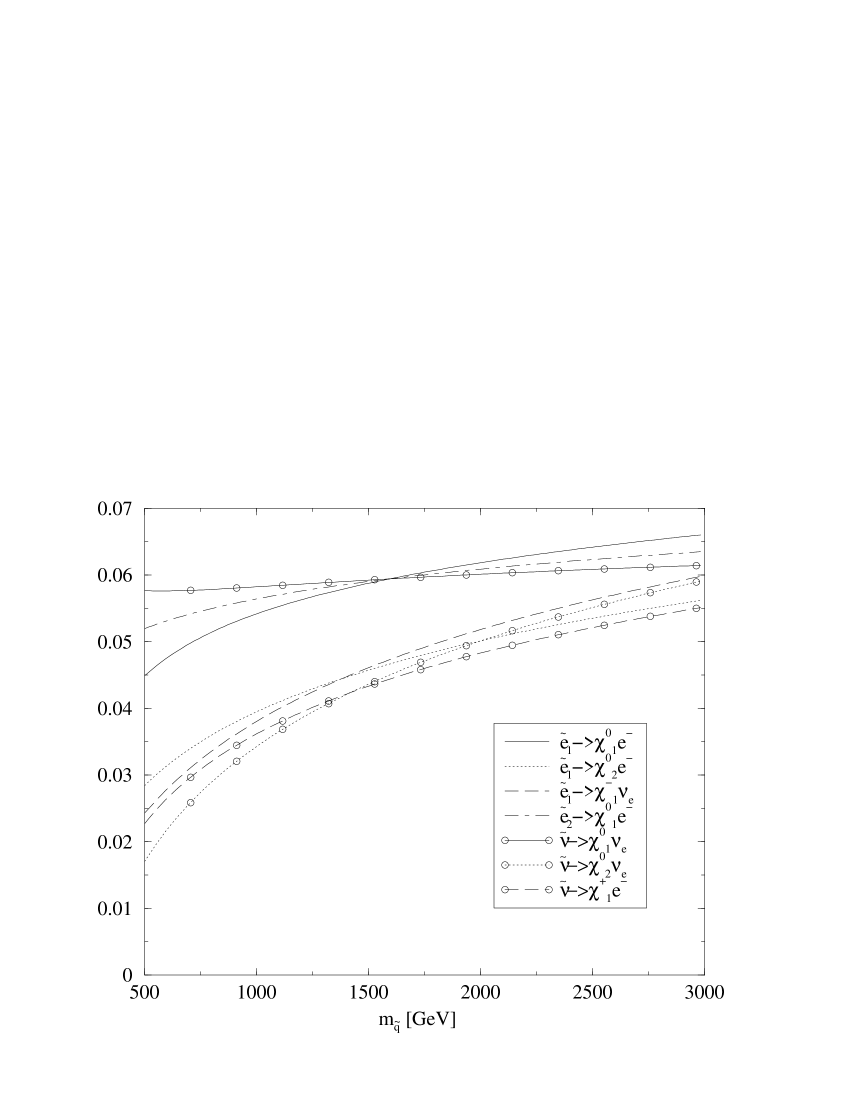
For SPS 1a the squark mass scale is around 500 GeV, however the corrections grow logarithmically with the squark mass scale. In Fig. 5 we show the relative corrections induced by the quark-squark sector ($\delta\Gamma^{(q)}/\Gamma$) in the observables of Table 2 as a function of a common value for all soft-SUSY-breaking squark mass parameters in (10), in a range where the squarks are accessible at the LHC. The several lines in Fig. 5 are neatly grouped together: the upper lines correspond to the lightest neutralino ($\chi^{0}_{1}$) which is bino-like, whereas the lower lines correspond to the second neutralino and lightest chargino ($\chi^{0}_{2}$, $\chi^{\pm}_{1}$), which are wino-like. Since the coefficient of the logarithm in the universal corrections (6) is proportional to the corresponding gauge coupling, the behaviour of the corrections is different between the two kinds of gauginos, but similar for different gauginos of the same kind. We see that for a bino-like neutralino the corrections undergo an absolute shift of less than 2% (from 4.5% to 6.5% in the channel $\tilde{e}_{1}\to e^{-}\chi^{0}_{1}$) by changing the squark mass scale from $500\mbox{ GeV}$ to 3 TeV. For a wino-like gaugino the shift is much larger, being up to 4% in the case under study (from 2% to 6% in the $\tilde{\nu}_{e}\to\nu_{e}\chi^{0}_{2}$ channel). We conclude, therefore, that a certain knowledge of the squark masses is necessary in order to provide a theoretical prediction with an uncertainty below 1%, but only a rough knowledge of the scale is necessary.

Figure 5: Squark contributions to the radiative corrections of the partial decay widths of sleptons ($\delta\Gamma^{(q)}/\Gamma$) for SPS 1a as a function of a common soft-SUSY-breaking mass parameter for all squarks.

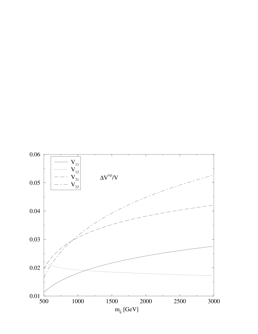
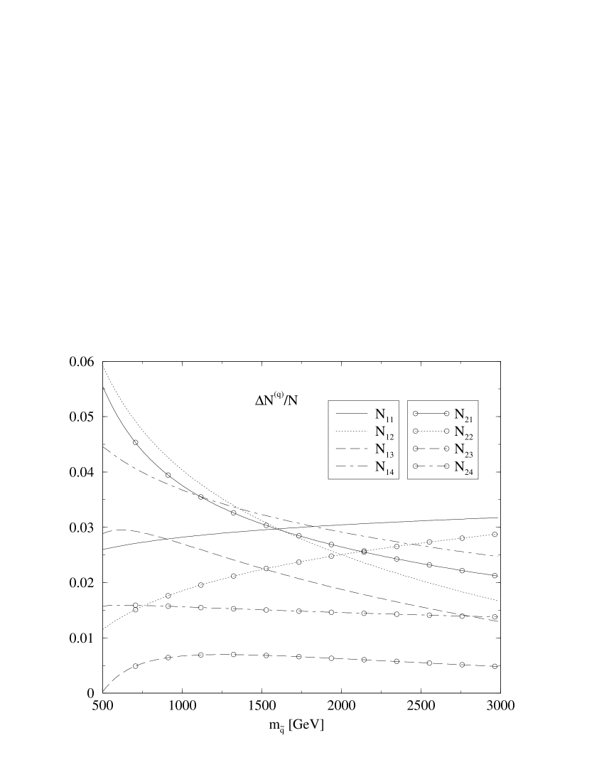
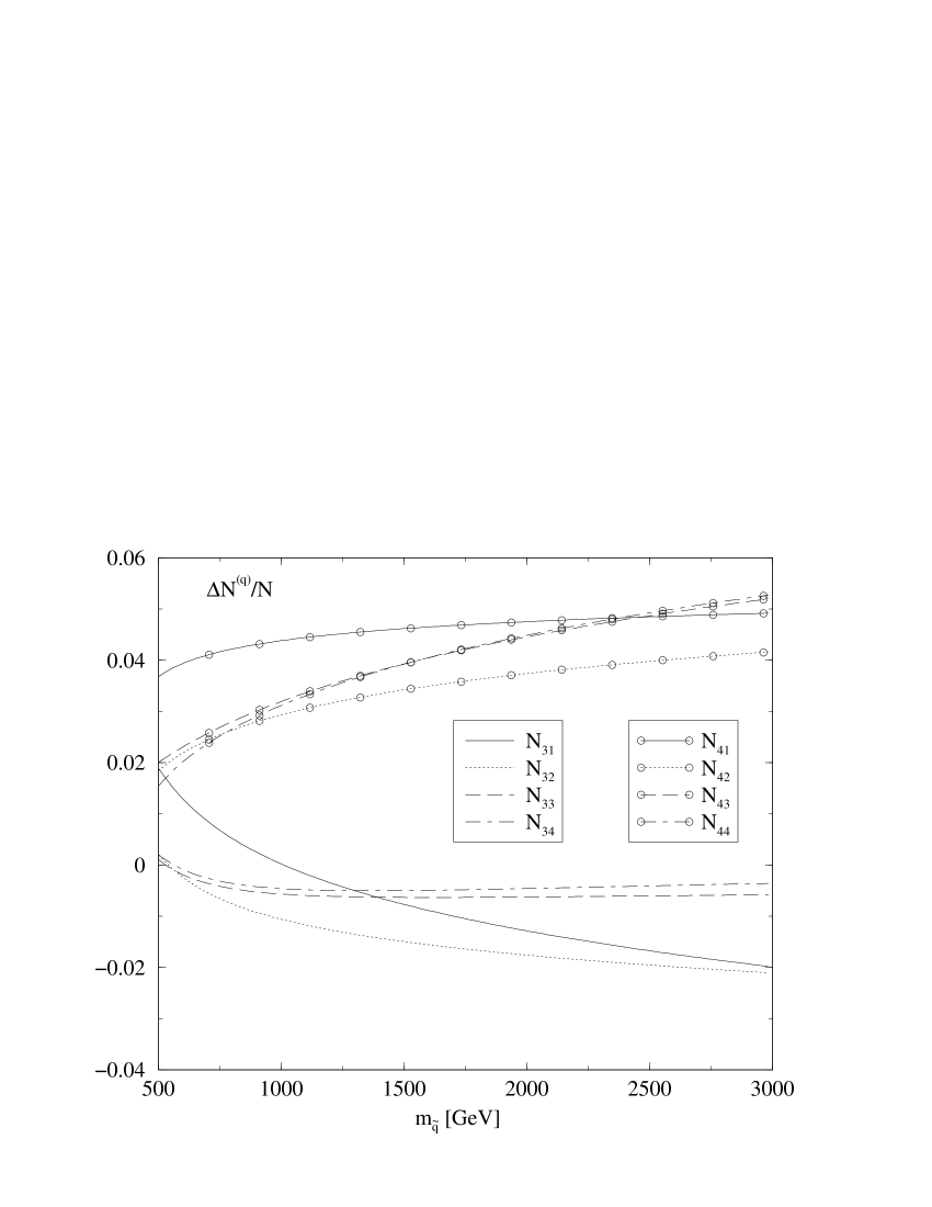
As explained previously these corrections admit a description in terms of effective coupling matrices. In Fig. 6 we show the relative finite shifts induced by the quark-squark sector in the effective coupling matrices as a function of a common soft-SUSY-breaking squark mass parameter. The tree-level values for the mixing matrices are:

$$\begin{array}[]{l}U=\pmatrix{0.91&0.41\cr-0.41&0.91}\,,\\ V=\pmatrix{0.97&0.24\cr-0.24&0.97}\,,\end{array}N=\pmatrix{-0.99&-0.10&-0.06i&0.11\cr 0.06&-0.94&0.09i&-0.32\cr-0.15&0.28&0.69i&-0.64\cr 0.05&-0.16&0.71i&0.68}\,\,.$$ (11)

(a)	(b)
(c)	(d)

Figure 6: Quark-squark contributions to the effective chargino/neutralino mixing coupling matrices (6) as a function of a common squark mass parameter for SPS 1a.

One can perform a one-to-one matching of Fig. 6 with Fig. 5. By neglecting the small electron-higgsino couplings we obtain:

$$\begin{array}[]{rcl}\delta\Gamma^{(q)}(\tilde{e}_{L}\to e^{-}\chi^{0}_{\alpha})/\Gamma&=&2\frac{\Delta N^{(q)}_{\alpha 2}-Y_{L}t_{w}\Delta N^{(q)}_{\alpha 1}}{N_{\alpha 2}-Y_{L}t_{w}N_{\alpha 1}},\\ \delta\Gamma^{(q)}(\tilde{e}_{L}\to\nu_{e}\chi^{-}_{1})/\Gamma&=&2\Delta U^{(q)}_{11}/U_{11},\\ \delta\Gamma^{(q)}(\tilde{e}_{R}\to e^{-}\chi^{0}_{\alpha})/\Gamma&=&2\Delta N^{(q)}_{\alpha 1}/N_{\alpha 1},\\ \end{array}\begin{array}[]{rcl}\delta\Gamma^{(q)}(\tilde{\nu}_{e}\to e^{-}\chi^{+}_{1})/\Gamma&=&2\Delta V^{(q)}_{11}/V_{11},\\ \delta\Gamma^{(q)}(\tilde{\nu}_{e}\to\nu_{e}\chi^{0}_{\alpha})/\Gamma&=&2\frac{\Delta N^{(q)}_{\alpha 2}+Y_{L}t_{w}\Delta N^{(q)}_{\alpha 1}}{N_{\alpha 2}+Y_{L}t_{w}N_{\alpha 1}};\end{array}$$

and $\tilde{e}_{\{L,R\}}=\tilde{e}_{\{1,2\}}$ for the case (10) under study. We see in Fig. 6 variations up to 5% in the coupling matrices, which would translate to variations up to 10% in the observables.

(a)	(b)

Figure 7: Variation of the chargino effective coupling matrices (6) as a function of the top-squark soft-SUSY-breaking trilinear coupling $A_{t}$ for SPS 1a, but with a squark mass scale of 1 TeV.

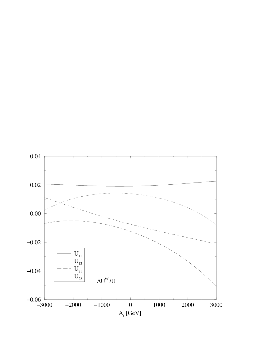
We are also interested in the variation with the soft-SUSY-breaking squark trilinear coupling $A_{q}$. For the first and second generation squarks the variation is negligible. The corrections show some variation with $A_{b}$, but it is well below the 1% level. In Fig. 7 we show the variation of the chargino effective couplings with $A_{t}$. In this figure we have chosen a squark mass scale of 1 TeV. Since $A_{t}$ enters the computation of the physical top-squark masses, choosing a light squark mass scale ($\sim 500\mbox{ GeV}$) would produce light physical top-squark masses ($\sim 100\mbox{ GeV}$) for certain values of $A_{t}$. In that case one would find large variations in the corrections which are due to the presence of light top-squark particles, and not to the trilinear coupling per se. Furthermore, these light top-squark particles could be produced at the LC, and their properties precisely measured. In this figure we see large variations of the corrections (up to 4%), mainly in the higgsino components of the charginos ($U_{i2}$, $V_{i2}$). Therefore these corrections are mainly relevant for the couplings of third generation sfermions ($\tilde{\tau},\tilde{b},\tilde{t}$). Again, a precise knowledge of $A_{t}$ is not necessary to provide a prediction with sufficient precision, but a rough knowledge of the scale and sign is needed.

5 Conclusions

We have computed the complete one-loop EW corrections to the sfermion partial decay widths into charginos and neutralinos. We have combined these corrections with the QCD ones, and provided a combined prediction for these observables. The corrections from the EW sector can be of the same order as that of the QCD sector, therefore both kinds of effects must be taken into account on the same footing.

In these corrections non-decoupling effects appear. These effects are due to two kinds of splittings among the particle masses: a splitting between a particle and its SUSY partner (given by the soft-SUSY-breaking masses); and a splitting among the SUSY particles themselves. In this situation the radiative corrections grow with the logarithm of the largest SUSY particle of the model. In this scenario some of the particles (presumably strongly interacting particles) are heavy, and can only be produced at the LHC, whereas another set of particles (selectrons, lightest charginos/neutralinos) can be studied at the LC, and their properties measured with a precision better than 1%.

In order to provide a prediction at the same level of accuracy, one needs a knowledge of the squark masses (and $A_{t}$) obtained from the LHC measurements, but a high precision measurement of the squark parameters is not necessary.

The effects of squarks can be taken into account by the use of effective coupling matrices in the chargino/neutralino sector. These effects can be extracted from LC data, by finding the finite difference between the mixing matrices obtained from the chargino/neutralino masses, and the mixing matrices obtained from the couplings analysis.

Of course, to reach the high level of accuracy needed at the LC the complete one-loop corrections to the observables under study is needed, but the effective coupling matrices form a necessary and universal subset of these corrections.

Acknowledgments: This collaboration is part of the network “Physics at Colliders” of the European Union under contract HPRN-CT-2000-00149. The work of J.S. has been supported in part by MECYT and FEDER under project FPA2001-3598.

References

- [1] S. Kraml et al., Phys. Lett. B386 (1996) 175, hep-ph/9605412; A. Djouadi, W. Hollik, C. Jünger, Phys. Rev. D55 (1997) 6975, hep-ph/9609419; W. Beenakker et al., Z. Phys. C75 (1997) 349, hep-ph/9610313.
- [2] J. Guasch, W. Hollik, J. Solà, Phys. Lett. B437 (1998) 88, hep-ph/9802329.
- [3] J. Guasch, W. Hollik, J. Solà, Phys. Lett. B510 (2001) 211, hep-ph/0101086; JHEP 0210 (2002) 040, hep-ph/0207364; Nucl. Phys. Proc. Suppl. 116, 301 (2003), hep-ph/0210118.
- [4] J. Guasch, W. Hollik, J. Solà, Radiative Corrections to scalar quark decays in the MSSM, LC-TH-2000-013, hep-ph/0001254.
- [5] M. Böhm, H. Spiesberger, W. Hollik, Fortsch. Phys. 34 (1986) 687; W. Hollik, Fortschr. Phys. 38 (1990) 165.
- [6] P. Chankowski, S. Pokorski, J. Rosiek, Nucl. Phys. B423 (1994) 437, hep-ph/9303309; A. Dabelstein, Z. Phys. C67 (1995) 495, hep-ph/9409375; Nucl. Phys. B 456 (1995) 25, hep-ph/9503443.
- [7] J. M. Frére, D. R. T. Jones, S. Raby, Nucl. Phys. B222 (1983) 11.
- [8] H. Eberl, et al., Phys. Rev. D64 (2001) 115013, hep-ph/0104109. T. Fritzsche, W. Hollik, Eur. Phys. J. C24 (2002) 619, hep-ph/0203159.
- [9] W. Majerotto, hep-ph/0209137.
- [10] T. Hahn, Comput. Phys. Commun. 140 (2001) 418, hep-ph/0012260; T. Hahn, C. Schappacher, Comput. Phys. Commun. 143 (2002) 54, hep-ph/0105349.
- [11] T. Hahn, M. Pérez-Victoria, Comput. Phys. Commun. 118 (1999) 153, hep-ph/9807565; T. Hahn, FeynArts, FormCalc and LoopTools user’s guides, available from http://www.feynarts.de; G. J. van Oldenborgh, Comput. Phys. Commun. 66 (1991) 1.
- [12] Programs to compute the one-loop corrected partial decay width: (sfermion fermion chargino/neutralino) available from http://www-itp.physik.uni-karlsruhe.de/~guasch/progs
- [13] E. Katz, L. Randall, S. Su, Nucl. Phys. B536 (1998) 3, hep-ph/9801416.
- [14] L.J. Hall, R. Rattazzi, U. Sarid, Phys. Rev. D50 (1994) 7048, hep-ph/9306309; M. Carena, et al., Nucl. Phys. B426 (1994) 269, hep-ph/9402253.
- [15] P. Ciafaloni, D. Comelli, Phys. Lett. B446 (1999) 278, hep-ph/9809321; V. S. Fadin, et al., Phys. Rev. D61 (2000) 094002, hep-ph/9910338; M. Beccaria, et al., Phys. Rev. D65 (2002) 093007, hep-ph/0112273.
- [16] M. Carena, et al. Nucl. Phys. B577 (2000) 88, hep-ph/9912516.
- [17] B. C. Allanach et al., in Proc. of the APS/DPF/DPB Summer Study on the Future of Particle Physics (Snowmass 2001) ed. N. Graf, Eur. Phys. J. C 25 (2002) 113 [eConf C010630 (2001) P125] hep-ph/0202233.
- [18] N. Ghodbane, H. U. Martyn, in Proc. of the APS/DPF/DPB Summer Study on the Future of Particle Physics (Snowmass 2001) ed. N. Graf, hep-ph/0201233.