Micro-Canonical Hadron Production in pp collisions

Abstract

We apply a microcanonical statistical model to investigate hadron production in pp collisions. The parameters of the model are the energy $E$ and the volume $V$ of the system, which we determine via fitting the average multiplicity of charged pions, protons and antiprotons in pp collisions at different collision energies. We then make predictions of mean multiplicities and mean transverse momenta of all identified hadrons. Our predictions on nonstrange hadrons are in good agreement with the data, the mean transverse momenta of strange hadron as well. However, the mean multiplicities of strange hadrons are overpredicted. This agrees with canonical and grandcanonical studies, where a strange suppression factor is needed. We also investigate the influence of event-by-event fluctuations of the $E$ parameter.

¹Institute of Particle Physics, Central China Normal University, Wuhan, China
²Institut für Theoretische Physik, J.W.Goethe Universität, Frankfurt am Main, Germany
³Laboratoire SUBATECH, University of Nantes - IN2P3/CNRS - Ecole des Mines de Nantes, Nantes, France

1 Introduction

In pp collisions at high energies a multitude of hadrons is produced. In contradistinction to the pp collisions at low energies even effective theories are not able to provide the matrix elements for these reactions and therefore a calculation of the cross section is beyond the present possibilities of particle physics. In addition, even at moderate energies, many different particles and resonances may be created and therefore the number of different final states becomes huge.

In this situation, statistical approaches may be of great help [1, 2]. It was Hagedorn who noticed that the transverse mass distributions in high energy hadron-hadron collisions show a common slope for all observed particles[3]. This may be interpreted as a strong hint that it is not the individual matrix elements but phase space who governs the reaction. Therefore Hagedorn introduced statistical methods into the strong interaction physics in order to calculate the momentum spectra of the produced particles and the production of strange particles.

Later, after statistical models have been successfully applied to relativistic heavy ion collisions [4, 5, 6, 7, 8, 9, 10, 11], Becattini and Heinz [12] came back to the statistical description of elementary $pp$ and $\bar{p}p$ reactions and used a canonical model (in which the multiplicity of hadrons M is a function of volume and temperature M(V,T)) in order to figure out whether the particle multiplicities predicted by this approach are in agreement with the (in the meantime very detailed) experimental results. For a center of mass energy of around 20 GeV they found for non strange particles a very good agreement between statistical model predictions and data assuming that the particles are produced by a hadronic fireball with a temperature of T = 170 MeV. The strange particles, however, escaped from this systematics being suppressed by factors of the order of two to five. Becattini and Heinz coped with this situation by introducing a $\gamma_{S}$ factor into the partition sum which was adjusted to reproduce best the multiplicity of strange particles as well.

Statistical models are classified according to the implementation of conservation laws:

• microcanonical: both, material conservation laws ($Q,$ $B$, $S,$ $C,$ $\cdots$) and motional conservation laws ($E$, $\overrightarrow{p}$,$\overrightarrow{J}$, $\cdots$), hold exactly.

• canonical: material conservation laws hold exactly, but motional conservation laws hold on average (a temperature is introduced).

• grand-canonical: both material conservation laws and motional conservation laws hold on the average (temperature and chemical potentials introduced).

The intensive physical quantities such as particle density and average transverse momentum are independent of volume in the grand-canonical calculation , while they depend on volume in both canonical and microcanonical calculations. What one naively expects is that the microcanonical ensemble must be used for very small volumes, for intermediate volumes the canonical ensemble should be a good approximation, while for very large volumes the grand-canonical ensemble can be employed. A numerical study of volume effects in paper[14] tells us how big the volumes need to be in order to make the grand-canonical ensembles applicable. The comparison between the microcanonical and the canonical treatment in paper[14] shows a very good agreement in particle yields, when the same volume and energy density are used, and the strangeness suppression is canceled in the canonical calculation.

In this paper, first we ignore the fluctuations of microcanonical parameters and try to fix the microcanonical parameters, energy $E$ and volume $V$, from fitting $4\pi$ yields of protons, antiprotons and charged pions from pp collisions. The one-to-one relation between the collision energy $\sqrt{s}$ and a pair of microcanonical parameters $E$ and $V$ makes a link between the pp experiments and the microcanonical approaches (or more generally, the statistical ensembles). One can easily judge if grand-canonical ensembles can describe pp collisions at any given energy; one can also transform the fitting results to the canonical case and find the corresponding temperature and volume of pp collisions at any energy.

Then we study the effect from the fluctuations of the microcanonical energy parameter at a collision energy of $200\,\mathrm{GeV}$, to check how reliable it is to fix microcanonical parameters without energy fluctuations.

Finally, we would like to make a comparison between statistical models and string models in describing pp collisions. This microcanonical model and this fitting work will provide us a bridge to compare the two classes of models and help us to understand the reaction dynamics. In principle, one can consider a string as an ensemble of fireballs, which may be considered as one effective fireball, when only total multiplicities are considered.

2 The approach

We consider the final state of a proton-proton collision as a “cluster” , “droplet” or “fireball” characterized by its volume $V$ (the sum of individual proper volumes), its energy $E$ (the sum of all the cluster masses) and the net flavour content $Q=(N_{u}-N_{\bar{u}},N_{d}-N_{\bar{d}},N_{s}-N_{\bar{s}})$, decaying “statistically” according to phase space. More precisely, the probability of a cluster to hadronize into a configuration $K=\{h_{1},p_{1};\ldots;h_{n},p_{n}\}$ of hadrons $h_{i}$ with four momenta $p_{i}$ is given by the micro-canonical partition function $\Omega(K)$ of an ideal, relativistic gas of the $n$ hadrons [13],

$$\Omega(K)=\frac{V^{n}}{(2\pi\hbar)^{3n}}\,\prod_{i=1}^{n}g_{i}\,\prod_{\alpha\in\mathcal{S}}\,\frac{1}{n_{\alpha}!}\,\prod_{i=1}^{n}d^{3}p_{i}\,\delta(E-\Sigma\varepsilon_{i})\,\delta(\Sigma\vec{p}_{i})\,\delta_{Q,\Sigma q_{i}},$$

with $\varepsilon_{i}=\sqrt{m_{i}^{2}+p_{i}^{2}}$ being the energy, and $\vec{p}_{i}$ the 3-momentum of particle $i$. The term $\delta_{Q,\Sigma q_{i}}$ ensures flavour conservation; $q_{i}$ is the flavour vector of hadron $i$. The symbol $\mathcal{S}$ represents the set of hadron species considered: we take $\mathcal{S}$ to contain the pseudoscalar and vector mesons $(\pi,K,\eta,\eta^{\prime},\rho,K^{*},\omega,\phi)$ and the lowest spin-$\frac{1}{2}$ and spin-$\frac{3}{2}$ baryons $(N,\Lambda,\Sigma,\Xi,\Delta,\Sigma^{*},\Xi^{*},\Omega)$ and the corresponding antibaryons. $n_{\alpha}$ is the number of hadrons of species $\alpha$, and $g_{i}$ is the degeneracy of particle $i$. We generate randomly configurations $K$ according to the probability distribution $\Omega(K)$. For the details see ref. [13]. The Monte Carlo technique allows to calculate mean values of observables as

$$\bar{A}=\sum_{K}A(K)\,\Omega(K)/\sum_{K^{\prime}}\Omega(K^{\prime}),$$

where $\sum$ means summation over all possible configurations and integration over the $p_{i}$ variables. $A(K)$ is some observable assigned to each configuration, as for example the number $M_{h}(K)$ of hadrons of species $h$ present in $K$. Since $\bar{A}$ depends on $E$ and $V$, we usually write $\bar{A}(E,V)$. $Q$ is not mentioned, since we only study $pp$ scattering here, therefore $Q$ is always $(4,2,0)$.

Let us consider the hadron multiplicity $\bar{M}_{h}(E,V)$. This quantity is used to determine the energy $E(\sqrt{s})$ and the volume $V(\sqrt{s})$ which reproduces best the measured multiplicity of some selected hadrons in pp collisions at a given $\sqrt{s}$ . This is achieved by minimizing $\chi^{2}$:

$$\chi^{2}(E,V)=\frac{1}{\alpha}\sum_{j=1}^{\alpha}\frac{[\bar{M}_{\mathrm{exp},j}(\sqrt{s})-\bar{M}_{j}(E,V)]^{2}}{\sigma_{j}^{2}}$$

where $\bar{M}_{\mathrm{exp},j}(\sqrt{s})$ and $\sigma_{j}$ are the experimentally measured multiplicity and its error of the particle species $j$ in pp collisions at an energy of $\sqrt{s}$.

We start out our investigation by taking as input the most copiously produced particles ($j=p,\bar{p},\pi^{+},\pi^{-}$). The data have been taken from [15]. Whenever the data are not available, the extrapolation of multiplicities by Antinucci [15] is used. Fig.1 displays the results of our fit procedure in comparison with the experimental data. We observe that these 4 particle species can be quite well described by a common value of $E(\sqrt{s})$ and $V(\sqrt{s})$.

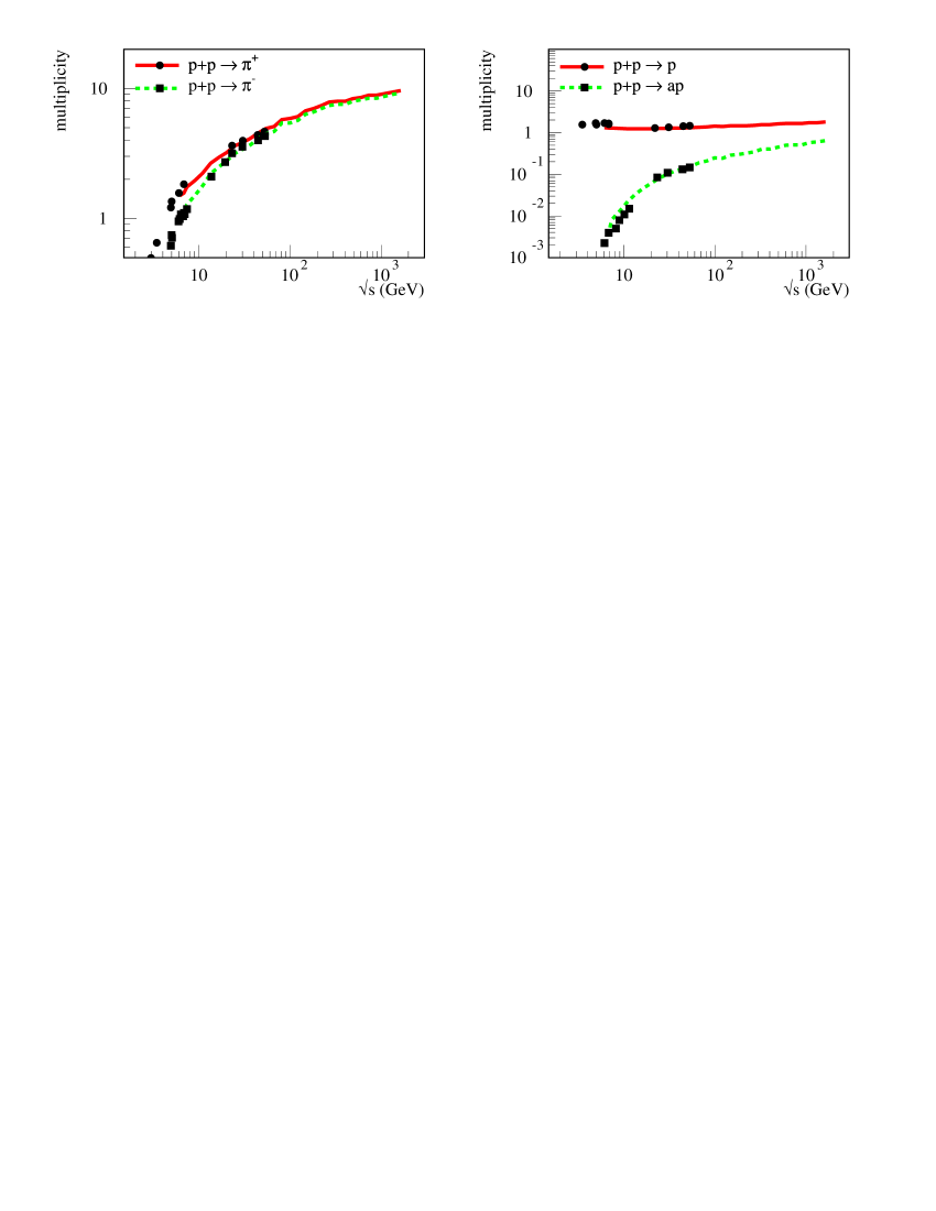
Figure 1: The 4$\pi$ multiplicities of $\pi^{+},\pi^{+}$, proton, antiproton produced in a pp collision as a function of $\sqrt{s}$. The full and dashed lines show the result of the $\chi^{2}$ fit. The points are data from [15].

Fig.2 shows $E(\sqrt{s})$ and $V(\sqrt{s})$, and fig.3 the energy density $\epsilon(\sqrt{s})=E(\sqrt{s})/V(\sqrt{s})$, which we obtain as the result of our fit. Both energy and volume increase with $\sqrt{s}$ but rather different, as the energy density shows. We parameterize the energy and volume dependence on the collision energy $\sqrt{s}$ in eq. (1).

$$E/\mathrm{G}eV = -3.8+3.76\mathrm{ln}\sqrt{s}+6.4/\sqrt{s}$$

$$V/\mathrm{f}m^{3} = -30.0376+14.93\mathrm{ln}\sqrt{s}-0.013\sqrt{s}$$ (1)

where $\sqrt{s}$ is in unit GeV. Below $\sqrt{s}$ = 8 GeV the fit produces volumes below 2fm³ which cannot be interpreted physically. Above $\sqrt{s}$ = 8 GeV the volume increases very fast as compared to the energy giving rise to a decrease in the energy density until - around $\sqrt{s}$ = 200 GeV - the expected saturation sets in and the energy density becomes constant. In view of the large volume observed for these large energies the density of the different particles does not change anymore [14] and therefore the particle ratios stay constant above this energy.

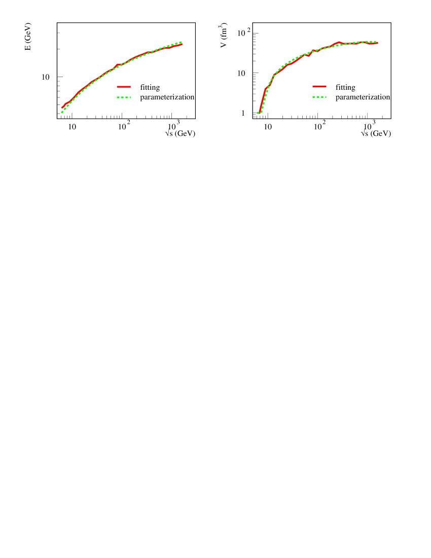
Figure 2: The dependence of micro-canonical parameters $E$ (left) and volume $V$ (right) on the collision energy $\sqrt{s}$ . The parameterization described as eq. (1) is plotted as dashed lines.

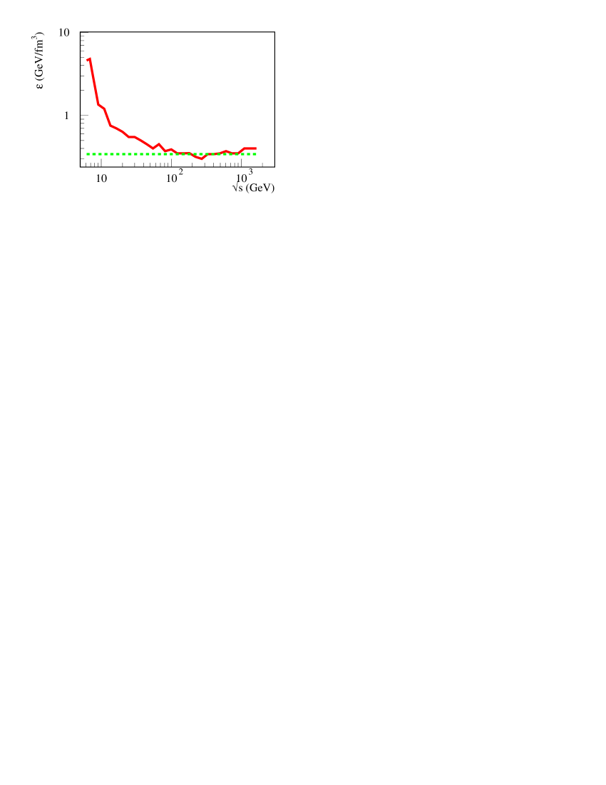
Figure 3: The dependence of energy density $\varepsilon=E/V$ on the collision energy $\sqrt{s}$. The dashed line corresponds to constant energy density $0.342\,\mathrm{G}eV/\mathrm{f}m^{3}$ which comes from a canonical calculation[12, 14].

The quality of the fit can be judged from fig.4 where we have plotted the $\chi^{2}$ values obtained for different values of $E$ and $V$ and for $\sqrt{s}$ = 200 GeV. We see that the energy variation is quite small whereas the volume varies more. Nevertheless the energy density is rather well defined.

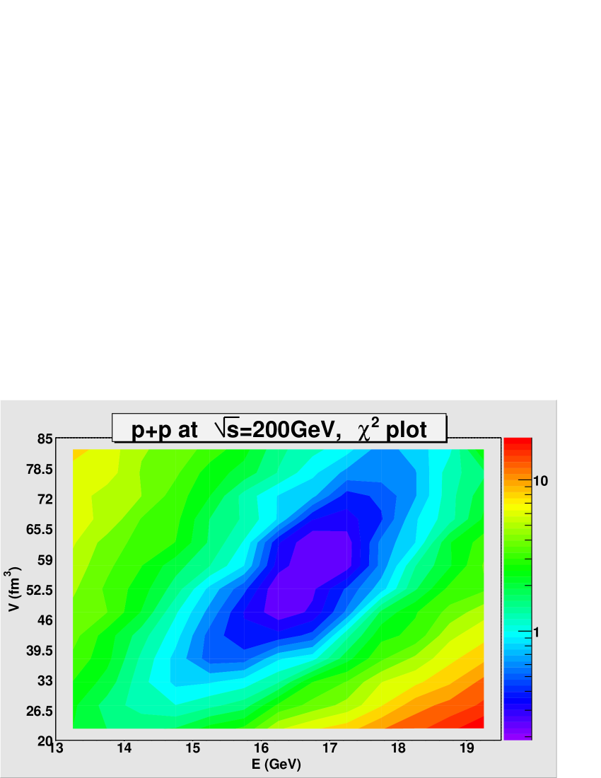
Figure 4: The value of $\chi^{2}$ for different values of $E$ and $V$ for a pp reaction at $\sqrt{s}=200\,\mathrm{GeV}$.

After having fitted the $E(\sqrt{s})$ and $V(\sqrt{s})$ in using $p,\bar{p},\pi^{+}$ and $\pi^{-}$ data we can now use these fitted values to predict the multiplicity of other hadrons. This study we start in Fig. 5, where we present the multiplicity of $\pi^{0}$ and $\rho^{0}$. For these particles experimental data are available. We see that the absolute value as well as the trend of the experimental data is quite well reproduced. The result for those hadrons, for which no or only few data are available, is displayed in fig. 6. As one can see the overall agreement is remarkable. We would like to mention that we have as well made a $\chi^{2}$ fit using as input the measured multiplicities of $p,\bar{p}$ and $\rho^{0}$. The results for $E(\sqrt{s})$ and $V(\sqrt{s})$ differ only marginally.

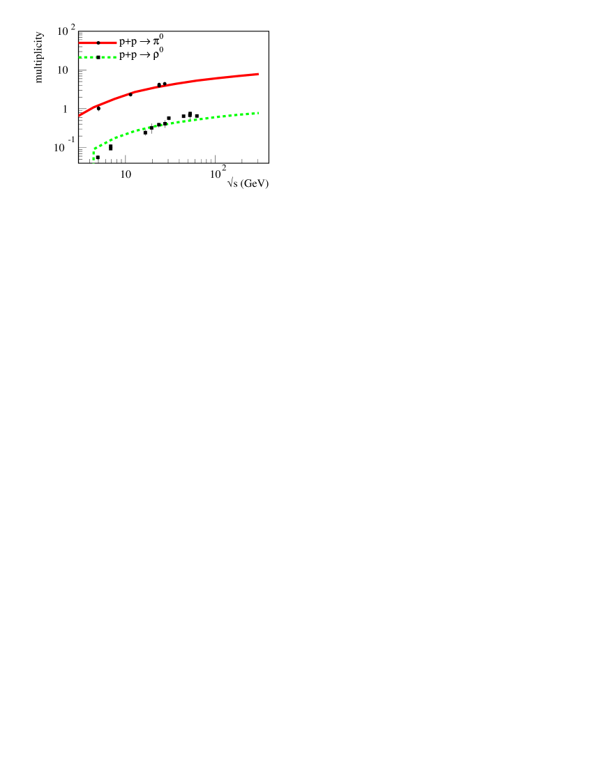
Figure 5: Prediction of the $\pi^{0}$and $\rho^{0}$ multiplicity in pp collisions as a function of $\sqrt{s}$. The result of the calculation is compared to the data [16].

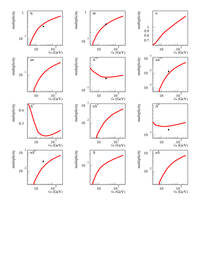
Figure 6: Predictions of the multiplicities of non strange hadrons in pp collisions as a function of $\sqrt{s}$. We have plotted, if available, also the data points for $\sqrt{s}=27.5\,\mathrm{GeV}$ [17]

3 Strange particles

With the parameters $E(\sqrt{s})$ and $V(\sqrt{s})$ which we have obtained from the fit of the $p,\,\bar{p},\,\pi^{+}$ and $\pi^{-}$ multiplicities, we can as well calculate the multiplicity of strange particles or particles with hidden strangeness. The results of these fits are presented in Fig. 7. As we can see immediately the results for those particles are not at all in agreement with the data. $\Lambda$ and $\phi$ multiplicities are off by a factor of 3-5 roughly, for the $\bar{\Lambda}$ the situation may be similar but the spread of the experimental data does not allow for a conclusion yet. Only the kaons come closer to the experimental values. Although at lower energies a part of this deviation may come from the fact that in our Monte Carlo procedure weak decays are neglected and therefore $K^{0}$ and $\bar{K}^{0}$ are the particle states which are treated, at higher energies this is not of concern anymore. At $\sqrt{s}=53\,\mathrm{GeV}$, we find - as in experiment - that $K_{L}=K_{S}$ and hence $K^{0}=\bar{K}^{0}$. Therefore, as in experiment, one finds that the strangeness contained in $\Lambda,\,\bar{\Lambda},\,K^{+}$ and $K^{-}$ adds up to zero. The absolute numbers are, however, rather different: experimentally one finds .41 $K^{+}$, 0.29 $K^{-}$ and 0.12 $\Lambda$ [18, 19], whereas the fit yields 1.16 $K^{+}$, 0.66 $K^{-}$ and 0.58 $\Lambda$.

One is tempted to try to fit the strange particles separately. The result at large $\sqrt{s}$ is that, in contradiction to experiment, more $K^{0}$ then $\bar{K}^{0}$ are produced. Consequently, the strangeness in $\Lambda,\,\bar{\Lambda},\,K^{+}$ and $K^{-}$ does not add up to zero and the fit is far away from the data. Thus we have to conclude that the strange particle multiplicities cannot be described in a phase space approach using the parameters one obtains from the fit of non strange particles, and that there is no understanding presently why the suppression factor is rather different for the different hadrons.

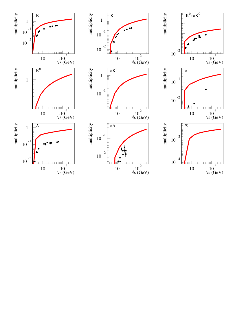
Figure 7: Prediction of the multiplicity of strange hadrons in pp collisions as a function of $\sqrt{s}$. The result of the calculation is compared to the data [16].

As mentioned above, in the past there has been proposed to use an additional parameter, $\gamma_{s}$, in order to describe the strangeness suppression. This parameter has been interpreted as a hint that the volume in which strangeness neutrality has to be guaranteed is small as compared to the volume of the system. However, a detailed comparison of the multiplicity of all strange particles with the data shows [12] that one additional parameter alone is not sufficient to describe the measured multiplicities of the different strange particles in a phase space approach to pp collisions.

4 Transverse Momenta

Phase space calculations predict not only particle multiplicities but also the momenta of the produced particles. The average transverse momenta of the produced particle give a good check whether the energy density obtained in the fit can really be interpreted as the energy density of a hadron gas. Fig. 8 shows the average transverse momenta in comparison with the experimental data [18]. We see that over the whole range of beam energies the average transverse momenta are in good agreement with the data. This confirms that the partition of the available energy into energy for particle production and kinetic energy is correctly reproduced in the phase space calculation. It is remarkable that the average transverse momenta of strange particles is correctly predicted.

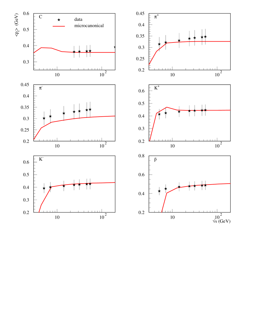
Figure 8: Average transverse momenta as predicted in the phase space calculation as a function of $\sqrt{s}$ in comparison with the experimental values [18] for different particle species.

5 Energy Fluctuations

Up to now we have assumed that for a given center of mass energy, the energy of the droplet $E$ has an unique value, given in fig. 2. This is of course not a realistic assumption. Most probably the energy varies from event to event but little is known about the form of this fluctuation. The only quantity for which data are available is the multiplicity distribution of charged particles, which has been the subject of an extensive discussion in the seventies due to the finding of a scaling law, called KNO scaling. Of course, one can try now to find an energy distribution which yields the experimental charge particle distribution but this relation is not unique and therefore little may be learnt.

It has also been suggested to replace the microcanonical ensemble calculation, presented here, in favor of a canonical ensemble or an ensemble where the pressure is the control parameter, however it is difficult to find a convincing argument. It is the dynamics of the reaction which determines which fraction of the energy goes into collective motion, and which fraction into particle production. This has nothing to do with a heat bath nor with constant pressure on the droplet. Consequently, the relation between the energy fluctuation, seen in a system with a fixed temperature, and the true energy fluctuation is all but evident.

Therefore, we use another approach to study the influence of energy fluctuations on the observables. We assume that the volume of the system remains unchanged in order not to have too many variables and that the energy fluctuates. For technical reasons, we use discrete distributions, using $E_{i}=i\,\Delta E$, with $\Delta E=1$GeV. For $\sqrt{s}=200\,\mathrm{GeV}$, we have $\left\langle E\right\rangle=16.15\,\mathrm{GeV}$ from the above fitting work, and correspondingly we take $<i>=16.15$. We study three cases:
a) The energy distribution is Poissonian

$$\mathrm{Prob}(i)=\frac{\left\langle i\right\rangle^{i}\mathrm{exp}(-\left\langle i\right\rangle)}{i!}$$

and
b) The energy distribution is Gaussian

$$\mathrm{Prob}(i)=\left\{\begin{array}[]{c}\frac{1}{0.63}\frac{1}{\sqrt{2\pi}\sigma}\mathrm{exp}(-\frac{E_{i}-\mu}{\sigma})^{2}\,\,\,\,\mathrm{when}\,E_{i}\in[2.5\,\mathrm{GeV},\infty)\\ 0\,\,\,\,\,\,\,\,\,\,\,\,\,\,\,\,\,\,\,\,\mathrm{otherwise}.\end{array}\right.$$

where an energy threshold of $2.5\,\mathrm{GeV}$ is taken for the proton-proton system. $\mu=\sigma=14.01\mathrm{GeV}$ to obtain $\left\langle i\right\rangle=16.15$ and the factor 0.63 is used to normalize the energy distribution, and
c) The energy distribution is a negative binomial distribution

$$P^{\mathrm{NB}}(i;\,n,k)=\frac{k(k+1)\cdots(k+i-1)}{i!}\frac{n^{i}k^{k}}{(n+k)^{n+k}}.$$

The negative binomial distribution is well normalized, and $<i>=n$. So we take $n=16.15$. The parameter $k=3$ is chosen to get the best fit to multiplicity distribution data from UA5.

All the three types of energy fluctuations are displayed in fig. 9.

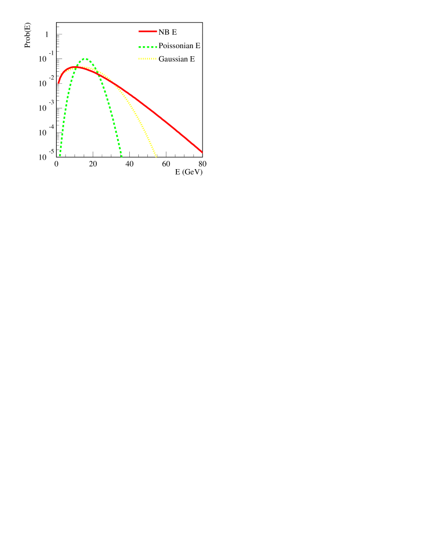
Figure 9: The Gaussian, Poissonian and the NB energy fluctuations.

In Fig. 10, we display the influence of these fluctuations on the charged hadron multiplicity distributions. We compare the results from a fixed energy of 16.15 GeV, the energy with a fluctuation of the above-mentioned Poissonian, Gaussian and the NB type. We see that already for a fixed energy the fluctuation of the charged particle multiplicity is considerable. Different energy fluctuations give different multiplicity distributions. The NB energy fluctuation reproduces the UA5 data for non single diffractive events in antiproton-proton collisions at $\sqrt{s}=200\mathrm{GeV}$.

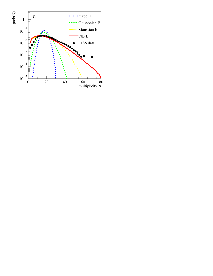
Figure 10: Distribution of the multiplicity of charged hadrons. We display the results from a fixed energy of 16.15 GeV, the energy with a distribution of the above-mentioned Poissonian, Gaussian and the 2-NB type. Also displayed are the UA5 data for non single diffractive events[20].

How does the multiplicity of identified hadrons fluctuate if the droplet energy fluctuates? This is studied in fig. 11, where we display the multiplicity distribution of the most copiously produced particles for fixed energy $E=16.15\,\,\mathrm{GeV}$ and for a Poissonian, Gaussian and NB energy distribution. We see here as well that already for a fixed droplet energy the multiplicity fluctuations are important. Though different energy fluctuations cause different multiplicity distribution, the energy fluctuation gives very little effect in the average multiplicities. So our approach, fixing microcanonical parameters by fitting the averager multiplicity data, is quite reliable.

There is also a correlation between the pion and kaon multiplicity in a given event, shown in table.1. The event averaged K/$\pi$ ratio is considerably different from the ratio of the average kaon and the pion multiplicity. The energy fluctuations change more the event averaged K/$\pi$ ratio than the ratio of the average kaon and the pion multiplicity.

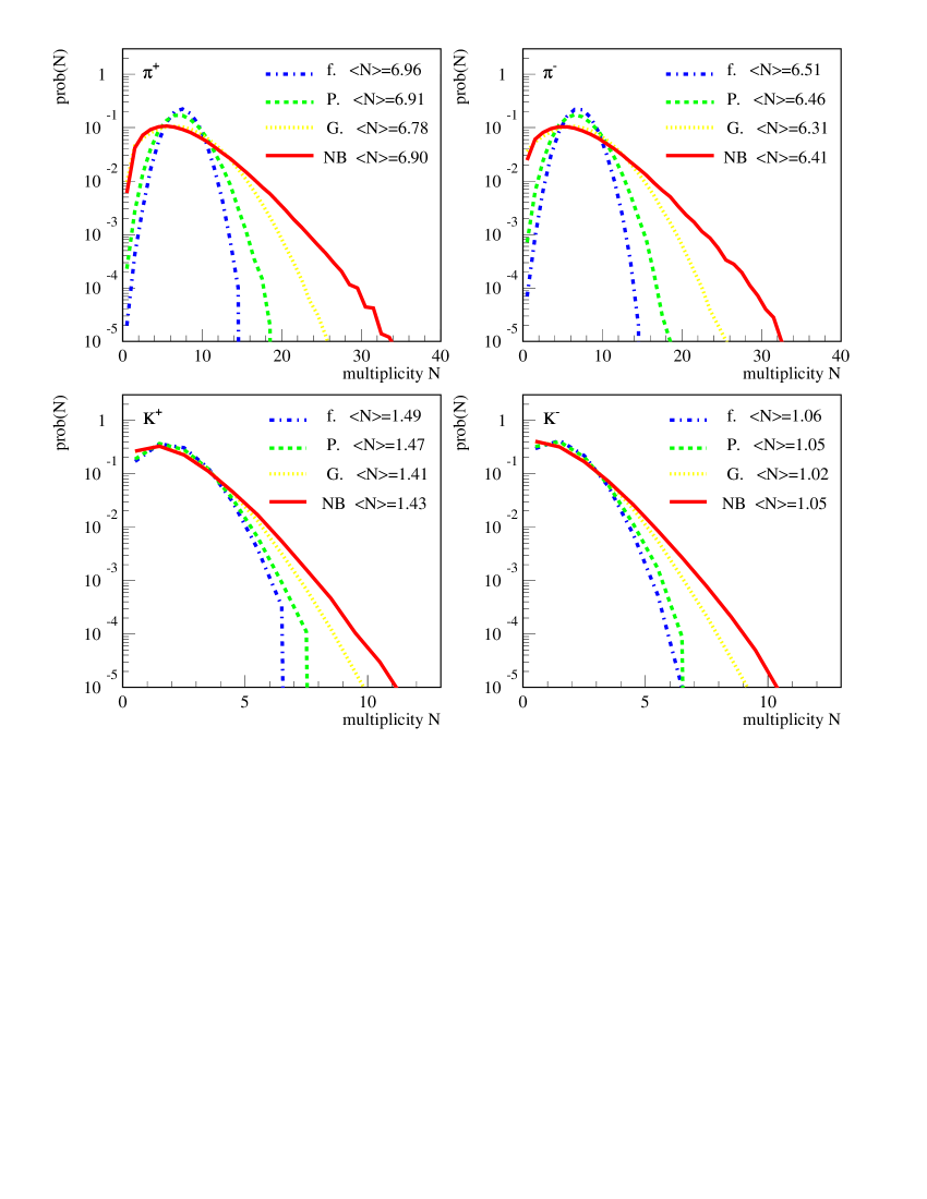
Figure 11: Multiplicity distribution of charged pions and kaons from a fixed energy of 16.15 GeV, the energy with a distribution of the above-mentioned Poissonian, Gaussian and the NB. The number refers to the mean multiplicity.

	$\frac{\left\langle K^{+}\right\rangle}{\left\langle\pi^{+}\right\rangle}$	$\frac{\left\langle K^{-}\right\rangle}{\left\langle\pi^{-}\right\rangle}$	$\left\langle\frac{K^{+}}{\pi^{+}}\right\rangle$	$\left\langle\frac{K^{-}}{\pi^{-}}\right\rangle$
fixed E	0.214	0.163	0.253	0.197
Poissonian E dis.	0.213	0.163	0.251	0.194
Gaussian E dis.	0.208	0.162	0.241	0.179
NB E dis.	0.208	0.163	0.241	0.180

Table 1: Different K to $\pi$ ratios where $\left\langle...\right\rangle$ means event averaging.

6 Conclusion

We have presented a micro-canonical phase space calculation to obtain particle multiplicities and average transverse momenta of particles produced in pp collisions as a function of $\sqrt{s}$. Using the multiplicities of $p,\,\bar{p},\,\pi^{+},\,\pi^{-}$, we fit the two parameters of the phase space approach, the volume and the energy.

Using these two parameters, we calculate the multiplicities of all the other hadrons as well as their average transverse momenta. The calculated multiplicities agree quite well with experiment as far as non strange hadrons are concerned.

For the yields of strange hadrons (as well as those with hidden strangeness), the prediction is off by large factors. In canonical and grand-canonical approaches, strangeness suppression factor have been used to solve this problem.

The energy obtained by this fit is much smaller than the energy available in the center of mass system of the pp reaction, because part of the energy goes into collective motion in beam direction. Nevertheless, the average transverse momenta of the produced particles (not only non-strange but also strange) from this fitting agree quite well with experiment.

We learn that the volume of the pp collision system increases with the collision energy. However, it saturates at very high energy(with Antinnuci’s parameterization as input). The maximum value does not exceed $100\,\mathrm{fm}^{3}$. Together with the results from article [14], we conclude that the grand-canonical treatment cannot describe particle production in pp collisions even at high energy.

We study the effects from energy fluctuations and find that it is quite reliable to fix the microcanonical parameters without considering energy fluctuations.

Acknowledgement

F.M.L would like to thank H. Stöcker and the theory group in Frankfurt for the kind hospitality and F. Becattini for many helpful discussions.

References

- [1] E. Fermi, Prog. Theor. Phys. 5, 570 (1950); Phys.Rev. 81 (1951) 683.
- [2] L. D. Landau, Lzv. Akd. Nauk SSSR 17 (1953) 51; Collected papers of L. D. Landau, ed. D. Ter Haar, Gordon and Breach, New York, 1965
-
[3]
R. Hagedorn, Supplemento al Nuovo Cimento, 3 (1965) 147.
R. Hagedorn and J. Randt, Supplemento al Nuovo Cimento, 6 (1968) 169.
R. Hagedorn, Supplemento al Nuovo Cimento, 6 (1968) 311. - [4] R. Hagedorn, Nucl. Phys. B 24 (1970) 93.
- [5] P. Siemens, J. Kapusta, Phys. Rev. Lett. 43 (1979) 1486.
- [6] A. Z. Mekjian, Nucl. Phys. A384 (1982) 492.
- [7] L. Csernai, J. Kapusta Phys. Rep. 131 (1986) 223.
- [8] H. Stoecker, W. Greiner, Phys. Rep. 137 (1986) 279.
- [9] J. Cleymanns and H. Satz, Z. Phys. C57 (1993) 135; J. Cleymanns, D. Elliott, H. Satz, and R.L. Thews, CERN-TH-95-298, (1996).
- [10] J. Rafelski and J. Letessier, J. Phys. G: Nucl. Part. Phys. 28 (2002) 1819-1832.
- [11] P. Braun-Munzinger, K. Redlich and J. Stachel, arXiv:nucl-th/0304013.
- [12] F. Becattini and U. Heinz Z.Phys. C76 (1997) 269.
- [13] K. Werner and J. Aichelin, Phys. Rev. C52 (1995) 1584-1603
- [14] F.M. Liu, K. Werner, J. Aichelin, hep-ph/0304174, Phys. Rev. C 68 (2003) 024905.
-
[15]
M. Antinucci et al., Lett. Nuov. Cim., V6, N4,(1973) 27.
G. Giacomelli, Phys. Rep. 23C (1976) 123. - [16] D. Drijard et al., Z. Phys. C9 (1981) 293.
- [17] M. Aiguilar-Benitez et al., Z. Phys. C50 (1991) 405.
- [18] R.E. Rossi et al. Nucl. Phys. B84 (1975) 269.
- [19] Erhan et al. Phys. Lett. 85B (1979) 447.
- [20] UA5 Collaboration, R.E. Ansorge et al., Z.Phys.C43:357,1989.