hep-ph/0307004

Spontaneous and dynamical symmetry breaking in higher-dimensional space-time with boundary terms

Hiroyuki Abe

Department of Physics, Korea Advanced Institute of Science and Technology,
Daejeon 305-701, Korea

Doctoral thesis submitted to

Department of Physics, Hiroshima University

18 February 2003

In this thesis we study physics beyond the standard model focusing on the quantum field theory in higher-dimensional space-time with some boundary terms. The boundary term causes nontrivial consequences about the vacuum structure of the higher-dimensional theory. We take particular note of two independent solutions to the weak and Planck hierarchy problem: “low scale supersymmetry” and “dynamical electroweak symmetry breaking.” From a viewpoint of the low scale supersymmetry, we study $F$ and $D$ term supersymmetry breaking effects on sparticle spectra from a boundary. While we also investigate a nonperturbative effect caused by a bulk (nonsupersymmetric) gauge dynamics on a fermion bilinear condensation on a boundary, and analyze the dynamical symmetry breaking on the brane. From these analyses we conclude that the field localization in higher-dimensional space-time involves in a nontrivial vacuum structure of the theory, and the resultant low energy four-dimensional effective theory has phenomenologically interesting structure. In a framework of purely four-dimensional theory, we also construct the above nontrivial effect of localization in the extra dimension.

Chapter 1 Our world as a boundary plane

The unification of all forces and matters in our world within a single theory is most important and challenging issue in modern theoretical particle physics. We have a quantum gauge field theory (QGFT) called standard model (SM) with the gauge group $SU(3)_{c}\times SU(2)_{W}\times U(1)_{Y}$ that describes strong and electroweak interaction between matter particles, that is quarks and leptons. All of the experimental results done till now assures the validity of SM. In a theoretical sense, however, SM has some serious problems. One of them is that it has so many free parameters which must be given from experimental results. For example quark and lepton masses and mixing angles are not predicted from SM itself. Almost all these parameters are related to the Higgs sector which induces electroweak symmetry breaking $SU(2)_{W}$ $\times$ $U(1)_{Y}$ $\to$ $U(1)_{EM}$. Even if we embed SM into the grand unification theory (GUT) such as $SU(5)$, $SO(10)$ and $E_{6}$, the GUT Higgs sectors also have many degrees of freedom and results in the same situation as SM. Therefore we should illuminate the origin of Higgs fields and the mechanism of spontaneous (dynamical) symmetry breaking in SM and GUT.

SM also has a severe difficulty that it doesn’t include gravity although we never doubt its existence because it is a most familiar force in our life. Gravity is in a sense very fundamental force because it originates from the structure of space-time as is insisted in general relativity and couples to all particles universally. If gravity has the same ultimate origin as the SM forces, it should be described by the quantum theory. But QGFT can not treat the gravity ably because of its nonrenormalizable nature. The most successful and interesting candidate of the quantum theory of gravity is string theory. String theory gives not only quantum gravity but also QGFT that means that it may include SM within itself. Unfortunately we can not explicitly show in a present stage that string theory gives us SM uniquely because it has huge number of various degenerate vacuum like or unlike SM.

When we consider the unification of the SM forces and the gravity, we also have a hierarchy problem between the electroweak scale ${\cal O}(10^{2})$ GeV and the Planck scale ${\cal O}(10^{18})$ GeV. This is elegantly solved by introducing supersymmetry (SUSY) at the electroweak scale. But we have so many extra field in addition to the SM contents that we have another difficulty: how to realize SUSY breaking (dynamically) without conflicting experimental results. So the realistic SUSY breaking or the other mechanism which solves the hierarchy problem should be included in such a ultimate unification theory like the string theory.

Taking above situations into account there are two kinds of positions for us to take to study the unification of SM and gravity. One is to improve string theory itself by extending it to, e.g., string field theory, M-theory, matrix model in order to determine the real vacuum that is expected to give SM in four-dimensional space-time. The other is to improve SM side for the purpose to find what kind of improvement resolves the problems in SM and likely leads it to the unification with gravity. In this thesis we stand on the latter stance. In usual bottom-to-up approaches for improving SM, we add new symmetry, new fields, and so on, in four-dimensional space-time. We should consider the origin of such new things when they are added. Our clue for studying beyond the SM is a fact that the known theories of quantum gravity such as supergravity or string theory are consistently defined in more than four-dimensional space-time. The extra dimensions should be hided somehow to give SM in four-dimensional space-time as an low energy effective theory near the electroweak scale. Inversely we should say that there is a possibility to have extra dimensions above the electroweak scale.

Most common idea to yield four-dimensional space-time is to compactify extra dimensions so as not to appear in low energy world. Theories in higher-dimensional space-time with compact extra dimension generically have extra fields called moduli fields in terms of the four-dimensional viewpoint. For example, the extra dimensional components of the gravity or vector (gauge) fields looks like scalar fields in effective four-dimensional theory. These are the candidate for the Higgs fields that induces various symmetry breaking in the four-dimensional world.

However recent discovery of D-branes [1] in string theory gives new aspects to such hiding mechanism. D-brane is a solitonic object on which the open string endpoint terminates. The idea is that our four-dimensional world is realized on a boundary plane in higher dimensional space-time. We consider that our standard model matter particles are confined on a four-dimensional boundary. Such a picture gives many solutions of SM puzzles. One of the remarkable target is weak and Planck hierarchy problem mentioned above. If the number of space-time dimension that gravity propagates is lager than one of SM, our gravity scale, namely, four-dimensional Planck scale is suppressed by the volume of the extra space [2, 3]. There are some explicit models realizing SM gauge group and chiral matter contents directly based on such string models with D-branes, e.g., by intersecting D-branes [4]. Some of these models can obtain weak and Planck hierarchy by such volume suppression mechanism. Of course domain walls in QGFT that is known before the discovery of D-brane is another candidate for such boundary plane. The formation of domain walls is deeply related to the spontaneous symmetry breaking.

Then we are going to be interested in how to solve problems in SM by assuming it to be in the higher-dimensional space-time with such boundaries. Because almost all the ambiguities in QGFT (SM) originate from the sectors (e.g., Higgs sector or hidden sector for SUSY breaking) where spontaneous symmetry breaking occurs, first of all we should pay attention to such sectors. In this thesis we investigate spontaneous and dynamical symmetry breaking in quantum field theory in higher-dimensional space-time with some boundary terms, e.g. boundary matter field. In the theories of unification there are kinds of symmetries that should be broken spontaneously (dynamically) like electroweak symmetry, grand unification symmetry and SUSY.

First we consider the SUSY gauge theories in higher-dimensional space-time with boundaries. Such models can give some realistic SUSY breaking and its mediation mechanisms. In usual scenario in four-dimension, it is sometimes unnatural that we don’t have tree-level direct couplings between SUSY breaking (hidden) sector and SM (visible) sector. In the bulk and boundary system with extra dimensions, we can sequester a hidden sector (brane) from a visible sector (brane) by spatiality of extra dimension. Some interesting mechanisms of SUSY breaking communication are proposed in extra dimension such as gaugino, Kaluza-Klein and radion mediated scenario. We will briefly review them in Chapter 2. These SUSY breaking contributions are based on the $F$ term breaking in some hidden supermultiplet. As in the case of Froggatt-Nielsen mechanism [5] for realistic Yukawa couplings, if the gauge group includes $U(1)$ symmetry, we generally have tadpoles of auxiliary field in the vector multiplet on the four-dimensional boundaries. These tadpoles induce $D$ term SUSY breaking contributions by the well-known way called Fayet-Iliopoulos mechanism. We will also analyze SUSY breaking structure in the bulk with such contributions in Chapter 3.

Next we treat the dynamical chiral symmetry breaking via fermion bilinear condensation, that is a basis for studying dynamical breaking of symmetry without large ambiguities like a scalar potential. The electroweak symmetry is in a sense gauged chiral symmetry, and SUSY breaking through gaugino condensation is similar to the situation of fermion bilinear condensation in dynamical chiral symmetry breaking. We are motivated by analyzing such symmetry breaking in higher-dimensional space-time with boundary terms. In Chapter 4 we will review scenarios of dynamical electroweak symmetry breaking through fermion bilinear condensation that is another mechanism to stabilize weak and Planck hierarchy without low energy SUSY. First we formulate the 4D effective Lagrangian of the gauge theory in the bulk and boundary system in Chapter 5. The most simple way to study dynamical symmetry breaking via fermion bilinear condensation is to use four-fermion approximation and follows the way by Nambu-Jona-Lasinio (NJL) [6]. In chapter 6 we will analyze models with such a four-fermion interaction induced on a brane, and also the interaction which mix a bulk and a brane fermion, and obtain chiral phase structure in terms of the bulk configuration. We also take the gauge boson propagating effect into account by using improved ladder Schwinger-Dyson (SD) equation technique [7] and have nontrivial properties of dynamical fermion mass as a result in Chapter 7. We conclude that the dynamical symmetry breaking in higher-dimensional space-time with boundary terms has rather rich structure compared with the usual four-dimensional one.

In Chapter 8 we consider the theory with product gauge group defined in four-dimensional space-time, which possesses higher-dimensional nature. This gives the new aspects on the difficulties in SM in terms of the higher-dimensional theories, but just in four-dimensional space-time. Finally in Chapter 9 we conclude this thesis.

1.1 Brane world picture

The known theories of quantum gravity like supergravity or superstring theory are consistently defined in more than four-dimensional space-time. The extra dimensions should be hided somehow to give SM in four-dimensional space-time as an low energy effective theory. Most common idea to yield four-dimensional space-time is to compactify extra dimensions so as not to appear in low energy world. However recent discovery of D-branes [1] in string theory gives new aspects to such hiding mechanism. That is the idea that our four-dimensional world is realized on a boundary plane in higher dimensional space-time. We consider, for example, that our standard model matter particles are confined on a four-dimensional boundary by certain mechanism like D-brane or domain wall, while the gravity (gauge) fields propagate whole bulk space-time. Such a picture gives many solutions to SM puzzles like hierarchy problem.

The domain wall that is known before the D-brane appearance is a candidate for such boundary plane. The formation of domain walls is deeply related to the spontaneous or dynamical symmetry breaking. For instance we consider the next action in five-dimensional space-time:

$${\cal L}=\int d^{4}x\,dy\left[\bar{\psi}iD\!\!\!\!/\psi+Y\varphi\bar{\psi}\psi+\varphi D^{2}\varphi+V(\varphi)\right],$$

where $D\!\!\!\!/=\gamma^{M}D_{M}$ and $D^{2}=D^{M}D_{M}$. $Y$ is a Yukawa coupling and $D_{M}$ is the covariant derivative in terms of gauge and general coordinate invariance. The appropriate potential $V(\varphi)$ can give a kink solution, $\langle\varphi\rangle=\varphi_{\rm kink}(y)$ where $\varphi_{\rm kink}(\infty)=-\varphi_{\rm kink}(-\infty)$. In such kink background the profile of fermion zero mode is given by $\gamma_{5}\partial_{y}\psi_{L,R}=Y\varphi_{\rm kink}(y)\psi_{L,R}$, which results in

$$\psi^{(0)}_{L,R}(y)=\psi^{(0)}_{L,R}(0)\exp\left[\mp Y\int_{0}^{y}dy^{\prime}\,\varphi_{\rm kink}(y^{\prime})\right],$$

where $\mp$ in the exponent originates from the eigenvalue of $\gamma_{5}$. Thus we understand that $\psi^{(0)}_{L}(y)$ localizes at $y^{\ast}$ where $\varphi_{\rm kink}(y^{\ast})=0$. If we consider ultimate kink solution $\varphi_{\rm kink}(y)\sim\textrm{sgn}(y)$, we have delta-function type localization $\psi^{(0)}_{L}(y)\sim\delta(y)$. We note that massless vector fields can not localized on the kink backgrounds. Therefore we know that such kink localization mechanism gives us higher-dimensional gauge theory with boundary matters as an effective theory. The kink solution divides two different vacua spatially from each other, and we call the boundary between them ‘domain wall’ here.

Such domain wall can be induced in point particle field theories in higher-dimensional space-time, and is an interesting candidate for our four-dimensional world. In string theory we consequentially have such wall-like objects. For example if we compactify string theory into orbifold [8], the twisted sector, that comes from the winding modes around the orbifold fixed points, looks like a field theory on the orbifold fixed planes in low energy. Such a situation also gives us bulk and boundary field theories. Furthermore in 1995 J. Polchinski [1] suggested that in string theory there should exist Dirichlet membrane (D-brane), on which the open string endpoint terminates, because of a T-duality nature of the string theory. E. Witten also showed [9] that we have supersymmetric Yang-Milles theory on such D-branes. Here we don’t show details of D-brane because we need the knowledge of string theory which is beyond the purpose of this thesis. But the low energy properties of D-brane is well approximated by the boundary action in higher-dimensional space-time.

Figure 1.1: Schematic view of the brane world.

As above we can consider a possibility that our four-dimensional world is realized on a boundary plane in higher-dimensional space-time. Though the origin of such boundary plane may be domain wall, orbifold fixed plane, D-brane, and something like that, we approximate them by the delta-function type boundary plane for simplicity and generality, and we don’t specify the concrete origin of it in this thesis. We generically call such scenarios ‘brane world’ models in this thesis. The brane world is schematized in Fig. 1.1.

1.2 Hierarchy problem and brane world picture

As is also described at the exordium, up to the energy scale we can test experimentally, SM well describes the forces between matter particles except for the gravity. Almost all the candidates for the theory of gravity at the Planck scale $M_{\rm Pl}$ are defined with SUSY in more than four-dimensional space-time, such as supergravity or superstring theory. It is considered that the SM particles lie in higher-dimensional space-time and extra dimensions are compactified smaller than the size we can detect in the low energy experiments, or lie on the 4D subspace such as a boundary plane in higher dimensional space-time. As we discussed above, recent interesting suggestion is that SM may be realized on a boundary plane in the higher dimensional space-time. One of the candidates of such object is D-brane, orientifold plane, orbifold fixed plane, or domain wall. For example recent studies in the superstring theory provide us some concrete examples realizing SM like structure in the D-brane systems [4]. Such models now casting new ideas on physics beyond the SM.

Basis of the SM is a spontaneous gauge symmetry breaking that results in the existence of massive gauge bosons, W and Z. We need at least one (doublet) scalar field, called Higgs field which develops a vacuum expectation value (VEV) to give masses to the W and Z gauge bosons and breaks the SM gauge symmetry. These gauge boson masses are related to the electroweak scale $M_{\rm EW}$ at which the SM gauge symmetry is broken as $SU(3)_{c}\times SU(2)_{W}\times U(1)_{Y}\to SU(3)_{c}\times U(1)_{EM}$. The mass scale of the W and Z gauge bosons shows that $M_{\rm EW}$ is of the order TeV scale, while the gravitational scale, namely Planck scale $M_{\rm Pl}$ is of the order $10^{19}$ GeV. If we consider the unification of SM and gravity, we should explain the hierarchical structure between $M_{\rm Pl}$ and $M_{\rm EW}$. Since the mass of the scalar field is not protected by any symmetries, the radiative correction brings the Higgs mass to the fundamental scale $M_{\rm Pl}$ without a fine tuning. This is so called ‘hierarchy’ or ‘fine tuning’ problem which is briefly mentioned at the exordium. There exist several interesting ideas solving weak and Planck hierarchy problem. Here we list some of them:

(a)

Low scale supersymmetry breaking,

(b)

Fermion bilinear condensation (composite Higgs),

(c)

Higgs field as a pseudo Nambu-Goldstone (NG) boson,

(d)

Higgs field originating in a gauge field,

(e)

Reduction of the fundamental scale due to a compactification.

Although they are coming out a lot of successful results based on the mechanisms (c) and (d), in this thesis we concentrate on the first two items, (a) low scale supersymmetry breaking, and (b) fermion bilinear condensation. In the brane world, each mechanisms of (a)-(d) can be mixed with (e). So first of all we review the mechanism of (e), the reduction of the fundamental scale through a compactification of extra dimensions.

1.2.1 Large and warped extra dimension

There are two remarkable brane world models solving this hierarchy problem. One is the large extra dimension scenario [2, 3] and the other is the warped extra dimension scenario in Randall-Sundrum (RS) brane world [10]. The idea of these two models is that we have weak gravity, namely large Planck scale, if only the gravity propagates some extra dimensions and SM fields are confined on a four-dimensional brane.

For example we consider $(4+\delta)$-dimensional space-time with the metric

$$G_{MN}(X)dX^{M}dX^{N}=g_{\mu\nu}(x)dx^{\mu}dx^{\nu}+d\mathbf{y}^{2}$$

where $x^{\mu}$ and $\mathbf{y}$ is the four- and $\delta$-dimensional coordinates respectively. Only the gravity can propagate $\delta$-dimensional extra space. If each $\mathbf{y}$-direction is compactified to a circle with radius $1/\mu_{c}$, the gravity and matter action roughly becomes

$$\int d^{4}x\int d^{\delta}\mathbf{y}\left[M_{\ast}^{2+\delta}\sqrt{-G}R(G)+\delta^{\delta}(\mathbf{y}-\mathbf{y}_{\ast})\sqrt{-g}{\cal L}_{\rm matter}(g_{\mu\nu},\psi,\phi,\ldots;M_{\ast})\right]$$

$$\sim\int d^{4}x\sqrt{-g}\left[\mu_{c}^{-\delta}M_{\ast}^{2+\delta}R(g)+{\cal L}_{\rm matter}(g_{\mu\nu},\psi,\phi,\ldots;M_{\ast})\right],$$

where $\mathbf{y}_{\ast}$ is the position of the brane and $M_{\ast}$ is the fundamental scale of the theory. Thus the four-dimensional Planck scale is given by

$$M_{\rm Pl}^{2}\sim(M_{\ast}/\mu_{c})^{\delta}M_{\ast}^{2}.$$

So If $\mu_{c}\ll M_{\ast}$ we have a large hierarchy between $M_{\rm Pl}$ and $M_{\ast}$. In the scenario of large extra dimension we take $M_{\ast}\sim{\cal O}(1)$ TeV and we know $M_{\rm Pl}\sim 10^{16}$ TeV. Thus the compactification scale should be $\mu_{c}\sim 10^{-32/\delta}$ TeV and we have another hierarchy problem between $\mu_{c}$ and $M_{\ast}$ though the hierarchical structure can be reduced for large $\delta$.

Furthermore we consider a warped background metric

$$G_{MN}(X)dX^{M}dX^{N}=e^{-2ky}g_{\mu\nu}(x)dx^{\mu}dx^{\nu}+dy^{2},$$

where $k$ is a AdS curvature and $y$ is a compact dimension with its radius $1/\mu_{c}$. In such case roughly again we have

$$\int d^{4}x\int dy\left[M_{\ast}^{3}\sqrt{-G}R(G)+\delta(y-y_{\ast})\sqrt{-g}{\cal L}_{\rm matter}(g_{\mu\nu},\psi,\phi,\ldots;M_{\ast})\right]$$

$$\sim\int d^{4}x\sqrt{-g}\left[(1-e^{-2\pi k/\mu_{c}})k^{-1}M_{\ast}^{3}R(g)+{\cal L}_{\rm matter}(g_{\mu\nu},\psi,\phi,\ldots;e^{-2ky_{\ast}}M_{\ast})\right].$$

Thus the four-dimensional Planck scale is given by

$$M_{\rm Pl}^{2}\sim(1-e^{-2\pi k/\mu_{c}})(M_{\ast}/k)M_{\ast}^{2}.$$

L. Randall and R. Sundrum found [10] that the above warped metric is a static solution of the Einstein equation in five-dimensional space-time if certain relation exists between the bulk cosmological constant and brane tensions. And they proposed that by choosing

$$10\mu_{c}\sim k\sim M_{\ast}\quad(y_{\ast}=\pi/\mu_{c}),$$

which is ${\cal O}(10)$ tuning, we have $M_{\rm Pl}/M_{\ast}^{\rm brane}\sim 10^{16}$ where $M_{\ast}^{\rm brane}\equiv e^{-2ky_{\ast}}M_{\ast}$ is a reduced fundamental mass scale on the $y_{\ast}=\pi/\mu_{c}$ brane.

The scenarios of large and warped extra dimension provide new solution to the weak and Planck hierarchy problem. The remarkable consequence of these solutions is that the fundamental scale of the theory can be lowered, e.g., extremely to just above the electroweak scale, while we believed that the fundamental scale of the theory should be near the four-dimensional gravity scale, namely Planck scale $M_{\rm Pl}$. We also note that the same mechanism of volume suppression works for realizing hierarchical structures of the other couplings though it is applied to the gravity coupling here. In addition, in this thesis, we will see that another structure is also important in the brane world scenarios such as wave function localization in the extra dimension. For instance the wave function localization can give not only the source of hierarchical structure between some couplings at the tree level but also different phase structures in a single theory. The wave function localization of the gauge-boson higher modes can change the nonperturbative dynamics on a boundary plane where they are localized.

1.2.2 TeV or fundamental scale supersymmetry breaking

SUSY also enables to stabilize the scalar mass against the radiative correction of ${\cal O}(M_{\rm Pl})$ because it is related to the mass of the fermionic superpartner that can be protected by appropriate symmetry. SUSY permits the existence of light scalar fields like Higgs field, then we introduce it around the TeV scale in order to keep the Higgs mass $\sim$ TeV, which also leads into a consequence that all the fermions in the SM have their scalar partners with their masses around TeV. These extra scalar fields have not been observed in any experiments yet. Thus we need some mechanisms in the SUSY breaking process to control these extra light scalars not to appear inside the region of the present experimental observation. Because of such reason, in general the theory must have ‘hidden’ sector where SUSY is broken which doesn’t couple directly to the visible sector. A certain mediation mechanism to communicate it to the ‘visible sector’ is required at the loop level through renormalizable interactions or at the tree level through nonrenormalizable interactions. But how to hide the hidden sector is also problem, especially in four-dimensional space-time. Recently some people consider that the hidden sector setup merges into the brane world picture, that separates the hidden and visible sector by spatiality in the extra dimension. They use the bulk (or moduli) fields to communicate the SUSY breaking signals from the hidden to the visible sector [11, 12, 13, 14].

The hidden sector is the minimal requirement from the supertrace theorem and we need more severe conditions to the SUSY breaking from the experiment. One of them is from the supersymmetric flavor problem, that is the masses of the SM fermions are disjointed each other while the masses of their scalar partners should be almost degenerate. With regards to such considerations, in Part I of this thesis, we consider the SUSY breaking effect in our stand point, that is, in higher-dimensional space-time with four-dimensional boundary plane. We will also know that if we have $U(1)$ gauge symmetry even in the bulk we should be careful about the $D$ term contribution to the SUSY flavor problem.

Aside from the above low scale SUSY breaking scenario, we can also consider the stability of the electroweak scale and the flavor problem as follows. As we see above, almost all the problems in the TeV scale SUSY come from too much light extra fields in addition to the SM one. We need complicated setup about SUSY breaking and its mediation mechanism to avoid these problems. Remember that SUSY itself is needed for the consistency of the quantum theory of gravity, while ‘TeV scale SUSY’ is required in order to stabilize the electroweak scale $M_{\rm EW}$, and to realize gauge coupling unification in minimal SUSY SM (MSSM). However, in a recent brane world picture, there is a possibility that the strong and electroweak gauge group come from the different brane [4]. In this case the unification of SM and gravity is able to occur directly without grand unification and the gauge coupling unification in MSSM may be accidental. We can also consider the case that gauge coupling unification is not depend on the TeV scale SUSY (MSSM) and it happens via the other mechanism, e.g. extra dimensional effect [15, 16].

If there is another mechanism to stabilize mass of the Higgs field, it is possible to break SUSY with a higher breaking scale, even around the Planck scale. Such a mechanism can set SUSY free from any problems at TeV scale. We consider one of such stabilization mechanism in Chapter 4. The idea is that we use fermion bilinear condensation instead of elementary scalar condensation. This enables us to obtain light Higgs scalar as in the case of pion in QCD. This is well known as dynamical electroweak symmetry breaking. The most interesting candidate for such fermion to be condensed is top quark in SM [17]. But within theories in four-dimensional space-time, we need extra unknown force that makes top quark bilinear condensed successfully. Here we remember our stand point that the gauge field propagates in extra dimensions. The Kaluza-Klein modes of the gauge field can be the candidate for such unknown force. Therefore in Part II of this thesis we give an analysis of dynamical symmetry breaking in (nonSUSY) gauge theory in higher-dimensional space-time with four-dimensional boundary plane on which matter fermion lives.

As we discussed, there are the other mechanisms that stabilize the light Higgs mass such as the Higgs field as a pseudo NG boson, and the Higgs field from a gauge field. These are quite interesting scenarios, however, we will not treat these models in this thesis because of the limitation of the space.

Part I Supersymmetry breaking with boundaries

Chapter 2 $F$ term supersymmetry breaking and its mediation mechanisms

If we have supersymmetry just above the electroweak scale the structure (mechanism) of supersymmetry breaking itself should give serious effects on low energy physics and experiments. In this chapter we investigate how supersymmetry breaking effects appear at low energy. It is known that there are two kind of contributions to such effects. One is called $F$ term contribution that originates in the VEV of an auxiliary field in certain chiral multiplet, and the other is $D$ term contribution which comes from the VEV of an auxiliary field in certain $U(1)$ vector multiplet. In part I of this thesis we study such supersymmetry breaking especially in higher-dimensional space-time with boundaries. Following [18] first we review SUSY breaking effects in usual 4D ${\cal N}=1$ theory caused by nonvanishing $F$ term from the SUSY breaking sector [19].

2.1 Soft supersymmetry breaking terms in MSSM

In four-dimensional space-time, the most general ${\cal N}=1$ globally supersymmetric Lagrangian for vector and chiral supermultiplet, $V=\{V_{a}\}$ and $\Phi=\{\Phi_{I}\}$ respectively, is given by

$${\cal L}=\int d^{2}\theta d^{2}\bar{\theta}K(\Phi^{\dagger}e^{2gV},\Phi)+\int d^{2}\theta\left[W(\Phi)+\textrm{h.c.}\right]+\int d^{2}\theta\left[f_{ab}(\Phi)W^{\alpha}_{\ a}W_{\alpha b}+\textrm{h.c.}\right].$$ (2.1)

and the renormalizability restricts the functions $K(\Phi^{\dagger},e^{2gV},\Phi)$, $W(\Phi)$ and $f_{ab}(\Phi)$ respectively to the forms

$$K(\Phi^{\dagger}e^{2gV},\Phi) = \Phi^{\dagger}e^{2gV}\Phi,$$ (2.2)

$$W(\Phi) = \frac{1}{2}m_{ij}\Phi_{i}\Phi_{j}+\frac{1}{6}y_{ijk}\Phi_{i}\Phi_{j}\Phi_{k},$$ (2.3)

$$f_{ab}(\Phi) = \delta_{ab},$$ (2.4)

where the parameters $m_{ij}$ and $y_{ijk}$ are determined by the charge of $\Phi_{i}$. The minimal supersymmetric SM (MSSM) has the superpotential

$$W_{\rm MSSM}=\bar{u}{\bf y}_{u}QH_{u}-\bar{d}{\bf y}_{d}QH_{d}-\bar{e}{\bf y}_{e}LH_{d}+\mu H_{u}H_{d},$$ (2.5)

where $\mu$ corresponds to the Higgs boson mass and dimensionless Yukawa coupling parameters ${\bf y}_{u}$, ${\bf y}_{d}$ and ${\bf y}_{e}$ are $3\times 3$ matrices in family space. The $SU(2)_{W}$ weak isospin indices are contracted by anti-symmetric tensor $\epsilon^{\alpha\beta}$.

A realistic phenomenological model must contain SUSY breaking, but we should preserve SUSY below the cut-off scale of the theory in order to avoid the quadratic divergences. Thus the supersymmetry should spontaneously broken at some scale. In addition if we consider that SUSY assures electroweak stability, it should be broken just above the electroweak scale. In the context of a general renormalizable theory (2.1) with (2.2)-(2.4), the possible soft supersymmetry breaking terms are

$${\cal L}_{\rm soft} = -\frac{1}{2}(M_{\lambda}\lambda^{a}\lambda^{a}+\textrm{c.c.})-(m^{2})^{i}_{j}(\phi^{j})^{\ast}\phi_{i}$$

$$\quad-\left[\frac{1}{2}b^{ij}\phi_{i}\phi_{j}+\frac{1}{6}a^{ijk}\phi_{i}\phi_{j}\phi_{k}+\textrm{c.c.}\right],$$

$${\cal L}^{\prime}_{\rm soft} = -\frac{1}{2}c_{i}^{jk}(\phi^{i})^{\ast}\phi_{j}\phi_{k}+\textrm{c.c.},$$

where $\lambda^{a}$ is the gaugino field in the vector multiplet $V_{a}$, $\phi_{i}$ is the scalar component of the chiral multiplet $\Phi_{I}$, and c.c. stands for the charge conjugated terms. In MSSM, ${\cal L}^{\prime}_{\rm soft}$ contribution is usually negligibly small and we consider only ${\cal L}_{\rm soft}$. MSSM given by (2.5) has soft breaking terms written as

$${\cal L}_{\rm soft}^{\rm MSSM} = -\frac{1}{2}\left(M_{3}\tilde{g}\tilde{g}+M_{2}\widetilde{W}\widetilde{W}+M_{1}\widetilde{B}\widetilde{B}\right)+\textrm{c.c.}$$

$$-\left(\tilde{\bar{u}}{\bf a}_{u}\widetilde{Q}H_{u}-\tilde{\bar{d}}{\bf a}_{d}\widetilde{Q}H_{d}-\tilde{\bar{e}}{\bf a}_{e}\widetilde{L}H_{d}\right)\textrm{c.c.}$$

$$-\widetilde{Q}^{\dagger}{\bf m}_{Q}^{2}\widetilde{Q}-\widetilde{L}^{\dagger}{\bf m}_{L}^{2}\widetilde{L}-\tilde{\bar{u}}{\bf m}_{\bar{u}}^{2}\tilde{\bar{u}}^{\dagger}-\tilde{\bar{d}}{\bf m}_{\bar{d}}^{2}\tilde{\bar{d}}^{\dagger}-\tilde{\bar{e}}{\bf m}_{\bar{e}}^{2}\tilde{\bar{e}}^{\dagger}$$

$$-m_{H_{u}}^{2}H_{u}^{\ast}H_{u}-m_{H_{d}}^{2}H_{d}^{\ast}H_{d}-(bH_{u}H_{d}+\textrm{c.c.}).$$

The constraints on flavor changing neutral current (FCNC) and CP-violation from current experiments suggest that some soft breaking parameters take forms as

$${\bf m}_{Q}^{2}=m_{Q}^{2}{\bf 1},\ {\bf m}_{\bar{u}}^{2}=m_{\bar{u}}^{2}{\bf 1},\ {\bf m}_{\bar{d}}^{2}=m_{\bar{d}}^{2}{\bf 1},\ {\bf m}_{L}^{2}=m_{L}^{2}{\bf 1},\ {\bf m}_{\bar{e}}^{2}=m_{\bar{e}}^{2}{\bf 1},$$

$${\bf a}_{u}=A_{u0}{\bf y}_{u},\ {\bf a}_{d}=A_{d0}{\bf y}_{d},\ {\bf a}_{e}=A_{e0}{\bf y}_{e},$$

$$\arg(M_{1}),\arg(M_{2}),\arg(M_{3}),\arg(A_{u0}),\arg(A_{d0}),\arg(A_{e0})=0\textrm{ or }\pi,$$

where

$${\bf y}_{u}\sim\pmatrix{0&0&0\cr 0&0&0\cr 0&0&y_{t}},\ {\bf y}_{d}\sim\pmatrix{0&0&0\cr 0&0&0\cr 0&0&y_{b}},\ {\bf y}_{e}\sim\pmatrix{0&0&0\cr 0&0&0\cr 0&0&y_{\tau}}.$$

If these conditions are satisfied at the high energy scale, the renormalization group (RG) evolution does not introduce new CP-phases, and supersymmetric contributions to FCNC and CP-violating observables can be acceptably small at low energy scale.

2.2 Communicating supersymmetry breaking from hidden sector

In the previous section we have introduced possible soft breaking parameters in MSSM and some constraints on them. Now we consider the origin of the soft breaking parameters. Unfortunately it is known that a $D$ term VEV for $U(1)_{Y}$ does not lead to an acceptable spectrum, and there is no gauge-singlet candidate in MSSM contents whose $F$ term could develop VEV. That is, the ultimate SUSY-breaking order parameter can’t belong to any of the supermultiplet in MSSM, so one needs a hidden sector where supersymmetry breaks and a SUSY-breaking communication mechanism from the hidden to the visible MSSM sector.

Furthermore we have another difficulty if we consider the SUSY-breaking mediation mechanism through renormalizable interaction at tree-level because of the supertrace theorem. In theories with spontaneous SUSY breaking, we have general sum rule between the tree-level squared masses:

$$\textrm{STr}{\cal M}^{2}=\sum_{J}(-1)^{2J}(2J+1){\cal M}_{J}^{2}=0,$$

where ${\cal M}_{J}$ denotes the tree level mass of a particle with spin $J$. This implies that if the chiral fermions are light as in SM we should have light scalar fields which has never been discovered.

Therefore we need a SUSY-breaking communication mechanism through tree-level nonrenormalizable or loop-level renormalizable interaction. A lot of proposals for such mechanism are given and we will see them in the following.

2.2.1 Gravity mediation

First we show a case with tree-level nonrenormalizable interaction. A typical example of such interaction is gravity. The gravity couples to all particles universally and it communicate the SUSY breaking effect from the hidden to the MSSM sector. In the supergravity Lagrangian, the relevant terms to the soft SUSY-breaking are written as

$${\cal L} = -\frac{1}{M_{\rm Pl}}F_{X}\sum_{a}\frac{1}{2}f_{a}\lambda^{a}\lambda^{a}+\textrm{c.c.}$$

$$-\frac{1}{M_{\rm Pl}^{2}}F_{X}F_{X}^{\ast}k^{i}_{j}\phi_{i}(\phi^{j})^{\ast}$$

$$-\frac{1}{M_{\rm Pl}}F_{X}\left(\frac{1}{2}\mu^{\prime ij}\phi_{i}\phi_{j}+\frac{1}{6}y^{\prime ijk}\phi_{i}\phi_{j}\phi_{k}\right)+\textrm{c.c.}$$

$$+\ldots,$$

where $F_{X}$ is the auxiliary field for a chiral supermultiplet $X$ in the hidden sector, and $\phi_{i}$ and $\lambda^{a}$ is the scalar and gaugino field respectively in the MSSM. The parameters $f_{a}$, $k^{i}_{j}$, $y^{\prime i,j,k}$, $\mu^{\prime ij}$ and the order parameter $F_{X}$ are given by the Kähler function $K$, superpotential $W$ and gauge kinetic function $f_{ab}$ in Eq. (2.1), and their derivatives.

For example if we assume the diagonal form:

$$K = \widetilde{K}(X)+k\delta_{\bar{i}j}(\Phi^{\bar{i}})^{\dagger}e^{2g\sum_{a}V_{a}}\Phi^{j},$$ (2.6)

$$W = \widetilde{W}(X)+\frac{1}{2}\beta\mu^{ij}\Phi_{i}\Phi_{j}+\frac{1}{6}\alpha y^{ijk}\Phi_{i}\Phi_{j}\Phi_{k},$$ (2.7)

$$f_{ab} = f\delta_{ab},$$ (2.8)

the parameters are given as $f_{a}=f$, $k^{i}_{j}=k\delta^{i}_{j}$, $y^{\prime i,j,k}=\alpha y^{i,j,k}$, $\mu^{\prime ij}=\beta\mu^{ij}$ and $F_{X}=M_{\rm Pl}^{3}\widetilde{W}\partial_{X}\widetilde{K}+M_{\rm Pl}\partial_{X}\widetilde{W}$. The VEV of the scalar potential is $V_{0}=\langle V\rangle=M_{\rm Pl}^{2}\left(|F_{X}|^{2}-3m_{3/2}^{2}\right)$ where $m_{3/2}^{2}=M_{\rm Pl}^{-4}e^{\widetilde{K}}|\widetilde{W}|^{2}$ provides the gravitino mass. In the case of MSSM with $\Phi^{i}=\{Q,\bar{u},\bar{d},L,\bar{e},H_{u},H_{d}\}$ and superpotential (2.5), we have the soft SUSY-breaking parameters as

$$M_{3}=M_{2}=M_{1}=m_{1/2},$$

$${\bf m}_{Q}^{2}={\bf m}_{\bar{u}}^{2}={\bf m}_{\bar{d}}^{2}={\bf m}_{L}^{2}={\bf m}_{\bar{e}}^{2}=m_{0}^{2}{\bf 1},\ m_{H_{u}}^{2}=m_{H_{d}}^{2}=m_{0}^{2}$$

$${\bf a}_{u}=A_{0}{\bf y}_{u},\ {\bf a}_{d}=A_{0}{\bf y}_{d},\ {\bf a}_{e}=A_{0}{\bf y}_{e},$$

$$b=B_{0}\mu,$$

where

$$m_{1/2}=f\frac{\langle F_{X}\rangle}{M_{\rm Pl}},\ m_{0}^{2}=k\frac{|\langle F_{X}\rangle|^{2}}{M_{\rm Pl}^{2}},\ A_{0}=\alpha\frac{\langle F_{X}\rangle}{M_{\rm Pl}},\ B_{0}=\beta\frac{\langle F_{X}\rangle}{M_{\rm Pl}}.\$$ (2.9)

Further particular models of gravity-mediated SUSY-breaking are more predictive, relating some of the parameters in Eq. (2.9) to each other and to the mass of the gravitino $m_{3/2}$ like

$$m_{1/2}=m_{0}=A_{0}\quad\textrm{(minimal)},$$ (2.10)

$$m_{0}^{2}=m_{3/2}^{2},\ m_{1/2}=-A_{0}=\sqrt{3}m_{3/2}\quad\textrm{(dilaton-dominated)},$$ (2.11)

$$m_{1/2}\gg m_{0},\ A_{0},\ m_{3/2}\quad\textrm{(no-scale)}.$$ (2.12)

In Eqs. (2.6)-(2.8) we have only assumed diagonal forms. Generically there is no reason to appear in such simple forms. From general form of $K$, $W$ and $f_{ab}$ we have large dependence on flavor of soft terms even at the cut-off scale (as an initial condition of RG flow) which would be dangerous from the viewpoint of FCNCs. Also in Eqs. (2.6)-(2.8) we have assumed the form of $K$, $W$ and $f_{ab}$ in which the hidden sector ($X$ field) is completely separated from the visible sector ($\Phi_{i}$ fields). This assumption will become more natural in the brane world picture that will be discussed latter.

2.2.2 Gauge mediation

Next we show a case with renormalizable interaction. The typical example is gauge interaction [21, 22, 23]. We assume the existence of the MSSM sector $\{\Phi_{i}\}$, the messenger sector $\{\widetilde{\Phi}_{a}\}$ and SUSY-breaking sector $\{X\}$. The messenger sector fields $\widetilde{\Phi}_{a}$ are charged under MSSM gauge interactions and $X$ is MSSM gauge singlet. We assume constant and diagonal Kähler and gauge kinetic functions, and a superpotential

$$W = W_{\rm MSSM}(\Phi_{i})+W_{\rm mess}(\widetilde{\Phi}_{a},X),$$ (2.13)

$$W_{\rm mess} = X\widetilde{\Phi}_{a}^{\dagger}\widetilde{\Phi}_{a}.$$

We also assume the VEV of the superfield X as

$$\langle X\rangle=M_{X}+F_{X}\theta^{2},$$

where $M_{X}$ gives a mass of the messenger field and $F_{X}$ is an order parameter of the SUSY breaking. Phenomenologically we should take $M_{X}^{2}\gg F_{X}$ in order to decouple the messenger fields from low energy MSSM with soft SUSY breaking terms.

In such situation, we can explicitly calculate the soft parameters in MSSM up to its running effect. As is shown in appendix A these are extracted from the wave function renormalization [24] as

$$M_{a}(\mu) = -\frac{1}{2}\left.\frac{\partial\ln S_{a}(X,t)}{\partial\ln X}\right|_{X=M_{X}}\frac{F_{X}}{M_{X}},$$ (2.14)

$$m_{i}^{2}(\mu) = -\left.\frac{\partial^{2}\ln Z_{i}(X^{\dagger},X,t)}{\partial\ln X^{\dagger}\partial\ln X}\right|_{X=M_{X}}\frac{F_{X}^{\dagger}F_{X}}{M_{X}^{\dagger}M_{X}},$$ (2.15)

$$a_{ijk}(\mu) = \left.\frac{\partial\ln\left[Z_{i}(X^{\dagger},X,t)Z_{j}(X^{\dagger},X,t)Z_{k}(X^{\dagger},X,t)\right]}{\partial\ln X}\right|_{X=M_{X}}\frac{F_{X}}{M_{X}},$$ (2.16)

where $t=\ln(M_{X}^{2}/\mu^{2})$ and $\mu$ $(=e^{-t/2}M_{X}<M_{X})$ is the low energy scale at which the soft terms are defined, and $S_{a}(M_{X},t)$ and $Z_{i}(M_{X}^{\dagger},M_{X},t)$ are the wave function renormalization factor of the MSSM vector multiplet $V^{a}$ and chiral multiplet $\Phi_{i}$ respectively. Therefore these soft parameters can be given by the well-known MSSM gauge couplings $g_{a}(\mu)$ of the vector multiplets $V_{a}$ as are shown in appendix A. So they are quite predictive.

In this gauge mediated scenario, the soft terms are generated at the messenger scale $M_{X}$. It is natural to assume $M_{X}\ll M_{F}\sim M_{\rm Pl}$, where $M_{F}$ is the flavor breaking scale at which the flavor dynamics is frozen and the flavor dependence is condensed into only Yukawa couplings in MSSM. In such situation the soft terms receive flavor breaking effects through only Yukawa couplings in $Z_{i}$ because the gauge interactions are flavor universal. This is the advantage of gauge mediation comparing with the gravity mediated case.

2.2.3 Anomaly mediation

In this section we consider the extreme situation that MSSM sector and SUSY-breaking sector are completely decouple to each other. Even in such case the SUSY breaking mediation is possible if the superconformal anomaly exists in the system [11].

In the superconformal formulation we introduce the Weyl compensator field $\varphi$. In such formulation the above visible and hidden decoupling are written by

$${\cal L} = \int d^{4}\theta\varphi^{\dagger}\varphi K_{\rm visible}(\Phi^{\dagger},\Phi)+\int d^{2}\theta\varphi^{3}W_{\rm visible}(\Phi)$$

$$+\int d^{4}\theta\varphi^{\dagger}\varphi K_{\rm hidden}(X^{\dagger},X)+\int d^{2}\theta\varphi^{3}W_{\rm hidden}(X),$$

and the supersymmetric world is described by $\langle\varphi\rangle=1$. If SUSY breaking occurs in the hidden sector by the nonzero $F_{X}$, we also obtain the nonzero $F_{\varphi}$ by integrating out the hidden sector. We then have $\langle\varphi\rangle=1+\theta^{2}F_{\varphi}/\Lambda$ and the SUSY breaking is communicated to the visible sector through the Weyl compensator $\varphi$.

The soft parameters in such case are given by Eqs. (2.14)-(2.16) in which we replace as $M_{X}\to\Lambda$ and $F_{X}\to F_{\varphi}$, where $\Lambda$ is the cut off parameter of the theory. This can be understood as follows. We perform a scale transformation $\varphi\mu\to\mu$ and $\varphi\Phi\to\Phi$ in the theory. (We should note that $\varphi$ is not a dynamical field.) At the tree level the bilinear part of $K_{\rm visible}(\Phi^{\dagger},\Phi)$ becomes as

$$\int d^{4}\theta\varphi^{\dagger}\varphi\Phi^{\dagger}\Phi\to\int d^{4}\theta\Phi^{\dagger}\Phi.$$

Therefore there is no SUSY breaking at the tree level because the tree level Lagrangian is (assumed to be) scale invariant. However at the loop level, we need a regularization and we introduce a cut off scale $\Lambda$. The effective Lagrangian transforms, under the above transformation, as

$$\int d^{4}\theta Z(\Lambda/\mu,\Lambda^{\dagger}/\mu^{\dagger})\varphi^{\dagger}\varphi\Phi^{\dagger}\Phi\to\int d^{4}\theta Z(\varphi\Lambda/\mu,\varphi^{\dagger}\Lambda^{\dagger}/\mu^{\dagger})\Phi^{\dagger}\Phi,$$

where $Z$ is a wave-function renormalization of $\Phi$. Then we have SUSY breaking at the loop level. This comes from the scale (super Weyl) anomaly of the theory.

Following the similar argument to the above gauge-mediated case (see also appendix A) except that the messenger scale is now the cut off scale, the wave function renormalization leads us to the explicit form of the soft parameters. We can write them as

$$M_{a}(\mu) = -\frac{\beta_{g_{a}^{2}}}{2g_{a}^{2}}\frac{F_{\varphi}}{\Lambda},$$ (2.17)

$$m_{i}^{2}(\mu) = -\frac{1}{4}\frac{\partial\gamma_{i}}{\partial\ln\mu}\left|\frac{F_{\varphi}}{\Lambda}\right|^{2},$$ (2.18)

$$a_{ijk}(\mu) = -\frac{1}{2}(\gamma_{i}+\gamma_{j}+\gamma_{k})\frac{F_{\varphi}}{\Lambda},$$ (2.19)

where $\beta_{g_{a}^{2}}=2g_{a}\beta_{g_{a}}$ is a beta function of the vector multiplet $V_{a}$, and $\gamma_{i}$ is an anomalous dimension of the chiral multiplet $\Phi_{i}$. These beta functions and anomalous dimensions are the usual MSSM ones, because extra messenger fields don’t exist here, and the soft parameters are generated at the cut off scale. So the result is very simple. We also note that the Weyl compensator couplings are flavor universal, we have flavor independent soft parameters at the cut off scale. However in a minimal anomaly mediated model it is known that we have negative slepton masses at the low energy due to the RG flow. This is the serious problem of minimal scenario of anomaly mediation.

2.3 Spatially sequestering hidden sector in extra dimensions

In the previous sections we have only assumed that the hidden (SUSY breaking) sector and MSSM sector don’t couple directly to each other. The assumption is, however, sometimes unnatural because there frequently exist cases that the direct couplings between hidden and visible sector, that keeps respecting all symmetries, can be written.

Recent elegant solution to such a problem is obtained by sequestering the hidden sector by the spatiality in extra dimensions. The brane world picture naturally gives such sequestering mechanism as is shown in Fig 2.1. It is very interesting idea and here we review SUSY-breaking mediation mechanisms in such situation in this section. Even if the hidden and visible sector are separated spatially in extra dimension, the anomaly-mediated SUSY breaking contribution always exists when the system possesses superconformal anomaly. So we should take Eqs. (2.17)-(2.18) into account in any case. Unfortunately this simple setting of pure anomaly mediation results in the negative slepton masses. We need some correction in order to obtain realistic spectrum. In addition to these anomaly mediated contributions, we have additional contributions mediated by some bulk fields if they exist. We show several typical examples of such SUSY-breaking contribution in the following.

Figure 2.1: Schematic view of the hidden sector in brane world.

2.3.1 Gaugino mediation

First we consider the equivalent setup to the gauge mediation except for the assumption that ‘bulk’ SM gauge multiplet communicate the SUSY-breaking effect from messenger (hidden) sector to the SM matter chiral multiplets spatially separated from the former in extra dimensions. In such case, the zero mode gaugino obtains the same soft mass (2.14) as the gauge-mediated case, but the other soft parameters related to scalars are suppressed as

$$M_{a}(M_{X}) \sim \frac{F_{X}}{M_{X}},$$

$$m_{i}^{2}(M_{X}) \sim \frac{1}{(R\Lambda)^{2}}\left|\frac{F_{X}}{M_{X}}\right|^{2}\ll M_{a}^{2}(M_{X}),$$

$$A_{i0}(M_{X}) \sim \frac{1}{R\Lambda}\frac{F_{X}}{M_{X}}\ll M_{a}(M_{X}),$$

for $1/R<M_{X}<\Lambda$. This is because the scalar soft terms are induced through the loop effects of bulk SM gauge multiplet without zero mode, namely loop effects from KK higher modes only, because the loop should be attached both sectors (both boundary planes) separated by the spatial distance $\pi R$. Due to this fact we obtain a no-scale type initial conditions (2.12) for the soft parameters at the compactification scale. Because the SUSY breaking masses for all chiral matter fields other than the third generation squarks are dominated by the gaugino loop in this type of mediation, this scenario is known as ‘gaugino mediated’ SUSY breaking [12]. If the gaugino-mediated contribution dominates the anomaly-mediated one the problem of negative slepton mass in latter case is dissolved. Moreover the gaugino-mediated SUSY-breaking scenario gives necessity of the no-scale type initial condition which is only assumed in the gravity-mediated scenario.

2.3.2 Kaluza-Klein and radion mediation

We can also consider the case that SUSY-breaking contribution is dominated by the radion chiral multiplet $T$ with a non vanishing VEV of its zero mode, $\langle T_{0}\rangle=1/R+\theta^{2}F_{T_{0}}$. The radion is referred as a field that represents physical degrees of freedom for oscillating the size of the extra dimensions. This extremely originates from the gravity multiplet. In the low energy effective theory below the compactification scale, $1/R=M_{c}$, the radion only couples to the Kaluza-Klein (KK) [25] higher modes of the other field. Thus the KK zero modes or fields on a brane obtain the soft SUSY breaking terms through the loop effects of the higher modes if the SUSY-breaking effect is expressed by the VEV of the auxiliary component in the radion chiral multiplet in the low energy effective theory. This situation is known as ‘Kaluza-Klein (KK) mediated’ SUSY-breaking scenario [13]. The soft terms are given by

$$M_{a}(\mu) = \frac{\beta_{\alpha_{a}}}{2\alpha_{a}}\frac{F_{T_{0}}}{M_{c}},$$

$$m_{i}^{2}(\mu) = -\frac{\delta}{2}\gamma_{i}\left|\frac{F_{T_{0}}}{M_{c}}\right|^{2},$$

$$A_{i0}(\mu) = -\gamma_{i}\frac{F_{T_{0}}}{M_{c}},$$

where

$$\beta_{\alpha} = \frac{d\alpha}{dt}=\frac{b_{\rm KK}}{2\pi}N(\mu)\alpha^{2},$$

$$\gamma_{i} = \frac{d\ln Z_{i}}{dt}=\frac{c_{\rm KK}}{2\pi}N(\mu)\alpha,$$

$\alpha=g^{2}/(4\pi)$ and $b_{\rm KK}$ is the beta function coefficient determined by KK mode contributions and $C_{\rm KK}=4C_{2}(R_{\phi_{i}})$. $N(\mu)$ is the number of the KK modes below the scale $\mu$ and is approximated by the volume of a sphere with radius $\Lambda/\mu$, which is given by $N(\mu)\simeq\pi^{\delta/2}(\mu/\Lambda)^{\delta}/\Gamma(1+\delta/2)$, where $\delta$ is the number of the extra dimensions.

If the gaugino condensation occurs in a bulk and a brane super Yang-Mills theories, a dynamical superpotential $W_{\rm eff}=ae^{-bT}+c$ can be generated and it is known that this superpotential can stabilize the VEV of the radion $1/R$, and simultaneously give nonzero $F_{T}$. So this is an interesting example of dynamical supersymmetry breaking and its mediation by the radion (radion-mediated SUSY breaking [14]). In the radion-mediated scenario the supersymmetry-breaking order parameter $F_{T}$ is a VEV of the full five-dimensional auxiliary field in a radion multiplet, while in the KK-mediated scenario $F_{T_{0}}$ is a VEV of the zero mode of it.

2.4 Fermion flavor structure and $U(1)$ symmetry

In the above section phenomenologically we have noticed the SUSY flavor problem, and we saw various SUSY-breaking mediation mechanisms which can give degenerate sfermion spectrum as an initial condition of RG flow. However as we mentioned in Chapter 1, on the other hand, we should have hierarchical structure of mass and mixing angle in the fermion sector in MSSM. For example the CKM matrix is approximately given as

$$V_{\rm CKM}=\pmatrix{1&\lambda&\lambda^{3}\cr\lambda&1&\lambda^{2}\cr\lambda^{3}&\lambda^{2}&1},$$ (2.20)

where $\lambda\sim 0.22$ is the Cabibbo angle. Usually we don’t treat the explicit mechanism of flavor symmetry breaking and only assume flavor-breaking Yukawa couplings in MSSM. In the limit where Yukawa couplings vanish, we have global $U(3)^{5}$ flavor symmetry in MSSM that originates from flavor independence of the MSSM gauge interactions. In a case that we consider flavor dynamics we assume that the subgroup $G_{\rm f}$ of $U(3)^{5}$ is a fundamental (global or local) symmetry. We sometimes consider that $G_{\rm f}$ is broken spontaneously by the VEV of some scalar fields. In such scenario hierarchical structure of Yukawa coupling is generated at each stage of $G_{\rm f}$ symmetry breaking, or generated by the small value of a ratio between the VEV and the scale of flavor dynamics.

As a typical example we consider the latter case. One of the way deriving realistic CKM matrix and fermion masses is known as Froggatt-Nielsen mechanism [5]. We assume ($G_{\rm f}=$) $U(1)$ symmetry and extra field $\chi$ with its $U(1)$ charge $q_{\chi}=-1$. We also assume that the MSSM field $\Phi_{i}$ has a charge $q_{\Phi_{i}}$. We have up-sector couplings as

$$(\chi/M_{\rm Pl})^{n_{ij}}u_{i}Q_{j}H_{u},$$ (2.21)

where $n_{ij}=q_{u_{i}}+q_{Q_{j}}+q_{H_{u}}$. Similarly the down and the lepton sector couplings are given. After the $U(1)$ breaking by the VEV, $\langle\chi\rangle\neq 0$, we have hierarchical Yukawa couplings $({\bf y}_{u})_{ij}\sim\epsilon^{n_{ij}}$ for the up-sector if $\epsilon=\langle\chi\rangle/M_{\rm Pl}<1$, and similarly hierarchical ${\bf y}_{d}$ and ${\bf y}_{e}$ are given.

We should note that if such $U(1)$ symmetry is gauged we generally have contributions to soft SUSY breaking parameters from the Fayet-Iliopoulos (FI) $D$ term of the $U(1)$ vector multiplet. In such case the flavor breaking and the SUSY breaking can be deeply connected to each other. Furthermore, if the $U(1)$ is anomalous, it is known that the FI term is induced through the one-loop effects even though there is no such FI term in the tree level.

2.4.1 Anomalous $U(1)$ symmetry from 4D string models

It is also known that such anomalous $U(1)$ gauge symmetries appear in 4D string models [26, 27, 28]. Its anomaly is canceled by the 4D Green-Schwarz mechanism. For example, in weakly coupled 4D heterotic string models, the 4D dilaton field $S$ is required to transform nontrivially at one-loop level,

$$S\rightarrow S+{i\over 2}\delta_{GS}\Lambda_{X},$$ (2.22)

under the $U(1)$ transformation with the transformation parameter $\Lambda_{X}$, where the Green-Schwarz coefficient is assigned as $\delta_{GS}={\rm tr}Q_{X}/(48\pi^{2})$. Then, the FI term $\xi$ is induced by the vacuum expectation value (VEV) of the dilaton field $S$,

$$\xi_{S}={1\over 2}\delta_{GS}\langle K^{\prime}(S+\bar{S})\rangle M_{\rm Pl}^{2},$$ (2.23)

where $K^{\prime}(S+\bar{S})$ is the first derivative of Kähler potential of the dilaton field. At the tree level, we have $K(S+\bar{S})=-\ln(S+\bar{S})$, and the VEV of the dilaton field provides the 4D gauge coupling $g_{\rm 4D}^{2}=1/\langle{\rm Re}S\rangle$. The FI term is suppressed by one-loop factor unless ${\rm tr}Q_{X}$ is quite large. In type I models, other singlet fields, i.e. moduli fields, also contribute to the 4D Green-Schwarz mechanism and the FI term is induced by their VEVs [28]. Therefore, the total magnitude of FI term is arbitrary in type I models, while its value of heterotic models is one-loop suppressed compared with $M_{\rm Pl}$.

Some fields develop their VEVs along $D$-flat directions to cancel the FI term, and the anomalous $U(1)$ gauge symmetry is broken around the energy scale $\xi^{1/2}$, e.g., just below $M_{\rm Pl}$ in heterotic models. Hence this anomalous $U(1)$ gauge symmetry does not remain at low energy scale, although its discrete subsymmetry or the corresponding global symmetry may remain even at low energy scale. However, it is known that the anomalous $U(1)$ symmetry with nonvanishing FI term would provide phenomenologically interesting effects. Actually, several applications of the anomalous $U(1)$ was investigated. As is mentioned above, one of interesting applications is generation of hierarchical Yukawa couplings by the Froggatt-Nielsen mechanism [5]. We can use higher dimensional couplings (2.21) as the origin of hierarchical fermion masses and mixing angles, where the ratio $\langle\chi\rangle/M_{\rm Pl}\sim\xi^{1/2}/M_{\rm Pl}$ plays a important role for deriving fermion masses and mixing angles [29].

The anomalous $U(1)$ symmetry breaking induces $D$ term contributions to soft SUSY breaking scalar masses [30] as is also mentioned above. These $D$ term contributions are, in general, proportional to $U(1)$ charges and their overall magnitude is of the order of the other soft SUSY breaking scalar masses. Thus, these $D$ term contributions become another source of nonuniversal sfermion masses. That would be dangerous from the viewpoint of FCNCs.

On the other hand, there is a model of SUSY breaking and its mediation mechanism via the anomalous $U(1)$ and FI term [31]. (See also Ref. [32].) In this type of models, $D$ term contributions can be much larger than other soft scalar masses and gaugino masses. For example, in the case that only the top quark has vanishing $U(1)$ charge, stop and gaugino masses can be ${\cal O}(100)$ GeV and the other sfermion masses can be ${\cal O}(10)$ TeV. This type of sfermion spectra can satisfy FCNC constraints as well as the naturalness problem. Actually that corresponds to the decoupling solution for the SUSY flavor problem [33].

In this section we have reviewed a flavor structure derived from $U(1)$ symmetry. We have also remarked that the $D$ term contributions to the sfermion masses can be important if we have such $U(1)$ symmetry in the theory. Then we will study such $D$ term effects in brane world scenarios in the next chapter.

Chapter 3 $D$ term supersymmetry breaking from boundary

In the previous chapter we reviewed some SUSY breaking mediation mechanisms. Various mechanisms are proposed to solve the SUSY flavor problem. We have also seen that, in the brane world framework, we find a solution to the difficulty how to separate hidden sector from the visible sector. In such spatially sequestered hidden-sector setup, we can have some natural soft SUSY breaking parameters as an initial condition of renormalization group running.

We have also noticed a $U(1)$ flavor symmetry and hierarchical structure in the fermion sector. An important mechanism suggested by Froggatt-Nielsen is introduced in order to generate hierarchical fermion masses and mixings in (MS)SM. The FN mechanism requires extra $U(1)$ symmetry. If it is anomalous gauge symmetry, even in a four-dimensional supergravity framework, we have FI term of the vector multiplet. This also gives SUSY breaking contributions to the soft parameters.

Now we are interested in gauged (e.g., flavor) $U(1)$ dynamics in the brane world. If we introduce $U(1)$ gauge symmetry with FI term in the bulk, how large are the $D$ term contributions to bulk and brane sfermion masses? In addition it is known that the FI term can exist on fixed points in generic orbifold theories [35, 36, 37, 38, 39, 40] (see also appendix B.6) even in the local SUSY (supergravity) framework [38] and even without anomalous symmetry. Such FI term can also be dynamically generated on the four-dimensional boundaries [35, 36, 37, 38, 39, 40] because of the orbifolding as is shown in appendix B.6.

Therefore, in this chapter, we study SUSY $U(1)$ gauge theory in higher-dimensional (especially five-dimensional, for simplicity) space-time with four-dimensional boundaries, and the extra dimension is compactified by $S_{1}/Z^{2}$ (as a concrete example to obtain chiral theory). The SUSY is ${\cal N}=1$ in terminology of four-dimensional space-time due to the orbifolding. In such circumstance we study the SUSY breaking structures, especially caused by $U(1)$ FI terms on the boundary [41].

3.1 5D $S^{1}/Z_{2}$ model with generic FI terms

We consider 5D SUSY model on $M^{4}\times S^{1}/Z_{2}$. Because of orbifolding, SUSY is broken into ${\cal N}=1$ SUSY in terminology of 4D theory. We concentrate on a $U(1)$ vector multiplet and charged hypermultiplets in bulk. The 5D vector multiplet consists of a 5D vector field $A_{M}$, gaugino fields $\lambda_{\pm}$, a real scalar field $\Sigma$ and a triplet of auxiliary fields $D_{a}$ ($a=1,2,3$). Their $Z_{2}$ parities are assigned in a way consistent with 4D ${\cal N}=1$ SUSY and $U(1)$ symmetry [42]. For example, the $Z_{2}$ parity of $\Sigma$ field as well as $A_{5}$ is assigned as odd. A 5D hypermultiplet consists of two complex scalar fields $\Phi_{\pm}$ and their 4D superpartners as well as their auxiliary fields. The fields $\Phi_{\pm}$ have $Z_{2}$ parities $\pm$ and $U(1)$ charge of the $Z_{2}$ even field $\Phi_{+}$ is denoted by $q$, while the corresponding $Z_{2}$ odd field has the $U(1)$ charge $-q$. $Z_{2}$ odd fields should vanish at the fixed points, e.g.

$$\Sigma(0)=\Sigma(\pi R)=0,\qquad\Phi_{-}(0)=\Phi_{-}(\pi R)=0.$$ (3.1)

The first derivatives of $Z_{2}$ even fields along $y$ should vanish at the fixed points, e.g.

$$\partial_{y}\Phi_{+}(0)=\partial_{y}\Phi_{+}(\pi R)=0.$$ (3.2)

In addition to these bulk fields, our model includes brane fields, i.e. 4D $N=1$ chiral multiplets on the two fixed points, and their scalar components are written as $\phi_{I}$ ($I=0,\pi$), where $I$ denotes two fixed points. Their $U(1)$ charges are denoted by $q_{I}$. The detailed formulation is shown in appendix B. At the first stage, we do not consider any superpotential on the fixed points.

In this section, following [41] we study the VEV of $\Sigma$ with generic values of $\xi_{0}$ and $\xi_{\pi}$, and consider zero mode wave function profiles under nontrivial VEV of $\Sigma$ in bulk. We will also study mass eigenvalues and profiles of higher modes. In addition, we will consider an application on SUSY breaking and examine implication of $D$ term contributions to SUSY breaking scalar masses in the next section.

We consider the following generic FI terms on the fixed points:

$$\xi(y)=\xi_{0}\delta(y)+\xi_{\pi}\delta(y-\pi R).$$ (3.3)

Here we just assume these generic FI terms. This model corresponds to the higher-dimensional (actually five-dimensional) extension of 4D models mentioned in 2.4.1 and we are interested in such situation. The scalar potential relevant to our study is written in the form [35, 42, 43, 44]

$$V = \frac{1}{2}\left[-\partial_{y}\Sigma+\xi(y)+gq|\Phi_{+}|^{2}-gq|\Phi_{-}|^{2}+\sum_{I=0,\pi}gq_{I}|\phi_{I}|^{2}\delta(y-IR)\right]^{2}$$ (3.4)

$$+ |\partial_{y}\Phi_{+}-gq\Sigma\Phi_{+}|^{2}+|\partial_{y}\Phi_{-}+gq\Sigma\Phi_{-}|^{2}+g^{2}q^{2}|\Phi_{+}\Phi_{-}|^{2}+\cdots,$$

where $g$ is the five-dimensional gauge coupling related to four-dimensional gauge coupling $g_{\rm 4D}$ as $g^{2}=2\pi Rg_{\rm 4D}^{2}$. (See Eq. (B.42) in appendix B.)

The first term comes from the $D$ term and the other terms originate from the $F$ terms. So the $D$-flat direction is written as

$$-\partial_{y}\Sigma+\xi(y)+gq|\Phi_{+}|^{2}-gq|\Phi_{-}|^{2}+\sum_{I=0,\pi}gq_{I}|\phi_{I}|^{2}\delta(y-IR)=0,$$ (3.5)

and the $F$-flat direction satisfies

$$\partial_{y}\Phi_{\pm}\mp gq\Sigma\Phi_{\pm} = 0,$$ (3.6)

$$\Phi_{+}\Phi_{-} = 0.$$ (3.7)

It is convenient that we integrate Eq. (3.5) and the $D$-flat condition becomes

$$\frac{1}{2}(\xi_{0}+\xi_{\pi})+\int^{\pi R}_{0}dy(gq|\Phi_{+}|^{2}-gq|\Phi_{-}|^{2})+{1\over 2}\sum_{I=0,\pi}gq_{I}|\phi_{I}|^{2}=0,$$ (3.8)

where we have applied the boundary conditions $\Sigma(0)=\Sigma(\pi R)=0$. Hereafter we refer the sign of the $U(1)$ charges $q$ and $q_{I}$ such that $\xi_{0}+\xi_{\pi}\geq 0$, namely we redefine $(q,q_{I})$ as $[2\theta(\xi_{0}+\xi_{\pi})-1](q,q_{I})$ $\to$ $(q,q_{I})$. We also denote the ratio of $\xi_{\pi}$ to $\xi_{0}$ as $r^{\pi}_{0}=\xi_{\pi}/\xi_{0}$.

One of important aspects is that when $\Sigma$ develops its VEV, that generates masses of bulk matter fields. When SUSY is not broken, the profiles of zero modes of $Z_{2}$ even fields $\Phi_{+}$ satisfy the following equation,

$$\partial_{y}\Phi^{(0)}_{+}-gq\langle\Sigma\rangle\Phi^{(0)}_{+}=0,$$ (3.9)

that is, the profiles are written as

$$\Phi^{(0)}_{+}(y)=\Phi^{(0)}_{+}(0)\exp\left[gq\int^{y}_{0}dy^{\prime}\langle\Sigma(y^{\prime})\rangle\right].$$ (3.10)

Fermionic superpartners also have the same profiles as their scalar fields (3.10). If SUSY is broken and SUSY breaking scalar masses are induced, zero mode profiles of bulk scalar components would change, but fermionic components do not change their profiles from Eq. (3.10). Furthermore, if SUSY breaking scalar masses are constant in bulk, zero modes profiles of scalar components are not changed, but scalar mass eigenvalues are shifted from zero by SUSY breaking scalar masses. Thus, the VEV of $\Sigma$ is important. In the following subsections, we study the VEV of $\Sigma$ and zero mode profiles as well as higher modes systematically.

We also consider the VEV of $Z_{2}$ odd bulk fields $\Phi_{-}$ in the SUSY vacuum. The $F$-flat condition requires the VEV of $\Phi_{-}$ satisfy the following equation,

$$\langle\Phi_{-}(y)\rangle=\langle\Phi_{-}(0)\rangle\exp\left[-gq\int^{y}_{0}dy^{\prime}\langle\Sigma(y^{\prime})\rangle\right],$$ (3.11)

and the $Z_{2}$ odd bulk fields should satisfy the boundary condition, $\Phi_{-}(0)=0$. This implies that $\langle\Phi_{-}(y)\rangle$ vanishes everywhere unless $\langle\Sigma\rangle$ has a singularity. Thus $\langle\Phi_{-}(y)\rangle=0$ gives real vacuum in the unbroken SUSY case. Also for the broken SUSY case it gives at least a local minimum of the potential if there are no tachyonic modes on this vacuum. Therefore we will set $\langle\Phi_{-}(y)\rangle=0$ in all the cases in the following.

In the following we will see that the charged hyper multiplet is localized in the extra direction, depending on the charge and the value of the FI term. We call FI term with a condition $\int dy\,\xi=\xi_{0}+\xi_{\pi}=0$ ‘integrable’, and $\int dy\,\xi=\xi_{0}+\xi_{\pi}\neq 0$ ‘nonintegrable.’

3.1.1 Zero mode localization: integrable FI term

First we consider the integrable FI term, i.e. $\xi_{0}+\xi_{\pi}=0$. In this case, from the scalar potential (3.4) and the $D$-flat condition (3.8), we easily understand that only $\Sigma$ can develops nonvanishing VEV, and $\langle\Phi_{+}(y)\rangle=\langle\phi_{I}\rangle=0$. By putting this into Eq. (3.4) and varying $\Sigma$ we obtain the minimization condition, $\partial^{2}_{y}\Sigma-\partial_{y}\xi(y)=0$. Its solution is obtained as

$$\partial_{y}\langle\Sigma\rangle=\xi(y)+C.$$ (3.12)

where the boundary condition $\Sigma(0)=\Sigma(\pi R)=0$ determines the integral constant $C$ as $C=-(\xi_{0}+\xi_{\pi})/(2\pi R)$. Thus we obtain

$$\langle\Sigma(y)\rangle={1\over 2}\xi_{0}{\rm sgn}(y)+Cy+{1\over 2}\xi_{\pi}({\rm sgn}(y-\pi R)+1),$$ (3.13)

in the region $0\leq y\leq\pi R$. The vacuum energy turn out to be $V_{4}=\int dyC^{2}/2$. Therefore SUSY is broken generally. Only in the case with $\xi_{0}+\xi_{\pi}=0$, we have $C=0$ and SUSY is unbroken. Even in the broken SUSY case the vacuum energy is independent to $y$ (constant).

(a) $C=0$

(b) $C\neq 0$ ($r^{\pi}_{0}=1$)

(c) $C\neq 0$ ($q=1$)

Figure 3.1: Wave-function profile of the zero mode of $\Phi_{+}$. These are plotted by setting $g\pi R\xi_{0}/2\equiv 1$ and varying $q$ or $r^{\pi}_{0}=\xi_{\pi}/\xi_{0}$.

With the above VEV (3.13), we consider the profile of bulk fields. Using Eq. (3.10), we can write the profiles of both bosonic and fermionic zero modes of $Z_{2}$ even bulk field in the region $0\leq y\leq\pi R$ as

$$\Phi_{+}(y) = \Phi_{+}(0)\exp\left[{gq\over 2}\xi_{0}y\right],$$ (3.14)

for $C=0$ ($\xi_{0}+\xi_{\pi}=0$) [44, 35].

3.1.2 Zero mode localization: nonintegrable FI term

In this section we proceed to the case of the nonintegrable FI term. In this case we have different results depending on the sign of the charge of hyper and chiral multiplets.

Case with ${}^{\forall}q,q_{I}>0$

First we consider the case that all of bulk and brane fields except $Z_{2}$ odd bulk fields have positive charges, i.e. $q>0$ and $q_{I}>0$. In this case, from the scalar potential (3.4) and the $D$-flat condition (3.8), we also understand that only $\Sigma$ can develops nonvanishing VEV, and $\langle\Phi_{+}(y)\rangle=\langle\phi_{I}\rangle=0$. As we will show in Eq. (3.16), even for the case with $C\neq 0$ ($\xi_{0}+\xi_{\pi}\neq 0$), SUSY breaking scalar masses are constant along the $y$ direction. Thus for $C\neq 0$, Using Eq. (3.10), we can write the profiles of both bosonic and fermionic zero modes of $Z_{2}$ even bulk field in the region $0\leq y\leq\pi R$ as [41]

$$\Phi_{+}(y) = \Phi_{+}\left(\frac{\xi_{0}}{\xi_{0}+\xi_{\pi}}\pi R\right)\exp\left[-{gq\over 2\pi R}(\xi_{0}+\xi_{\pi})\left(y-\frac{\xi_{0}}{\xi_{0}+\xi_{\pi}}\pi R\right)^{2}\right].$$ (3.15)

In this case the scalar masses are shifted from zero by $D$ term contributions. Actually this profile is interesting. This form is the Gaussian profile which is localized at $y=\pi R\xi_{0}/(\xi_{0}+\xi_{\pi})$. These profiles are shown in Fig. 3.1. Note that we are considering the case with $q>0$ for all of $Z_{2}$ even bulk fields. This localization point is independent of $U(1)$ charges, that is, all of zero modes are localized at the same point. For example, if $\xi_{0}=\xi_{\pi}$, all of zero modes are localized at the point $y=(\pi R)/2$. In some models the localization point may be out of the region $[0,\pi R]$ and in such case we see only a tail part of the Gaussian profile. Even in the very large FI limit, i.e. $\xi_{0},\xi_{\pi}\rightarrow\infty$, their ratio ${\xi_{0}/(\xi_{0}+\xi_{\pi})}$ can be finite. On the other hand, the width of the Gaussian profile depends on $U(1)$ charges $q$. That would be useful e.g. to derive hierarchical couplings by wave function overlapping.

The scalar zero mode has SUSY breaking scalar mass term due to nonvanishing $D$ term, $-gqC|\Phi_{+}|^{2}$, in bulk, and that is constant along the $y$ direction as said above. Namely, the scalar zero mode has the following mass

$$m^{2}_{D}=gq(\xi_{0}+\xi_{\pi})/(2\pi R).$$ (3.16)

Note that this $D$ term contribution is positive for the present case with $q>0$. Similarly, the brane fields on both branes have the $D$ term contribution to SUSY breaking scalar mass

$$m^{2}_{D,I}=gq_{I}(\xi_{0}+\xi_{\pi})/2\pi R.$$

This $D$ term contribution is also positive for the present case with $q_{I}>0$. There is no zero mode with tachyonic mass. Note that the overall magnitude of $D$ term contributions to scalar masses are universal up to $U(1)$ charges in bulk and both branes. This point will be considered in section 3.2, again. The profiles and mass eigenvalues of the scalar higher modes $\Phi_{\pm}$ are analyzed in appendix C.

Case with ${}^{\exists}q_{I}<0$

Here we consider another case that there is a brane field with the charge satisfying $q_{I}<0$. In this case, such brane field develops its VEV along the $D$-flat direction and $U(1)$ is broken. For concreteness, we assign such brane field lives on the $y=0$ brane. The $D$-flat condition is satisfied with the VEV, $gq_{0}\langle|\phi_{0}|\rangle^{2}=-(\xi_{0}+\xi_{\pi})$. Now it is convenient to define the effective FI term [41], $\xi^{\prime}(y)=\xi^{\prime}_{0}\delta(y)+\xi^{\prime}_{\pi}\delta(y-\pi R)$, where $\xi^{\prime}_{0}=\xi_{0}+gq_{0}\langle|\phi_{0}|^{2}\rangle$ and $\xi^{\prime}_{\pi}=\xi_{\pi}$. Note that for these effective FI coefficients we have $\xi^{\prime}_{0}+\xi^{\prime}_{\pi}=0$. Therefore the $D$-flat direction for $\langle\Sigma\rangle$ is obtained by replacing $\xi(y)$ by $\xi^{\prime}(y)$ and putting $C=0$ in Eqs.(3.12) and (3.13), i.e., $\langle\Sigma(y)\rangle=(\xi^{\prime}_{0}/2){\rm sgn}(y)+(\xi^{\prime}_{\pi}/2)\left({\rm sgn}(y-\pi R)+1\right)$. Since we assume no superpotential for $\phi_{0}$, SUSY is unbroken along this direction.

The zero mode profile of $Z_{2}$ even bulk field is obtained by replacing $\xi(y)$ by $\xi^{\prime}(y)$ in Eq. (3.14), i.e.

$$\Phi_{+}^{(0)}(y)=\Phi_{+}^{(0)}(0)\exp\left[\frac{1}{2}gq\xi^{\prime}_{0}y\right].$$

This is effectively the same as the case that was studied systematically in Ref. [35]. Mass eigenvalues and wave function profiles of higher modes are the same as Eqs. (C.7) and (C.8) respectively in appendix C except replacing $\xi$ by $\xi^{\prime}$.

Case with ${}^{\exists}q<0$

(a) $\langle\Phi_{+}(y)\rangle$ $(r^{\pi}_{0}=1)$

(b) $\langle\Sigma(y)\rangle$ $(r^{\pi}_{0}=1)$

Figure 3.2: $y$-dependence of the VEVs $\langle\Phi_{+}(y)\rangle$ and $\langle\Sigma(y)\rangle$. These are plotted by setting $r^{\pi}_{0}\equiv 1$, $g\pi R\xi_{0}/2\equiv-1$, $a=a_{+}$ ($m=0$) and varying $q$.

If there is a $Z_{2}$ even bulk field with the charge satisfying $q<0$, such bulk field can also develop its VEV along flat direction. Here we consider the case that $\Sigma$ and the bulk field $\Phi_{+}$ with the charge $q<0$ develop their VEVs. In this case, the $D$-flat and $F$-flat conditions are written as

$$-\partial_{y}\langle\Sigma\rangle+\xi(y)+gq\langle|\Phi_{+}|\rangle^{2}=0,$$ (3.17)

$$\partial_{y}\langle\Phi_{+}\rangle-gq\langle\Sigma\rangle\langle\Phi_{+}\rangle=0.$$ (3.18)

We find the following form of function is the solution [45, 41]:

$$\langle|\Phi_{+}(y)|\rangle = {A\over\cos[ay+b+c_{0}{\rm sgn}(y)+c_{\pi}{\rm sgn}(y-\pi R)]},$$ (3.19)

$$\langle\Sigma(y)\rangle = {a\over gq}\tan[ay+b+c_{0}{\rm sgn}(y)+c_{\pi}{\rm sgn}(y-\pi R)],$$ (3.20)

where $a^{2}=g^{2}q^{2}A^{2}$ and $(2a/gq)c_{I}=\xi_{I}$, and along this direction SUSY is unbroken but $U(1)$ is broken. The boundary condition, $\partial_{y}\Phi_{+}(0)=\Sigma(0)=0$ requires $b=c_{\pi}$ and the same boundary condition for $y=\pi R$ requires $a\pi R+c_{0}+c_{\pi}=m\pi$, where $m$ is an integer. These result in a solution $a_{\pm}=(m\pi\pm\sqrt{m^{2}\pi^{2}-2\pi Rgq(\xi_{0}+\xi_{\pi})})/2\pi R$. Recall that only the bulk field with the charge $q<0$ can develop the above VEV. Thus, the inside of the square root is always positive. Moreover we have to require the VEVs $\langle\Phi_{+}\rangle$ and $\langle\Sigma\rangle$ be not singular in the region $0<y<\pi R$. That implies that the singular point $y=(n\pi+\pi/2-c_{0})/a$, where $n$ is any integer, should not be in the region $0<y<\pi R$. The VEVs of Eqs. (3.19) and (3.20) are shown in Fig. 3.2.

The zero mode profile of a bulk field with the charge $q^{\prime}$ is given as follows. Such profile is obtained by substituting this VEV of $\Sigma$ into Eq. (3.10). It results in [41]

$$\Phi_{+}^{\prime(0)}(y)=\Phi_{+}^{\prime(0)}(0)\cos^{-q^{\prime}/q}[ay+b+c_{0}{\rm sgn}(y)+c_{\pi}{\rm sgn}(y-\pi R)].$$ (3.21)

Regarding the profiles and mass eigenvalues of higher modes some analyses are given in appendix C.

3.2 Supersymmetry breaking from boundary

So far, we have studied VEVs and zero mode profiles systematically in the cases with generic values of $\xi_{0}$ and $\xi_{\pi}$. In any case, bulk fields have nontrivial profiles depending on their $U(1)$ charges. This means that the coupling between fields with different charge can be suppressed due to the small wave function overlapping. That would be useful e.g. to explain some hierarchical couplings [43, 45]. In such localized system, we should consider SUSY breaking and its effects on the soft parameters. In section 3.2.1 we consider a toy model for SUSY breaking. This is the 5D simple extension of the 4D models studied in Ref. [31]. In section 3.2.3, we give an analysis of $D$ term contributions [30].

3.2.1 Toy model for supersymmetry breaking

Our starting point is almost the same as section 3.1.2. We consider the case that all the bulk fields have positive $U(1)$ charges and all of the brane fields also have positive charges, but only one brane field $\chi_{0}$ at $y=0$ has the negative $U(1)$ charge. Here we normalize such field has the $U(1)$ charge, $q_{\chi_{0}}=-1$. If this brane field has no superpotential on the brane, there is a SUSY flat direction studied in section 3.1.2, i.e. $\partial_{y}\langle\Sigma\rangle=(\xi_{0}-g\langle|\chi_{0}|^{2}\rangle)\delta(y)+\xi_{\pi}\delta(y-\pi R)$, and $\langle|\chi_{0}|^{2}\rangle=(\xi_{0}+\xi_{\pi})/g$. Along this direction $U(1)$ is broken although SUSY is unbroken.

Here we assume the mass term of $\chi_{0}$ in the superpotential as

$$W=m\chi_{0}\chi^{\prime}_{0}\delta(y),$$ (3.22)

where $\chi^{\prime}_{0}$ is the brane field on $y=0$ and has the $U(1)$ charge $q_{\chi^{\prime}_{0}}=1$. With this mass term, SUSY is broken. Suppose that the field $\chi_{0}$ develops its VEV $\langle\chi_{0}\rangle$. Then the analysis in section 3.1.1 implies that the scalar potential $V$ is minimized by the VEV $\partial_{y}\langle\Sigma\rangle=\xi(y)-g\langle\chi_{0}\rangle^{2}\delta(y)+C$ that results in $\langle\Sigma\rangle=(\xi_{0}-g\langle\chi_{0}\rangle^{2}){\rm sgn}(y)/2+Cy+\xi_{\pi}({\rm sgn}\left(y-\pi R)+1\right)/2$ where $C=-({\xi_{0}-g\langle\chi_{0}\rangle^{2}+\xi_{\pi})/(2\pi R)}$ [41]. The 4D scalar potential with the above brane mass term (3.22) is written as $V_{4}=m^{2}\langle\chi_{0}\rangle^{2}+(\xi_{0}+\xi_{\pi}-g\langle\chi_{0}\rangle^{2})^{2}/4\pi R$. Minimizing this potential, we obtain $\langle\chi_{0}\rangle^{2}=(\xi_{0}+\xi_{\pi})/g-2\pi Rm^{2}/g^{2}$. With this VEV, SUSY breaking parameters are obtained

$$F_{\chi^{\prime}_{0}} = m\langle\chi_{0}\rangle=m\sqrt{{\xi_{0}+\xi_{\pi}\over g}-{2\pi R\over g^{2}}m^{2}},$$

$$D = -\partial_{y}\langle\Sigma\rangle+\xi(y)-g\langle\chi_{0}\rangle^{2}\delta(y)=-C=\frac{m^{2}}{g}.$$ (3.23)

Note that this $F$ term is induced only on the $y=0$ brane.

With this VEV of $\Sigma$, the fermionic zero mode as well as the corresponding bosonic mode has the following profile,

$$\Phi_{+}^{(0)}(y)=A\exp\left[-\frac{1}{2}qm^{2}\left(y-\frac{g\xi_{0}}{2m^{2}}\right)^{2}\right].$$ (3.24)

That is the Gaussian profile. In a way similar to section 3.1.1, profiles of higher modes as well as their mass eigenvalues are obtained.

Suppose again that the Higgs field lives on the $y=0$ brane. Then the suppression factors to Yukawa couplings due to wave function overlapping are obtained as $Y_{ij}\sim\exp\left[-g^{2}\xi_{0}^{2}(q_{i}+q_{j})/4m^{2}\right]$ between the bulk fields with charge $q_{i}$ and $q_{j}$. This form is the same as one obtained from the Froggatt-Nielsen mechanism, although the mechanism is totally different. For example, we assume that the top quark lives on the $y=0$ brane and has no $U(1)$ charge. Then the top Yukawa coupling would be large.

3.2.2 Gaugino and sfermion masses

In this vacuum, SUSY is broken and SUSY breaking terms are induced by nonvanishing $D$ term and $F$ term. All of the bulk gaugino masses are induced by $\left[\chi_{0}\chi^{\prime}_{0}W^{\alpha}W_{\alpha}/\Lambda^{3})\delta(y)\right]_{D}$ where $\Lambda$ is the cut-off scale, that is, the zero mode gaugino mass $M_{\lambda_{0}}$ is induced as

$$M_{\lambda_{0}}\sim{F_{\chi^{\prime}_{0}}\chi_{0}\over 2\pi R\Lambda^{3}}={mv^{2}\over 2\pi R\Lambda^{3}}.$$ (3.25)

On the other hand, the bulk field with charge $q$ has SUSY breaking scalar mass due to nonvanishing $D$ term as

$$m^{2}_{q}=qm^{2}.$$ (3.26)

The brane field also has the same $D$ term contribution to the SUSY breaking scalar mass $m^{2}_{I}=q_{I}m^{2}$ . Here the VEV of $\Sigma$ field plays a role to mediate SUSY breaking to bulk fields and brane fields on the other brane as $D$ term contributions to SUSY breaking scalar masses [41]. In addition, the brane field on the $y=0$ brane has the contact term $\left[|\chi_{0}|^{2}|\phi_{0}|^{2}/\Lambda^{2}\right]_{F}$ which induces the following $F$ term contribution to scalar masses

$$m^{2}_{\phi_{0}}\sim{m^{2}v^{2}\over\Lambda^{2}}.$$ (3.27)

Similarly, the bulk scalar fields with vanishing $U(1)$ charge has the scalar mass $m^{2}_{\Phi}\sim m^{2}v^{2}/(R\Lambda^{3})$ from the $y=0$ brane. In the case with $R=O(1/\Lambda)$, we have the following ratio,

$$m_{q}:m_{\phi_{0}}:|M_{\lambda}|=m:m\varepsilon:m\varepsilon^{2},$$ (3.28)

where $\varepsilon=v/\Lambda$.

Then we know that we have $D$ term contribution to scalar masses like 4D theory. One of important points is that $D$ term is constant along the $y$-direction in our toy model. Therefore, bulk fields and brane fields on both branes have the same effects. For this point, the field $\Sigma$ plays a role. Its VEV, in particular $\partial_{y}\langle\Sigma\rangle$, cancels the effect of $D$ term localization in bulk. That is the reason why $D$ term contribution appears everywhere in bulk. Then, $D$ term contributions, in general, generate flavor-dependency in sfermion masses everywhere in bulk and on both branes when matter fields have different $U(1)$ charges. That is dangerous from the viewpoint of FCNC experiments like 4D models unless $D$ term contributions are quite large or suppressed compared with gaugino masses.

We can change the brane field $\chi^{\prime}_{0}$ by a bulk field. Then we have the same result. As another scenario, we can use the bulk field instead of $\chi_{0}$, assuming the mass term superpotential only on the $y=0$ brane. We can consider more complicated models, e.g. the model with two $U(1)$s and their FI terms. Such cases would be studied elsewhere in order to derive interesting aspects, e.g. realistic Yukawa couplings and sparticle spectra.

3.2.3 More generic case of supersymmetry breaking

So far, we have assumed that the superpotential (3.22) breaks SUSY with a combination effect of the FI terms. Here we give a comment on other cases without such specific superpotential. Under the same setup except the superpotential (3.22), we assume that SUSY is softly broken and SUSY breaking scalar mass of $\chi_{0}$ is induced as $m_{\chi_{0}}$. Through this SUSY breaking, gaugino masses and soft scalar masses of other fields can be induced. In this case, the previous discussion holds same except replacing $m$ by $m_{\chi_{0}}$. The $\Sigma$ field has a nontrivial VEV as Eq. (3.23), and the fermionic zero mode of bulk field has a nontrivial profile as Eq. (3.24). Furthermore, bulk fields with charge $q$ and brane fields with charge $q_{I}$ on both branes have $D$ term contributions to scalar masses as

$$m^{2}_{q}=qm^{2}_{\chi_{0}},\qquad m^{2}_{I}=q_{I}m^{2}_{\chi_{0}},$$ (3.29)

respectively. Again, the VEV of $\Sigma$ field plays a role to induce $D$ term contributions to SUSY breaking scalar masses for bulk fields and brane fields on the other brane. If $m_{\chi_{0}}$ is of order of gaugino masses, we have the SUSY flavor problem. Such $D$ term contributions must be suppressed compared with gaugino masses [46], or alternatively those must be quite larger to realize the decoupling solution.

3.3 Discussions: supersymmetry breaking with boundaries

In Chapter 2 we reviewed supersymmetry breaking mediation mechanisms in a phenomenological viewpoint, especially FCNC constraints. Current experimental results imply almost degenerate sfermion masses although there exist hierarchical fermion masses and mixings. Thus the way communicating supersymmetry breaking should be almost flavor blind. We saw many viable mediation mechanisms in the braneworld framework for such purpose, like anormaly, gaugino, Kaluza-Klein and radion mediated scenario. In addition to such communications we should also have a mechanism to generate hierarchical fermion mixings without any conflicts with the former success. In such mechanism, $U(1)$ symmetry sometimes plays an important role for realizing hierarchical structure in the fermion sector, and would give $D$ term contribution to the soft SUSY breaking scalar masses.

For example, as is mentioned in the last part of Chapter 2, four-dimensional ${\cal N}=1$ supersymmetric models with an anomalous $U(1)$ gauge symmetry and nonvanishing FI term can give many phenomenologically interesting aspects. In addition to these four-dimensional models, recently five-dimensional $S^{1}/Z_{2}$ models with the FI term were studied and interesting aspects were shown [35, 36, 37, 38, 39, 40] as is partly described in the previous sections. The $S^{1}/Z_{2}$ extra dimension with the radius $R$ has two fixed points, which we denote $y=0$ and $\pi R$. In general (rigid SUSY framework), we can put two independent FI terms on these two fixed points, i.e. $\xi_{0}$ and $\xi_{\pi}$.

In this chapter we have considered VEVs of $\Sigma$ and brane/bulk fields in the 5D model with generic FI terms. We have studied systematically the VEV of $\Sigma$ in generic case that $\xi_{0}$ and $\xi_{\pi}$ are independent each other [41]. The nontrivial VEV of $\Sigma$ generates bulk mass terms for $U(1)$ charged fields and their zero modes have nontrivial profiles. In particular, in the SUSY breaking case, fermionic zero modes as well as corresponding bosonic modes have Gaussian profiles. Also in other cases, bulk fields have nontrivial profiles. The profiles and mass eigenvalues of higher modes are shown in appendix C.

Such nontrivial profiles would be useful to explain hierarchical couplings. A toy model for SUSY breaking has been studied. Sizable $D$ term contributions to scalar masses have obtained. The overall magnitude of $D$ term contributions are same everywhere in bulk and also on both branes [41]. We have to take into account these $D$ term contributions and other SUSY breaking terms for a realistic scenario to explain Yukawa hierarchy.

Indeed, there are a lot of related studies with a special value of FI terms. In Ref. [42], SUSY breaking in bulk was discussed by the FI term. In Ref. [43, 44, 45], zero mode wave function profiles have been studied and their profiles depend on $U(1)$ charges. Then, hierarchical Yukawa couplings have been derived [43, 45]. In particular, bulk field profiles have been studied systematically in Ref. [35], which considered the models that the sum of the FI coefficients vanishes, i.e. $\xi_{0}+\xi_{\pi}=0$. That corresponds to vanishing FI term in four-dimensional effective theory. Actually, the SUSY breaking model of Ref. [42] and the Yukawa hierarchy model of Ref. [45] have the FI terms like $\xi_{0}\neq 0$ and $\xi_{\pi}=0$. The analysis here includes all those results.

The analysis here is purely classical. Actually one-loop calculations were done to show the FI term is generated at the loop-level. In generic case, $U(1)$ is anomalous. For quantum consistency, we would need anomaly cancellation by the Green-Schwarz mechanism and/or the Chern-Simons term. For the former, brane/bulk singlet (moduli) fields might be transformed as Eq. (2.22) such that the Green-Schwarz mechanism work. However, it is not clear. For the latter, the SUSY Chern-Simons term includes the term $\Sigma F^{MN}F_{MN}$ [44]. (See also Refs. [47, 48].) Thus, a nontrivial VEV of $\Sigma$ might change the gauge coupling in bulk and/or brane, although in most of case $U(1)$ is broken. It is also noted that, in the supergravity framework, the Chern-Simons term with a parity odd coefficient which mixes the $U(1)$ gauge field and a graviphoton is relevant to the FI term on the boundaries [40].

Part II Dynamical symmetry breaking on a boundary

Chapter 4 Dynamical electroweak symmetry breaking

The quantum theory of gravity likely has SUSY in higher-dimensional space-time. Low energy SUSY can be the most elegant and popular candidate for stabilizing the electroweak scale. The experimental prediction of coupling unification derived from MSSM renormalization group analysis also favors the existence of SUSY. In the SUSY theory the problems related to the electroweak symmetry breaking and flavor physics are replaced to the problems of SUSY breaking and its communication to the visible sector. Therefore in Part I of this thesis, we have reviewed various SUSY-breaking mediation mechanisms. Especially we have analyzed the properties of a concrete model in five-dimensional space-time with FI terms on the four-dimensional boundaries in relation to the FN mechanism of flavor symmetry breaking.

We can also consider the stability of the electroweak scale and the SUSY flavor problem as follows. Almost all the problems in the low energy (TeV scale) SUSY come from too much light extra fields in addition to the SM one. We need complicated setup about SUSY breaking and its mediation mechanism to avoid these problems as shown in Part I of this thesis. Remember that SUSY itself is needed for the consistency of the quantum theory of gravity, while ‘TeV scale SUSY’ is required in order to stabilize the electroweak scale $M_{\rm EW}$, and to realize gauge coupling unification. However, in a recent brane world picture, there is a possibility that the strong and electroweak gauge group come from the different brane [4]. In this case the unification of SM and gravity is able to occur directly without grand unification and the gauge coupling unification in MSSM may be accidental. We can also consider the case that gauge coupling unification is not depend on the TeV scale SUSY (MSSM) and it happens by the other mechanism, e.g. extra dimensional effect [15, 16]. If there is another mechanism to stabilize mass of the Higgs field, it is possible to break SUSY at higher energy scale, even around the Planck scale. Such a mechanism can set SUSY free from any problems at TeV scale.

4.1 Dynamical electroweak symmetry breaking

The idea that the electroweak symmetry is broken dynamically gives another solution to the stabilization problem of the electroweak Higgs mass scale. By replacing elementary Higgs scalar to the fermion bilinear, we obtain its stabilized mass in analog of small pion mass derived from dynamical chiral symmetry breaking in QCD, or technically of Cooper pairing in superconductivity. The motivation of such composite Higgs scenario is not only the stabilization of the light scalar masses but also the fact described below.

Higgs scalars are used in gauge theories to break symmetries spontaneously. In SM they generate masses for $W$ and $Z$ gauge bosons and also for quarks and leptons through Yukawa interaction. The different sizes of the fermion masses and mixings can be accommodated by having different sizes of the couplings. The complex Yukawa couplings can give rise to CP-violation through the diagonalization of the fermion mass matrices. In terms of the elementary Higgs scalars, their self couplings and Yukawa couplings are quite unconstrained so long as they satisfy the requirements of gauge invariance. Thus gauge theories with elementary Higgs scalars have many arbitrary parameters associated with the Higgs fields. (Of course this problem exists in GUT and also in SUSY gauge theories.) This results in the fact that the masses and mixings can’t be predicted and must be introduced as parameters into the theory.

Now we have enough motivation to study composite Higgs scenario, and we review such models and their problems in the following in this chapter.

4.2 Electroweak symmetry breaking by QCD

First we see what happens in SM without elementary Higgs fields following the textbook by Cheng and Li [49]. For simplicity, let us restrict ourselves to one family of fermions

$$q_{L}=\pmatrix{u\cr d}_{L},\ l_{L}=\pmatrix{\nu\cr e}_{L}.$$

The Lagrangian is given as

$${\cal L} = -\frac{1}{4}G^{\alpha\mu\nu}G^{\alpha}_{\mu\nu}-\frac{1}{4}W^{i\mu\nu}W^{i}_{\mu\nu}-\frac{1}{4}B^{\mu\nu}B_{\mu\nu}$$

$$+i(\bar{q}\gamma_{\mu}D^{\mu}q+\bar{l}\gamma_{\mu}D^{\mu}l),$$

where $\alpha=1,2,\ldots,8$ and $i=1,2,3$ are the indices of adjoint representation of color and weak isospin, respectively. All gauge bosons and all fermions likely remain massless, but this is not the case due to the existence of QCD. The fact that the $u$ and $d$ quark are massless implies that we have the flavor symmetry $SU(2)_{W}$ $\times$ $SU(2)_{R}$. It is a famous result that the QCD strong dynamics spontaneously break the above symmetry to the diagonal subgroup $SU(2)_{L+R}$ due to the fermion bilinear condensation

$$\langle\bar{u}u\rangle_{0}=\langle\bar{d}d\rangle_{0}\neq 0.$$

Such condensation results in the existence of three massless Goldstone bosons $\pi^{\pm,0}$. The effective scalar and pseudo-scalar fields $(\sigma,\vec{\pi})$ $\sim$ $(\bar{q}q,i\bar{q}\vec{\tau}\gamma_{5}q)$ transform as

$$H_{\rm eff}=\pmatrix{\pi_{1}+i\pi_{2}\cr\sigma+i\pi_{3}},$$

in the weak isospin basis. Thus the VEV $\langle\sigma\rangle=v$ breaks the $SU(2)_{W}$ $\times$ $U(1)_{Y}$ symmetry down to the $U(1)_{\rm em}$ with $\vec{\pi}$ being eaten by the three gauge bosons to become $W^{\pm}$ and $Z$. We however obtain $v\sim f_{\pi}=95$ MeV from the QCD dynamics with its dynamical scale $\Lambda_{\rm QCD}\simeq 200$ MeV. This results in

$$M_{W}=\frac{1}{2}gv\simeq 30\textrm{ MeV },$$

that is about three orders of magnitude smaller than the experimental value of the mass of $W$ boson ($80$ GeV). But this simple mechanism of dynamical symmetry breaking gives the correct relation $M_{W}=M_{Z}\cos\theta_{W}$ where $\theta_{W}$ is the Weinberg angle, because we have an $SU(2)_{L+R}$ symmetry remaining.

We see that QCD itself breaks down the electroweak gauge group in just right pattern. It has, however, following two difficulties:

1. $W$ boson mass scale is too small compared with the experimental value,

2. fermions remain massless.

4.3 Technicolor model

It is straightforward to overcome problem 1. We assume the existence of another QCD-like strong interaction, called technicolor interaction (TC), which has a scale parameter $\Lambda_{\rm TC}$ such that it produces the phenomenologically correct mass for $W$ as

$$M_{W}=\frac{1}{2}g_{\rm TC}f_{\pi}^{\rm TC}\simeq 80\textrm{ GeV }.$$

From the analysis analogous to QCD we should have $f_{\pi}^{\rm TC}\simeq 250$ GeV and $\Lambda_{\rm TC}\simeq{\cal O}(1)$ TeV. Namely the technicolor interaction (e.g. $SU(3)_{\rm TC}$) is similar to QCD except that the fermion bilinear condensate at energy three orders of magnitude lager than QCD. We also need fermions $q_{\rm TC}$ called technifermions that carry technicolors, such that their bilinear condenses resulting in correct mass of the $W$ boson.

The picture as described above still does not give solution to difficulty 2, namely massless fermions. Quarks and leptons have separate chiral symmetries which remain unbroken. So we need to find ways to obtain effective Yukawa coupling between SM fermions and technimesons. One possible way to do this is to extend the technicolor gauge group to extended technicolor (ETC) gauge group. It is achieved by putting SM fermions $f$ and technifermions $f_{\rm TC}$ in a single irreducible representation of the ETC group. We assume that ETC breaks down to TC at some energy scale $\mu_{\rm ETC}$. The gauge boson $V_{\mu}^{\rm ETC/TC}$ exists in ETC but not in TC acquires mass $M_{\rm ETC/TC}\simeq g_{\rm ETC}\mu_{\rm ETC}$, and couples to current $\bar{f}_{\rm TC}\gamma_{\mu}f$. Thus we obtain the effective four-fermion interactions mediated by $V_{\mu}^{\rm ETC/TC}$ in the form

$$\frac{1}{2}\left(\frac{g_{\rm ETC}}{M_{\rm ETC/TC}}\right)(\bar{f}_{{\rm TC},L}\gamma_{\mu}f_{L})(\bar{f}_{R}\gamma^{\mu}\bar{f}_{{\rm TC},R}),$$

that transforms to

$$-\frac{1}{2\mu_{\rm ETC/TC}^{2}}\left[(\bar{f}_{\rm TC}f_{\rm TC})(\bar{f}f)-(\bar{f}_{\rm TC}\gamma_{5}f_{\rm TC})(\bar{f}\gamma_{5}f)+\ldots\right].$$

The technifermion bilinear condensation then produces a mass for SM fermions,

$$m_{f}=\frac{1}{2\mu_{\rm ETC/TC}^{2}}\langle\bar{f}_{\rm TC}f_{\rm TC}\rangle.$$

Since $\langle\bar{f}_{\rm TC}f_{\rm TC}\rangle\simeq f_{\pi}^{\rm TC}$ $\sim$ $(1\textrm{ TeV})^{3}$, one needs $\mu_{\rm ETC/TC}\simeq 30$ TeV to obtain $m_{f}\sim 1$ GeV.

Because $V_{\mu}^{\rm ETC/TC}$ is SM singlet, we need a set of technifermions for each SM fermion in order to give all SM fermions masses. For SM one family, we need eight sets of technifermions $u_{\rm TC}^{a}$, $d_{\rm TC}^{a}$, $\nu_{\rm TC}$ and $e_{\rm TC}$, where $a=1,2,3$ is the color index. Thus we have $SU(8)_{L}$ $\times$ $SU(8)_{R}$ flavor symmetry under the technicolor interaction. When this chiral symmetry is spontaneously broken, three NG bosons are absorbed in $W^{\pm}$ and $Z$ gauge bosons, remaining huge number (sixty) of light pseudo-NG bosons.

We see that the ETC scenario can solve both of difficulties 1 and 2 in dynamical electroweak symmetry breaking. However it needs huge number of unobserved fermions resulting huge number of light pseudo-NG bosons. The current FCNC experiment excludes simple ETC which reads to too light quarks and unobserved light pseudo-NG bosons. It is known that the large contribution to FCNC in ETC is originated in relatively small anomalous dimension of the technifermion bilinears. Thus we should find some mechanism to give large anomalous dimension of fermion bilinear operators. One of such mechanisms is realized in gauged NJL model.

4.4 Top mode standard model

As we saw above one of difficulties in ETC is too many pseudo-NG bosons that is originated in large global flavor symmetry. We need gauged flavor symmetry to absorb such pseudo-NG bosons, that implies the existence of flavor changing gauge bosons. Inversely if we integrate out such (heavy) flavor gauge bosons at the beginning, we would have flavor-breaking and inter-generational four-fermion interactions. And as mentioned above the large anomalous dimension can be derived from gauged NJL model which contains four-fermion interactions as fundamental ones. These facts lead us to study TC with flavor-mixing (effective) four-fermion interactions. The most economic one is obtained by identifying the technifermion to a quark in SM. Most appropriate candidate for such SM quark is top quark. It is also consistent with the fact that top quark mass is near the electroweak scale while the others are sufficiently small.

From these reasons SM without elementary Higgs fields but with flavor-breaking and inter-generational four-fermion interactions is very interesting. Such model has Lagrangian

$${\cal L} = {\cal L}^{\rm SM}_{\rm gauge}+{\cal L}^{\rm SM}_{\rm fermion}+{\cal L}_{\rm 4f},$$

$${\cal L}_{\rm 4f} = \frac{1}{M_{\ast}^{2}}\Bigg{[}\kappa^{(1)}_{ii^{\prime};jj^{\prime}}\left(\bar{\psi}^{i\hat{a}}_{L}\psi^{i^{\prime}\hat{b}}_{R}\right)\left(\bar{\psi}^{j\hat{b}}_{L}\psi^{j^{\prime}\hat{a}}_{R}\right)+\kappa^{(2)}_{ii^{\prime};jj^{\prime}}\left(\bar{\psi}^{i\hat{a}}_{L}\psi^{i^{\prime}\hat{b}}_{R}\right)(i\tau_{2})^{\hat{a}\hat{c}}(i\tau_{2})^{\hat{b}\hat{d}}\left(\bar{\psi}^{j\hat{c}}_{L}\psi^{j^{\prime}\hat{d}}_{R}\right)$$ (4.1)

$$\hskip 85.35826pt+\kappa^{(3)}_{ii^{\prime};jj^{\prime}}\left(\bar{\psi}^{i\hat{a}}_{L}\psi^{i^{\prime}\hat{b}}_{R}\right)(i\tau_{3})^{\hat{b}\hat{c}}\left(\bar{\psi}^{j\hat{c}}_{L}\psi^{j^{\prime}\hat{a}}_{R}\right)\Bigg{]}+\textrm{h.c.},$$

where $N_{c}$ is the number of colors ($N_{c}=3$ in reality), $\kappa^{(1)}_{ii^{\prime};jj^{\prime}}$, $\kappa^{(2)}_{ii^{\prime};jj^{\prime}}$ and $\kappa^{(3)}_{ii^{\prime};jj^{\prime}}$ are the dimensionless four-fermion couplings, $i,i^{\prime},j,j^{\prime}=1,2,\ldots,6$ and $\hat{a},\hat{b},\hat{c},\hat{d}=1,2$ are the family and the isospin indices, respectively, and $M_{\ast}$ is a scale of the new physics. The family index $i$ in $\psi^{ia}$ runs from $1$ to $6$ where each $i$ corresponds to $\psi^{1a}=\pmatrix{u\cr d}$, $\psi^{2a}=\pmatrix{c\cr s}$, $\psi^{3a}=\pmatrix{t\cr b}$, $\psi^{4a}=\pmatrix{\nu_{e}\cr e}$, $\psi^{5a}=\pmatrix{\nu_{\mu}\cr\mu}$ and $\psi^{6a}=\pmatrix{\nu_{\tau}\cr\tau}$. In order to realize the dynamical symmetry breaking by top condensation, we need an assumption in this most general four-fermion interaction that the top quark four-fermion coupling is supercritical, $\kappa_{t}$ $\equiv$ $\kappa^{(1)}_{33;33}+\kappa^{(3)}_{33;33}$ $\gtrsim$ $\kappa_{c}\simeq 1$, where $\kappa_{c}$ is the critical coupling. Because of this assumption we call this model ‘top mode SM’.

Also we assume no extra gauge or fermion fields in the top mode SM. It is known that the model can have large anomalous dimension and few light pseudo-NG bosons. This is very successful results. However only the problem resulting from the detailed analysis is that the top quark mass is slightly large ($m_{t}\sim 250$ GeV) if we require natural cut-off scale ($\Lambda\sim 10^{19}$ GeV). And as the cut-off decreases the top mass increases from the value. Some mechanisms reducing top mass are proposed, e.g. top quark seesaw mechanism [50].

4.5 Electroweak symmetry breaking and compact extra dimensions

In the previous section we have resigned renormalizable frame work of dynamical electroweak symmetry breaking to introducing four-fermion interactions. But we have also seen that this works quite well. Therefore the next task is to find what is the origin of the nonrenormalizable four-fermion interactions. One candidate is the spontaneously broken gauge theories that gives such interactions after it is integrated out. One of them is known as the top color scenario [51].

Recent interesting possibility is that some parts of such four-fermion interactions can be provided by gauge theories with compact extra dimensions [52]. In the top mode SM the other gauge bosons than the SM ones are assumed to be integrated out at the higher energy scale which results in four-fermion interactions. In the extra dimensional scenario we also assume the situation that only SM gauge fields have zero modes at the electroweak scale.

In the case that SM gauge fields propagate in bulk with compact extra dimensions and SM matter fields is confined on a four-dimensional brane, we have massive KK tower of only gauge fields. If the cut-off scale $\Lambda$ is near the compactification scale $M_{c}$, the extra dimensional kinetic energy of the KK modes can be neglected and we have four-fermion interactions in the effective theory after integrating out such heavy KK higher modes of SM gauge fields. For instance by integrating out KK gluons and KK hypercharge gauge boson, we have respectively four-fermion interactions [52]

$$-\frac{g_{c}^{2}}{M_{c}^{2}}\left(\sum_{i=1}^{3}c_{c}^{i}\,\bar{\psi}^{i\hat{a}}\gamma_{\mu}T^{a}\psi^{i\hat{a}}\right)^{2},$$ (4.2)

$$-\frac{g_{Y}^{2}}{M_{c}^{2}}\left[\frac{1}{3}\sum_{i=1}^{6}c_{Y}^{i}\left(\bar{\psi}^{i\hat{a}}_{L}\gamma_{\mu}\psi^{i\hat{a}}_{L}+4\bar{\psi}^{i1}_{R}\gamma_{\mu}\psi^{i1}_{R}-2\bar{\psi}^{i2}_{R}\gamma_{\mu}\psi^{i2}_{R}\right)\right]^{2},$$ (4.3)

where $g_{c}$ and $g_{Y}$ are the color and hypercharge gauge coupling respectively, $c_{c}^{i}$ and $c_{Y}^{i}$ are the dimensionless parameters defined by the bulk and boundary structure in compact dimensions. Here most simple case with $c_{c}^{i}\equiv c_{c}$ and $c_{Y}^{i}\equiv c_{Y}$ is chosen. The four-fermion interaction (4.2) have a possibility to induce electroweak symmetry breaking. For super-critical $c_{c}$, Eq. (4.2) would produce an $SU(N_{q})$ symmetric condensate and an $SU(N_{q})$ adjoint of NG bosons ($N_{q}$ is the number of quark flavors). All the quarks would acquire the same dynamical mass. It is thus necessary to identify a source of (quark) flavor symmetry breaking. By considering four-fermion interaction (4.3) in addition, (4.2) $+$ (4.3) may induces VEVs only for the Higgs fields made up of the $u$, $c$ and $t$, namely up-type quarks because (4.3) is attractive for the up-type quarks and repulsive for the down-type quarks. We need, however, inter-generational flavor symmetry breaking in order to achieve top condensation only. One of the idea is to produce the inequality $c_{c}^{3}>c_{c}^{1}$, $c_{c}^{2}$ by changing the extra dimensional configuration. We will see an example for such configuration in a warped extra dimension.

Up to here we have only consider to break electroweak symmetry dynamically, i.e. to obtain $W$ and $Z$ masses. However we should also realize fermion masses and mixings. The four-fermion interactions (4.2) $+$ (4.3) does not generate such terms and the exchange of KK massive modes of the other SM gauge bosons than gluons or hypercharge gauge bosons also do not. Thus we conclude that we need more structure than SM gauge fields in the bulk with compact extra dimensions. Indeed we need flavor-changing massive fields to generate fermion masses and mixings under the above situation of the electroweak symmetry breaking by top condensation. As we have seen in ETC theories in the previous sections it seems to be difficult to complete such scenario in the statement of renormalizable interaction. It may be necessary that the quantum-gravitational effects supply with such mechanism, e.g. exchange of the massive modes in the string states may provide it. However these topics are outside the range of this thesis.

In Part II of this thesis we assume that the quantum gravitational effects gives us compact extra dimensions and general perturbative four-fermion interactions like Eq. (4.1) ($\kappa^{(1)}_{ii^{\prime};jj^{\prime}}$, $\kappa^{(2)}_{ii^{\prime};jj^{\prime}}$, $\kappa^{(3)}_{ii^{\prime};jj^{\prime}}$ $\ll 1$). We concentrate on the systematical studies on how the fermion bilinear condensation occurs in the context of gauge theories in the bulk space-time with compact extra dimensions. In the case $M_{c}\simeq\Lambda$ the vacuum structure of such systems can be analyzed by using the above local four-fermion approximation. We can apply the way developed by NJL and its large following. In the case $M_{c}\ll\Lambda$ the kinetic (derivative) term can’t be neglected and we should include such effects. In the next chapter we analyze the general structure of higher-dimensional gauge theory with compact extra dimensions and boundary matters.

Chapter 5 Higher-dimensional gauge theory with boundary matter

Motivated by the facts shown in the previous chapter, in this chapter we give an analysis of dynamical symmetry breaking in (nonSUSY) gauge theory in higher-dimensional space-time with four-dimensional boundary planes.

As is shown in the previous chapter in detail, we notice the recent suggestions that the electroweak (chiral) symmetry is broken down dynamically by the gauge interaction in more than 4D space-time  [52, 53, 54, 55, 56, 57, 58, 59, 60]. The idea is that we use fermion bilinear condensation instead of elementary scalar condensation. This enables us to obtain light Higgs scalar as in the case of pion in QCD. This is well-known as dynamical electroweak symmetry breaking. The most interesting candidate of such fermion to condensate is top quark in SM [17]. But within theories in four-dimensional space-time, we don’t know what is the force that makes top quark bilinear condensed. Here we remember our stand point that the gauge field propagating extra dimensions. The higher dimensional gauge theory may realize the stabilization of a light Higgs field through the composite Higgs scenario. This is based on the idea that the gauge theory in compact extra dimension has Kaluza-Klein (KK) massive gauge bosons and they act as a binding force between fermion and anti-fermion that results in the composite scalar field.

If SM is embedded in higher-dimensional space-time with boundaries, the dynamical mechanism of electroweak symmetry breaking can be realized in a certain bulk gauge theory (or SM itself in the bulk). SM gauge fields in the bulk has a possibility [54, 55] to realize top quark condensation [17] on the boundary which results in electroweak symmetry breaking. It is very interesting because it may have no extra field (elementary Higgs, technicolor gauge boson, technifermion etc.) except for the SM contents (without elementary Higgs) in order to break the electroweak symmetry. Therefore we launched a plan to study the dynamical symmetry breaking in the brane world models in detail.

There is no enough knowledge about the (nonperturbative) dynamics of the higher dimensional gauge theory with boundary terms. In the remaining part of Part II we study the basic properties of dynamical symmetry breaking in the bulk gauge theory couples to a fermion on a boundary. Based on the effective theory of the bulk Yang-Mills theory that is defined below the reduced cutoff scale on the boundary plane, we analyze dynamical chiral symmetry breaking on it. First we approximate the gauge boson exchange effects by four-fermion interactions and study the chiral phase structure in terms of the bulk configurations. Next we formulate the ladder Schwinger-Dyson (SD) equation [7] of the fermion propagator. It is numerically solved by using the improved ladder approximation with power low running of the effective gauge coupling. We show how the dynamics of the bulk gauge field affects the chiral symmetry breaking on the boundary.

5.1 Lagrangian of the system

In the following we analyze dynamical symmetry breaking on the four dimensional brane with bulk gauge theory in various brane world models. The bulk gauge theory is, of course, more than four dimensional theory and ill defined in ultraviolet (UV) region and we need some regularization about it. In this thesis we use effective Lagrangian of it defined below the reduced cutoff scale on the brane.

In this section we derive the KK reduced 4D Lagrangian of the bulk gauge theory in the brane worlds, $M_{4}\times S^{1}$ type space-time. We can easily extend it to the case of higher dimensional bulk space-time, $M_{4}\times T^{\delta}$, it is shown in the next section. Because one of our goal is to analyze the dynamically induced mass scale on the brane in the Randall-Sundrum space-time, i.e. the slice of AdS₅, we take account for the Lagrangian and mode function in a curved extra dimension. The original motivation to introduce a curved extra dimension by Randall and Sundrum is to produce the weak and Planck hierarchy from the exponential factor in the space-time metric. The factor is called ‘warp factor’, and the extra space ‘warped extra dimension’. A nonfactorizable geometry with the warp factor distinguishes the RS brane world from the others. In the RS model we consider the fifth dimension $y$ which is compactified on an orbifold, $S^{1}/Z_{2}$ of radius $R$ and two three-branes at the orbifold fixed points, $y^{\ast}=0$ and $\pi R$. Requiring the bulk and boundary cosmological constants to be related, Einstein equation in five-dimension leads to the solution [10],

$$ds^{2}=G_{MN}dx^{M}dx^{N}=e^{-2k|y|}\eta_{\mu\nu}dx^{\mu}dx^{\nu}-dy^{2},$$ (5.1)

where $M,N$ = $0,1,2,3,4$, $\mu,\nu=0,1,2,3$ and $\eta_{\mu\nu}={\rm diag}(1,-1,-1,-1)$. $k$ is the AdS curvature scale with the mass dimension one, and $k=0$ describes the flat $M_{4}\times S^{1}$ space-time. In the following we study a bulk vector field, $A_{M}$ in this background.

Figure 5.1: Schematic view of the RS warped brane world. If we introduce certain bulk and boundary cosmological constant, the extra dimension becomes curved by a warp factor $e^{-ky}$. $k=0$ corresponds to a flat brane world.

5.1.1 KK reduced Lagrangian of bulk gauge theory

Substituting the metric $G_{MN}$ defined in Eq. (5.1) and taking $A_{4}=0$ gauge, the Lagrangian of a bulk gauge field in the RS brane world is written by

$${\cal L}_{\rm gauge}^{(5)}=-\frac{1}{4}\sqrt{-G}F^{MN}F_{MN}=-\frac{1}{4}F^{\mu\nu}F_{\mu\nu}+\frac{1}{2}e^{-2k|y|}(\partial_{4}A_{\mu})^{2}+{\cal L}_{\rm SI}^{(5)},$$ (5.2)

where ${\cal L}_{\rm SI}^{(5)}$ includes the gluon three and four point self interaction in the bulk. We drop the explicit symbol of the trace operation in terms of the Yang-Mills index in the Lagrangian throughout this thesis. We perform the KK mode expansion as

$$A_{\mu}(x,y)=\frac{1}{\sqrt{2\pi R}}\left(\sum_{n=0}^{\infty}A_{\mu}^{(n)}(x)\chi_{n}(y)+\sum_{n=1}^{\infty}\tilde{A}_{\mu}^{(n)}(x)\tilde{\chi}_{n}(y)\right),$$

where $\chi_{n}(y)$ and $\tilde{\chi}_{n}(y)$ are the $Z_{2}$ even and odd mode function of $n$-th KK excited mode $A_{\mu}^{(n)}(x)$ and $\tilde{A}_{\mu}^{(n)}(x)$, respectively. The $Z_{2}$ orbifold condition thus means $\tilde{A}_{\mu}^{(n)}(x)\equiv 0$ for ${}^{\forall}n$, i.e. dropping all the odd modes. After KK expansion, we integrate the Lagrangian (5.2) over the y-direction and obtain

$${\cal L}_{\rm gauge} = \sum_{n=0}^{\infty}\left[-\frac{1}{4}F^{(n)\mu\nu}(x)F_{\mu\nu}^{(n)}(x)+\frac{1}{2}M_{n}^{2}A^{(n)\mu}A_{\mu}^{(n)}\right]$$ (5.3)

$$+\sum_{n=1}^{\infty}\left[-\frac{1}{4}\tilde{F}^{(n)\mu\nu}(x)\tilde{F}_{\mu\nu}^{(n)}(x)+\frac{1}{2}M_{n}^{2}\tilde{A}^{(n)\mu}\tilde{A}_{\mu}^{(n)}\right],$$

where the KK mode function $\chi_{n}(y)$ and mass eigenvalue $M_{n}$ satisfy

$$-\partial_{y}\left(e^{-2k|y|}\partial_{y}\chi_{n}(y)\right) = M_{n}^{2}\chi_{n}(y),$$ (5.4)

$$\frac{1}{2\pi R}\int_{-\pi R}^{\pi R}dy\,\chi_{n}(y)\chi_{m}(y) = \delta_{nm},$$ (5.5)

and $\tilde{\chi}_{n}(y)$ obeys the same equations. The boundary conditions are given by

$$\partial_{y}\chi_{n}(y^{\ast})=\tilde{\chi}_{n}(y^{\ast})=0\qquad(y^{\ast}=0,\pi R).$$ (5.6)

Eq. (5.3) is the 4D effective Lagrangian of the bulk gauge theory and Eqs. (5.4)-(5.6) determine the form of the mode function and the eigenvalue $M_{n}$. Below we solve Eq. (5.4) with the boundary condition (5.6) and the normalization (5.5) for the flat ($k=0$) and warped ($k\neq 0$) extra dimensions.

We call the case with $k=0$ ‘flat brane world’. In this case the solution of Eqs. (5.4)-(5.6) is given by

$$\chi_{0}(y) = 1,$$

$$\chi_{n}(y) = \sqrt{2}\cos(ny/R)\quad(n=1,2,\ldots),$$ (5.7)

$$\tilde{\chi}_{n}(y) = \sqrt{2}\sin(ny/R)\quad(n=1,2,\ldots),$$ (5.8)

$$M_{n} = n\mu_{R},$$ (5.9)

where $\mu_{R}=1/R$. These are the KK mode function and mass eigenvalue of the bulk gauge field in the flat brane world with $M_{4}\times S^{1}$. We can easily extend it to higher dimensional bulk space-time, $M_{4}\times T^{\delta}$, that is shown latter.

$k\neq 0$ with orbifold condition, $\tilde{A}_{\mu}^{(n)}(x)\equiv 0$ for ${}^{\forall}n$, gives the RS brane world. The solution of Eqs. (5.4)-(5.6) reads [61, 62]

$$\chi_{0}(y) = 1,$$

$$\chi_{n}(y) = \frac{e^{k|y|}}{N_{n}}\left[J_{1}\left(\frac{M_{n}}{k}e^{k|y|}\right)+c_{n}Y_{1}\left(\frac{M_{n}}{k}e^{k|y|}\right)\right]\quad(n=1,2,\ldots),$$ (5.10)

where the coefficient and the normalization factor are given by $c_{n}=-J_{0}\left(\frac{M_{n}}{k}\right)/Y_{0}\left(\frac{M_{n}}{k}\right)$ and $N_{n}^{2}=\frac{1}{2\pi R}\int_{-\pi R}^{\pi R}dy\,e^{2k|y|}\left[J_{1}\left(\frac{M_{n}}{k}e^{k|y|}\right)+c_{n}Y_{1}\left(\frac{M_{n}}{k}e^{k|y|}\right)\right]^{2}$ respectively and $J$ and $Y$ are the Bessel functions. The KK mass eigenvalue $M_{n}$ is obtained as the solution of $J_{0}\left(\frac{M_{n}}{k}\right)Y_{0}\left(\frac{M_{n}}{k}e^{\pi kR}\right)=Y_{0}\left(\frac{M_{n}}{k}\right)J_{0}\left(\frac{M_{n}}{k}e^{\pi kR}\right)$. For the case with $kR\gg 1$ and $M_{n}\ll k$ the asymptotic form of the KK mass eigenvalue is simplified to

$$M_{0} = 0,$$

$$M_{n} \simeq (n-1/4)\mu_{kR}\quad(n=1,2,\ldots),$$ (5.11)

where $\mu_{kR}\equiv\pi e^{-\pi kR}k$. We find that the spectrum of the excited mode is shifted by the factor $1/4$ and the mass difference between neighbor modes is suppressed by the warp factor $e^{-\pi kR}$. In the same asymptotic limit $n$-dependence of the mode function vanishes on the $y=\pi R$ brane. It reduces to

$$\chi_{n}(\pi R)\simeq\sqrt{2\pi kR}.$$

The profile of the mode functions $\chi_{n}(y)$ are shown in Fig. 5.2. From the figure we know that the KK excited gauge bosons are localized in the vicinity of the $y=\pi R$ brane in the RS brane world due to the finite curvature scale $k$ of the extra dimension, while the zero mode is flat in the direction of the extra dimension. We will see that the localized KK excited modes enhance (suppress) the dynamical symmetry breaking on the $y=\pi R$ ($y=0$) brane.

Figure 5.2: The profile of the mode functions $\chi_{n}(y)$ for $kR=11$, as a function of the coordinate of the extra dimension $y$. $\chi_{n}(y)$ are plotted so as to take a positive value at the $y/\pi R=1$.

5.1.2 Coupling to brane fermion

Next we define the coupling of the bulk gauge field to a fermion on the brane. By decomposing the metric as $G_{MN}=E_{\ M}^{\bar{M}}\eta_{\bar{M}\bar{N}}E_{\ N}^{\bar{N}}$ where $\eta_{\bar{M}\bar{N}}={\rm diag}(1,-1,-1,-1,-1)$, we define

$$E_{\bar{M}}^{\ M}=\left(\begin{array}[]{cc}e^{+k|y|}\delta_{\bar{\mu}}^{\ \mu}&0\\ 0&1\end{array}\right),\quad E_{\ M}^{\bar{M}}=\left(\begin{array}[]{cc}e^{-k|y|}\delta^{\bar{\mu}}_{\ \mu}&0\\ 0&1\end{array}\right),$$ (5.16)

where the row and column of the matrix correspond to the indices $M$ and $\bar{M}$ respectively. $E_{\bar{M}}^{M}$ gives the coupling of a fermion on the brane and the bulk gauge field. That is described as

$${\cal L}_{\rm coupling}^{(5)} = {(\det E_{\ \mu}^{\bar{\mu}})}^{-1}g_{\rm 5D}\bar{\psi}(x)i\Gamma^{\bar{M}}E_{\bar{M}}^{\ M}(y)A_{M}(x,y)\psi(x)\delta(y-y^{\ast})$$ (5.17)

$$= g_{\rm 5D}\bar{\psi}(x)iA\!\!\!/(x,y)\psi(x)\delta(y-y^{\ast}).$$

where $\Gamma_{\bar{M}}=(\gamma_{\mu},i\gamma_{5})$, $A\!\!\!/=\gamma^{\mu}A_{\mu}$, $g_{\rm 5D}$ is the five dimensional gauge coupling and $y^{\ast}$ is the position of the brane. In the second line we take $A_{4}=0$ gauge and rescale $\psi$ field as $\psi\to e^{3k|y^{\ast}|/2}\psi$ in order to canonically normalize the kinetic term of $\psi$. By integrating (5.17) over the extra dimensional coordinate we obtain the 4D effective gauge coupling written by

$${\cal L}_{\rm coupling} = \sum_{n=0}^{\infty}g_{n}\bar{\psi}(x)i{A\!\!\!/}^{(n)}(x)\psi(x)+\sum_{n=1}^{\infty}\tilde{g}_{n}\bar{\psi}(x)i{\tilde{A}\!\!\!/}^{(n)}(x)\psi(x),$$ (5.18)

where

$$g_{n}=\frac{\chi_{n}(y^{\ast})}{\chi_{0}(y^{\ast})}g_{0},\quad g_{0}=\frac{\chi_{0}(y^{\ast})}{\sqrt{2\pi R}}g_{\rm 5D}\equiv g,$$ (5.19)

where $g$ is the ordinary four dimensional gauge coupling. $\tilde{g}_{n}$ is defined by replacing $\chi$ with $\tilde{\chi}$ in Eq. (5.19). In the case $y^{\ast}=0,\pi R$, i.e. $\tilde{g}_{n}=0$ (see Eq. (5.6)), $\tilde{A}_{\mu}^{(n)}(x)$ decouples in Eq. (5.18). We notice that the coupling of the gauge boson excited modes $g_{n}$ are enhanced/suppressed by the value of the mode function $\chi_{n}$ on the $y=y^{\ast}$ brane, compared with it of zero mode. Thus we obtain larger effect from the KK excited gauge boson on the brane they localize.

5.2 Effective theory

In the previous section we have derived the Lagrangian of the bulk gauge field and its coupling to a fermion on the brane. Putting them together we obtain the effective Lagrangian for the system of the bulk gauge theory couples to fermion on the $y=y^{\ast}(=0,\pi R)$ brane as

$${\cal L} = \frac{1}{2}\sum_{n=0}^{N_{\rm KK}}A_{\mu}^{(n)}\left[\eta^{\mu\nu}\left(\partial^{2}+M_{n}^{2}\right)-(1-\xi)\partial_{\mu}\partial_{\nu}\right]A_{\nu}^{(n)}$$ (5.20)

$$+\frac{1}{2}\sum_{n=1}^{N_{\rm KK}}\tilde{A}_{\mu}^{(n)}\left[\eta^{\mu\nu}\left(\partial^{2}+M_{n}^{2}\right)-(1-\xi)\partial_{\mu}\partial_{\nu}\right]\tilde{A}_{\nu}^{(n)}+{\cal L}_{\rm SI}$$

$$+\bar{\psi}\left(i\partial_{\mu}+gA_{\mu}^{(0)}\right)\gamma^{\mu}\psi+g\sum_{n=1}^{N_{\rm KK}}\frac{\chi_{n}(y^{\ast})}{\chi_{0}(y^{\ast})}\bar{\psi}A_{\mu}^{(n)}\gamma^{\mu}\psi,$$

where ${\cal L}_{\rm SI}$ represents the self interaction (and mixing) terms of $A_{\mu}^{(n)}$ and $\tilde{A}_{\mu}^{(n)}$, and $N_{\rm KK}$ stands for the cutoff of the KK summation. It should be noted that we introduce the gauge fixing parameter $\xi$ on the brane. (See appendix in Ref. [58] for more details.) $\xi$ is chosen so that a QED like Ward-Takahashi identity is hold in the latter analysis. We can easily extend the above system to higher dimensional bulk space-time with $M_{4}\times T^{\delta}$ by replacing $M_{n}$ and $\chi_{n}$ as

$$M_{n} \to \sqrt{M_{n_{1}}^{2}+M_{n_{2}}^{2}+\ldots+M_{n_{\delta}}^{2}},$$

$$\chi_{n}(y) \to \chi_{n_{1}}(y_{1})\chi_{n_{2}}(y_{2})\cdots\chi_{n_{\delta}}(y_{\delta}),$$

where $n_{1},n_{2},\ldots,n_{\delta}=0,1,2,\ldots$ correspond to the indices of the KK excited mode for each extra dimension $(y_{1},y_{2},\ldots,y_{\delta})$ respectively. $M_{n_{i}}$ and $\chi_{n_{i}}(y_{i})$ $(i=1,...,\delta)$ are given in Eqs. (5.7) and (5.9) respectively. In addition we should interpret $\sum_{n}$ as $\sum_{n_{1}}\sum_{n_{2}}\cdots\sum_{n_{3}}$ with a cut-off condition, $n^{2}=n_{1}^{2}+n_{2}^{2}+\ldots+n_{\delta}^{2}\leq N_{\rm KK}^{2}$.

In the following discussion we regard the KK reduced Lagrangian (5.20) as an effective one below the bulk fundamental scale $\Lambda_{\rm 5D}$. Thus we cutoff the momentum of the loop integral, including only the propagator of bulk fields, at the scale $\Lambda_{\rm 5D}$. On the other hand we cutoff the momentum at the reduced cutoff scale $\Lambda$ on the brane in the case that the loop integral includes the brane fields. Loop integrals in the ladder Schwinger-Dyson equation is only the latter case. In the flat brane world $\Lambda$ should be the same order of $\Lambda_{\rm 5D}$, while in the RS brane world we have an large difference between $\Lambda$ and $\Lambda_{\rm 5D}$ due to the warp factor. We also define $N_{\rm KK}$ as the number of the KK modes with their mass below the reduced cutoff scale $\Lambda$. In our numerical analyses, however, we cutoff the KK mode summation at $N_{\rm KK}+10$ in order to avoid the sharp threshold effect.

5.2.1 Local four-fermion approximation

As is mentioned in the previous chapter, we assume that the KK mode mass $M_{n}$ is on the order of the cutoff scale $\Lambda$ to deal with chiral symmetry breaking analytically as a first step in the investigation of the phase structure. If all the KK excited modes are sufficiently heavy, terms with KK modes in the Lagrangian (5.20) reduce to four-fermion interactions. After integrating out the KK excited modes, we obtain

$${\cal L}_{\rm eff}=-\frac{1}{4}F^{(0)\mu\nu}F^{(0)}_{\mu\nu}+\bar{\psi}\left(i\partial_{\mu}+gA_{\mu}^{(0)}\right)\gamma^{\mu}\psi-\frac{1}{2}G\left(\bar{\psi}\gamma^{\mu}\psi\right)\left(\bar{\psi}\gamma_{\mu}\psi\right),$$ (5.21)

where we neglect more-than four-fermion interactions induced by the gauge boson self couplings if the gauge group is non-Abelian. The four-fermion coupling constant $G$ is given by

$$G=g^{2}T^{a}T^{a}\sum_{n\neq 0}^{N_{\rm KK}}\frac{\chi_{n}^{2}(y^{\ast})}{M_{n}^{2}}.$$ (5.22)

Using the Fierz transformation, the four-fermion interaction terms in (5.21) can be rewritten as

$$\cal{L}_{\rm eff} = -\frac{1}{4}F^{(0)\mu\nu}F^{(0)}_{\mu\nu}+\bar{\psi}\left(i\partial_{\mu}+gA_{\mu}^{(0)}\right)\gamma^{\mu}\psi+\frac{1}{2}G\left[\left(\bar{\psi}\psi\right)^{2}+\left(\bar{\psi}i\gamma_{5}\psi\right)^{2}\right],\qquad$$ (5.23)

where we ignore the tensor-type interactions.

For instance, the case of Abelian gauge theory with a flat compact extra dimension with its radius $R$, i.e. $M_{n}=n/R$ and $\chi_{n}=1$, we have

$$G=\sum_{n\neq 0}^{N_{\rm KK}}\frac{8\pi\alpha R^{2}}{n^{2}}\ \stackrel{{\scriptstyle N_{\rm KK}\rightarrow\infty}}{{\longrightarrow}}\ \frac{4\pi^{2}\alpha R^{2}}{3},$$ (5.24)

If the gauge field is confined to the brane, the four-fermion interaction term is not generated, i.e. $G=0$.

Chapter 6 Analysis of local four-fermion interaction models

In this chapter we analyze four-fermion interaction models as a simple approximation of the bulk gauge theory with fermions on branes.

6.1 Dynamical chiral symmetry breaking on a boundary

Equation (5.23) is identical to the gauged Nambu-Jona-Lasinio (NJL) model. A variety of methods have been developed to evaluate the phase structure in the gauged NJL model (see Refs. [63] and [64]). Using the bifurcation method, the critical line in the $\alpha$-$G$ plane is analytically obtained as [65, 66]

$$\frac{G_{\rm critical}\Lambda^{2}}{4\pi^{2}}=\frac{1}{4}\left(1+\sqrt{1-\frac{3\alpha_{\rm critical}}{\pi}}\right)^{2}\ ,\ \ \ \left(\alpha<\frac{\pi}{3}\right)$$ (6.1)

where $G_{\rm critical}$ and $\alpha_{\rm critical}$ denote the critical values of $G$ and $\alpha$ respectively. For $\alpha<\pi/3$ and $G>G_{\rm critical}$, the fermion mass function $B(p^{2})$ behaves as

$$B(p^{2})=\frac{\sqrt{1-\omega^{2}}}{\omega}\frac{\mu^{2}}{\sqrt{p^{2}}}\mbox{sinh}\left(\frac{\omega}{2}\mbox{ln}\frac{p^{2}}{\mu^{2}}+\mbox{tanh}^{-1}\omega\right),$$ (6.2)

where $\omega=\sqrt{1-3\alpha/\pi}$ and $\mu$ is given by

$$\mu=\Lambda\exp\left[-\frac{1}{\omega}\mbox{tanh}^{-1}\left(\frac{\omega/2}{-1/4-\omega^{2}/4+G\Lambda^{2}/(4\pi^{2})}\right)\right].$$ (6.3)

	$N_{\rm KK}$	Radius	$M_{1}$	$\alpha_{1}$	$\alpha_{\rm critical}$
QED	0			0	$\pi/3\sim 1.05$
Flat	1	$R\Lambda=1$	$\sim\Lambda$	$2\alpha$	$0.83$
Flat	$\infty$	$R\Lambda=1$	$\sim\Lambda$	$2\alpha$	$0.63$
Warped ($y=\pi R$)	1	$2kR=1$	$\sim 0.80k$	$\sim 4.06\alpha$	$0.40$
Warped ($y=0$)	1	$2kR=1$	$\sim 0.80k$	$\sim 0.92\alpha$	$0.94$

Table 6.1: The critical couplings $\alpha_{\rm critical}$ evaluated from the result of the four-fermion approximation for $N_{\rm KK}=1$. $R$ is the radius of the flat extra dimension. The AdS curvature is taken as $k=\Lambda$. In the third line, $N_{\rm KK}\to\infty$ in the flat extra dimension means that the summation of the KK modes is taken to be infinity, but $\Lambda$ is fixed to a finite value. This corresponds to the existence of an anisotropy between the cutoff of the bulk and of the brane.

The coupling constants $\alpha$ and $G$ are not independent parameters for the brane world models considered here. Substituting Eq. (5.22) into Eq. (6.1), we find the critical coupling constant $\alpha_{\rm critical}$. In Table 6.1 we list values of the critical coupling constant for some characteristic cases [58]. Since the local four-fermion approximation must be valid for heavy KK excitations, we consider the case $R\sim 1/\Lambda$ for the flat extra dimension and $2kR\sim 1$ for the warped extra dimension, where only the lightest KK mode has mass below the cutoff scale. In the flat extra dimension, the lightest KK excitation mode is almost decoupled. Thus, the KK modes have only a small correction to enhance chiral symmetry breaking. This result is similar to that without KK modes, i.e. QED. However, the critical coupling in the warped extra dimension is less than half the value of that in QED in the $y=\pi R$ brane, because the coupling constants between the fermion and the KK modes are enhanced by the mode expansion function $\chi_{n}(y^{\ast})$ in Eq. (5.19).

Figure 6.1: Behavior of the mass function $B(p^{2}=\mu^{2})$ as a function of $\alpha$ for the cases of QED, a flat extra dimension ($R\sim 1/\Lambda$), and a warped extra dimension ($2kR\sim 1$) in the gauged NJL model. (Here $y$ is denoted as a dimensionless coordinate $y/(2\pi R)\to y$.)

In Fig. 6.1 we plot the mass function $B(p^{2})$ as a function of the coupling constant $\alpha$ for fixed $p$. It is seen that the mass function smoothly decreases to zero as the coupling constant $\alpha$ decreases. In other words, no mass gap is observed. Thus, a second order phase transition is realized. Such behavior is considered as a generalization of Miransky scaling. On the $y=0$ brane in the warped extra dimension, the effective coupling constant of the lightest KK mode is nearly equal to $\alpha$, and the situation is similar to that for the brane in the flat extra dimension. Therefore, in the following calculations, we focus on the $y=1/2$ brane for the warped extra dimension, and the $y=0$ brane is ignored.

6.2 Bulk and boundary mixing

In the above we only consider the case that all the matter fields are confined on four-dimensional boundaries. In this section we treat rather complicated situation. The fermion on a brane can interact with a fermion in the bulk through the common gauge interaction in the bulk. We analyze the bulk and boundary mixed four-fermion interaction models instead of such complicated system of gauge theory by following the previous aspects. The bulk fermions interact with themselves as well as with fermions on the four-dimensional branes through the exchange of KK modes of the gauge bosons which may be assumed to exist in the bulk [61, 62], or through the exchange of the graviton and its Kaluza-Klein excited modes. As discussed above the interactions among fermions generated as a result of the exchange of all the Kaluza-Klein excited modes of the graviton or gauge bosons may be expressed as effective four-fermion interactions [52, 53, 67]. According to the four-fermion interactions we expect that the dynamical generation of fermion masses will take place. In the present communication we look for a possibility of the dynamical fermion mass generation under the influence of the bulk fermions through the effective four-fermion interactions. The possible source of fermion masses on the branes is two-fold, i. e. the dynamically generated fermion masses and masses of the Kaluza-Klein excited modes of the bulk fermions.

We introduce a bulk fermion $\Psi$ in addition to a brane one $\psi$, and assume that $\Psi$ and $\psi$ possess same representation (same charge) under a bulk gauge group ($U(1)$ for simplicity). We integrate out heavy KK gauge bosons by assuming that the compactification scale of the extra dimensions is near the cut-off scale. Furthermore we neglect the effect of gauge boson zero mode as a zeroth approximation for analyzing phase structure. In such case we have a Lagrangian in five-dimensional space-time:

$${\cal L}^{(5)} \simeq \bar{\Psi}i\gamma^{M}\partial_{M}\Psi-(\bar{G}/2)(\bar{\Psi}\gamma^{\mu}\Psi)(\bar{\Psi}\gamma_{\mu}\Psi)$$

$$-\big{[}\bar{\psi}i\gamma^{\mu}\partial_{\mu}\psi-(\bar{G}/2)(\bar{\psi}\gamma^{\mu}\psi)(\bar{\psi}\gamma_{\mu}\psi)$$

$$\hskip 85.35826pt-\bar{G}(\bar{\Psi}\gamma^{\mu}\Psi)(\bar{\psi}\gamma_{\mu}\psi)\big{]}\delta(y).$$

The four-fermion interaction $\bar{G}$ is given by $\bar{G}=2\pi RG$ where $G$ is given in Eq. (5.22). Because of a factor $1/2$ in the first and second line we assume that a four-fermion interaction in the third line that mixes bulk $\Psi$ and brane $\psi$ is the most attractive channel. Accordingly we start with the following Lagrangian for our analysis [60]:

$${\cal L\/}^{(5)}=\bar{\Psi}i\gamma^{M}\partial_{M}\Psi+[\bar{\psi}i\gamma^{\mu}\partial_{\mu}\psi-\bar{G}(\bar{\Psi}\gamma^{\mu}\Psi)(\bar{\psi}\gamma_{\mu}\psi)]\,\delta(y),$$ (6.4)

$\bar{G}$ has mass dimension $-3$, and fermions $\Psi$ and $\psi$ are assumed to be of $N_{f}$ components.

6.2.1 Flat bulk

First we assume that $\Psi$ and $\psi$ are in the flat brane world, namely with vanishing AdS curvature scale ($k=0$). In this case the bulk fermion $\Psi$ has usual $\cos$ ($\sin$) type KK mode expansion and a $y$ integration can be performed easily. After Fierz transformation and chiral rotation $\Psi\to e^{i\frac{\pi}{4}\gamma^{5}}\Psi$, $\psi\to e^{i\frac{\pi}{4}\gamma^{5}}\psi$ we introduce scalar and pseudo-scalar auxiliary fields $\sigma\sim\bar{\Psi}\psi$ and $\pi\sim\bar{\Psi}i\gamma_{5}\psi$. Here we assume (or from the beginning consider such a four-fermion model) that $\langle\pi\rangle=0$ because of e.g. the relict from five-dimensional Lorentz invariance. Then our four-dimensional Lagrangian is rewritten as

$${\cal L\/}^{(4)}=\bar{\Psi}(M+i/\!\!\!\partial)\Psi\ -\ \left|\sigma\right|^{2},$$

where $\Psi^{t}\equiv\left(\psi\,,\,\Psi_{0}\,,\,\Psi_{1}\,,\,\Psi_{-1}\,,\,\Psi_{2}\,,\,\Psi_{-2}\cdots\right)$ and

$$M\equiv\left(\matrix{0&m^{*}&m^{*}&m^{*}&m^{*}&m^{*}&\cdots\cr m&0&0&0&0&0&\cdots\cr m&0&\frac{1}{R}&0&0&0&\cdots\cr m&0&0&-\frac{1}{R}&0&0&\cdots\cr m&0&0&0&\frac{2}{R}&0&\cdots\cr m&0&0&0&0&-\frac{2}{R}&\cdots\cr\vdots&\vdots&\vdots&\vdots&\vdots&\vdots&\ddots}\right),\qquad(m=\sqrt{\bar{G}/2\pi R}\,\sigma).$$ (6.5)

If $\sigma$ acquires a nonvanishing vacuum expectation value, we replace $\sigma$ in $m$ by its vacuum expectation value $\left\langle\sigma\right\rangle$, i.e. $m=\sqrt{\bar{G}/2\pi R}\left\langle\sigma\right\rangle$. The eigenvalues of matrix $M$ determine the masses of four-dimensional fermions. Obviously we find that the lightest eigenvalue is given by

$$\lambda_{\pm 0}=\pm\ |m|\quad{\textrm{for}}\quad|m|\ll 1/R.$$ (6.6)

Thus we conclude that within our scheme there is a possibility of having the light fermion masses which is much smaller than the mass of the Kaluza-Klein modes of the bulk fermion. By performing the path-integration for fermion field $\Psi$ we find the effective potential for $\sigma$ in the leading order of the $1/N_{f}$ expansion:

$$V(\sigma)=|\sigma|^{2} - \frac{1}{2\pi^{2}}\int_{0}^{\Lambda}dx\,x^{3}\ln\left[x^{2}+|m|^{2}(\pi xR)\coth(\pi xR)\right]$$

$$- \frac{1}{2\pi^{2}}\sum_{j=1}^{\infty}\,\int_{0}^{\Lambda}dx\,x^{3}\ln\left[x^{2}+\left(\frac{j}{R}\right)^{2}\right].$$

The gap equation to determine the vacuum expectation value $\left<\sigma\right>$ reads

$$\frac{\partial V(\sigma)}{\partial|\left<\sigma\right>|}=2|\left<\sigma\right>|\,\left\{1-\frac{g^{2}}{2\pi^{2}}\,\int_{0}^{\Lambda}dx\,\frac{x^{3}}{2x\tanh(\pi xR)+g^{2}|\left<\sigma\right>|^{2}}\right\}=0.$$ (6.7)

By numerical observation of Eq. (6.7) we find that there exists a nontrivial solution for $|\sigma|$ for a suitable range of parameters $g$ and $R$ and the solution corresponds to the true minimum of the effective potential. That is shown in Fig. 6.2. Accordingly the fermion mass is generated dynamically. Here the auxiliary field $\sigma$ (or the composite field $\bar{\psi}\Psi$) acquires a vacuum expectation value. Moreover it is easily confirmed that the phase transition associated with this symmetry breaking is of second order.

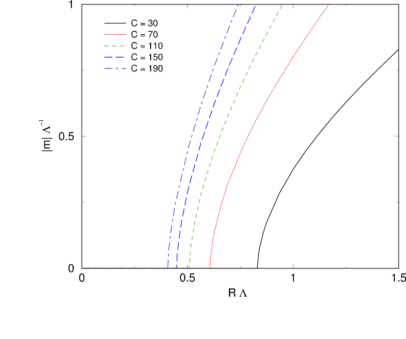
(a)

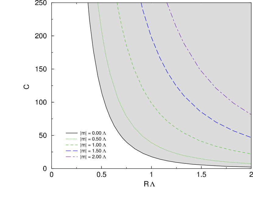
(b)

Figure 6.2: (a) Dynamical fermion mass $m$ as a function of the compactification radius $R$ with the dimensionless coupling $C\equiv\bar{G}/(2\pi R^{3})=G/R^{2}$ fixed. The fermion mass is generated dynamically beyond a critical $R$. (b) Contour curve of $m$. The critical curve is drawn by real line and the massive region is filled.

As was shown in Eq. (6.6) the lowest fermion mass on the four-dimensional brane is $m=Ng\left<|\sigma|\right>$ where $\left<|\sigma|\right>$ is determined by solving Eq. (6.7). The critical curve which represents the critical radius as a function of the coupling constant is shown in Fig. 6.2 as the curve for $m=0$. If we assume $\Lambda\sim 1/R\sim$ TeV like in the large extra dimension scenario [2, 3], light ($\ll$ TeV) fermions are obtained in the region between the solid line and the dot-dashed line in the Fig. 6.2, i.e. just above the critical line of the second phase transition.

6.2.2 Warped bulk

In this section we introduce a bulk fermion $\Psi$ and two fermions $\psi_{1}$ and $\psi_{2}$ on a $y=0$ and a $y=\pi R\equiv L/2$ brane respectively in the RS warped brane world [61, 62]. We consider such two kind of brane fermion $\psi_{1}$ and $\psi_{2}$ because the invariance of replacing two branes each other in the warped dimension is violated, i.e. $\psi_{1}$ has different property from $\psi_{2}$.

Following Chang et al.[61, 62] we derive the mode expansion of the bulk fermion in the RS space-time such that

$$\Psi(x,y)=\frac{e^{3k|y|}}{\sqrt{L}}\sum_{n}\left[\Psi_{L}^{(n)}(x){\xi(y)}+\Psi_{R}^{(n)}(x){\eta(y)}\right],$$ (6.8)

$$\left\{\matrix{{\xi(y)}=\sqrt{\frac{2\pi kR}{1-e^{-\pi kR}}}e^{-k|\pi R-y|}\sin\displaystyle{\frac{m_{n}}{k}}(1-e^{2k|y|})\cr\cr{\eta(y)}=\sqrt{\frac{2\pi kR}{1-e^{-\pi kR}}}e^{-k|\pi R-y|}\cos\displaystyle{\frac{m_{n}}{k}}(1-e^{2k|y|})}\right.,$$

where $m_{n}\equiv{n\pi k}/{(e^{\pi kR}-1)}$. With this expansion the kinetic terms of the KK modes become

$${\cal L\/}^{(4)}_{\rm bluk}=\int dy\,E\bar{\Psi}i\gamma^{M}D_{M}\Psi=\sum_{n}\left[\bar{\Psi}^{(n)}i/\!\!\!\partial\Psi^{(n)}-\frac{m_{n}}{2\pi R}\bar{\Psi}^{(n)}\Psi^{(n)}\right].$$

In the following we adopt the similar analysis to the previous flat case to the RS background.

Now we extend the previous Lagrangian (6.4) to the case in the RS warped background with a vielvein $E_{\bar{M}}^{\ \ M}=\left(\matrix{e^{2k|y|}\eta_{\bar{\mu}}^{\ \mu}&0\cr 0&1}\right)$ whose square becomes the metric $G_{MN}$. Then we start with the following five-dimensional Lagrangian:

$${\cal L\/}^{(5)} = E\bar{\Psi}i\gamma^{M}D_{M}\Psi+E_{(1)}\left[{\bar{\psi}_{1}i\gamma^{\mu}\partial_{\mu}\psi_{1}-\bar{G}_{1}(\bar{\Psi}\gamma^{\mu}\Psi)(\bar{\psi}_{1}\gamma_{\mu}\psi_{1})\,}\right]\delta(y)$$ (6.9)

$$\hskip 28.45274pt+E_{(2)}\left[{\bar{\psi}_{2}i\gamma^{\mu}\partial_{\mu}\psi_{2}-\bar{G}_{2}(\bar{\Psi}\gamma^{\mu}\Psi)(\bar{\psi}_{2}\gamma_{\mu}\psi_{2})\,}\right]\delta(y-\pi R),$$

where $\bar{G}_{1}$ and $\bar{G}_{2}$ is the four-fermion coupling on $y=0$ and $y=\pi R$ brane, respectively. They should satisfy $\bar{G}_{1}=2\pi RG|_{y^{\ast}=0}$ and $\bar{G}_{2}=2\pi RG|_{y^{\ast}=\pi R}$ in our case, i.e. they are induced via the bulk gauge interaction. After chiral rotation $\Psi\to e^{i\frac{\pi}{4}\gamma^{5}}\Psi$ and $\psi_{i}\to e^{i\frac{\pi}{4}\gamma^{5}}\psi_{i}$, we introduce scalar and pseudo-scalar auxiliary fields $\sigma_{i}\sim\bar{\Psi}\psi_{i}$ and $\pi_{i}\sim\bar{\Psi}i\gamma_{5}\psi_{i}$ where $i=1,2$. Here we assume (or from the beginning consider such model) that $\langle\pi_{i}\rangle=0$ because of e.g. the relict from five-dimensional Lorentz invariance. Thus our four-dimensional Lagrangian is rewritten as

$${\cal L\/}^{(5)} = E\bar{\Psi}i\gamma^{M}\partial_{M}\Psi+\left[\bar{\psi_{1}}i/\!\!\!\partial\psi_{1}-N_{f}\left|\sigma_{1}\right|^{2}+(\sqrt{\bar{G}_{1}}\sigma_{1}\bar{\Psi}\psi_{1}+h.c.)\right]\delta(y)$$

$$+e^{-4\pi kR}\left[e^{\pi kR}\bar{\psi_{2}}i/\!\!\!\partial\psi_{2}-N_{f}\left|\sigma_{2}\right|^{2}+(\sqrt{\bar{G}_{2}}\sigma_{2}\bar{\Psi}\psi_{2}+h.c.)\right]\delta(y-\pi R).$$

Now we substitute the mode expansion of $\Psi$ of Eq. (6.8) into the Lagrangian and integrate it over the extra dimension. Taking $e^{-\frac{3}{2}\pi kR}\psi_{2}\to\psi_{2}$ and $e^{-2\pi kR}\sigma_{2}\to\sigma_{2}$, Lagrangian in four-dimension becomes

$${\cal L\/}^{(4)} \equiv \int dy\,{\cal L\/}^{(5)}$$ (6.10)

$$= \sum_{n}\left[\bar{\Psi}^{(n)}i/\!\!\!\partial\Psi^{(n)}-\frac{n}{R}\bar{\Psi}^{(n)}\Psi^{(n)}\right]+\bar{\psi_{1}}i/\!\!\!\partial\psi_{1}+\bar{\psi_{2}}i/\!\!\!\partial\psi_{2}-N_{f}(\left|\sigma_{1}\right|^{2}+\left|\sigma_{2}\right|^{2})$$

$$+\sum_{n}\left(\mu_{1}\bar{\Psi}_{R}^{(n)}\psi_{1}+h.c.\right)+\sum_{n}\left((-1)^{n}\mu_{2}\bar{\Psi}_{R}^{(n)}\psi_{2}+h.c.\right),$$

where

$$\mu_{1}\equiv\displaystyle{\sqrt{\bar{G}_{1}/(2\pi R)}\,\sigma_{1}},\ \ \mu_{2}\equiv\displaystyle{\sqrt{\bar{G}_{2}/(2\pi R)}\,\sigma_{2}},\ \ R_{\rm w}\equiv\frac{1}{m_{1}}=\frac{e^{\pi kR}-1}{\pi k}\sim({\rm TeV})^{-1}.$$

Here we note that even though $\Lambda\sim M_{\rm Pl}$ the mass of the 1st KK excited mode $1/R_{\rm w}$ can be of the order of TeV without fine-tuning because of the warp factor (for $kR\sim 11$) in the RS metric.

After integrating out all fermionic degrees of freedom, we obtain the effective potential for $\sigma_{i}(\mu_{i})$ as follows [59]:

$$\bar{V}({\mu_{1}}/\Lambda,{\rm 5D}/\Lambda)$$

$$= [\,V({\mu_{1}}/\Lambda,{\mu_{2}}/\Lambda)-V(0,0)\,]/\Lambda^{4}$$

$$= 2\pi R\Lambda\left[\frac{({\mu_{1}}/\Lambda)^{2}}{\bar{G}_{1}\Lambda^{3}}+\frac{({\mu_{2}}/\Lambda)^{2}}{\bar{G}_{2}\Lambda^{3}}\right]$$

$$-\frac{1}{2\pi^{2}}\int_{0}^{1}dz\,z^{3}\ln\Bigg{[}1+\frac{\pi R\Lambda}{z}\left\{\left(\frac{{\mu_{1}}}{\Lambda}\right)^{2}+\left(\frac{{\mu_{2}}}{\Lambda}\right)^{2}\right\}\coth(\pi zR\Lambda)$$

$$\hskip 113.81102pt+\frac{\pi^{2}}{2}(R\Lambda)^{2}\left(\frac{{\mu_{1}}}{\Lambda}\right)^{2}\left(\frac{{\mu_{2}}}{\Lambda}\right)^{2}\Bigg{]}.$$

The behavior of the vacuum is determined by solving the gap equations ($i,j=1,2$; $i\neq j$):

$$\frac{\partial\bar{V}}{\partial(\mu_{i}/\Lambda)}$$

$$= R\Lambda\frac{\mu_{i}}{\Lambda}\,\Bigg{\{}\frac{4\pi}{\bar{G}_{i}\Lambda^{3}}-\frac{1}{2\pi}\,\int_{0}^{1}dz\frac{z^{3}(\pi R\Lambda\mu_{j}^{2}\tanh(\pi zR\Lambda)+2)}{z\left\{1+\frac{\pi^{2}}{2}(R\Lambda)^{2}\left(\frac{\mu_{1}}{\Lambda}\right)\left(\frac{\mu_{2}}{\Lambda}\right)\right\}\tanh(\pi zR\Lambda)+\pi R\Lambda\left\{\left(\frac{\mu_{1}}{\Lambda}\right)+\left(\frac{\mu_{2}}{\Lambda}\right)\right\}}\Bigg{\}}$$

$$= 0.$$

The system has a second order phase transition. The phase structure of this system is summarized in the Fig. 6.3. If $\bar{G}_{i}\gtrsim\bar{G}_{i}^{\rm critical}$, we see $\left<\mu_{i}\right>\gtrsim 0$. Therefore we can have three mass scale $\Lambda\sim M_{\rm Pl}$, $R_{\rm w}^{-1}\sim$ TeV and $\left<\mu_{2}\right>\ll$ TeV in the RS brane world if we can realize coupling just above its critical value.

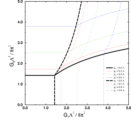
Figure 6.3: The phase structure of the vacuum.

Now we realize that $\mu_{1}$ and $\mu_{2}$ can have nonzero vacuum expectation value and Lagrangian (6.10) has mixing term $\bar{\Psi}_{R}\psi_{i}+{\rm h.c.}$. The physics on the $y=\pi R$ brane is examined by integrating out the invisible field $\psi_{1}$. Setting $\sqrt{2}\Psi^{(n)}_{L}\equiv N^{(n)}-M^{(n)}$ and $\sqrt{2}\Psi^{(n)}_{R}\equiv N^{(n)}+M^{(n)}$ ($n\neq 0$), the effective Lagrangian on the $y=\pi R$ brane is obtained as follows:

$${\cal L\/}^{(4)}_{\rm eff}=\bar{\Theta}_{2}[\,i\partial\!\!\!/+M_{2}+|\mu_{1}|^{2}P\,]\Theta_{2},$$ (6.11)

where $\Theta_{2}^{T}\equiv\left(\psi_{2}\,,\,\Psi^{(0)}_{R}\,,\,N^{(1)}\,,\,M^{(1)}\,,\,N^{(2)}\,,\,M^{(2)}\cdots\right)$ and

$$M_{2}\equiv\left(\matrix{0&\mu_{2}^{*}&-\mu_{2}^{*}&-\mu_{2}^{*}&\mu_{2}^{*}&\mu_{2}^{*}&\cdots\cr\mu_{2}&0&0&0&0&0&\cdots\cr-\mu_{2}&0&\frac{1}{R_{\rm w}}&0&0&0&\cdots\cr-\mu_{2}&0&0&-\frac{1}{R_{\rm w}}&0&0&\cdots\cr\mu_{2}&0&0&0&\frac{2}{R_{\rm w}}&0&\cdots\cr\mu_{2}&0&0&0&0&-\frac{2}{R_{\rm w}}&\cdots\cr\vdots&\vdots&\vdots&\vdots&\vdots&\vdots&\ddots}\right),\quad P\equiv\left(\matrix{0&0&0&\cdots\cr 0&(i\partial\!\!\!/)^{-1}&(i\partial\!\!\!/)^{-1}&\cdots\cr 0&(i\partial\!\!\!/)^{-1}&(i\partial\!\!\!/)^{-1}&\cdots\cr\vdots&\vdots&\vdots&\ddots}\right).$$ (6.12)

We have seen above that the dynamical fermion mass generation is of the second order phase transition, and we find the parameter region of $(\bar{G}_{1},\bar{G}_{2})$ for $0<\left<\mu_{2}\right>\ll\Lambda$, $\left<\mu_{1}\right>=0$. Thus in Eq. (6.11) we have a possibility to get a light (Dirac) fermion by diagonalizing Eq. (6.12) on the $y=\pi R$ brane. We are now treating the case that the four-fermion interactions are induced by a common gauge theory. From Fig. 6.3 we know that we might obtain such result because $\bar{G}_{1}\ll\bar{G}_{2}$ due to the localization effect of the gauge boson KK modes (see Fig. 5.2).

6.3 Discussions: four-fermion approximation

In this chapter we analyzed the effect of heavy KK gauge bosons on the dynamical symmetry breaking using local four-fermion approximation. The chiral phase transition on the brane with [$U(1)$] gauge theory in the bulk is revealed to be of the second order and the critical coupling is less than that of the usual 4D theory. We obtained the basic structure of dynamical symmetry breaking on a brane induced by bulk gauge theory.

We also analyzed the case that there exists a bulk fermion in addition to the brane fermions. In such case it is difficult to analyze the exact gauge NJL approximation and we adopt further approximations. We found that the mixing of the brane fermions with the bulk fermions does not lead to the lightest fermion masses of order $1/R_{\rm w}$ and the dynamically generated fermion masses are not of order $1/R_{\rm w}$ but of order $\left<\mu_{2}\right>$. If we assume that the coupling or compactification radius is near its critical value, $\left<\mu_{2}\right>$ can be much smaller than $\Lambda$ because the dynamical fermion mass generated under the second-order phase transition is small near the critical parameters irrespectively of $\Lambda$ and $1/R_{\rm w}$. In this case the possibility of having low mass fermions resulted from the dynamical origin that is quite different from the ones in other approaches in which low mass fermions are expected to show up as a result of the kinematical origins [70, 71, 72, 73, 74]. In order to apply this dynamical mechanism to realistic problems, however, it seems that we need certain mechanism to realize such a critical value of parameter because the four-fermion coupling $\bar{G}$, compactification radius $R$ and gauge coupling $g$ is related by Eq. (5.22).

In the four-fermion approximation we neglect the kinetic energy of KK gauge bosons that becomes more important as the compactification scale $1/R$ decreases compared with the cut-off scale $\Lambda$. Therefore in the next chapter we will construct another way to treat directly the bulk gauge boson effect on the dynamical symmetry breaking on a brane.

Chapter 7 Analysis of improved ladder Schwinger-Dyson equation

As was shown in the previous chapter, in higher-dimensional gauge theories with compact extra dimensions, the effect of gauge boson KK mode is well approximated by four-fermion interactions between charged matter fermions if the scale of the compactification is less than the cut-off scale of the theory. When we treat the case that the compactification scale is sufficiently small compared with the cut-off scale we can not neglect the effect from the gauge boson kinetic term.

In this chapter we utilize Schwinger-Dyson (SD) [7] equation for analyzing such case. It is equivalent to a self-consistent equation shown in Fig. 7.1 that is derived from an extremum condition of the effective action against the variation by a two-point function (propagator).

Figure 7.1: Schwinger-Dyson equation for a fermion propagator in gauge theory. The filled circles mean that it includes all quantum corrections.

Actually we can not solve the exact SD equation, and in most case we solve it by adopting ladder approximation shown in Fig 7.2 that is obtained by replacing a propagator and vertex function with a tree one except for the target propagator.

Figure 7.2: Ladder Schwinger-Dyson equation for a fermion propagator in gauge theory. The filled circles mean that it includes all quantum corrections.

In the following we apply SD equation to the analyses of a dynamical fermion mass on a boundary in higher-dimensional space-time that is induced by a bulk gauge theory.

7.1 Schwinger-Dyson equation of boundary propagator

From the Lagrangian (5.20) we construct a SD equation for the fermion propagator,

$$iS^{-1}(p)=iS^{-1}_{0}(p)+\sum_{n=0}^{N_{\rm KK}}\int\frac{d^{4}q}{i(2\pi)^{4}}\left[-ig_{n}T^{a}\Gamma^{M}\right]S(q)\left[-ig_{n}T^{a}\Gamma^{N}\right]D_{MN}^{(n)}(p-q),$$ (7.1)

where $T^{a}$ is the gauge group representation matrix of the fermion, and $S_{0}(p)=i/p\!\!\!/$, $S(p)$ and $D_{MN}^{(n)}(p-q)$ are the free fermion propagator, full fermion propagator and full $n$-th excited KK gauge boson propagator respectively. In this thesis we use the ladder approximation in which $D_{MN}^{(n)}$ is replaced by the free propagator,

$$D_{MN}^{(n)}(k) \equiv \frac{-i}{k^{2}-M_{n}^{2}}\left[\eta_{MN}-(1-\xi)\frac{k_{M}k_{N}}{k^{2}-\xi M_{n}^{2}}\right].$$

By writing the full fermion propagator as

$$iS^{-1}(p) \equiv A(-p^{2})p\!\!\!/-B(-p^{2}),$$

the SD equation (7.1) becomes the simultaneous integral equation of $A$ and $B$,

$$A(p^{2}) = 1+\int_{0}^{\Lambda^{2}}dq^{2}\,\frac{q^{2}A(q^{2})}{A^{2}(q^{2})q^{2}+B^{2}(q^{2})}\sum_{n=0}^{N_{\rm KK}}L_{\xi}(p^{2},q^{2};M_{n},\alpha_{n}),$$ (7.2)

$$B(p^{2}) = \int_{0}^{\Lambda^{2}}dq^{2}\,\frac{q^{2}B(q^{2})}{A^{2}(q^{2})q^{2}+B^{2}(q^{2})}\sum_{n=0}^{N_{\rm KK}}K_{\xi}(p^{2},q^{2};M_{n},\alpha_{n}),$$ (7.3)

where [75]

$$L_{\xi}(p^{2},q^{2};M_{n},\alpha_{n}) = \frac{\alpha_{n}}{4\pi}\Bigg{[}q^{2}f_{M_{n}^{2}}^{2}(p^{2},q^{2})+\frac{2q^{2}}{M_{n}^{2}}\left\{f_{M_{n}^{2}}(p^{2},q^{2})-f_{\xi M_{n}^{2}}(p^{2},q^{2})\right\}$$ (7.4)

$$\hskip 28.45274pt-\frac{(q^{2})^{2}+p^{2}q^{2}}{2M_{n}^{2}}\left\{f_{M_{n}^{2}}^{2}(p^{2},q^{2})-f_{\xi M_{n}^{2}}^{2}(p^{2},q^{2})\right\}\Bigg{]},$$

$$K_{\xi}(p^{2},q^{2};M_{n},\alpha_{n}) = \frac{\alpha_{n}}{4\pi}\bigg{[}4f_{M_{n}^{2}}(p^{2},q^{2})+\frac{p^{2}+q^{2}}{M_{n}^{2}}\left\{f_{M_{n}^{2}}(p^{2},q^{2})-f_{\xi M_{n}^{2}}(p^{2},q^{2})\right\}$$ (7.5)

$$\hskip 28.45274pt-\frac{p^{2}q^{2}}{M_{n}^{2}}\left\{f_{M_{n}^{2}}^{2}(p^{2},q^{2})-f_{\xi M_{n}^{2}}^{2}(p^{2},q^{2})\right\}\Bigg{]},$$

$$f_{M}(p^{2},q^{2}) = \frac{2}{p^{2}+q^{2}+M+\sqrt{(p^{2}+q^{2}+M)^{2}-4p^{2}q^{2}}},$$

$$\alpha_{n} \equiv \alpha\chi_{n}^{2}(y^{\ast})\qquad(n\neq 0),$$

$$\alpha_{0} = \alpha=g^{2}/4\pi.$$

Since our analysis is based on the effective theory on the four-dimensional brane below the reduced cutoff, the explicit UV cutoff $\Lambda$ in terms of the loop momentum on the brane appears. $A(x)$ and $B(x)$ are the wave-function normalization factor and the mass function of the fermion respectively. The mass function $B(x)$ is the oder parameter of chiral symmetry breaking on the brane. The chiral symmetry is broken down for $B(x)\neq 0$. By solving Eqs. (7.2) and (7.3) we obtain the behavior of the dynamical fermion mass on the brane.

7.2 Improved ladder analysis of dynamical mass on the boundary

In this section we numerically solve the SD equation and analyze dynamical brane fermion mass induced by the bulk gauge theory [57, 58].

First we analyze the case of the bulk Abelian gauge theory (QED) with $N_{\rm KK}\lesssim 10$ [58], and the results are shown in Sec. 7.2.1. In such case we can use the point vertex approximation depicted in Fig 7.2. Then we proceed to the Yang-Mills case [57]. To solve the SD equation of Yang-Mills theory we use the improved ladder approximation shown in Fig. 7.3 where the running coupling is imposed to the vertex function.

Figure 7.3: Improved ladder Schwinger-Dyson equation for a fermion propagator in gauge theory. The darkly filled circles mean that it includes all quantum corrections. The lightly filled circle means that we put (perturbative) running coupling there.

The running coupling is derived from the truncated KK approach proposed in Ref. [15]. We use the asymptotic form (5.11) of the KK spectrum to evaluate the running coupling in RS brane world.

In Sec. 7.2.2 we review the process of analyzing SD equation in usual 4D QCD [76], and then we extend it to the brane world bulk Yang-Mills theory in Sec. 7.2.3 and 7.2.4. For convenience we choose QCD ($SU(3)_{c}$ Yang-Mills theory with $N_{\rm f}=3$ flavor fermion on the brane) as a concrete example of the bulk Yang-Mills theory, because the bulk results can be compared with the usual 4D QCD. We expect that the essential point of the results is not changed in the other bulk Yang-Mills theory such as technicolor.

To solve Eqs. (7.2) and (7.3) numerically, we employ the iteration method. Starting from suitable trial functions for $A(p^{2})$ and $B(p^{2})$, we numerically evaluate the right-hand sides of Eqs. (7.2) and (7.3). We next use the resulting functions, $A(p^{2})$ and $B(p^{2})$, to calculate the right-hand sides of Eqs. (7.2) and (7.3), and we iterate the calculational procedure until stable solutions were obtained. At each iteration, the integration is performed using the Monte Carlo method, and it is cut off at the mass scale $\Lambda$.

7.2.1 QED in bulk

Figure 7.4: Behavior of the wave-function $A(p^{2}=0.01\Lambda^{2})$ as a function of the coupling constant $\alpha$ for the cases of a flat extra dimension ($R\sim 1/\Lambda$) with $\xi\sim 0.21$ and a warped extra dimension ($2kR\sim 1$) with $\xi\sim 0.23(y=\pi R)$ and $\xi\sim 0.04(y=0)$. (Here $y$ is denoted as a dimensionless coordinate $y/(2\pi R)\to y$.)

Figure 7.5: Behavior of the mass function $B(p^{2}=0.01\Lambda^{2})$ as a function of $\alpha$ for the cases of QED, a flat extra dimension ($R\sim 1/\Lambda$) and a warped extra dimension ($2kR\sim 1$) in the ladder SD equation. (Here $y$ is denoted as a dimensionless coordinate $y/(2\pi R)\to y$.)

Figure 7.6: Behavior of the mass function $B(p^{2}=0.01\Lambda^{2})$ as a function of $\alpha$ for a flat extra dimension with $R=5/\Lambda(N_{\rm KK}=5)$, $R=10/\Lambda(N_{\rm KK}=10)$, $R=15/\Lambda(N_{\rm KK}=15)$ and $R=20/\Lambda(N_{\rm KK}=20)$ in the ladder SD equation.

Figure 7.7: Behavior of the mass function $B(p^{2}=0.01\Lambda^{2})$ as a function of $\alpha$ for a warped extra dimension $(y=\pi R)$ with $1kR=1.80(N_{\rm KK}=5)$, $2kR=2.22(N_{\rm KK}=10)$, $2kR=2.47(N_{\rm KK}=15)$ and $2kR=2.65(N_{\rm KK}=20)$ in the ladder SD equation.

First, we consider the flat extra dimension with $R\sim 1/\Lambda$ and the warped extra dimension with $2kR\sim 1$. In this case only the lightest KK mass is less than the cutoff scale, i.e., $N_{\rm KK}=1$.

If the gauge fields do not propagate in the extra dimension, i.e. if no KK modes exist, the Landau gauge, $\xi=0$, is consistent with the Ward-Takahashi identity for the ladder SD equation. In the bulk gauge theories, massive KK modes appear in the brane, and the Ward-Takahashi identity is not guaranteed within the ladder approximation in the Landau gauge. We attempted to solve the ladder SD equation using various values of the gauge parameter $\xi$. As illustrated in Fig. 7.5, it is possible to choose the gauge parameter $\xi=\xi_{WT}$ for which the fermion wave-function $A(p^{2})$ is almost unity, and the Ward-Takahashi identity nearly holds on the brane [58]. In the models considered here, $\xi_{WT}$ is given by $\xi_{WT}\sim 0.21$ (flat,$R\sim 1/\Lambda$), $\xi_{WT}\sim 0.31$ (warped,$2kR\sim 1;\ y=\pi R$), and $\xi_{WT}\sim 0.11$ (warped,$2kR\sim 1;\ y=0$). In the following we consider the gauge parameter $\xi=\xi_{WT}$.

To study the structure of the chiral phase transition, we observe the behavior of the mass function $B(p^{2})$ at some fixed value of $p$. The $\alpha$ dependence of the mass function $B(p^{2})$ with $p^{2}=0.01\Lambda^{2}$ is plotted in Fig. 7.5. As seen there, the chiral phase transition is of the second order (or continuous), since a fermion mass is generated at a critical value of the coupling constant $\alpha$ without any discontinuity. In the $y=0$ brane in the warped extra dimension, the lightest KK mode increases the mass function $B(p^{2})$, but the result yields no large difference from that for QED. On the $y=\pi R$ brane in the warped extra dimension and on the brane in the flat extra dimension, the results differ significantly from QED. In these two cases, the critical coupling $\alpha_{\rm critical}$ is less than that in QED. This is due to the large effective coupling $\alpha_{1}\sim 2.0\alpha$ for the lightest KK mode. Comparing Fig. 6.1 with Fig. 7.5, we observe that the result for the ladder SD equation is qualitatively consistent with that obtained with the local four-fermion approximation in the previous section but the latter case overestimates the effect of the KK excited modes on the chiral phase transition. We see that the propagation of the KK mode weakens the effect on the phase transition [58].

Next, we study how the number of KK modes, $N_{\rm KK}$, affects the chiral phase transition. (We recall that $N_{\rm KK}$ is the number of KK modes with mass less than the cutoff scale $\Lambda$.) Here we consider the SD equation in the flat extra dimension with $R\sim 5/\Lambda,10/\Lambda,15/\Lambda,20/\Lambda$. Obviously, $N_{\rm KK}$ for these radii is given by $5,10,15$ and $20$, respectively. In the warped extra dimension, the KK mode mass depends on the RS compactification scale, $L=2\pi R$. We also evaluate the SD equation in the warped extra dimension, where $N_{\rm KK}$ is equal to $5,10,15$ and $20$ for the corresponding radii. By solving KK eigenvalue equation it is found that these values of $N_{\rm KK}$ are realized for $2kR\sim 1.80,2.22,2.47$ and $2.65$, respectively. Here we assume that the heaviest KK mode mass is near the cutoff scale.

In models with $N_{\rm KK}=5,10,15$ and $20$, the gauge parameter for which the fermion wave-function is almost unity is given by $\xi_{WT}\sim$ $0.285$ (flat), $0.288$ (warped, $y=\pi R$) for $N_{\rm KK}=5$, $\xi_{WT}\sim$ $0.275$ for $N_{\rm KK}=10$, $\xi_{WT}\sim$ $0.274$ for $N_{\rm KK}=15$ and $\xi_{WT}\sim$ $0.272$ for $N_{\rm KK}=20$. using the gauge parameter $\xi=\xi_{WT}$, we solved Eqs. (7.2) and (7.3) numerically. In Figs. 7.7 and 7.7 we illustrate the behavior of the mass function $B(p^{2})$ for the flat extra dimension and for the $y=\pi R$ brane in the warped extra dimension. Assuming the critical exponent is 0.5, the critical coupling $\alpha_{\rm critical}$ with $N_{\rm KK}=5$, $10$, $15$ and $20$ is evaluated, respectively, as [58]

$$\alpha_{\rm critical} = 0.275,\ 0.140,\ 0.094\textrm{ and }0.071\textrm{ (flat)},$$

$$\alpha_{\rm critical} = 0.187,\ 0.078,\ 0.048\textrm{ and }0.034\textrm{ (warped; $y=\pi R$ )}.$$

In both brane models, chiral symmetry breaking is enhanced by KK mode summation, and the critical coupling approaches the ordinary electromagnetic coupling constant $\sim 1/137$ as $N_{\rm KK}$ increases.

7.2.2 QCD in 4D

Next we review the analysis of QCD in four-dimension. The main difference between the case of QCD and QED is the existence of the gauge boson self couplings. We incorporate it by introducing running coupling on the vertex in the improved SD equation. Taking $N_{\rm KK}=0$ in Eqs. (7.2) and (7.3), the SD equation for usual QCD in four dimensional space-time (i.e. QCD on the brane) is obtained. In this case the integration kernels (7.4) and (7.5) become

$$L_{\xi}(p^{2},q^{2};M_{0}=0,\alpha_{0}=\alpha) = \frac{\alpha}{4\pi}\,\xi\,q^{2}\,f_{0}^{2}(p^{2},q^{2}),$$ (7.6)

$$K_{\xi}(p^{2},q^{2};M_{0}=0,\alpha_{0}=\alpha) = \frac{\alpha}{4\pi}\,(3+\xi)\,f_{0}(p^{2},q^{2}),$$ (7.7)

where

$$f_{0}(p^{2},q^{2}) = \theta(p^{2}-q^{2})\frac{1}{p^{2}}+\theta(q^{2}-p^{2})\frac{1}{q^{2}}.$$

We usually use Landau gauge $\xi=0$ that results in $L_{\xi}(p^{2},q^{2};M_{0}=0,\alpha_{0}=\alpha)=0$, i.e. $A(p^{2})=1$ in the SD equation. In that case the SD equation becomes single equation only with $B(p^{2})$. $A(p^{2})=1$ satisfies the QED like Ward-Takahashi identity.

We put the running coupling on the vertex function in the SD equation to compensate for neglecting three and four point gluon self interactions ${\cal L}_{\rm SI}$ in the ladder approximation. That is so called improved ladder approximation. We use the one-loop perturbative running coupling,

$$\alpha\equiv\frac{\pi}{3C_{2}(F)}\lambda(k^{2}),$$

where

$$\lambda(z) = \frac{\lambda_{0}}{1+\lambda_{0}B\ln\frac{z}{\mu^{2}}},$$

and $B=\frac{4\pi^{2}}{3C_{2}(F)}\beta_{0}$. We define $\beta_{0}$ by $\beta(g)=-\beta_{0}g^{3}+{\cal O}(g^{5})$ and $\beta_{0}=\frac{1}{16\pi^{2}}\big{[}\frac{11}{3}C_{2}(G)-\frac{4}{3}N_{\rm f}T(F)\big{]}$ where $G$ and $F$ stand for the gauge group and the fermion representation under the group respectively. $C_{2}(G)$, $C_{2}(F)$ and $T(F)$ are defined by $\sum_{c,d}f_{acd}f_{bcd}\equiv C_{2}(G)\delta_{ab}$, $\textrm{tr}(T^{a}T^{b})\equiv T(F)\delta_{ab}$ and $\sum_{a}T^{a}T^{a}\equiv C_{2}(F)1$. In the case that $G=SU(N=3)$ and $F$ is fundamental representation, these values are given by

$$C_{2}(G)=N=3,\quad T(F)=\frac{1}{2},\quad C_{2}(F)=\frac{N^{2}-1}{2N}=4/3,$$

$$B=\frac{1}{12C_{2}(F)}\left(\frac{11N-2N_{\rm f}}{3}\right)=\frac{9}{16},\quad(N=3,N_{\rm f}=3).$$

We also define $\Lambda_{\rm QCD}$, the dynamical scale of QCD, as

$$\frac{1}{\lambda(z)}-B\ln z=\frac{1}{\lambda_{0}}-B\ln\mu^{2}\ \equiv\ -B\ln\Lambda_{\rm QCD}^{2},\qquad\left(\Lambda_{\rm QCD}^{2}\equiv\mu^{2}/e^{\frac{1}{\lambda_{0}B}}\right),$$

and obtain

$$\lambda(z) = \frac{16}{9}\frac{1}{\ln(z/\Lambda_{\rm QCD}^{2})}.$$ (7.8)

Following the analysis in Ref. [77] we introduce IR cutoff $z_{\rm IF}$ in the running coupling as

$$\alpha(z) = \frac{\pi}{3C_{2}(F)}\left[\theta(z_{\rm IF}-z)\lambda(z_{\rm IF})+\theta(z-z_{\rm IF})\lambda(z)\right],$$

and we take the following approximation

$$\alpha \to \alpha(z)\simeq\alpha(x+y),$$ (7.9)

in the integration kernel (7.6) and (7.7). It is called Higashijima-Miransky approximation. This is due to the consideration that the mean value of the $\theta$-dependent part in $\alpha(z)$ where $z=x+y-\sqrt{xy}\cos\theta$ has only a negligible effect after the angle integration in the SD equation. It is known that the approximation (7.9) violates the chiral Ward-Takahashi identity. In this thesis we choose the gauge parameter $\xi$ to nearly hold the chiral Ward-Takahashi identity. In the following numerical analyses we use the experimental value

$$\Lambda_{\rm QCD}\simeq 200\textrm{ MeV},$$

and choose $\ln(z_{\rm IF}/\Lambda_{\rm QCD}^{2})=1$ for the IR cutoff.

The composite Nambu-Goldstone field corresponds to the composite Higgs field in the dynamical electroweak symmetry breaking scenario. Its decay constant is obtained by the Pagels-Stokar approximation [78],

$$f_{\pi}^{2}=\frac{N}{4\pi^{2}}\int_{0}^{\Lambda^{2}}xdx\frac{B(x)\left(B(x)-xB^{\prime}(x)/2\right)}{\left(A^{2}(x)x+B^{2}(x)\right)^{2}}.$$ (7.10)

Here we show the numerical results of the improved ladder SD equation in 4D QCD. We set the cutoff scale $\Lambda=10$ TeV in order to compare with the result of the brane world models. By using the replacement (7.9) we solve the SD equation (7.2), (7.3) and calculate the mass function $B(x)$. The behavior of the mass function $B(x)$ is shown as the thin solid line in Fig. 7.9. The scale of the fermion mass function is a little bit smaller than the QCD scale, $B(x=\Lambda_{\rm QCD}^{2})\sim{\cal O}(\Lambda_{\rm QCD}/10)$. Substituting the obtained mass function $B(x)$ to Eq. (7.10) we obtain the decay constant of the composite scalar field. As is shown with the thin solid line in Fig. 7.10, the decay constant of 4D QCD is also smaller than the QCD scale, $f_{\pi}\sim{\cal O}(\Lambda_{\rm QCD}/100)$. Since it is the result of the ordinary 4D QCD, the decay constant is too small as Higgs field to break electroweak symmetry.

Figure 7.8: The behavior of $B(x)$ with various bulk space-time derived from the improved ladder SD equation. The case of (4D usual) QCD, bulk QCD in the flat brane world with $(4+\delta)$-dimensional bulk space-time ($\delta=1,2,3,4$) and in the RS brane world are shown. We set $\Lambda_{\rm QCD}=200$ MeV for all cases. The cutoff is taken as $\Lambda=\Lambda_{\rm(4+\delta)D}=10$ TeV for QCD $(\delta=0)$ and flat case $(\delta\neq 0)$, and for the flat brane world we take universal radii $R\Lambda_{\rm(4+\delta)D}=1$. For the RS brane world we take $k=\Lambda_{\rm 5D}=M_{\rm Pl}=10^{16}$ TeV and $\Lambda=\pi e^{-\pi kR}\Lambda_{\rm 5D}=10$ TeV $(kR=11.35)$.

Figure 7.9: The behavior of $A(x)$ with various bulk space-time derived from the improved ladder SD equation. The case of (4D usual) QCD, bulk QCD in the flat brane world with $4+\delta$ dimensional bulk space-time ($\delta=1,2,3,4$) and in the RS brane world are shown. The mass parameters are taken as the same in the caption in Fig. 7.9. In order to satisfy Ward-Takahashi identity, i.e. $A(x)\simeq 1$ within $\pm 5$%, we take the gauge fixing parameter $\xi=0$ for QCD, $\xi=0.02$, $0.07$, $0.57$ and $0.63$ for flat brane world with $\delta=1$, $2$, $3$ and $4$ respectively and $\xi=0.50$ for RS case.

Figure 7.10: The behavior of the decay constant $f_{\pi}$ of the composite scalar field with various bulk space-time derived from the Pagels-Stokar formula. The case of (4D usual) QCD, bulk QCD in the flat brane world with $(4+\delta)$-dimensional bulk space-time ($\delta=1,2,3,4$) and in the RS brane world is shown together. The parameters are taken as the same in the caption in Fig. 7.9.

7.2.3 QCD in flat bulk

Now we analyze the dynamical fermion mass induced by the bulk Yang-Mills theory in flat brane world, $M_{4}\times T^{\delta}$ [57]. For simplicity we set the same radii for all extra directions, i, e, universal extra dimensions. We study $SU(N=3)$ bulk Yang-Mills theory (QCD) with $N_{f}=3$ flavor fermion as a concrete example. For QCD extended in the compact extra dimension with the radius $R$, the running coupling $\alpha(z)$ has the power low behavior [15] in the region $1/R^{2}\leq z$,

$$\alpha^{-1}(z) = \alpha^{-1}_{0}+2\pi\beta_{0}\ln\frac{z}{\mu_{0}^{2}}-2\pi\tilde{\beta}_{0}\ln\frac{z}{\mu_{R}^{2}}+2\pi\tilde{\beta}_{0}\frac{2X_{\delta}}{\delta}\left[\left(\frac{z}{\mu_{R}^{2}}\right)^{\delta/2}-1\right],$$

where $\mu_{R}=1/R$ and

$$X_{\delta} = \frac{\pi^{\delta/2}}{\Gamma(1+\delta/2)}=\frac{2\pi^{\delta/2}}{\delta\Gamma(\delta/2)},\quad\alpha_{0}\equiv\alpha(\mu_{0}^{2}),$$

and $\tilde{\beta}_{0}$ is the beta-function coefficient stimulating from the bulk fields. Thus we obtain the running coupling of the bulk QCD with $N_{\rm f}=3$ flavor fermion on the brane,

$$\lambda(z) = \frac{1}{B\ln(z/\Lambda_{\rm QCD}^{2})-\widetilde{B}\left[\ln(z/\mu_{R}^{2})-\frac{2X_{\delta}}{\delta}\left\{(z/\mu_{R}^{2})^{\delta/2}-1\right\}\right]\theta(z-\mu_{R}^{2})},$$ (7.11)

where

$$\left\{\begin{array}[]{l}B=\frac{1}{24C_{2}(F)}\left(\frac{11N-2N_{\rm f}}{3}\right)=9/16\quad(N=3,N_{\rm f}=3)\\ \widetilde{B}=\frac{1}{24C_{2}(F)}\left(\frac{11N-2\tilde{N}_{\rm f}}{3}\right)=11/16\quad(N=3,\tilde{N}_{\rm f}=0)\end{array}\right..$$ (7.13)

Using the running coupling (7.11), we numerically solve the improved ladder SD equation and find the behaviors of the fermion wave-function $A(x)$ and the mass function $B(x)$ on the brane. We analyze the SD equation on the $(y_{1}^{\ast},\ldots,y_{\delta}^{\ast})$ $=(0,\ldots,0)$ brane, with $\Lambda=\Lambda_{\rm(4+\delta)D}=10$ TeV, $\Lambda_{\rm QCD}=200$ MeV and $R\Lambda_{\rm(4+\delta)D}=1$ as typical cases, where $\Lambda_{\rm(4+\delta)D}$ and $\Lambda$ are the bulk fundamental scale and the reduced cutoff scale on the brane respectively. For $\delta=1,2,3$ and $4$, the behavior of $B(x)$ and $A(x)$ are drawn in Figs. 7.9 and 7.9 respectively. For $\delta<3$ the fermion mass function behaves like 4D QCD, i.e. $B(x=\Lambda_{\rm QCD}^{2})\sim{\cal O}(\Lambda_{\rm QCD}/10)$. For $\delta\geq 3$ the situation is dramatically changed. The fermion mass function develops a value near the reduced cutoff scale, $B(x=\Lambda_{\rm QCD}^{2})\sim{\cal O}(\Lambda)$. Using the Pagels-Stokar formula (7.10), we calculate the decay constant of the composite scalar field. As is shown in Fig. 7.10 the scale of the decay constant is summarized as $f_{\pi}\sim{\cal O}(\Lambda_{\rm QCD}/10)$ for $\delta<3$ and $f_{\pi}\sim{\cal O}(\Lambda/10)$ for $\delta\geq 3$. Therefore if the bulk space-time has seven or more dimensions, the bulk Yang-Mills theory induces the TeV scale decay constant on the brane [57]. There is a possibility that the bulk QCD or technicolor can provide a composite Higgs field in the flat brane world. In this section we take $1/R=\Lambda=\Lambda_{\rm(4+\delta)D}=10$ TeV. We comment that this setup merges into the scenario of ‘large extra dimension’ [2, 3] in which the fundamental scale is around TeV and we assume the existence of a large extra dimension where only the gravity propagates.

7.2.4 QCD in warped bulk

Here we study the bulk QCD in the RS brane world [57]. In the warped brane world a mass scale $\Lambda$ on the brane at $y=y^{\ast}$ is suppressed by the warp factor, i.e. $\Lambda\simeq W(y^{\ast})\Lambda_{\rm 5D}$, where $\Lambda_{\rm 5D}$ is the fundamental scale of the theory and $W(y)=e^{-\pi k|y|}$ is the warp factor. As is discussed in the previous subsection, it is natural to consider that the effective theory of the brane fermion should be regularized by the reduced fundamental scale on the brane. Hence we cutoff the loop momentum in the SD equation at the reduced cutoff scale $\Lambda$ on the brane,

$$\Lambda\simeq e^{-k|y^{\ast}|}\Lambda_{\rm 5D}\simeq e^{-k|y^{\ast}|}k\qquad(y^{\ast}=0,\pi R).$$

For $kR\simeq 11$, UV cutoff scale $\Lambda$ is suppressed by $10^{-15}$ on the $y^{\ast}=\pi R$ brane. Randall and Sundrum obtain the weak and Planck hierarchy form this warp suppression factor in the original RS model [10].

The behavior of the running coupling is nontrivial in the RS space-time. In this thesis we evaluate it in terms of the 4D effective theory below the cutoff scale $\Lambda$ by using the truncated KK approach. In the region $kR\gg 1$ and $M_{n}\ll k$, KK mass spectrum of the gauge boson reduces to the asymptotic form (5.11). Comparing it with the torus case (5.9), we find that the running coupling in the RS space-time is obtained by replacing $\mu_{R}$ with $\mu_{kR}$ and shifting the KK lowest threshold by $\mu_{kR}/4$. In addition we must take the orbifold condition into account. It drops all the $Z_{2}$ odd modes. Only a half contribution comes from the KK excited modes. Thus we replace $\widetilde{B}\to\widetilde{B}/2$ in Eq. (7.11). The running coupling reads

$$\lambda(z)=\frac{1}{B\ln(z/\Lambda_{\rm QCD}^{2})-(\widetilde{B}/2)\left[\ln(\sqrt{z}/\mu_{kR}+1/4)^{2}-4\left\{\sqrt{z}/\mu_{kR}-3/4\right\}\right]\theta(z-(3/4)^{2}\mu_{kR}^{2})},$$ (7.14)

where $B$ and $\widetilde{B}$ are given by Eq. (7.13).

Applying the truncated running coupling (7.14) we evaluate the SD equation on the $y=\pi R$ brane, with $k=\Lambda_{\rm 5D}=M_{\rm Pl}=10^{16}$ TeV, $\Lambda=\pi e^{-\pi kR}\Lambda_{\rm 5D}=10$ TeV and $\Lambda_{\rm QCD}=200$ MeV as typical cases. The solution of $B(x)$ and $A(x)$ are plotted in Figs. 7.9 and 7.9 respectively [57]. Calculating the Eq. (7.10) we obtain the decay constant of the composite scalar as is shown in Fig. 7.10. In the RS brane world both scales of the fermion mass function and the decay constant are near the reduced cutoff scale, $B(x=\Lambda_{\rm QCD}^{2})\sim{\cal O}(\Lambda/10)$, $f_{\pi}\sim{\cal O}(\Lambda/10)$ $\sim$ ${\cal O}(1)$ TeV. Therefore the bulk Yang-Mills theory induces TeV scale decay constant on the brane [57]. It means that the bulk QCD has possibility to realize the composite Higgs scenario of electroweak symmetry breaking.

The original theory has only the Planck scale, it has no TeV scale source but the fermion mass and decay constant of the composite scalar are generated at TeV scale through the warp suppression of the reduced cutoff scale on the $y=\pi R$ brane. KK excited modes of the gauge field are localized at the $y=\pi R$ brane in RS model. It enhances the contribution from the KK modes and realize the TeV scale composite scalar on the brane with only one extra dimension. This is the difference from the (4+1)-dimensional flat brane world, $\delta=1$. The bulk gauge theory with only Planck scale in RS brane world can acquire a TeV scale dynamically due to a fermion pair condensation on the $y=\pi R$ brane through the effect of the gauge boson KK excited modes localized at the brane. The warp suppression mechanism in the RS model is realized dynamically.

The extension of above results to the bulk SM gauge fields will make us to propose two types of primary models of dynamical electroweak symmetry breaking. We call one of them (1,2)-3 model in which the first and second generations in the SM are confined on the $y=0$ brane, and the third generation is on the $y=\pi R$ brane (see Fig. 7.14). The KK excited mode is not localized on the $y=0$ brane shown in Fig. 5.2. The coupling between the KK excited gluons and the brane fermion are suppressed by the mode function $\chi_{n}(y=0)$ on the $y=0$ brane. Therefore we expect that the top quark-pair is condensed on the $y=\pi R$ brane, while the up and charm quark are not condensed. The top mode SM [17] can be realized in RS brane world [56]. We note that the zero modes function, $\chi_{0}$, are constant, so that the fermions on the both brane equally couples to the massless gauge filed (see also Fig. 5.2). We can construct the other model, (1,2,3)-4 model, which is defined as follows. All the SM fermions lie in $y=0$ brane and the fourth generation (or the technifermion) lies in the $y=\pi R$ brane. In this model the fourth generation can develops TeV scale mass function and decay constant by KK excited gluons (or techni-gluons).

It is expected that these models can provide composite Higgs and the TeV scale physics simultaneously. Although some problems are remained, e.g. how to dynamically realize the detailed mass relation (dynamical Yukawa couplings) in SM, or flavor breaking etc..

Figure 7.11: The behavior of $B(x)$ with $(4+1)$-dimensional bulk space-time derived from the improved ladder SD equation. The case of $(4+1)$-dimensional bulk QCD in the flat brane world with the radius $R\Lambda_{\rm 5D}$$=1,2,5$ and $10$, and the case in the RS brane world with the AdS₅ curvature radius $k^{-1}\Lambda_{\rm 5D}$$=1,2,5$ and $10$ are shown. We set $\Lambda_{\rm QCD}=200$ MeV for all cases. The cutoff is taken as $\Lambda=\Lambda_{\rm 5D}=10$ TeV for flat case. For the RS brane world we take $k=\Lambda_{\rm 5D}=M_{\rm Pl}=10^{16}$ TeV and $\Lambda=\pi e^{-\pi kR}\Lambda_{\rm 5D}=10$ TeV $(kR=11.35)$.

Figure 7.12: The behavior of $A(x)$ with $(4+1)$-dimensional bulk space-time derived from the improved ladder SD equation. The case of $(4+1)$-dimensional bulk QCD in the flat brane world with the radius $R\Lambda_{\rm 5D}$$=1,2,5$ and $10$, and the case in the RS brane world with the AdS₅ curvature radius $k^{-1}\Lambda_{\rm 5D}$$=1,2,5$ and $10$ are shown. The mass parameters are taken as the same in the caption in Fig. 7.12. In order to satisfy Ward-Takahashi identity, i.e. $A(x)\simeq 1$ within $\pm 7$%, we take the gauge fixing parameter $\xi=0.020$, $0.040$, $0.080$ and $0.104$ for flat brane world with $R\Lambda_{\rm 5D}=1$, $2$, $5$ and $10$ respectively, and $\xi=0.35$, $0.37$, $0.41$ and $0.50$ for RS brane world with $k^{-1}\Lambda_{\rm 5D}=1$, $2$, $5$ and $10$ respectively.

Figure 7.13: The behavior of the decay constant $f_{\pi}$ of the composite scalar field with $(4+1)$-dimensional bulk space-time derived from the Pagels-Stokar formula. The case of $(4+1)$-dimensional bulk QCD in the flat brane world with the radius $R\Lambda_{\rm 5D}$$=1,2,5$ and $10$, and the case in the RS brane world with the AdS₅ curvature radius $k^{-1}\Lambda_{\rm 5D}$$=1,2,5$ and $10$ are shown together. The parameters are taken as the same in the caption in Fig. 7.12.

7.2.5 Behavior and classification of dynamical mass

The behaviors of $B(x)$ shown in Fig. 7.9 are divided into two pieces. QCD in the flat bulk space-time with $\delta=1$ and $2$ is classified into Yang-Mills type, i.e. the contribution from the KK modes is extremely small and $B(x)$ has a similar profile to the ordinary QCD (QCD on the brane). On the other hand, flat bulk space-time with $\delta=3$, $4$ and the RS brane world are NJL type, i.e. KK modes contribution dominates the symmetry breaking [57].

In Figs. 7.9, 7.9 and 7.10, we consider only the case $N_{\rm KK}=1$. Finally we analyze the $R$- and $k$-dependence of the wave-function $A(x)$ and the mass function $B(x)$ on the brane embedded in (4+1)-dimensional bulk space-time. The behaviors of $A(x)$ and $B(x)$ are shown in Figs. 7.12, 7.12 and 7.13. There are little $R$- and $k$-dependence. Only a small $N_{\rm KK}$-dependence is observed in the behavior of $B(x)$. Eqs. (5.9) or (5.11) show that the number of the KK mode $N_{\rm KK}$ increases as $R$ or $k^{-1}$ increases. The influence of the KK mode propagation seems to be enhanced for larger $R$ or $k^{-1}$. In Fig. 7.12 we clearly observe that the mass function $B(x)$ grows up as $R$ or $k^{-1}$ increases. In Eqs. (7.11) or (7.14) the power low running terms contain the step function $\theta(z-\mu_{R}^{2})$ or $\theta(z-(3/4)^{2}\mu_{kR}^{2})$. Since the KK mode mass scale $\mu_{R}$ and $\mu_{kR}$ are proportional to $1/R$ and $k$ respectively, the contribution from these terms is enhanced as $R$ or $k^{-1}$ increases. The contribution from the power low running suppresses dynamical symmetry breaking. For example, if we drop the power low running term in $(4+1)$-dimensional flat bulk space-time, $B(x)$ blows up from the Yang-Mills type to the NJL type as $N_{\rm KK}$ increases. Thus we conclude that the bulk gluon self interactions ${\cal L}_{\rm SI}$, i.e. the power low running coupling, act as a suppression factor for the dynamical mass on the brane [57].

7.3 Discussions: pion and Higgs boson from single theory

We have studied the basic structure of dynamical symmetry breaking on the four dimensional brane in the bulk Yang-Mills theory (QCD). Using the 4D effective theory of the bulk QCD and the improved ladder SD equation, we have found that the dynamical mass scale can be affected by the reduced cutoff scales on the brane. Starting from the Yang-Mills theory in $M_{4}\times T^{\delta}$ space-time which couples to a fermion on the four dimensional brane we derive four dimensional effective theory by KK reduction. We take $A_{3+i}=0$ $(i=1,\ldots,\delta)$ gauge in extra directions but leave the gauge fixing parameter free parallel to the brane. Our system needs a proper regularization because it is a theory beyond four dimensional space-time where the gauge theory is nonrenormalizable. We impose the cutoff regularization at the UV reduced scale $\Lambda$ on the brane fermion lives in. For the flat brane world the reduced scale should be equal to the fundamental scale in the original bulk Yang-Mills theory, i.e. $\Lambda\simeq\Lambda_{\rm(4+\delta)D}$. The RS brane world, however, has a reduced scale suppressed by the warp factor, that is $\Lambda\simeq e^{-k|y^{\ast}|}\Lambda_{\rm 5D}$ which depends on the position in the extra direction.

Based on the 4D effective theory we derive the SD equation for the fermion propagator on the brane. From the four dimensional point of view the equation corresponds to the simultaneous integral equation. The loop integral consists of one massless and $N_{\rm KK}$ massive vector field where $N_{\rm KK}$ is the number of the KK modes under the reduced cutoff scale. Using the iteration method we numerically solve it for typical values of radius, $R\Lambda_{\rm(4+\delta)D}=1$, and the (AdS) curvature scale, $k=\Lambda_{\rm 5D}$. In order to make the analysis consistent with the QED like Ward-Takahashi identity, we choose the appropriate value of the gauge fixing parameter for each analysis.

The results of the numerical analysis is as follows. For a flat extra dimension $\delta=1$ the dynamical mass of the brane fermion is the same scale as the usual 4D QCD result, i.e. there is little contribution from the KK excited gauge boson. We also study the case of the flat brane world with more than one extra dimension. The numerical analysis of the SD equation shows that the number of the extra dimension must be no less than three, $\delta\geq 3$, to generate the TeV scale dynamical fermion mass on the brane. Therefore it is obtained in the case of the Yang-Mills theory in seven or more dimensional bulk space-time.

Figure 7.14: Dynamical realization of both pion and electroweak Higgs boson from single theory; QCD in warped brane world. Although the RS warped brane world has only one fundamental scale $M_{\rm Pl}$, we might have both the scale of pion and electroweak Higgs boson via bulk QCD dynamics if we assume that the 3rd generation lives on $y=\pi R$ brane while the 1st and 2nd generation live on $y=0$ brane. This is because the gauge boson KK modes are localized at $y=\pi R$ brane while the gauge boson zero mode is flat in extra direction (see Fig 5.2). Then the 1st and 2nd generation decouple from the KK gauge bosons. The electroweak scale is realized by the RS warp factor while the pion scale is given by the usual (4D) QCD dynamics via dimensional transmutation from the logarithmically running coupling.

The RS brane world has one extra dimension which corresponds to $\delta=1$ case but it is curved. Because the gauge boson KK excited modes localized at the $y=\pi R$ brane due to the curvature effect (see Fig.5.2), we have a significant result. The dynamical mass of the brane fermion at the $y=\pi R$ is the order of the reduced cutoff scale that is warp suppressed from the fundamental scale [57]. We also estimate the decay constant of the composite Nambu-Goldstone scalar field by using the Pagels-Stokar approximation [78]. The decay constant is also warp suppressed on the $y=\pi R$ brane in the RS brane world. If the chiral symmetry is gauged as in the SM case, the composite scalar absorbed in the longitudinal component of the gauge boson. This decay constant is directly related to the mass of the gauge boson. The result in the RS brane world provides a possibility to realize the situation that electroweak symmetry breaking is triggered by the condensation of the composite Higgs field on the $y=\pi R$ brane. Such a mechanism is caused by the bulk Yang-Mills theory, for example the technicolor or the QCD itself in the SM (for the latter case, see Fig. 7.14). Therefore we can solve the weak and Planck hierarchy from the warp factor, that is realized, in a sense, dynamically. This is one of the dynamical realization of so called Randall-Sundrum model.

Our analyses are based on the 4D effective theory of the bulk gauge theory with an explicit UV cutoff in the loop momentum integration. We can also check the regularization dependence of our model by comparing the results of the lattice regularized (deconstructed) version. The deconstructed bulk field theory on the RS background [80] will be given in Part III of this thesis.

The results of our analysis are also important in a theoretical sense. We consider that the SD equation includes certain nonperturbative effect of the theory. The nontrivial results obtained here implies that the bulk gauge theory may have rich nonperturbative dynamics that depends on the configurations of the extra space. In the brane world we should take account of such effect in addition to the perturbative analysis. Our results imply that the bulk gauge dynamics can induce various types of the dynamical symmetry breaking in the brane world, depending on the bulk-brane configuration. For instance, we may obtain the dynamical breaking of the grand unification gauge symmetry [81] (or even supersymmetry?), in addition to the possibility of dynamical electroweak symmetry breaking emphasized in this thesis. We are also interested in the consistency of these models with the realistic D-brane system in the string theory.

Part III Higher-dimensional nature in four-dimension

Chapter 8 Warped gauge theory

In part I and II of this thesis we have studied SUSY and nonSUSY gauge theory in higher-dimensional space-time with some boundary terms. We have seen that extra dimensional configurations e.g. wave function localization due to boundary terms or curvature of extra dimension play important role in spontaneous or dynamical symmetry breaking in bulk and boundary system. However the gauge theory in more than four-dimensional space-time is nonrenormalizable and has less predictability. We should consider that the underlying theory such as string theory gives appropriate regularization to such higher-dimensional effective theory.

In Part III of this thesis we give one of such regularization by latticizing the extra dimensions, that is so called deconstruction. For a finite lattice spacing the gauge theory is defined in four-dimensional space-time and is renormalizable. It may also be interesting that we treat such four-dimensional theory as an underlying theory just above the cut off scale of the effective ‘higher-dimensional’ theory considered previously.

We formulate the four-dimensional gauge theory which induces, effectively, a gauge theory in (five-dimensional) general warped background [80]. We call such four-dimensional gauge theory ‘warped gauge theory’. It is interesting that the warped gauge theory gives a wave function localization in the index space of the product gauge group.

8.1 4D formulation for curved geometries

Following Refs. [82, 83], we introduce $SU(n)_{i}$ gauge theories with gauge couplings $g_{i}$ ($i=1,\cdots,N$), and scalar fields $Q_{i}$ ($i=1,\cdots,(N-1)$) which are in bi-fundamental representations of $SU(n)_{i}\times SU(n)_{i+1}$. The system is schematized by the segment diagram in Fig. 8.1.

Figure 8.1: Moose diagram for bulk vector fields in the orbifold extra dimension.

The gauge invariant kinetic term of the scalars $Q_{i}$ is written by

$${\cal L} = \sum_{i=1}^{N-1}(D_{\mu}Q_{i})^{\dagger}(D^{\mu}Q_{i}),$$ (8.1)

where the covariant derivative is given by $D_{\mu}Q_{i}=\partial_{\mu}Q_{i}-ig_{i}A^{i}_{\mu}Q_{i}+ig_{i+1}Q_{i}A^{i+1}_{\mu}$. We assume that the scalar fields $Q_{i}$ develop their VEVs proportional to the unit matrix, $\langle Q_{i}\rangle=v_{i}$, which break the gauge symmetry to a diagonal $SU(n)_{diag}$. From the kinetic term (8.1), the mass terms for the vector fields $A_{\mu}^{i}$ are obtained

$${\cal L}_{gm} = \frac{1}{2}\sum_{i=1}^{N-1}\Big{|}v_{i}(g_{i+1}A_{\mu}^{i+1}-g_{i}A_{\mu}^{i})\Big{|}^{2}\ =\ \frac{1}{2}\sum_{i=1}^{N-1}\sum_{j=1}^{N}\left|D_{ij}^{\,\rm vec}A_{\mu}^{j}\right|^{2},$$ (8.2)

where the $(N-1)\times N$ matrix $D^{\,\rm vec}$ is defined as

$$D^{\,\rm vec} = \pmatrix{v_{1}&&\cr&\ddots&\cr&&v_{N-1}}\pmatrix{-1&1&&\cr&\ddots&\ddots&\cr&&-1&1}\pmatrix{g_{1}&&\cr&\ddots&\cr&&g_{N}}.$$ (8.3)

These mass terms result in that we have a massless gauge boson corresponding to the unbroken gauge symmetry, which is given by the following linear combination:

$$\tilde{A}^{(0)}_{\mu}\;=\;\sum^{N}_{i=1}\biggl{(}\frac{g_{diag}}{g_{i}}\biggr{)}A^{i}_{\mu},$$ (8.4)

where $g_{diag}^{-2}\equiv\sum_{i=1}^{N}g_{i}^{-2}$ and $g_{diag}$ is the gauge coupling of the low energy gauge theory $SU(n)_{diag}$. The profile of $\tilde{A}_{\mu}^{(0)}$ is independent of the values of $v_{i}$’s. It is found from this that the massless vector field is ‘localized’ at the points with smaller gauge couplings. If the gauge couplings take a universal value ${}^{\forall}g_{i}=g$, the massless mode $\tilde{A}^{(0)}_{\mu}$ has a constant ‘wave-function’ along the ‘index space’ of gauge groups. As seen below, this direction labeled by $i$ becomes the fifth spatial dimension in a continuum limit ($N\to\infty$). The localization behavior can easily be understood from the fact that for smaller gauge coupling $g_{i}$, the symmetry-breaking scale $g_{i}v$ of $SU(n)_{i}$ becomes lower, and hence the corresponding vector field $A_{\mu}^{i}$ becomes more dominant component in the low energy degree of freedom $\tilde{A}^{(0)}_{\mu}$.

It is interesting to note that this vector localization mechanism ensures the charge universality. Suppose that there is a field in a nontrivial representation of the $SU(n)_{i}$ only. That is, it couples only to $A^{i}_{\mu}$ with the strength $g_{i}$. This corresponds to a four-dimensional field confined on a brane. If there are several such fields, they generally have different values of gauge couplings. However note that these fields couple to the massless modes $\tilde{A}_{\mu}^{(0)}$ with an universal gauge coupling $g_{diag}$ defined above. This is because in the presented mechanism, vector fields are localized depending on values of gauge couplings.

As for massless eigenstates, the mass eigenvalues and wave-functions are obtained by diagonalizing the mass matrix (8.3). The simplest case is the universal couplings:

$${}^{\forall}v_{i}\,=\,v,\qquad^{\forall}g_{i}\,=\,g.$$ (8.5)

In this case, one obtains the mass eigenvalues of $D^{\,\rm vec}$ as

$$m_{n} = 2gv\sin\biggl{(}\frac{n\pi}{2N}\biggr{)},\qquad(n=0,\ldots,N-1).$$

In the limit $N\to\infty$ with $L\equiv 2N/gv\,$ fixed (the limit to continuum 5D theory), the eigenvalues become

$$m_{n}\,\simeq\,\frac{2n\pi}{L}.$$

These are the same spectrum as that of the bulk gauge boson in the $S^{1}/Z_{2}$ extra dimension with the radius $L/2\pi$.

8.1.1 VEVs and Couplings generating AdS₅ background

First we consider the series of VEVs $v_{i}$ and couplings $g_{i}$ that generates a vector field on RS warped background, namely AdS₅. Such model can be obtained by choosing the universal $g_{i}$ and by varying $v_{i}$ [80] as

$$\mbox{RS}:\qquad g_{i}\,=\,g,\qquad v_{i}\,=\,ve^{-ki/(gv)}.$$ (8.6)

Substituting this and taking the continuum limit, Eq. (8.2) becomes

$${\cal L}_{gm} = \frac{1}{2}\int_{0}^{L/2}\!dy\,\Bigl{[}e^{-ky}\partial_{y}A_{\mu}(x,y)]^{2},$$ (8.7)

where $y$ represents the coordinate of extra dimension: $y\leftrightarrow i/gv$ ($i=1,\ldots,N$) and $A_{\mu}^{i}(x)\leftrightarrow A_{\mu}(x,y)$, etc. It is found that Eq. (8.7) successfully induces the kinetic energy term along the extra dimension and mass terms for the vector field on the warped background metric

$$ds^{2}=G_{MN}dx^{M}dx^{N}=e^{-2ky}\eta_{\mu\nu}dx^{\mu}dx^{\nu}-dy^{2},$$ (8.8)

where $\eta_{\mu\nu}={\rm diag}(1,-1,-1,-1)$ with $\mu=0,1,2,3$. We here conclude that we can obtain the vector field on RS warped background by varying only the VEVs $v_{i}$. In the following we will see that nonuniversal gauge couplings $g_{i}$ induce other interesting results beyond the effects from background metric. The RS warped gauge theory (8.6) is numerically compared with continuum RS one in Fig. 8.2.

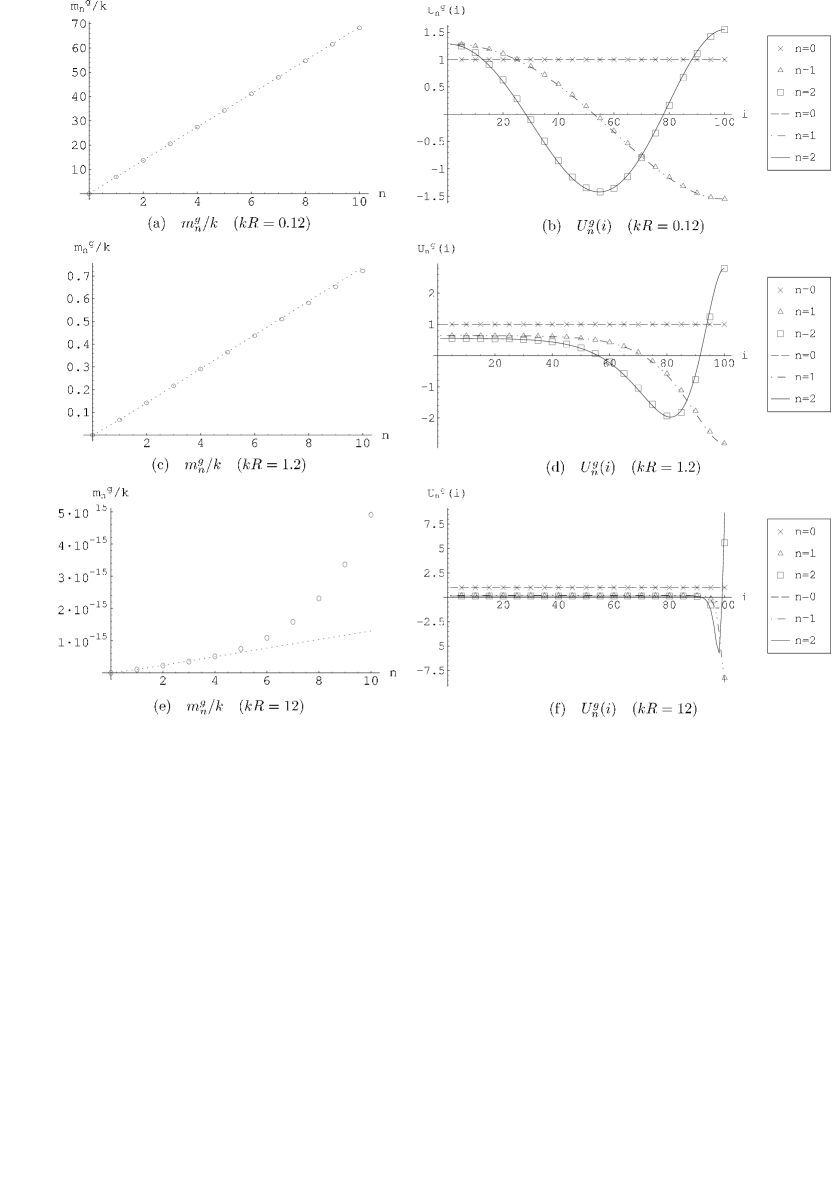
Figure 8.2: Numerical comparison of warped gauge theory and gauge theory in AdS₅. The mass spectra $m_{n}^{g}$ are shown in (a), (c) and (e), and the wave function profiles $U_{n}^{g}(i)$ are shown in (b), (d) and (f) for a vector field in warped gauge theory (depicted by symbols) and gauge theory in AdS₅ (depicted by lines). $n$ labels the index of KK excited mode and $i$ stands for the lattice site or fifth dimension $y=iL/2N$.

8.1.2 Abelian case with nonuniversal gauge couplings

Now let us compare the 4D model with generic couplings to extra dimensional ones. We define the dimensionless parameters $f_{i}$ and $h_{i}$ as [80]

$$g_{i}\,=\,gf_{i},\qquad v_{i}\,=\,vh_{i}.$$ (8.9)

First we restrict ourselves to the case that the gauge group is $U(1)$, namely Abelian theory with no vector self-couplings. Similarly substituting Eq. (8.9) and taking the continuum limit, Eq. (8.2) becomes

$${\cal L}_{gm} = \frac{1}{2}\int_{0}^{L/2}\!dy\,\Bigl{[}h(y)\partial_{y}\bigl{(}f(y)A_{\mu}(x,y)\bigr{)}\Bigr{]}^{2}.$$ (8.10)

Eq. (8.10) induces the kinetic energy term along the extra dimension and mass terms for the vector field on the warped background metric

$$ds^{2}=G_{MN}dx^{M}dx^{N}=(f(y)h(y))^{2}\eta_{\mu\nu}dx^{\mu}dx^{\nu}-dy^{2}.$$ (8.11)

The bulk and boundary mass terms are $y$-dependent and proportional to the derivatives of $f(y)$.

8.1.3 Non-Abelian case with nonuniversal gauge couplings

In the above Abelian case we have discussed that the nonuniversal $f_{i}$ can be interpreted as $y$-dependent bulk/boundary masses in the warped extra dimension. Next we treat the non-Abelian theory with vector self-couplings. Since in this case we also have $y$-dependent vector self-couplings in addition to the $y$-dependent bulk/boundary masses, it may be convenient and instructive to see $f_{i}$ as a $y$-dependent coefficient of the vector kinetic term [80]. To this end, we define the four-dimensional field $A_{5}^{i}$,

$$Q_{i}\equiv v_{i}e^{-ia(g_{i}A_{5}^{i}+g_{i+1}A_{5}^{i+1})/2}=v_{i}\left(1-ia(g_{i}A_{5}^{i}+g_{i+1}A_{5}^{i+1})/2+{\cal O}(a^{2})\right),$$ (8.12)

where $a\equiv L/(2N)$ is the lattice spacing, which goes to zero in the continuum limit. Rescaling the gauge fields $\sqrt{N}f_{i}(A^{i}_{\mu},\,A^{i}_{5})\to(A^{i}_{\mu},\,A^{i}_{5})$, the kinetic term $-\frac{1}{4}\sum_{i=1}^{N}F_{\mu\nu}^{i}F^{i\mu\nu}$ and Eq. (8.1) become

$${\cal L}^{gQ}_{kin} = -\frac{1}{4}\sum_{i=1}^{N}a\frac{f^{-2}_{i}}{L/2}F^{i}_{\mu\nu}F^{i\mu\nu}$$ (8.13)

$$+\sum_{i=1}^{N-1}a\frac{h^{2}_{i}}{L/2}\Bigg{|}\partial_{\mu}A_{5}^{i+\frac{1}{2}}-\frac{A^{i+1}_{\mu}-A^{i}_{\mu}}{a}-i\hat{g}[A^{i}_{\mu},A_{5}^{i+\frac{1}{2}}]$$

$$\qquad\qquad\qquad\qquad\qquad\qquad+i\hat{g}A_{5}^{i+\frac{1}{2}}(A^{i+1}_{\mu}-A^{i}_{\mu})+{\cal O}(a^{1/2})\Bigg{|}^{2},$$

where $\hat{g}=g/\sqrt{N}$ and $A_{5}^{i+\frac{1}{2}}\equiv(A_{5}^{i}+A_{5}^{i+1})/2$. In the continuum limit $N\to\infty$ with $L$ and $\hat{g}$ fixed, Eq. (8.13) results in

$${\cal L}^{gQ}_{kin} = -\frac{1}{4}\int_{0}^{L/2}dy\frac{f^{-2}(y)}{L/2}\Big{[}\eta^{\mu\nu}\eta^{\rho\sigma}F_{\mu\rho}F_{\nu\sigma}-2(h(y)f(y))^{2}\eta^{\mu\nu}F_{\mu 5}F_{\nu 5}\Big{]},$$

where $F_{MN}(x,y)=\partial_{M}A_{N}(x,y)-\partial_{N}A_{M}(x,y)--i\hat{g}[A_{M}(x,y),A_{N}(x,y)]$. This completely reproduces the 5D Yang-Mills kinetic term with a $y$-dependent coefficient

$${\cal L}^{vec}_{warp} = -\frac{1}{4}\int_{0}^{L/2}\!dy\,f^{-2}(y)\sqrt{-G}G^{MN}G^{AB}F_{MA}F_{NB}$$ (8.14)

on the warped-background metric (8.11), provided that $g_{\rm 5D}=\sqrt{L/2}\,\hat{g}$. This is the generic correspondence between the present 4D model and continuum 5D theory. From Eq. (8.14), we thus find the $y$-dependent factor $f^{-2}(y)$ in front of the canonical Yang-Mills term, which corresponds to a 5D dilaton VEV. The factor does carry the origin of the massless vector localization shown in Eq. (8.4). With the constant gauge coupling $g_{i}\equiv g$ ($f_{i}$ = 1), one obtains the bulk vector field with a constant zero mode on the warped metric (8.11). A field redefinition $f^{-1}(y)A_{M}\to A_{M}$ in Eq. (8.14) gives the previous bulk/boundary mass terms but one then has $y$-dependent vector self-couplings in non-Abelian cases.

8.2 Toward dynamical realization

We have shown that the 4D models with nonuniversal VEVs, gauge and other couplings can describe 5D physics on curved backgrounds, including the RS model with the exponential warp factor. In the continuum 5D theory, this factor is derived as a solution of the equation of motion for gravity. On the other hand, in the 4D viewpoint, warped geometries are generated by taking the couplings and VEVs as appropriate forms. In the previous sections, we have just assumed their typical forms and examined its consequences. If one could identify how to control these couplings by underlying dynamics [80], resultant 4D theories turn out to provide attractive schemes to discuss low energy physics such as tiny coupling constants.

8.2.1 Dimensional transmutation in strong coupling

First we consider the scalar VEVs $\langle Q_{i}\rangle=v_{i}$. A simple way to dynamically control them is to introduce additional strongly-coupled gauge theories [82]. Consider the following set of asymptotically free gauge theories:

$$A_{\mu}^{i} : SU(n)_{i}\textrm{ gauge field }(g,\Lambda)$$

$$\hat{A}_{\mu}^{i} : SU(m)_{i}\textrm{ gauge field }(\hat{g}_{i},\hat{\Lambda}_{i}),$$

where $\Lambda$ and $\hat{\Lambda}_{i}$ denote the dynamical scales. We have, for simplicity, assumed the common values of $g$ and $\Lambda$ for all $SU(n)_{i}$. In addition, two types of fermions are introduced

$$\xi^{i}\;:\;(n,\bar{m},1),\qquad\bar{\xi}^{i}\;:\;(1,m,\bar{n}),$$

where their representations under $SU(n)_{i}\times SU(m)_{i}\times SU(n)_{i+1}$ gauge groups are shown in the parentheses. If $\hat{\Lambda}_{i}\gg\Lambda$, the $SU(m)_{i}$ theories confine at a higher scale than $SU(n)_{i}$, and the fermion bilinear composite scalars $Q_{i}\sim\xi^{i}\bar{\xi}^{i}$ appear. Their VEVs $v_{i}$ are given by the dynamical scales $\hat{\Lambda}_{i}$ of the $SU(m)_{i}$ gauge theories through the dimensional transmutation as

$$\langle Q_{i}\rangle\,\equiv\,v_{i}\,\simeq\,\hat{\Lambda}_{i}\,=\,\mu\,e^{\frac{1}{2\hat{\beta}\hat{g}_{i}^{2}(\mu)}},$$ (8.15)

where $\hat{\beta}$ is a universal one-loop gauge beta function for $SU(m)_{i}$ ($\hat{\beta}<0$). The gauge couplings $\hat{g}_{i}$ generally take different values and thus leads to different values of $v_{i}$. For example, a linear dependence of $1/\hat{g}_{i}^{2}$ on the index $i$ is amplified to an exponential behavior of $v_{i}$. That is,

$$\frac{1}{\hat{g}_{i}^{2}(\mu)}\,=\,-2\hat{\beta}\biggl{(}\frac{k}{gv}\biggr{)}i\quad\longleftrightarrow\quad v_{i}\,=\,ve^{-ki/gv},$$

which reproduces bulk fields on the RS background as shown before. Index dependences of gauge couplings are actually generic situations, and may also be controlled, for example, by some mechanism fixing dilatons or a radiatively induced kinetic terms discussed below. A supersymmetric extension of the above scenario is achieved with quantum-deformed moduli spaces [100].

8.2.2 FI terms in supersymmetric warped $U(1)$ gauge theory

Another mechanism which dynamically induces nonuniversal VEVs is obtained in supersymmetric cases [80]. Consider the gauge group $\prod_{i}U(1)_{i}$ and the chiral superfields $Q_{i}$ with charges $(+1,-1)$ under $U(1)_{i}\times U(1)_{i+1}$. It is assumed that the scalar components $q_{i}$ of $Q_{i}$ develop their VEVs $\langle q_{i}\rangle=v_{i}$. The $D$ term of each $U(1)_{i}$ is given by

$$D_{i}\,=\,\epsilon_{i}+|q_{i}|^{2}-|q_{i-1}|^{2}+\cdots,$$ (8.16)

where $\epsilon_{i}$ is the coefficient of the Fayet-Iliopoulos (FI) term, and the ellipsis denotes contributions from other fields charged under $U(1)_{i}$, which are assumed not to have VEVs. Given nonvanishing FI terms, $\epsilon_{i}\neq 0$, the $D$-flatness conditions mean

$$v_{i-1}^{2}\,=\,v_{i}^{2}+\epsilon_{i},$$ (8.17)

and nonuniversal VEVs $v_{i}$ are indeed realized. In this case, a dynamical origin of nonuniversal VEVs is nonvanishing FI terms. These may be generated at loop level. Furthermore, if matter contents are different for each gauge theory, $\epsilon_{i}$ themselves have complicated forms. This supersymmetric warped $U(1)$ gauge theory might reveal the localization nature of 5D $S^{1}/Z_{2}$ orbifold model with generic FI terms on boundaries that was discussed in Chapter 3.

8.3 Discussions: field localization in index space

We have formulated 4D models which provide 5D field theories on generic warped backgrounds. The warped geometries are achieved with generic values of symmetry breaking VEVs, gauge couplings and other couplings in the models. We have focused on field localization behaviors along the index space of gauge theory (the fifth dimension in the continuum limit), which is realized by taking relevant choices of mass parameters.

As a good and simple application, we have constructed 4D models corresponding to bulk field theories on the AdS₅ Randall-Sundrum background. The localized wave-functions of massless modes are completely reproduced with a finite number of gauge groups. In addition, the exponentially suppressed spectrum of KK modes is also generated. These results imply that most properties of brane world models can be obtained within 4D gauge theories. Supersymmetric extensions have also been investigated. In 5D warped models, bulk and boundary mass terms of spinors and scalars satisfy complicated forms imposed by supersymmetry on the RS background. However, we show in our formalism that these forms of mass terms are derived from a 4D global supersymmetric model on the flat background.

The conditions on the model parameters should be explained by some dynamical mechanisms if one considers the models from a fully 4D viewpoint. One of interesting ways is to include additional strongly-coupled gauge theories. In this case, a small ${\cal O}(1)$ difference between gauge couplings is converted to exponential profiles of symmetry breaking VEVs via dimensional transmutation, and indeed generates a warp factor of the RS model. A difference of gauge couplings is achieved by, for example, dynamics controlling dilatons, or radiative corrections to gauge couplings. Supersymmetrizing models provide a mechanism of dynamically realizing nonuniversal VEVs with $D$-flatness conditions.

Our formulation makes sense not only in the 4D points of view but also as lattice-regularized 5D theories. In this sense, such as the AdS/CFT correspondence might be clearly seen with our formalism. As other applications, it can be applied to construct various types of curved backgrounds and bulk/boundary masses. For example, we have discussed massless vector localization by varying the gauge couplings $g_{i}$. Furthermore, one might consider the models in which some fields are charged under only some of gauge groups. That seems not a bulk nor brane fields, but ‘quasi-bulk’ fields. Applications including these phenomena will be studied elsewhere.

Chapter 9 Conclusions and discussions

One of the most important subjects in modern theoretical particle physics is the unification of all fundamental interactions. We know few successful candidates for the theory of quantum gravity. The most promising one is superstring theory defined in ten-dimensional space-time, and we necessarily have extra dimensions to derive standard model in four-dimensional space-time from it. Recent interesting perspective is that various problems in the standard model can be solved in a process of compactifying nontrivially such extra dimensions, e.g., with orbifolding or with D-branes (orientifolding). In this thesis we notice such aspect, and investigate the structure of spontaneous or dynamical symmetry breaking in the bulk and boundary system as a general and most simple approximation of the effective theory.

In Part I we studied spontaneous supersymmetry breaking and its communication from the hidden to visible sector in the system. The low scale supersymmetry breaking picture preferably merges into the bulk and boundary system because we can sequester the supersymmetry breaking (hidden) sector by utilizing the branes and spatiality between them in extra dimensions. We reviewed that the $F$ term supersymmetry breaking contribution can be mediated to visible sector through various mechanisms like gravity, gauge, anomaly, gaugino, Kaluza-Klein and radion mediation. We obtained soft breaking parameters in the visible sector caused by each mechanisms. This is useful for understanding low energy phenomenology such as sparticle flavor structure under the supersymmetry breaking.

In a case that local $U(1)$ symmetry with (nonintegrable) FI term exists in the brane world models, we have seen that both the field localization effect and the $D$ term supersymmetry breaking contributions also play important roles in low energy [41]. For instance, if the $U(1)$ symmetry gives different charge per generation, a nontrivial VEV of the gauge scalar field induces different localization profile in extra dimension depending on the charge. That may cause a hierarchical structure in the Yukawa coupling, in addition to the contribution from the Froggatt-Nielsen mechanism. And if the charge is different between quarks and leptons, the proton decay may be suppressed by such localization. At the same time, with such localization effects, we have $D$ term contribution to the soft scalar masses which is universal everywhere in bulk up to $U(1)$ charge, and may affect the low energy physics.

If the supersymmetry is broken with higher energy scale, we need another mechanism to stabilize electroweak Higgs mass scale. We have such a candidate that electroweak symmetry is broken by fermion bilinear condensation, that is a composite Higgs scenario. For such scenario we need strong binding forces between fermion and anti-fermion to cause such a condensation. The gauge theory with compact extra dimensions may give such strong forces caused by KK gauge bosons. We have studied in detail the dynamics of such gauge theory with matters on boundaries [57, 58, 59, 60]. We have analyzed dynamical fermion masses on a boundary and a decay constant of fermion bilinear operator [57] by using the improved ladder Schwinger-Dyson equation and the Pagels-Stoker formula. We obtain usual 4D Yang-Mills type or gauged NJL type strong dynamics from the bulk gauge theory, depending on the structure of the bulk and the boundary configuration, i.e., the position of the brane, the number of extra dimensions and its curvature. The dynamical mass scale, induced on the boundaries by the former Yang-Mills type and the latter NJL type dynamics, is usual dimensional transmutational scale $\Lambda_{\rm QCD}$ and a reduced scale from bulk fundamental scale, respectively. The reduced scale is warp suppressed on $y^{\ast}=\pi R$ brane in warped brane world and in this case the dynamical mass scale can be electroweak scale, though the fundamental scale in the bulk is near the Planck scale. This is, in a sense, dynamical realization of so called Randall-Sundrum scenario.

These results are important for applying our system to phenomenological models such as top mode SM. In this thesis we suggest a possibility to realize a simple primary model of top quark condensation in RS brane world that is summarized in Fig. 7.14. Our analysis here might be useful to construct any other dynamical models in the bulk and boundary system. Also in a theoretical sense it is concluded that theories in the bulk and boundary system have a nontrivial and interesting vacuum structure and/or a nonperturbative dynamics. Technically it remains as a future work that we analyze the system adopting another way of gauge fixing in order to satisfy Ward-Takahashi identity in more accuracy than one utilized in this thesis. It is because the slight violation of the identity, namely the shift of the value of wave function renormalization factor $A(x)$ from $1$, also deviates a bit the value of the dynamical mass function $B(x)$ from the correct one. This may be done with nonlocal gauge fixing formulated in appendix D.2.

In both SUSY and nonSUSY case it is understood that the wave function localization in extra dimensions gives important effects on the spontaneous or dynamical symmetry breaking in the bulk and boundary system. Such nontrivial field profiles that lead to the hierarchical couplings, strong-weak phase splitting in extra dimensions are generated by some boundary terms, e.g., FI terms and curvature effects of extra dimensions. This can be the geometrical origin of the hierarchical structures between parameters in SM. We have also studied one of the regularization of higher-dimensional theory in order to obtain a renormalizable theory. We formulated warped gauge theory as the regularized theory, and showed that field localization is realized in the index space of the product gauge group [80]. By using warped gauge theory, we obtain more predictive results from the bulk and boundary theories. Inversely, in the warped gauge theory, we understand that we need fine-tuned couplings in four-dimensional theory to realize, in a purely four-dimensional framework, the same nontrivial results as in the higher-dimensional theories. In this sense, we can say that the higher-dimensional theories have more rich structure than the four-dimensional ones.

Phenomenologically interesting features investigated in this thesis are based on the nontrivial compactification of the higher-dimensional field theory. So the future task is to check that such interesting models can be derived from the compactification of just superstring theory. It may be interesting to reanalyze the orbifold compactification of heterotic string, D-branes in type I superstring, and their intersection [4] in terms of such phenomenological sense.

Acknowledgements

First I would like to thank Profs. Taichiro Kugo (Kyoto U.), Taizo Muta (Hiroshima U.) and Masanori Okawa (Hiroshima U.) very much for their hospitality as my supervisors.

I greatly thank Tomohiro Inagaki (Hiroshima U.) and Tatsuo Kobayashi (Kyoto U.) for many precious discussions and important comments, especially during our collaboration.

I would also like to thank Kenji Fukazawa (Kure N. C. T.), Michio Hashimoto (KEK), Tetsutaro Higaki (Kyoto U.), Yasuhiko Katsuki (Kure U.), Nobuhito Maru (U. of Tokyo), Hironori Miguchi (SONY LSI, Fukuoka), Seiji Mukaigawa (Iwate U.), Hiroaki Nakano (Niigata U.), Kensaku Ohkura (Hiroshima U.), Masaharu Tanabashi (Tohoku U.) and Koichi Yoshioka (Kyushu U.) for fruitful discussions and correspondences.

I thank all of the other members in theoretical particle physics groups in Hiroshima and Kyoto university for their hospitality and encouraging me.

Appendix A Wave-function renormalization and soft parameters

We can determine soft terms of an observable field via its wave function renormalization if the supersymmetry breaking is communicated by perturbatively renormalizable interactions. That means that we can obtain all the information about the soft terms from an anomalous dimension and a beta function. For example, we should calculate one-loop and two-loop diagrams to obtain the form of a gaugino and a sfermion soft mass respectively in the minimal gauge-mediated scenario. It is, however, easier to determine anomalous dimensions and beta functions than such loop calculations. In this appendix we review the calculus how to determine soft parameters from the wave function renormalization following G. F. Giudice and R. Rattazzi [24].

For such purpose we are interested in the case that the supersymmetry-breaking scale and the mediation scale are completely determined by the VEVs of a scalar and an auxiliary component of a chiral superfield $X$:

$$\langle X\rangle=M+\theta^{2}F$$

In a conventional gauge-mediated scenario a messenger field receives a mass via a superpotential $X\bar{\Phi}\Phi$. In the case $F\ll M^{2}$ supersymmetry is broken only by the soft terms below the messenger scale, and we can utilize explicitly supersymmetric formulation to chase the supersymmetry breaking effects.

Thanks to the nonrenormalization theorem of the superpotential the gaugino and the sfermion masses are generated by $X$-dependent renormalization of the kinetic terms (wave-function) of them. That is, only the gauge coupling $g^{2}$ and the matter wave function renormalization $Z_{i}$ is the source of the soft masses. Therefore in the case with only one (spurion) field $X$, we calculate $g^{2}$ and $Z_{i}$ in the supersymmetric limit $X=M$ ($M$ is a c-number), and then we replace $M$ with the superfield $X$ in the final results. This is the most important point, however, we should note that for $Z_{i}(M,\mu)$ the replacement which is consistent with a chiral reparameterization $X\to e^{i\phi}X$ is $M\to\sqrt{X^{\dagger}X}$, while $M\to X$ should be performed for the gauge coupling $g^{2}(M,\mu)$.

Gaugino mass

The gaugino mass renormalized at scale $\mu$ is extracted from the $X$-dependent wave function renormalization:

$${\cal L}=\int d^{2}\theta\,S(X)W^{a\alpha}W^{a}_{\alpha}+{\rm h.c.},$$ (A.1)

where $S(X)$ is expanded around $\theta,\bar{\theta}=0$ as

$$S(X) = S(X(0,0))+\left(\theta\frac{\partial}{\partial\theta}+\bar{\theta}\frac{\partial}{\partial\bar{\theta}}\right)S(X(0,0))+\frac{1}{2!}\left(\theta\frac{\partial}{\partial\theta}+\bar{\theta}\frac{\partial}{\partial\bar{\theta}}\right)^{2}S(X(0,0))+\ldots$$ (A.2)

$$= \left[S+\frac{1}{2}\frac{\partial S}{\partial X}\frac{\partial X}{\partial(\theta^{2})}\theta^{2}+(\theta,\ \bar{\theta},\ \bar{\theta}^{2},\ \theta^{2}\bar{\theta}^{2}{\rm term})\right]_{X=X(0,0)=M}$$

$$= S(M)\left[1+\frac{1}{2}\frac{1}{S}\frac{\partial S}{\partial X}\frac{\partial X}{\partial(\theta^{2})}\theta^{2}+(\theta,\ \bar{\theta},\ \bar{\theta}^{2},\ \theta^{2}\bar{\theta}^{2}{\rm term})\right]_{X=M}.$$

Canonically normalizing the gaugino kinetic term in (A.1) and using $\partial X/\partial(\theta^{2})=F$, we obtain the gaugino mass in the form

$$\bar{M}_{g}(\mu) = -\frac{1}{2}\left.\frac{1}{S}\frac{\partial S}{\partial X}\right|_{X=M}\!\!\!F\quad=-\frac{1}{2}\left.\frac{1}{X}\frac{\partial\ln S(X,\mu)}{\ln X}\right|_{X=M}F.$$ (A.3)

Then we know that we can calculate gaugino mass from a function $S(X)$. Because the scalar component $S(M,\mu)$ of $S(X)$ is a coefficient function of the gauge kinetic term, we can determine it:

$$S(M,\mu)=\frac{\alpha^{-1}(M,\mu)}{16\pi}-\frac{i\Theta}{32\pi^{2}},$$

where $\alpha=g^{2}/4\pi$ is a gauge coupling and $\Theta$ is a topological vacuum angle.

The function $\alpha(M,\mu)$ is given by integrating the renormalization group (RG) evolution from the ultra-violet (UV) scale $\Lambda_{\rm UV}$ to the observation scale $\mu$ over the messenger threshold $M$. From the one-loop RG equation we find

$$\frac{d}{dt}\alpha^{-1}=\frac{b}{2\pi}\qquad(t=\ln\mu),$$ (A.4)

where the beta-function coefficient $b$ is given by $b=3N_{c}-N_{f}$ for the $SU(N_{c})$ gauge theory with $N_{f}$ flavor. Above the messenger scale $M$ the running of the gauge coupling suffers from messenger fields $\Phi_{i}$ and $\bar{\Phi}_{i}$ ($i=1,\ldots,N$), which transforms as $N_{c}+\bar{N}_{c}$ of $SU(N_{c})$, and the beta-function coefficient becomes $b^{\prime}=b-N$. Therefore the one-loop running of the gauge coupling is given by

$${\rm Re}S(M,\mu) = \frac{\alpha^{-1}(M,\mu)}{16\pi}$$ (A.5)

$$= \frac{\alpha^{-1}(\Lambda_{\rm UV},\Lambda_{\rm UV})}{16\pi}+\frac{b^{\prime}}{32\pi^{2}}\ln\frac{|M|}{\Lambda_{\rm UV}}+\frac{b}{32\pi^{2}}\ln\frac{\mu}{|M|}.$$

This equation and the holomorphic property determines the form of $S(X,\mu)$. In this equation we replace $M$ as $M\to X$ and obtain

$$S(X,\mu) = S(\Lambda_{\rm UV},\Lambda_{\rm UV})+\frac{b^{\prime}}{32\pi^{2}}\ln\frac{X}{\Lambda_{\rm UV}}+\frac{b}{32\pi^{2}}\ln\frac{\mu}{X}.$$ (A.6)

The imaginary part of this equation reproduces renormalization $\Theta\to(b-b^{\prime})\arg(X)$ that shows the chiral anomaly.

By differentiating Eq. (A.6) by $\ln X$ for fixed $S(\Lambda_{\rm UV})$ we finally obtain the form of the gaugino mass

$$\bar{M}_{g}(\mu) = -\frac{1}{2}\left.\frac{1}{S(X,\mu)}\frac{b^{\prime}-b}{32\pi^{2}}\frac{F}{X}\right|_{X=M}$$ (A.7)

$$= -\frac{1}{2}16\pi\,\alpha(M,\mu)\,\frac{-N}{32\pi}\frac{F}{M}$$

$$= \frac{\alpha(\mu)}{4\pi}N\frac{F}{M}.$$

This agrees with the result from the direct loop integration of some diagrams.

Sfermion mass

We also define the wave function renormalization $Z_{Q}$ of a chiral superfield $Q$ by

$${\cal L}=\int d^{4}\theta Z_{Q}(X,X^{\dagger})Q^{\dagger}Q.$$ (A.8)

Different from the gaugino case here we should take account of $D$ term renormalization and $Z_{Q}$ is real and is a function of both $X$ and $X^{\dagger}$.

We expand $Z_{Q}$ around $\theta^{2},\bar{\theta}^{2}=0$ as

$$Z_{Q}(X(\theta,\bar{\theta}),X^{\dagger}(\theta,\bar{\theta}))$$ (A.9)

$$= Z_{Q}(X(0,0),X^{\dagger}(0,0))+\frac{\partial Z_{Q}(X(0,0),X^{\dagger}(0,0))}{\partial X}F\theta^{2}$$

$$+\frac{\partial Z_{Q}(X(0,0),X^{\dagger}(0,0))}{\partial X^{\dagger}}F^{\dagger}\bar{\theta}^{2}+\frac{\partial^{2}Z_{Q}(X(0,0),X^{\dagger}(0,0))}{\partial X\partial X^{\dagger}}FF^{\dagger}\theta^{2}\bar{\theta}^{2}$$

$$= \left[Z_{Q}+\frac{\partial Z_{Q}}{\partial X}F\theta^{2}+\frac{\partial Z_{Q}}{\partial X^{\dagger}}F^{\dagger}\bar{\theta}^{2}+\frac{\partial^{2}Z_{Q}}{\partial X\partial X^{\dagger}}FF^{\dagger}\theta^{2}\bar{\theta}^{2}\right]_{\tiny\matrix{X=X(0,0)=M\cr X^{\dagger}=X^{\dagger}(0,0)=M^{\dagger}}}$$

$$= \left[Z_{Q}\left(1+\frac{\partial\ln Z_{Q}}{\partial X}F\theta^{2}+\frac{\partial\ln Z_{Q}}{\partial X^{\dagger}}F^{\dagger}\bar{\theta}^{2}+\frac{1}{Z_{Q}}\frac{\partial^{2}Z_{Q}}{\partial X\partial X^{\dagger}}FF^{\dagger}\theta^{2}\bar{\theta}^{2}\right)\right]_{\tiny\matrix{X=M\cr X^{\dagger}=M^{\dagger}}}$$

$$= \left[Z_{Q}\left\{\left(1+\frac{\partial\ln Z_{Q}}{\partial X}F\theta^{2}\right)^{\dagger}\left(1+\frac{\partial\ln Z_{Q}}{\partial X}F\theta^{2}\right)+\frac{1}{X^{\dagger}X}\frac{\partial\ln Z_{Q}}{\partial\ln X\partial\ln X^{\dagger}}FF^{\dagger}\theta^{2}\bar{\theta}^{2}\right\}\right]_{\tiny\matrix{X=M\cr X^{\dagger}=M^{\dagger}}}$$

$$= \left[Z_{Q}\left(1+\frac{\partial\ln Z_{Q}}{\partial X}F\theta^{2}\right)^{\dagger}\left(1+\frac{\partial\ln Z_{Q}}{\partial X}F\theta^{2}\right)\left\{1+\frac{\frac{1}{X^{\dagger}X}\frac{\partial\ln Z_{Q}}{\partial\ln X\partial\ln X^{\dagger}}FF^{\dagger}\theta^{2}\bar{\theta}^{2}}{\left(1+\frac{\partial\ln Z_{Q}}{\partial X}F\theta^{2}\right)^{\dagger}\left(1+\frac{\partial\ln Z_{Q}}{\partial X}F\theta^{2}\right)}\right\}\right]_{\tiny\matrix{X=M\cr X^{\dagger}=M^{\dagger}}}.$$

In Eq. (A.8) we canonically normalize the matter superfield

$${\cal Z}Q\equiv\left.\sqrt{Z_{Q}}\left(1+\frac{\partial\ln Z_{Q}}{\partial X}F\theta^{2}\right)\right|_{\tiny\matrix{\ \cr X=M\cr X^{\dagger}=M^{\dagger}}}Q\qquad\quad\to Q$$ (A.10)

and the mass of a scalar component of $Q$ results in

$$\tilde{m}_{Q}^{2}(\mu) = -\left.\left[\frac{\frac{1}{X^{\dagger}X}\frac{\partial\ln Z_{Q}}{\partial\ln X\partial\ln X^{\dagger}}FF^{\dagger}\theta^{2}\bar{\theta}^{2}}{\left(1+\frac{\partial\ln Z_{Q}}{\partial X}F\theta^{2}\right)^{\dagger}\left(1+\frac{\partial\ln Z_{Q}}{\partial X}F\theta^{2}\right)}\right]_{D}\right|_{\tiny\matrix{X=M\cr X^{\dagger}=M^{\dagger}}}$$ (A.11)

$$= -\left.\frac{1}{X^{\dagger}X}\frac{\partial\ln Z_{Q}}{\partial\ln X\partial\ln X^{\dagger}}FF^{\dagger}\right|_{\tiny\matrix{X=M\cr X^{\dagger}=M^{\dagger}}}$$

$$= -\left.\frac{\partial\ln Z_{Q}(X,X^{\dagger},\mu)}{\partial\ln X\partial\ln X^{\dagger}}\right|_{\tiny\matrix{X=M\cr X^{\dagger}=M^{\dagger}}}\frac{FF^{\dagger}}{MM^{\dagger}}.$$

By following the similar way we can obtain a corresponding formula of $A$ term.

The one-loop wave function renormalization of the chiral superfield $Q$ is given by

$$\frac{d}{dt}\ln Z_{Q}=\frac{c}{\pi}\alpha,$$ (A.12)

where $c$ is the second Casimir of the gauge group that is given by $c=(N^{2}-1)/2N$ for $SU(N)$ fundamental representation. The function $Z_{Q}(M,\mu)$ is determined by integrating Eq. (A.12) from $\Lambda_{\rm UV}$ to $\mu$ and matching it at the threshold $M$ with the tree level one. Namely,

$$Z_{Q}(X,X^{\dagger},\mu)=Z_{Q}(\Lambda_{\rm UV})\left[\frac{\alpha(\Lambda_{\rm UV})}{\alpha(X)}\right]^{2c/b^{\prime}}\left[\frac{\alpha(X)}{\alpha(\mu)}\right]^{2c/b},$$ (A.13)

where we define

$$\alpha^{-1}(\mu) \equiv 16\pi{\rm Re}S(\sqrt{XX^{\dagger}},\mu)\ =\ \alpha^{-1}(X)+\frac{b}{4\pi}\ln\frac{\mu^{2}}{XX^{\dagger}}$$

$$\alpha^{-1}(X) \equiv 16\pi{\rm Re}S(\sqrt{XX^{\dagger}},\sqrt{XX^{\dagger}})\ =\ \alpha^{-1}(\Lambda_{\rm UV})+\frac{b^{\prime}}{4\pi}\ln\frac{XX^{\dagger}}{\Lambda_{\rm UV}^{2}},$$ (A.14)

by performing $M\to\sqrt{XX^{\dagger}}$ in the function $S(M,\mu)$ in Eq. (A.5). We note that $\alpha$, i.e., the real part of $S(X,\mu)$ is nonchiral though $S(X,\mu)$ is chiral.

By differentiating Eq. (A.11) by $X$ for fixed UV parameters $Z_{Q}(\Lambda_{\rm UV})$ and $\alpha(\Lambda_{\rm UV})$, we obtain the soft parameters:

$$\tilde{m}_{Q}^{2}(\mu) = 2c\frac{\alpha^{2}(\mu)}{(4\pi^{2})}N\left[\xi^{2}+\frac{N}{b}(1-\xi^{2})\right]\left(\frac{F}{M}\right)^{2}$$ (A.15)

$$A_{i}(\mu) = \frac{2c_{i}}{b}\frac{\alpha(\mu)}{4\pi}N(\xi-1)\frac{F}{M}$$ (A.16)

$$\xi \equiv \frac{\alpha(M)}{\alpha(\mu)}=\left[1+\frac{b}{2\pi}\alpha(\mu)\ln\frac{M}{\mu}\right]^{-1}.$$

These coincide with the well-known soft terms given by taking the effect of leading-log in the gauge-mediated scenario.

Appendix B SUSY formula in 5D $S^{1}/Z_{2}$

In this appendix we review a formula of off-shell supersymmetric vector and hyper multiplets in 5D following Ref. [35]. We neglect the gravity (Weyl) multiplet.

B.1 Symplectic reality condition

Here we consider one vector multiplet $V=\{A_{M},\lambda_{i},\Sigma,\vec{D}\cdot\vec{\sigma}_{ij}\}$ and a set of hyper multiplets $H^{\alpha}=\{\Phi_{i}^{\,\alpha},\Psi^{\alpha},F_{i}^{\,\alpha}\}$ where $i,j=1,2$ are $SU(2)_{R}$ indices and $\alpha=1,\ldots,2n$. $\lambda_{i}$ and $\Psi^{\alpha}$ are $USp(2)$ and $USp(2n)$ Majorana spinors, respectively with reality conditions,

$$\lambda_{i}=\varepsilon_{i}^{\,j}\lambda^{C}_{j},\quad\Psi^{\alpha}=({\mathbf{1}}\otimes\varepsilon)^{\alpha}_{\,\beta}(\Psi^{\beta})^{C},$$ (B.1)

where $\varepsilon=\left(\begin{array}[]{cc}0&1\cr-1&0\end{array}\right)$, ${\mathbf{1}}\otimes\varepsilon=\left(\begin{array}[]{cc}0&{\mathbf{1}}_{n}\cr-{\mathbf{1}}_{n}&0\end{array}\right)$, $\Psi^{C}\equiv C\bar{\Psi}^{T}$, and the charge conjugation matrix $C$ is defined as

$$C^{-1}\gamma^{M}C=(\gamma^{M})^{T},\quad C^{T}=-C,\quad C^{\dagger}=C^{-1}.$$

$\Phi_{i}^{\,\alpha}$ also satisfies symplectic reality condition,

$$\Phi^{\,\alpha}_{i}=({\mathbf{1}}\otimes\varepsilon)^{\alpha}_{\,\beta}\Phi^{\,\beta}_{j}(\varepsilon^{-1})^{\,j}_{i}.$$ (B.2)

B.2 Lagrangian and SUSY transformation

The Lagrangian is given by

$${\cal L} = {\cal L}_{V}+{\cal L}_{H},$$

$${\cal L}_{V} = {\rm tr}\left[-\frac{1}{4}F_{MN}F^{MN}+\frac{1}{2}(\partial_{M}\Sigma)^{2}+\frac{1}{2}(\vec{D}\cdot\vec{\sigma}_{ij})^{2}+i\bar{\lambda}_{i}\gamma^{M}D_{M}\lambda^{i}\right],$$

$${\cal L}_{H} = \frac{1}{2}|D_{M}\Phi_{i}^{\,\alpha}|^{2}+\frac{1}{2}|F_{i}^{\,\alpha}|^{2}-\frac{1}{2}g^{2}\Sigma_{a}\Sigma_{b}\Phi_{i}^{\,\alpha\dagger}(t^{a}t^{b})_{\alpha\beta}\Phi^{i\beta}-\frac{1}{2}g\Phi_{i}^{\,\alpha\dagger}(t^{a})_{\alpha\beta}\Phi_{j}^{\,\beta}\vec{D}_{a}\cdot\vec{\sigma}^{ji}$$

$$+\frac{i}{2}\bar{\Psi}^{\alpha}\gamma^{M}D_{M}\Psi_{\alpha}+\frac{1}{2}g\Sigma_{a}\bar{\Psi}^{\alpha}(t^{a})_{\alpha\beta}\Psi^{\beta}+2g\bar{\Psi}^{\alpha}(t^{a})_{\alpha\beta}\Phi^{\beta}_{i}\lambda^{i}_{a},$$

where $D_{M}=\partial_{M}+igA_{M}^{a}t^{a}$ is a covariant derivative, $(t^{a})_{\alpha\beta}\equiv-(T^{a}\otimes\sigma_{3})_{\alpha\beta}=\left(\begin{array}[]{cc}-T^{a}&0\\ 0&T^{a}\end{array}\right)_{\alpha\beta}$, and $T^{a}$ is a generator of the gauge group. This Lagrangian is invariant under the (global) SUSY transformation,

$$\left\{\begin{array}[]{rcl}\delta A_{M}&=&i\bar{\epsilon}^{i}\gamma_{M}\lambda_{i},\\ \delta\lambda_{i}&=&F^{MN}\gamma_{MN}\epsilon_{i}/4-\gamma^{M}\partial_{M}\Sigma\epsilon_{i}/2-i\vec{\sigma}_{i}^{\,j}\cdot\vec{D}\epsilon_{j}/2,\\ \delta\Sigma&=&i\bar{\epsilon}^{i}\lambda_{i},\\ \delta\vec{D}&=&\bar{\epsilon}_{i}\vec{\sigma}^{ij}\gamma^{M}\partial_{M}\lambda_{j},\end{array}\right.$$ (B.4)

$$\left\{\begin{array}[]{rcl}\delta\Phi_{i}^{\alpha}&=&i\bar{\epsilon}_{i}\Psi^{\alpha},\\ \delta\Psi^{\alpha}&=&-\gamma^{M}D_{M}\Phi_{i}^{\alpha}\epsilon^{i}-F_{i}^{\alpha}\epsilon^{i}-ig\Sigma(T^{a})^{\alpha}_{\ \beta}\Phi_{i}^{\beta}\epsilon^{i}\\ \delta F_{i}^{\alpha}&=&i\bar{\epsilon}_{i}\gamma^{M}D_{M}\Psi^{\alpha}+2g\bar{\epsilon}_{j}(T^{a})^{\alpha}_{\,\beta}\Phi^{j\beta}\lambda_{i}^{a}+\bar{\epsilon}_{i}\Sigma_{a}(T^{a})^{\alpha}_{\,\beta}\Psi^{\beta}\end{array}\right.$$ (B.8)

where $\epsilon_{i}$ is a SUSY transformation parameter satisfying a $USp(2)$ Majorana condition $\epsilon_{i}=\varepsilon_{i}^{\,j}\epsilon_{j}^{C}$.

B.3 Orbifold condition

In order to obtain 4D ${\cal N}=1$ SUSY, we perform $S^{1}/Z_{2}$ orbifolding,

$$\epsilon_{i}=\epsilon_{i}(y)=\epsilon_{i}(-y)=(\sigma_{3})_{i}^{\,j}i\gamma^{5}\epsilon_{j}(y)=(\sigma_{3})_{i}^{\,j}i\gamma^{5}\epsilon_{j},\quad i\gamma^{5}=\left(\begin{array}[]{cc}{\mathbf{1}}&0\\ 0&-{\mathbf{1}}\end{array}\right).$$ (B.11)

In addition we require that the gauge symmetry is not broken. Then we have

$$\left\{\begin{array}[]{rcl}\lambda_{i}(-y)&=&(\sigma_{3})_{i}^{\,j}i\gamma^{5}\lambda_{j}(y),\\ \Sigma(-y)&=&-\Sigma(y),\\ \vec{\sigma}_{ij}\cdot\vec{D}(-y)&=&(\sigma_{3}T^{a})\vec{\sigma}_{i}^{\,k}\cdot\vec{D}_{a}(y)(\sigma_{3})_{kj},\end{array}\right.$$ (B.15)

$$\left\{\begin{array}[]{rcl}\Phi_{i}^{\,\alpha}(-y)&=&-({\mathbf{1}}\otimes\sigma_{3})^{\alpha}_{\,\beta}\Phi_{j}^{\,\beta}(y)(\sigma_{3})^{j}_{\,i},\\ \Psi^{\alpha}(-y)&=&({\mathbf{1}}\otimes\sigma_{3})^{\alpha}_{\,\beta}i\gamma^{5}\Psi^{\beta}(y),\\ F_{i}^{\,\alpha}(-y)&=&({\mathbf{1}}\otimes\sigma_{3})^{\alpha}_{\,\beta}F_{j}^{\,\beta}(y)(\sigma_{3})^{j}_{\,i},\end{array}\right.$$ (B.19)

These orbifold condition (B.11)-(B.19) and reality conditions (B.1)-(B.2) are solved simultaneously and result in

$$\epsilon_{i}=\left(\begin{array}[]{c}\epsilon\\ -\epsilon^{C}\end{array}\right),\quad\lambda_{i}=\left(\begin{array}[]{c}\lambda\\ -\lambda^{C}\end{array}\right),$$ (B.24)

$$(\Phi_{i}^{\,\bar{\alpha}}|\Phi_{i}^{\,\bar{\alpha}+n}) = \left(\begin{array}[]{c|c}(\Phi_{-}^{\,\bar{\alpha}})^{*}&\Phi_{+}^{\,\bar{\alpha}}\\ -(\Phi_{+}^{\,\bar{\alpha}})^{*}&\Phi_{-}^{\,\bar{\alpha}}\end{array}\right),$$ (B.27)

$$(\Psi^{\bar{\alpha}}|\Psi^{\bar{\alpha}+n}) = (\Psi^{\bar{\alpha}}|-(\Psi^{\bar{\alpha}})^{C}),$$

$$(F_{i}^{\,\bar{\alpha}}|F_{i}^{\,\bar{\alpha}+n}) = \left(\begin{array}[]{c|c}F_{+}^{\,\bar{\alpha}}&-(F_{-}^{\,\bar{\alpha}})^{*}\\ F_{-}^{\,\bar{\alpha}}&(F_{+}^{\,\bar{\alpha}})^{*}\end{array}\right),$$ (B.30)

where the row of the matrices corresponds to the $SU(2)_{R}$ index $i$, $\epsilon=\epsilon_{+L}-\epsilon_{-R}$, $\epsilon^{C}=\epsilon_{+R}+\epsilon_{-L}$, $\lambda=\lambda_{+L}-\lambda_{-R}$, $\lambda^{C}=\lambda_{+R}+\lambda_{-L}$, $\Psi^{\bar{\alpha}}=\Psi^{\bar{\alpha}}_{+L}-\Psi^{\bar{\alpha}}_{-R}$, $(\Psi^{\bar{\alpha}})^{C}=\Psi^{\bar{\alpha}}_{+R}+\Psi^{\bar{\alpha}}_{-L}$, the subscript $\pm$ represents the eigenvalues of the parity operator $\sigma_{3}i\gamma^{5}$, and $\bar{\alpha}=1,\ldots,n$. The parities of all the independent fields are summarized as follows:

$$V:~{}\begin{array}[]{l|c|c|c|c|c|c|c|}\mbox{state}&A_{\mu}&A_{5}&\Sigma&\lambda_{\pm L}&\lambda_{\pm R}&D_{3}&D_{1,2}\\ \hline\cr\mbox{parity}&+&-&-&\pm&\pm&+&-\end{array}\,,$$

$$\Phi:~{}\begin{array}[]{l|c|c|c|c|}\mbox{state}&\Phi_{\pm}&\Psi_{\pm L}&\Psi_{\pm R}&F_{\pm}\\ \hline\cr\mbox{parity}&\pm&\pm&\pm&\pm\end{array}\,.$$

The SUSY transformations of even components are in the form of

$$\left\{\begin{array}[]{rcl}\delta A_{\mu}&=&i\bar{\epsilon}_{+}\gamma_{\mu}\lambda_{+},\\ \delta\lambda_{+}&=&F^{\mu\nu}\gamma_{\mu\nu}\epsilon_{+}/4-i\widetilde{D_{3}}\epsilon_{+}/2,\\ \delta\widetilde{D_{3}}&=&\bar{\epsilon}_{+}\gamma^{\mu}\partial_{\mu}\lambda_{+},\end{array}\right.$$ (B.34)

$$\left\{\begin{array}[]{rcl}\delta\Phi_{+}^{\bar{\alpha}}&=&i\bar{\epsilon}_{+R}\Psi_{+L}^{\bar{\alpha}},\\ \delta\Psi_{+L}^{\bar{\alpha}}&=&-\gamma^{\mu}D_{\mu}\Phi_{+}^{\bar{\alpha}}\epsilon_{+R}-\widetilde{F}_{+}^{\bar{\alpha}}\epsilon_{+L},\\ \delta\widetilde{F}_{+}^{\bar{\alpha}}&=&\bar{\epsilon}_{+L}(i\gamma^{\mu}D_{\mu}\Psi_{+L}^{\bar{\alpha}}+2g(T^{a})^{\bar{\alpha}}_{\,\bar{\beta}}\Phi_{+}^{\,\bar{\beta}}\lambda_{+R,a}),\end{array}\right.$$ (B.38)

where $D_{\mu}=\partial_{\mu}+igA_{\mu}^{a}T^{a}$, $\widetilde{D_{3}}=D_{3}-\partial_{y}\Sigma$ and $\widetilde{F}_{+}=F_{+}-\partial_{y}\Phi_{-}^{*}$. Now we see that, in the 4D ${\cal N}=1$ language, we have a massless vector multiplet $\widetilde{V}=\{A_{\mu},\lambda_{+},\widetilde{D_{3}}\}$ and chiral multiplets $\Phi_{+}^{\bar{\alpha}}=\{\Phi_{+}^{\bar{\alpha}},\Psi_{+L}^{\bar{\alpha}},\widetilde{F}_{+}^{\bar{\alpha}}\}$.

B.4 Bulk and boundary coupling

So the SUSY is 4D ${\cal N}=1$ because of the above orbifolding, we can also write down the coupling between the above bulk multiplets and some 4D boundary multiplets. We introduce chiral multiplets, $\phi_{0}^{\,\bar{\alpha}_{0}}=\{\phi_{0}^{\,\bar{\alpha}_{0}},\psi_{0L}^{\,\bar{\alpha}_{0}},f_{0}^{\,\bar{\alpha}_{0}}\}$ and $\phi_{\pi}^{\,\bar{\alpha}_{\pi}}=\{\phi_{\pi}^{\,\bar{\alpha}_{\pi}},\psi_{\pi L}^{\,\bar{\alpha}_{\pi}},f_{\pi}^{\,\bar{\alpha}_{\pi}}\}$, on both boundary-fixed planes of $S^{1}/Z_{2}$ orbifold, where $\bar{\alpha}_{0}=1,\ldots,n_{0}$ and $\bar{\alpha}_{\pi}=1,\ldots,n_{\pi}$. These chiral multiplets obey the same SUSY transformation rules as the above $\Phi_{+}$. Then the bulk and boundary coupling can be written as

$${\cal L}_{\rm boundary} = \sum_{I=0,\pi}\delta(y-IR)\Bigg{[}D_{\mu}\phi_{I}^{\,\bar{\alpha}_{I}\dagger}D^{\mu}\phi_{I\bar{\alpha}_{I}}+i\bar{\psi}_{IL}^{\,\bar{\alpha}_{I}}D\!\!\!\!/\psi_{IL\bar{\alpha}_{I}}+f_{I}^{\,\bar{\alpha}_{I}\dagger}f_{I\bar{\alpha}_{I}}$$

$$-g\phi_{I}^{\,\bar{\alpha}_{I}\dagger}(T^{a})_{\bar{\alpha}_{I}\bar{\beta}_{I}}\phi_{I}^{\,\bar{\beta}_{I}}\widetilde{D_{3}}_{,a}-2g\left(\bar{\psi}_{IL}^{\,\bar{\alpha}_{I}}\lambda_{+R,a}(T^{a})_{\bar{\alpha}_{I}\bar{\beta}_{I}}\phi_{I}^{\,\bar{\beta}_{I}}+{\rm h.c.}\right)\Bigg{]}$$

B.5 Abelian vector multiplet

If the gauge symmetry is $U(1)$, the Fayet-Iliopoulos term is invariant under the gauge symmetry and 4D ${\cal N}=1$ SUSY. This means that the FI term can be written without conflicting any symmetry in 5D $S^{1}/Z_{2}$ orbifold. In the 5D language, the FI terms on the boundary fixed planes

$${\cal L}_{\rm FI}=\widetilde{D_{3}}\xi=(D_{3}-\partial_{y}\Sigma)\,\xi,\quad\xi=\sum_{I=0,\pi}\xi_{I}\delta(y-IR)$$

are invariant.

B.5.1 4D scalar potential

From the Lagrangian ${\cal L}_{\rm total}={\cal L}+{\cal L}_{\rm boundary}+{\cal L}_{\rm FI}$, we can write the effective 4D potential as [35]

$$V_{4} = \int_{0}^{\pi R}dy\Bigg{[}\frac{1}{2}\Bigg{(}-\partial_{y}\Sigma+\xi+\frac{1}{2}g\Phi_{i}^{\,\alpha\dagger}(q)_{\alpha\beta}\Phi_{j}^{\beta}(\sigma_{3})^{ji}+g\sum_{I=0,\pi}\delta(y-IR)\phi_{I}^{\,\bar{\alpha}_{I}\dagger}Q_{\bar{\alpha}_{I}\bar{\beta}_{I}}\phi_{I}^{\,\bar{\beta}_{I}}\Bigg{)}^{2}$$

$$\hskip 42.67912pt-\frac{1}{2}\Bigg{(}-D_{3}+\xi+\frac{1}{2}g\Phi_{i}^{\,\alpha\dagger}(q)_{\alpha\beta}\Phi_{j}^{\beta}(\sigma_{3})^{ji}+g\sum_{I=0,\pi}\delta(y-IR)\phi_{I}^{\,\bar{\alpha}_{I}\dagger}Q_{\bar{\alpha}_{I}\bar{\beta}_{I}}\phi_{I}^{\,\bar{\beta}_{I}}\Bigg{)}^{2}$$

$$\hskip 42.67912pt+\frac{1}{8}g^{2}\sum_{s=1,2}\left(\Phi_{i}^{\,\alpha\dagger}(q)_{\alpha\beta}\Phi_{j}^{\beta}(\sigma_{s})^{ji}\right)^{2}-\frac{1}{2}\sum_{s=1,2}\left(-D_{s}+\frac{1}{2}g\Phi_{i}^{\,\alpha\dagger}(q)_{\alpha\beta}\Phi_{j}^{\beta}(\sigma_{s})^{ji}\right)^{2}$$

$$\hskip 42.67912pt+\frac{1}{2}\Big{(}\partial_{y}\Phi_{i}^{\,\alpha\dagger}-igA_{5}\Phi_{i}^{\,\beta\dagger}(q)_{\beta}^{\,\alpha}-g\Sigma(\sigma_{3})_{i}^{\,j}\Phi_{j}^{\,\beta\dagger}(q)_{\beta}^{\,\alpha}\Big{)}$$

$$\hskip 85.35826pt\times\Big{(}\partial_{y}\Phi_{\,\alpha}^{i}+igA_{5}(q)_{\alpha\gamma}\Phi^{i\gamma}-g\Sigma(q)_{\alpha\gamma}\Phi_{j}^{\,\gamma}(\sigma_{3})^{ji}\Big{)}\Bigg{]},$$

where

$$\Phi_{i}^{\,\alpha\dagger}(q)_{\alpha\beta}\Phi_{j}^{\beta}(\sigma_{1})^{ji} = -2q_{\bar{\alpha}}(\Phi_{+}^{\,\bar{\alpha}}\Phi_{-}^{\,\bar{\alpha}}+{\rm h.c.}),$$

$$\Phi_{i}^{\,\alpha\dagger}(q)_{\alpha\beta}\Phi_{j}^{\beta}(\sigma_{2})^{ji} = -2iq_{\bar{\alpha}}(\Phi_{+}^{\,\bar{\alpha}}\Phi_{-}^{\,\bar{\alpha}}-{\rm h.c.}),$$

$$\Phi_{i}^{\,\alpha\dagger}(q)_{\alpha\beta}\Phi_{j}^{\beta}(\sigma_{3})^{ji} = 2q_{\bar{\alpha}}(|\Phi_{+}^{\,\bar{\alpha}}|^{2}-|\Phi_{-}^{\,\bar{\alpha}}|^{2}),$$

$$(q)_{\alpha\beta} = -(Q\otimes\sigma_{3})\ =\ \left(\begin{array}[]{cc}-Q&0\\ 0&Q\end{array}\right)_{\alpha\beta},$$ (B.41)

in the representation of independent bulk fields, and $Q_{\bar{\alpha}\bar{\beta}}=q_{\bar{\alpha}}\delta_{\bar{\alpha}\bar{\beta}}$ and $Q_{\bar{\alpha}_{I}\bar{\beta}_{I}}=q_{\bar{\alpha}_{I}}\delta_{\bar{\alpha}_{I}\bar{\beta}_{I}}$ are the generator of the $U(1)$ gauge transformation. $q_{\bar{\alpha}}$ and $q_{\bar{\alpha}_{I}}$ are the $U(1)$ charge of the bulk hyper multiplet and of the $y=IR$ brane chiral multiplet, respectively.

We choose $A_{5}=0$ gauge and integrate out $D_{1,2,3}$ auxiliary fields. The above potential finally takes the form

$$V_{4} = \int_{0}^{\pi R}dy\Bigg{[}\frac{1}{2}\Bigg{(}-\partial_{y}\Sigma+\xi+gq_{\bar{\alpha}}(|\Phi_{+}^{\,\bar{\alpha}}|^{2}-|\Phi_{-}^{\,\bar{\alpha}}|^{2})+\sum_{I=0,\pi}\delta(y-IR)gq_{\bar{\alpha}_{I}}|\phi_{I}^{\,\bar{\alpha}_{I}}|^{2}\Bigg{)}^{2}$$ (B.42)

$$\hskip 42.67912pt+|gq_{\bar{\alpha}}\Phi_{+}^{\bar{\alpha}}\Phi_{-}^{\bar{\alpha}}|^{2}+|\partial_{y}\Phi_{+}^{\,\bar{\alpha}}-gq^{\bar{\alpha}}\Sigma\Phi_{+}^{\,\bar{\alpha}}|^{2}+|\partial_{y}\Phi_{-}^{\,\bar{\alpha}}+gq^{\bar{\alpha}}\Sigma\Phi_{-}^{\,\bar{\alpha}}|^{2}\Bigg{]},$$

where the same indices are contracted only between upper and lower ones.

B.6 One-loop induced FI terms on boundaries

One-loop calculations have been done to show the FI terms are generated at the loop level in Ref. [37, 38, 39, 40]. The one-loop tadpole diagrams for $D_{3}$ and $\Sigma$ propagated by the bulk hypermultiplet in the loop result in

$$\Xi_{D_{3}} = gq\frac{\pi R}{4}\sum_{n,n^{\prime},n"}\eta_{n}\eta_{n^{\prime}}\eta_{n"}2\delta_{n,n^{\prime}+n"}\int\frac{d^{4}p}{(2\pi^{4})}\frac{\delta_{n,n"}}{p^{2}-n^{\prime 2}/R^{2}}D_{n},$$

$$\Xi_{\Sigma} = -2gq\frac{\pi R}{4}\sum_{n,n^{\prime},n"}\eta_{n}\eta_{n^{\prime}}\eta_{n"}2\delta_{n,n^{\prime}+n"}\int\frac{d^{4}p}{(2\pi^{4})}\frac{\delta_{n,n"}}{p^{2}-n^{\prime 2}/R^{2}}\left(-\frac{n"}{R}\right)\Sigma_{n},$$

where $\eta_{0}=1/\sqrt{\pi R}$, $\eta_{n>0}=1/\sqrt{2\pi R}$, and $D_{n}$ and $\Sigma_{n}$ are the $n$-th KK excited modes of $D_{3}$ and $\Sigma$ respectively. Therefore we have

$$\Xi_{\rm bulk} = \Xi_{D_{3}}+\Xi_{\Sigma}$$

$$= \sum_{n}g\textrm{tr}(q)\int\frac{d^{4}p}{(2\pi^{4})}\frac{1}{p^{2}-n^{2}/R^{2}}\eta_{2n}\left(-D_{2n}+(\partial_{y}\Sigma)_{2n}\right)$$

$$= \xi_{\rm bulk}(y)(-D_{3}+\partial_{y}\Sigma)$$

$$\xi_{\rm bulk}(y) = g\frac{\textrm{tr}(q)}{32\pi^{2}}\left(\Lambda^{2}+\frac{1}{4}(\ln\lambda^{2})\partial_{y}^{2}\right)\left[\delta(y)+\delta(y-\pi R)\right],$$ (B.43)

where we regulate the divergent part of four-dimensional integral by using cut-off $\Lambda$ as

$$\left.\int\frac{d^{4}p}{(2\pi^{4})}\frac{1}{p^{2}-n^{2}/R^{2}}\right|_{\rm div}=\frac{1}{16\pi^{2}}\left(\Lambda^{2}-\frac{n^{2}}{R^{2}}\ln\Lambda^{2}\right).$$

By performing the similar calculations we have

$$\Xi_{\rm brane} = \xi_{\rm brane}(y)(-D_{3}+\partial_{y}\Sigma)$$

$$\xi_{\rm brane}(y) = g\frac{\Lambda^{2}}{16\pi^{2}}\sum_{I=0,\pi}\textrm{tr}(q_{I})\delta(y-IR),$$ (B.44)

from the tadpole diagram propagated by brane chiral multiplets.

Eqs. (B.43) and (B.44) tells us that even if we have no FI terms in the tree-level, we have nonzero FI terms that is dynamically generated. Furthermore we should note that even if we have no chiral multiplets on the branes, FI terms are dynamically generated on the boundary due to the orbifolding. This is rather nontrivial and results in spontaneous localization of bulk fields at the boundary due to the orbifolding.

In section 3.1, however, we consider the generic FI terms on the boundaries and we are not concerned with whether it is generated dynamically at the loop-level or not. We also consider the case with bulk $U(1)$ symmetry is anomalous in general, which also gives interesting results.

Appendix C Higher modes with FI terms

Following [41] here we study in detail profiles and mass eigenvalues of higher modes with the nontrivial VEV of $\Sigma$, which is obtained in section 3.1.1 as well as 3.1.2.

Case with ${}^{\forall}q,q_{I}>0$

First we study the case of section 3.1.1. From the potential (3.4) we have the $\Phi_{\pm}$ square term after $\Sigma$ develops the VEV $\langle\Sigma\rangle$. It is written as

$$-{\cal L}_{\rm m}^{\Phi_{\pm}} = \pm\left(\xi(y)-\partial_{y}\langle\Sigma\rangle\right)gq|\Phi_{\pm}|^{2}+|\partial_{y}\Phi_{\pm}\mp gq\langle\Sigma\rangle\Phi_{\pm}|^{2}$$ (C.1)

$$= -\Phi_{\pm}^{\dagger}\left(\partial_{y}^{2}\mp gq\xi(y)-(gq)^{2}\langle\Sigma\rangle^{2}\right)\Phi_{\pm}\equiv-\Phi_{\pm}^{\dagger}\Delta_{\pm}\Phi_{\pm},$$

where $\Delta_{\pm}\equiv\partial_{y}^{2}\mp gq\xi(y)-(gq)^{2}\langle\Sigma\rangle^{2}$. The eigenvalues of the operator $\Delta_{\pm}$ correspond to the KK spectrum of $\Phi_{\pm}$.

We solve the eigenvalue equation

$$\Delta_{\pm}\Phi_{\pm}+\lambda\Phi_{\pm}=0,$$ (C.2)

where $\lambda$ is the eigenvalue of the operator $\Delta_{\pm}$. Following [35] we redefine $\Phi_{\pm}$ as

$$\Phi_{\pm}=\widetilde{\Phi}_{\pm}e^{\pm gq\int_{0}^{y}dy^{\prime}\langle\Sigma(y^{\prime})\rangle},$$ (C.3)

and put this into Eq. (C.2) which results in the eigenvalue equation for $\widetilde{\Phi}_{\pm}$

$$\left(\partial_{y}^{2}\pm 2gq\langle\Sigma\rangle\partial_{y}\pm gq\left\{\partial_{y}\langle\Sigma\rangle-\xi(y)\right\}+\lambda\right)\widetilde{\Phi}_{\pm}=0,$$ (C.4)

with the boundary conditions

$$\partial_{y}\widetilde{\Phi}_{+}(y)\Big{|}_{y=0,\pi R}=\widetilde{\Phi}_{-}(y)\Big{|}_{y=0,\pi R}=0.$$ (C.5)

The VEVs $\partial_{y}\langle\Sigma\rangle$ and $\langle\Sigma\rangle$ are given by Eqs. (3.12) and (3.13) respectively. In the bulk ($0<y<\pi R$) eigenvalue equation (C.4) becomes

$$\partial_{y}^{2}\widetilde{\Phi}_{\pm}\pm 2gq\left(Cy+{\xi_{0}\over 2}\right)\partial_{y}\widetilde{\Phi}_{\pm}+\left(\lambda\pm gqC\right)\widetilde{\Phi}_{\pm}=0.$$ (C.6)

In the case with $\xi_{0}+\xi_{\pi}=C=0$, Eq. (C.6) has been solved already in Ref. [35]. (Mass)² eigenvalues $\lambda_{k}$ and wave functions of higher modes for $Z_{2}$ even bulk fields are obtained

$$\lambda_{k} = {k^{2}\over R^{2}}+{(gq\xi_{0})^{2}\over 4},$$ (C.7)

$$\tilde{\Phi}^{(k)}_{+} = \alpha_{-}e^{\alpha_{+}y}-\alpha_{+}e^{\alpha_{-}y},$$ (C.8)

up to normalization, where

$$\alpha_{\pm}=-{1\over 2}gq\xi_{0}\pm{k\over R}i.$$ (C.9)

$Z_{2}$ odd bulk fields have the same (mass)² eigenvalues $\lambda_{k}$ and the corresponding wave functions are obtained as

$$\lambda_{k} = {k^{2}\over R^{2}}+{(gq\xi_{0})^{2}\over 4},$$

$$\tilde{\Phi}^{(k)}_{-} = e^{-\alpha_{+}y}-e^{-\alpha_{-}y},$$

up to normalization.

In the case with $\xi_{0}+\xi_{\pi}=C\neq 0$, the differential equation (C.6) can be simplified as

$$\partial_{z}^{2}\widetilde{\Phi}_{\pm}(z)\mp z\partial_{z}\widetilde{\Phi}_{\pm}(z)+\nu\widetilde{\Phi}_{\pm}(z)=0,$$ (C.10)

where $z=(Cy+{\xi_{0}\over 2})\sqrt{\frac{2gq}{-C}}$ and $\nu=\frac{\lambda}{-2gqC}\mp\frac{1}{2}$. The boundary condition (C.5) becomes as

$$\partial_{z}\widetilde{\Phi}_{+}(z)\Big{|}_{z=z_{0},z_{\pi}}=\widetilde{\Phi}_{-}(z)\Big{|}_{z=z_{0},z_{\pi}}=0,$$ (C.11)

where $z_{0}={\xi_{0}\over 2}\sqrt{\frac{2gq}{-C}}$ and $z_{\pi}=-\frac{\xi_{\pi}}{2}\sqrt{\frac{2gq}{-C}}$. By parameterizing

$$\xi_{I}=2gl_{\xi_{I}}M^{2},$$

where $I=(0,\pi)$, $l_{\xi_{I}}$ is the dimensionless parameter and $M$ is a representative scale for FI terms, we obtain the boundary parameters $z_{0}$ and $z_{\pi}$ as

$$z_{0}=\frac{2\pi g_{\rm 4D}\sqrt{q}l_{\xi_{0}}}{\sqrt{l_{\xi_{0}}+l_{\xi_{\pi}}}}RM,\quad z_{\pi}=-r^{\pi}_{0}z_{0},$$ (C.12)

where $r^{\pi}_{0}=l_{\xi_{\pi}}/l_{\xi_{0}}=\xi_{\pi}/\xi_{0}$. The solution of Eq. (C.10) is given by

$$\widetilde{\Phi}_{\pm}(z)=f_{1}^{\pm}F_{1}^{\pm}(z,\nu)+f_{2}^{\pm}F_{2}^{\pm}(z,\nu),$$

where $f_{1}^{\pm}$ and $f_{2}^{\pm}$ are arbitrary constants and

$$F_{1}^{\pm}(z,\nu) = F(\mp\nu/2\,;\,1/2\,;\,\pm z^{2}/2),$$

$$F_{2}^{\pm}(z,\nu) = zF(1/2\mp\nu/2\,;\,3/2\,;\,\pm z^{2}/2).$$

Here, $F(a\,;\,b\,;\,c)$ is the Kummer’s hypergeometric function. Requiring that both of $f_{1}^{\pm}$ and $f_{2}^{\pm}$ can not be zero at the same time with the boundary condition (C.11), the following equations should be satisfied:

$$\partial_{z}F_{1}^{+}(z,\nu)\Big{|}_{z=z_{0}}\partial_{z}F_{2}^{+}(z,\nu)\Big{|}_{z=z_{\pi}} = \partial_{z}F_{1}^{+}(z,\nu)\Big{|}_{z=z_{\pi}}\partial_{z}F_{2}^{+}(z,\nu)\Big{|}_{z=z_{0}},$$

$$F_{1}^{-}(z,\nu)\Big{|}_{z=z_{0}}F_{2}^{-}(z,\nu)\Big{|}_{z=z_{\pi}} = F_{1}^{-}(z,\nu)\Big{|}_{z=z_{\pi}}F_{2}^{-}(z,\nu)\Big{|}_{z=z_{0}}.$$ (C.13)

These determine the eigenvalue $\nu$ which also gives $\lambda$. We numerically solve Eq. (C.13) and estimate the eigenvalue for the typical case which is shown in Fig. C.1. From the figure, in the case $r^{\pi}_{0}=0$ we see $m_{k}^{2}\equiv\lambda_{k}$ for $\Phi_{\pm}$ as

$$\begin{array}[]{llll}\lambda_{k}&\sim&\left(\frac{M}{\pi}\right)^{2}\left\{\left(\frac{\pi k}{RM}\right)^{2}\pm\frac{1}{2}\right\}&(k\gg RM),\\ \lambda_{k}&\sim&\left(\frac{M}{\pi}\right)^{2}(2k\pm\frac{1}{2})&(k\ll RM),\end{array}$$ (C.16)

and in the case $r^{\pi}_{0}=1$, we obtain for $\Phi_{\pm}$

$$\begin{array}[]{llll}\lambda_{k}&\sim&\left(\frac{M}{\pi}\right)^{2}\left\{\left(\frac{\pi k}{RM}\right)^{2}\pm 1\right\}&(k\gg RM),\\ \lambda_{k}&\sim&\left(\frac{M}{\pi}\right)^{2}(2k\pm 1)&(k\ll RM),\end{array}$$ (C.19)

all with the fixed parameter $\xi_{0}/\sqrt{\pi R}\equiv M^{2}/(\sqrt{2}\pi^{2}g_{\rm 4D}q)$. The case with $k\ll RM$ is rather nontrivial because $\lambda_{k}$ is linear in $k$ and it does not depend on $R$, the size of extra dimension. This behavior can be understood from the following explanation. Eq. (C.10) is Hermite differential equation (harmonic oscillator) for $R\to\infty$. Thus, we have the spectrum like a harmonic oscillator for $k\ll RM$. On the other hand, when $\lambda$ is large compared with $g\xi_{0}/R$ and $gC$, the term with $\partial_{y}\tilde{\Phi}_{\pm}$ in Eq. (C.6) can be neglected. Thus, we would have $\lambda\sim(k/R)^{2}$. We also note that the first excited mode ($k=1$) of $\Phi_{-}$ does not become tachyonic because $\lambda_{k}/M^{2}\geq(2k-1)/\pi^{2}$ from Eqs. (C.16) and (C.19). Thus, the above vacuum is a local minimum.

The SUSY breaking scalar mass terms are constants along the $y$ direction. Hence, fermionic higher modes corresponding to $\Phi_{\pm}$ have the same profiles as their scalar partners. In Eqs. (C.16) and (C.19), the terms $\pm M^{2}/(2\pi^{2})$ and $\pm M^{2}/(\pi^{2})$ are the contributions from the SUSY breaking scalar masses, respectively. The corresponding fermionic modes do not have such contributions, that is, for example, for both $r^{\pi}_{0}=0$ and $1$, we have

$$\begin{array}[]{llll}\lambda_{k}&\sim&\left(\frac{M}{\pi}\right)^{2}\left(\frac{\pi k}{RM}\right)^{2}&(k\gg RM),\\ \lambda_{k}&\sim&\left(\frac{M}{\pi}\right)^{2}2k&(k\ll RM).\end{array}$$ (C.22)

On the other hand, in the case that $C$ is small compared with $\xi_{0}/R$, we can consider that the term with $C$ in Eq. (C.6) is a perturbation from the case with $C=0$. For example, the model which will be discussed in section 3.2 would correspond to such a case. In the first order of such perturbation, (mass)² eigenvalues $\lambda_{k}$ are shifted from (C.7) as

$$\displaystyle\begin{array}[]{ll}\lambda_{k}=\displaystyle{k^{2}\over R^{2}}+{(gq\xi_{0})^{2}\over 4}+C\,\frac{\pi R(gq)^{2}\xi_{0}}{e^{gq\xi_{0}\pi R}-1}\times\frac{(k/R)^{2}+(gq\xi_{0})^{2}/4}{(k/R)^{2}+5(gq\xi_{0})^{2}/4}&\textrm{for }\Phi_{+},\\ \displaystyle\lambda_{k}={k^{2}\over R^{2}}+{(gq\xi_{0})^{2}\over 4}&\textrm{for }\Phi_{-}.\end{array}$$ (C.25)

Note that for $\Phi_{-}$ the first order perturbation in $C$ exactly cancels the $D$ term contribution (3.16). There is no tachyonic mode for $\Phi_{-}$. The mass eigenvalues of the corresponding fermionic modes are obtained by adding $\pm gqC$ for $\Phi_{\pm}$.

Case with ${}^{\exists}q<0$

Next we analyze the case with $q<0$ for only one bulk field $\Phi_{+}$ as studied in section 3.1.2.

First we show the simple case that argument value inside the $\tan$ function in (3.20) is small enough, such that we can approximate Eq. (3.20) as

$$\langle\Sigma(y)\rangle\approx-{\xi_{0}+\xi_{\pi}\over 2\pi R}y+{\xi_{0}\over 2}{\rm sgn}(y)+{\xi_{\pi}\over 2}({\rm sgn}(y-\pi R)-1),$$ (C.26)

where we have taken $m=0$. This VEV is exactly the same as Eq. (3.13). Note that in the present case SUSY is unbroken. Actually, the VEV of $\Phi_{+}$ (3.19) is approximated as

$$\langle|\Phi_{+}(y)|^{2}\rangle\approx-{\xi_{0}+\xi_{\pi}\over 2\pi R},$$ (C.27)

at the same level of approximation as Eq. (C.26). That cancels the VEV $\langle\Sigma\rangle$. Thus, mass eigenvalues and profiles of higher modes are obtained in the same way as in section 3.1.1, but in this case there is no SUSY breaking scalar mass terms. Namely, both bosonic and fermionic modes have the same spectrum, e.g. Eq. (C.22).

Actually for more details let us consider another bulk field $\Phi^{\prime}_{\pm}$ with charge $\pm q^{\prime}$. From the potential (3.4) we have the $\Phi^{\prime}_{\pm}$ square term after $\Sigma$ and $\Phi_{+}$ develop VEVs $\langle\Sigma\rangle$ and $\langle\Phi_{+}\rangle$. It is written by

$$-{\cal L}_{\rm m}^{\Phi^{\prime}_{\pm}} = |\partial_{y}\Phi^{\prime}_{\pm}\mp gq^{\prime}\langle\Sigma\rangle\Phi^{\prime}_{\pm}|^{2}$$ (C.28)

$$= -\Phi_{\pm}^{\prime\dagger}\left(\partial_{y}^{2}\mp gq^{\prime}(\partial_{y}\langle\Sigma\rangle)-(gq^{\prime})^{2}\langle\Sigma\rangle^{2}\right)\Phi^{\prime}_{\pm}\equiv-\Phi_{\pm}^{\prime\dagger}\Delta_{\pm}\Phi^{\prime}_{\pm},$$

where $\Delta_{\pm}\equiv\partial_{y}^{2}\mp gq^{\prime}(\partial_{y}\langle\Sigma\rangle)-(gq^{\prime})^{2}\langle\Sigma\rangle^{2}$. The eigenvalues of the operator $\Delta_{\pm}$ correspond to the KK spectrum of $\Phi^{\prime}_{\pm}$.

We solve the same eigenvalue equation as (C.2). The VEVs $\partial_{y}\langle\Sigma\rangle$ and $\langle\Sigma\rangle$ in $\Delta_{\pm}$ are derived from Eqs. (3.17), (3.19) and (3.20). By defining $z\equiv\tan(ay+b+c_{0})$, in the bulk ($0<y<\pi R$) the eigenvalue equation becomes

$$(1+z^{2})\partial_{z}^{2}\Phi^{\prime}_{\pm}(z)+2z\partial_{z}\Phi^{\prime}_{\pm}(z)-\left(n_{\pm}(n_{\pm}+1)-\frac{\nu_{\pm}}{1+z^{2}}\right)\Phi^{\prime}_{\pm}(z)=0,$$

where $n_{\pm}(n_{\pm}+1)=q^{\prime}(q^{\prime}\pm q)/q^{2}$ and $\nu_{\pm}=\lambda/a^{2}\pm q^{\prime}/q+n_{\pm}(n_{\pm}+1)$. Thus we obtain

$$\Phi^{\prime}_{\pm}(z)=A_{\pm}P_{n_{\pm}}^{\nu_{\pm}}(iz)+B_{\pm}Q_{n_{\pm}}^{\nu_{\pm}}(iz),$$

where $P_{n}^{\nu}(x)$ ($Q_{n}^{\nu}(x)$) is the first (second) class associated Legendre function. $A_{\pm}$ and $B_{\pm}$ are constants. The mass eigenvalue $\lambda$ can be obtained by requiring that both of $A_{\pm}$ and $B_{\pm}$ can not be zero at the same time with the boundary conditions in a way similar to the previous case.

(a) $\Phi_{+}$, $z_{0}=RM$, $z_{\pi}=0$

(b) $\Phi_{-}$, $z_{0}=RM$, $z_{\pi}=0$

(c) $\Phi_{+}$, $z_{0}=z_{\pi}=RM/\sqrt{2}$

(d) $\Phi_{-}$, $z_{0}=z_{\pi}=RM/\sqrt{2}$

Figure C.1: KK spectrum $\sqrt{\lambda_{k}}/M$ up to 30th excited mode, for the case (a), (b) $z_{0}=RM$ and $z_{\pi}=0$ ($l_{\xi_{0}}=1/(4\pi^{2}g_{\rm 4D}^{2}q)$ and $l_{\xi_{\pi}}=0$), and for the case (c), (d) $z_{0}=z_{\pi}=RM/\sqrt{2}$ ($l_{\xi_{0}}=l_{\xi_{\pi}}=1/(4\pi^{2}g_{\rm 4D}^{2}q)$). The discrete eigenvalues are joined by solid lines. From the figures (a) and (b) we see that $\lambda_{k}$ $=\left(\frac{M}{\pi}\right)^{2}\left\{\left(\frac{\pi k}{RM}\right)^{2}\pm\frac{1}{2}\right\}$ ($k\gg RM$), and $\lambda_{k}$ $=\left(\frac{M}{\pi}\right)^{2}\left(2k\pm\frac{1}{2}\right)$ ($k\ll RM$). From the figures (c) and (d) we see that $\lambda_{k}$ $=\left(\frac{M}{\pi}\right)^{2}\left\{\left(\frac{\pi k}{RM}\right)^{2}\pm 1\right\}$ ($k\gg RM$), and $\lambda_{k}$ $=\left(\frac{M}{\pi}\right)^{2}(2k\pm 1)$ ($k\ll RM$). The case with $k\ll RM$ is rather nontrivial because $\lambda_{k}$ is linear in $k$ and it does not depend on $R$, the size of extra dimension. This is understood from the fact that Eq. (C.10) is Hermite differential equation (harmonic oscillator) for $R\to\infty$. We also note that the first excited mode of $\Phi_{-}$ does not become tachyonic because $\lambda_{k}/M^{2}\geq(2k-1)/\pi^{2}$ from the figure (b) and (d).

Appendix D Schwinger-Dyson equation for boundary propagator

D.1 Local gauge fixing

The Schwinger-Dyson equation for a propagator of (Dirac) fermion on a $D$-dimensional brane coupled to a Yang-Mills gauge field in ($D+d$)-dimensional bulk space-time is written as

$$iS^{-1}(p)$$

$$=iS_{0}^{-1}(p)+\sum_{n}\int\frac{d^{D}q}{(2\pi)^{D}i}\left[-ig_{n}(p-q)T^{a}\Gamma^{M}\right]S(q)\left[-ig_{n}(p-q)T^{a}\Gamma^{N}\right]D_{MN}^{(n)}(p-q),$$ (D.1)

where

$$iS^{-1}(p) = A(-p^{2})p\!\!\!/-B(p^{2}),$$

$$iS_{0}^{-1}(p) = p\!\!\!/,$$

$$D_{MN}^{(n)}(k) = \frac{-i}{k^{2}-M_{n}^{2}}\left[\eta_{MN}-\left(1-\xi\right)\frac{k_{M}k_{N}}{k^{2}-\xi M_{n}^{2}}\right].$$

For $D=4$ the SD equation (D.1) becomes the simultaneous integral equation of $A$ and $B$,

$$A(p^{2}) = 1+\int_{0}^{\Lambda^{2}}dq^{2}\,\frac{q^{2}A(q^{2})}{A^{2}(q^{2})q^{2}+B^{2}(q^{2})}\sum_{n=0}^{N_{\rm KK}}L_{\xi}(p^{2},q^{2};M_{n},\alpha_{n}),$$ (D.2)

$$B(p^{2}) = \int_{0}^{\Lambda^{2}}dq^{2}\,\frac{q^{2}B(q^{2})}{A^{2}(q^{2})q^{2}+B^{2}(q^{2})}\sum_{n=0}^{N_{\rm KK}}K_{\xi}(p^{2},q^{2};M_{n},\alpha_{n}),$$ (D.3)

where

$$L_{\xi}(p^{2},q^{2};M_{n},\alpha_{n}) = \frac{\alpha_{n}}{4\pi}\Bigg{[}q^{2}f_{M_{n}^{2}}^{2}(p^{2},q^{2})+\frac{2q^{2}}{M_{n}^{2}}\left\{f_{M_{n}^{2}}(p^{2},q^{2})-f_{\xi M_{n}^{2}}(p^{2},q^{2})\right\}$$ (D.4)

$$\hskip 28.45274pt-\frac{(q^{2})^{2}+p^{2}q^{2}}{2M_{n}^{2}}\left\{f_{M_{n}^{2}}^{2}(p^{2},q^{2})-f_{\xi M_{n}^{2}}^{2}(p^{2},q^{2})\right\}\Bigg{]},$$

$$K_{\xi}(p^{2},q^{2};M_{n},\alpha_{n}) = \frac{\alpha_{n}}{4\pi}\bigg{[}4f_{M_{n}^{2}}(p^{2},q^{2})+\frac{p^{2}+q^{2}}{M_{n}^{2}}\left\{f_{M_{n}^{2}}(p^{2},q^{2})-f_{\xi M_{n}^{2}}(p^{2},q^{2})\right\}$$ (D.5)

$$\hskip 28.45274pt-\frac{p^{2}q^{2}}{M_{n}^{2}}\left\{f_{M_{n}^{2}}^{2}(p^{2},q^{2})-f_{\xi M_{n}^{2}}^{2}(p^{2},q^{2})\right\}\Bigg{]},$$

$$f_{M}(p^{2},q^{2}) = \frac{2}{p^{2}+q^{2}+M+\sqrt{(p^{2}+q^{2}+M)^{2}-4p^{2}q^{2}}},$$

$$\alpha_{n} \equiv \alpha\chi_{n}^{2}(y^{\ast})\qquad(n\neq 0),$$

$$\alpha_{0} = \alpha=g^{2}/4\pi.$$

D.2 Non-local gauge fixing

By introducing nonlocal gauge fixing parameter $\xi=\xi(k)$ and running coupling $g=g(k)$ we now rewrite SD equation (D.1) as

$$iS^{-1}(p)=iS_{0}^{-1}(p)-C_{F}\int\frac{d^{D}q}{(2\pi)^{D}i}\Gamma^{M}S(q)\Gamma^{N}D_{MN}(p-q),$$ (D.6)

where $C_{F}=T^{a}T^{a}$ and

$$S(q) = i\frac{A(-q^{2})q\!\!\!/-B(-p^{2})}{A(-q^{2})q^{2}-B(-p^{2})},$$

$$D_{MN}(k) = -iD(k)\left[\eta_{MN}-\eta(k)\frac{k_{M}k_{N}}{k^{2}}\right],$$

$$\eta(k) = 1-\bar{\xi}(k),\qquad\bar{\xi}(k)\ =\ D^{-1}(k)D_{\xi}(k),$$

$$D(k) = \sum_{n}\frac{g_{n}^{2}(k)}{k^{2}+M_{n}^{2}},\qquad D_{\xi}(k)\ =\ \sum_{n}\frac{g_{n}^{2}(k)}{\xi^{-1}(k)k^{2}+M_{n}^{2}}.$$

By adopting the following parameter

$$\bar{\xi}(z) = D-1-\frac{(D-1)(D-2)}{z^{D-1}D(z)}\int_{0}^{z}dt\,t^{D-2}D(t),$$

we obtain the SD equations for $A$ and $B$ as

$$A(x) = 1,$$

$$B(x) = (D-1)C_{F}C_{D}\int_{0}^{\Lambda^{2}}dy\frac{y^{\frac{D-2}{2}}B(y)}{A^{2}(y)y+B^{2}(y)}K(x,y),$$

$$K(x,y) = \int_{0}^{\pi}d\theta\sin^{D-2}\theta\left[2D(z)-(D-2)z^{1-D}\int_{0}^{z}dt\,t^{D-2}D(t)\right],$$

$$D(z) = \sum_{n}\frac{g_{n}^{2}(z)}{z+M_{n}^{2}},$$

where $z=x+y-2\sqrt{xy}\cos\theta$ and

$$C_{D}=\frac{1}{2^{D}\pi^{\frac{D+1}{2}\Gamma\left(\frac{D-1}{2}\right)}}.$$

Therefore we know that the function $D(z)$ is important for analyzing the SD equation. We rewrite $D(z)$ as

$$D(z) = g^{2}(z)\sum_{n}\frac{\hat{\chi}_{n}^{2}}{z+M_{n}^{2}}$$ (D.7)

$$= -g^{2}(z)\int_{0}^{\infty}dw\,w\,\partial_{w}\left(e^{-zw}\sum_{n}\hat{\chi}_{n}^{2}e^{-M_{n}^{2}w}\right),$$

where $\hat{\chi}_{n}\equiv\Lambda^{\frac{4-D}{2}}\chi_{n}(y^{\ast})/\chi_{0}(y^{\ast})$. In the truncated KK theory the $1$-loop running coupling $g(z)$ is calculated as

$$g^{2}(z)=\left(g^{-2}(z_{0})+\beta_{0}\ln\frac{z}{z_{0}}-\tilde{\beta}_{0}\left\{\ln\frac{z}{z_{r}}-\frac{2X_{d}}{d}\left[\left(\frac{z}{z_{r}}\right)^{d/2}-1\right]\right\}\Theta\left(\frac{z}{z_{r}}-1\right)\right)^{-1},$$

where $z_{r}$ is $(\textrm{mass difference})^{2}$ between the nearest two KK modes, $\Theta(x)$ is a step-function and

$$X_{d}=\frac{2\pi^{d/2}}{d\Gamma(d/2)}.$$

$\beta_{0}$ and $\tilde{\beta}_{0}$ is the one-loop beta-function coefficient with full fields and only bulk fields respectively. $z_{0}$ is given by the dynamical scale $\Lambda_{\rm dyn}$ of the Yang-Mills theory as

$$\frac{1}{g^{2}(z_{0})}-\beta_{0}\ln z_{0}\equiv-\beta_{0}\ln\Lambda_{\rm dyn}^{2}.$$

D.2.1 Flat extra dimensions

If the extra dimensions are flat and compact with universal radii $R$, we have $M_{n}=n/R$ ($n=\sqrt{n_{1}^{2}+\cdots+n_{d}^{2}}$) and $\hat{\chi}_{n}=\Lambda^{\frac{4-D}{2}}$. Eq. (D.7) becomes

$$\Lambda^{D-4}D(z) = -g^{2}(z)\int_{0}^{\infty}dw\,w\,\partial_{w}\left[e^{-zw}\left\{\vartheta_{3}\left(\frac{iw}{\pi R^{2}}\right)\right\}^{d}\right]$$

$$= g^{2}(z)\int_{0}^{\infty}dw\,e^{-zw}\left\{\vartheta_{3}\left(\frac{iw}{\pi R^{2}}\right)\right\}^{d}\ -\ \left[we^{-zw}\left\{\vartheta_{3}\left(\frac{iw}{\pi R^{2}}\right)\right\}^{d}\right]_{w=0}^{w=\infty}$$

$$= (\pi R^{2})^{d/2}z^{d/2-1}g^{2}(z)\,\Gamma\left(1-\frac{d}{2}\,,\,0\right),$$

where we use Jacobi $\vartheta_{3}$ function defined by $\vartheta_{3}(\tau)=\sum_{n=-\infty}^{\infty}e^{i\pi\tau n^{2}}$ and $r\equiv\pi\left(X_{d}\right)^{2/d}$. In the third line we have used the asymptotic form $\vartheta_{3}\left(\frac{iw}{\pi R^{2}}\right)\simeq R\sqrt{\frac{\pi}{w}}$ for $w/R^{2}\ll 1$.

If we introduce infrared and ultraviolet cut-off $\mu_{0}=\sqrt{z_{0}}$ and $\Lambda$ respectively as in the truncated KK calculations, we obtain

$$\Lambda^{D-4}D(z) = g^{2}(z)\int_{r\Lambda^{-2}}^{r\mu_{0}^{-2}}dw\,e^{-zw}\left\{\vartheta_{3}\left(\frac{iw}{\pi R^{2}}\right)\right\}^{d},$$

$$= (\pi R^{2})^{d/2}z^{d/2-1}g^{2}(z)\left[\Gamma\left(1-\frac{d}{2}\,,\,r\frac{z}{\Lambda^{2}}\right)-\Gamma\left(1-\frac{d}{2}\,,\,r\frac{z}{\mu_{0}^{2}}\right)\right],$$

$\Gamma(a,z)=\int_{z}^{\infty}dt\,t^{a-1}e^{-t}$ is the Legendre second class imperfect gamma-function.

Appendix E Bulk fields in AdS₅

Here we briefly review the field theory on the RS background, following Ref. [62]. One of the original motivations to introduce a warped extra dimension by Randall and Sundrum is to provide the weak and Planck mass hierarchy by the exponential factor in the space-time metric. This factor is called ‘warp factor’, and the bulk space ‘a warped extra dimension’. Such a nonfactorizable geometry with the warp factor distinguishes the RS brane world from others.

Consider the fifth dimension $y$ compactified on an orbifold $S^{1}/{\bf Z}_{2}$ with radius $R$ and two three-branes at the orbifold fixed points, $y=0$ and $y=L/2\equiv\pi R$. The Einstein equation for this five-dimensional setup leads to the solution [10],

$$ds^{2}\,=\,e^{-2\sigma}\eta_{\mu\nu}dx^{\mu}dx^{\nu}-dy^{2},\qquad\sigma\,=\,k|y|,$$ (E.1)

where $k$ is a constant with mass dimension one. Let us study a vector field $A_{M}$, a Dirac fermion $\Psi$ and a complex scalar $\phi$ in the bulk specified by the background metric (E.1). The 5D action is given by

$$S_{5}\,=\,\int d^{4}x\int_{0}^{\pi R}dy\sqrt{-g}\,\Bigg{[}\frac{-1}{4g^{2}_{5}}F^{2}_{MN}+\left|\partial_{M}\phi\right|^{2}+i\bar{\Psi}\gamma^{M}D_{M}\Psi-m^{2}_{\phi}|\phi|^{2}-m_{\Psi}\bar{\Psi}\Psi\Bigg{]},$$ (E.2)

where $\gamma_{M}=(\gamma_{\mu},i\gamma_{5})$ and the covariant derivative is $D_{M}=\partial_{M}+\Gamma_{M}$ where $\Gamma_{M}$ is the spin connection given by $\Gamma_{\mu}=i\gamma_{5}\gamma_{\mu}\sigma^{\prime}/2$ and $\Gamma_{4}=0$. From the transformation properties under the ${\bf Z}_{2}$ parity, the mass parameters of scalar and fermion fields are parameterized as

$$m^{2}_{\phi} = ak^{2}+\frac{b}{2}\sigma^{\prime\prime},$$ (E.3)

$$m_{\Psi} = c\sigma^{\prime},$$ (E.4)

where $a,b$ and $c$ are dimensionless parameters.

Referring to [62], the vector, scalar and spinor fields are cited together by the single notation $\Phi=\{A_{\mu},\ \phi,\ e^{-2\sigma}\Psi_{L,R}\}$. The KK mode expansion is performed as

$$\Phi(x^{\mu},y)\,=\,{1\over\sqrt{2\pi R}}\sum_{n=0}^{\infty}\Phi^{(n)}(x^{\mu})f_{n}(y).$$ (E.5)

By solving the equations of motion, the eigenfunction $f_{n}$ is given by

$$f_{n}(y) = \frac{e^{s\sigma/2}}{N_{n}}\left[J_{\alpha}(\frac{m_{n}}{k}e^{\sigma})+b_{\alpha}(m_{n})\,Y_{\alpha}(\frac{m_{n}}{k}e^{\sigma})\right],$$ (E.6)

where $\alpha=\sqrt{(s/2)^{2}+M^{2}_{\Phi}/k^{2}}$, $s=\{2,\ 4,\ 1\}$, $M^{2}_{\Phi}=\{0,\ ak^{2},\ c(c\pm 1)k^{2}\}$ for each component in $\Phi$. $N_{n}$ is the normalization factor and $J_{\alpha}$ and $Y_{\alpha}$ are the Bessel functions. The corresponding KK spectrum $m_{n}$ is obtained by solving

$$b_{\alpha}(m_{n})\,=\,b_{\alpha}(m_{n}e^{\pi kR}).$$ (E.7)

A supersymmetric extension of this scenario was discussed in [62, 101]. The on-shell field content of a vector supermultiplet is $(A_{M},\lambda_{i},\Sigma)$ where $A_{M}$, $\lambda_{i}~{}(i=1,2)$ and $\Sigma$ are the vector, two Majorana spinors and a real scalar in the adjoint representation, respectively. Also a hypermultiplet consists of $(H_{i},\Psi)$, where $H_{i}$ $(i=1,2)$ are two complex scalars and $\Psi$ is a Dirac fermion. By requiring the action (E.2) to be invariant under supersymmetric transformation on the warped background, one finds that the five-dimensional masses of the scalar and spinor fields have to satisfy

$$m^{2}_{\Sigma} = -4k^{2}+2\sigma^{\prime\prime},$$ (E.8)

$$m_{\lambda} = \frac{1}{2}\sigma^{\prime},$$ (E.9)

$$m^{2}_{H^{1,2}} = \left(c^{2}\pm c-\frac{15}{4}\right)k^{2}+\left(\frac{3}{2}\mp c\right)\sigma^{\prime\prime},$$ (E.10)

$$m_{\Psi} = c\sigma^{\prime},$$ (E.11)

where $c$ remains as an arbitrary dimensionless parameter. That is, $a=-4$, $b=2$ and $c=1/2$ for vector multiplets and $a=c^{2}\pm c-15/4$ and $b=3/2\mp c$ for hypermultiplets. There is no freedom to choose bulk masses for vector supermultiplets and only one freedom parameterized by $c$ for bulk hypermultiplets. It should be noted that in the warped 5D models, fields contained in the same supermultiplet have different bulk/boundary masses. That is in contrast with the flat case.

The $Z_{2}$ even components in supermultiplets have massless modes with the following wave-functions

$$\frac{1}{\sqrt{2\pi R}}~{}~{} \textrm{ for }\;V^{(0)}_{\mu}\,\textrm{ and }\,\lambda^{1\,(0)}_{L},$$

$$\frac{e^{(1/2-c)\sigma}}{N_{0}\sqrt{2\pi R}} \textrm{ for }\;H^{1\,(0)}\,\textrm{ and }\,\Psi^{(0)}_{L}.$$ (E.12)

The subscript $L$ means the left-handed ($Z_{2}$ even) component. The massless vector multiplet has a flat wave-function in the extra dimension. On the other hand, the wave-function for massless chiral multiplets involve the $y$-dependent contribution from the space-time metric, which induces a localization of the zero modes. The zero modes with masses $c>1/2$ and $c<1/2$ localize at $y=0$ and $y=\pi R$, respectively. The case with $c=1/2$ corresponds to the conformal limit where the kinetic terms of zero modes are independent of $y$.

Bibliography

- [1] J. Polchinski, “Dirichlet-Branes and Ramond-Ramond Charges,” Phys. Rev. Lett. 75, 4724 (1995) [hep-th/9510017].
- [2] I. Antoniadis, “A Possible New Dimension At A Few Tev,” Phys. Lett. B 246, 377 (1990); I. Antoniadis and K. Benakli, “Limits on extra dimensions in orbifold compactifications of superstrings,” Phys. Lett. B 326, 69 (1994) [hep-th/9310151].
- [3] N. Arkani-Hamed, S. Dimopoulos and G. R. Dvali, “The hierarchy problem and new dimensions at a millimeter,” Phys. Lett. B 429, 263 (1998) [hep-ph/9803315]; N. Arkani-Hamed, S. Dimopoulos and G. R. Dvali, “Phenomenology, astrophysics and cosmology of theories with sub-millimeter dimensions and TeV scale quantum gravity,” Phys. Rev. D 59, 086004 (1999) [hep-ph/9807344]; I. Antoniadis, N. Arkani-Hamed, S. Dimopoulos and G. R. Dvali, “New dimensions at a millimeter to a Fermi and superstrings at a TeV,” Phys. Lett. B 436, 257 (1998) [hep-ph/9804398].
- [4] L. E. Ibanez, F. Marchesano and R. Rabadan, “Getting just the standard model at intersecting branes,” JHEP 0111, 002 (2001) [hep-th/0105155]; R. Blumenhagen, B. Kors, D. Lust and T. Ott, “The standard model from stable intersecting brane world orbifolds,” Nucl. Phys. B 616, 3 (2001) [hep-th/0107138]; M. Cvetic, G. Shiu and A. M. Uranga, “Three-family supersymmetric standard like models from intersecting brane worlds,” Phys. Rev. Lett. 87, 201801 (2001) [hep-th/0107143]; C. Kokorelis, “Exact standard model compactifications from intersecting branes,” JHEP 0208, 036 (2002) [hep-th/0206108].
- [5] C. D. Froggatt and H. B. Nielsen, “Hierarchy Of Quark Masses, Cabibbo Angles And CP Violation,” Nucl. Phys. B 147, 277 (1979).
- [6] Y. Nambu and G. Jona-Lasinio, “Dynamical Model Of Elementary Particles Based On An Analogy With Superconductivity. I,” Phys. Rev. 122, 345 (1961).
- [7] F. J. Dyson, “The S Matrix In Quantum Electrodynamics,” Phys. Rev. 75, 1736 (1949); J. S. Schwinger, “On The Green’s Functions Of Quantized Fields. 1,” Proc. Nat. Acad. Sci. 37, 452 (1951).
- [8] L. J. Dixon, J. A. Harvey, C. Vafa and E. Witten, “Strings On Orbifolds,” Nucl. Phys. B 261, 678 (1985); see for a review, D. Bailin and A. Love, “Orbifold Compactifications Of String Theory,” Phys. Rept. 315, 285 (1999).
- [9] E. Witten, “String theory dynamics in various dimensions,” Nucl. Phys. B 443, 85 (1995) [hep-th/9503124].
- [10] L. Randall and R. Sundrum, “A large mass hierarchy from a small extra dimension,” Phys. Rev. Lett. 83, 3370 (1999) [hep-ph/9905221].
- [11] L. Randall and R. Sundrum, “Out of this world supersymmetry breaking,” Nucl. Phys. B 557, 79 (1999) [hep-th/9810155]; G. F. Giudice, M. A. Luty, H. Murayama and R. Rattazzi, “Gaugino mass without singlets,” JHEP 9812, 027 (1998) [hep-ph/9810442].
- [12] D. E. Kaplan, G. D. Kribs and M. Schmaltz, “Supersymmetry breaking through transparent extra dimensions,” Phys. Rev. D 62, 035010 (2000) [hep-ph/9911293]; Z. Chacko, M. A. Luty, A. E. Nelson and E. Ponton, “Gaugino mediated supersymmetry breaking,” JHEP 0001, 003 (2000) [hep-ph/9911323].
- [13] T. Kobayashi and K. Yoshioka, “Kaluza-Klein mediated supersymmetry breaking,” Phys. Rev. Lett. 85, 5527 (2000) [hep-ph/0008069].
- [14] Z. Chacko and M. A. Luty, “Radion mediated supersymmetry breaking,” JHEP 0105, 067 (2001) [hep-ph/0008103].
- [15] K. R. Dienes, E. Dudas and T. Gherghetta, “Extra spacetime dimensions and unification,” Phys. Lett. B 436, 55 (1998) [hep-ph/9803466]; K. R. Dienes, E. Dudas and T. Gherghetta, “Grand unification at intermediate mass scales through extra dimensions,” Nucl. Phys. B 537, 47 (1999) [hep-ph/9806292].
- [16] L. Randall and M. D. Schwartz, “Unification and the hierarchy from AdS5,” Phys. Rev. Lett. 88, 081801 (2002) [hep-th/0108115].
- [17] V. A. Miransky, M. Tanabashi and K. Yamawaki, “Dynamical Electroweak Symmetry Breaking With Large Anomalous Dimension And T Quark Condensate,” Phys. Lett. B 221, 177 (1989); V. A. Miransky, M. Tanabashi and K. Yamawaki, “Is The T Quark Responsible For The Mass Of W And Z Bosons?,” Mod. Phys. Lett. A 4, 1043 (1989).
- [18] S. P. Martin, “A supersymmetry primer,” hep-ph/9709356.
- [19] A. Brignole, L. E. Ibanez and C. Munoz, “Towards a theory of soft terms for the supersymmetric Standard Model,” Nucl. Phys. B 422, 125 (1994) [Erratum-ibid. B 436, 747 (1995)] [hep-ph/9308271];
- [20] H. P. Nilles, “Supersymmetry, Supergravity And Particle Physics,” Phys. Rept. 110, 1 (1984).
- [21] M. Dine and W. Fischler, Phys. Lett. B 110, 227 (1982); C. R. Nappi and B. A. Ovrut, Phys. Lett. B 113, 175 (1982); L. Alvarez-Gaume, M. Claudson and M. B. Wise, “Low-Energy Supersymmetry,” Nucl. Phys. B 207, 96 (1982).
- [22] M. Dine and A. E. Nelson, “Dynamical supersymmetry breaking at low-energies,” Phys. Rev. D 48, 1277 (1993) [hep-ph/9303230]; M. Dine, A. E. Nelson and Y. Shirman, “Low-energy dynamical supersymmetry breaking simplified,” Phys. Rev. D 51, 1362 (1995) [hep-ph/9408384]; M. Dine, A. E. Nelson, Y. Nir and Y. Shirman, “New tools for low-energy dynamical supersymmetry breaking,” Phys. Rev. D 53, 2658 (1996) [hep-ph/9507378].
- [23] G. F. Giudice and R. Rattazzi, “Theories with gauge-mediated supersymmetry breaking,” Phys. Rept. 322, 419 (1999) [hep-ph/9801271];
- [24] G. F. Giudice and R. Rattazzi, “Extracting supersymmetry-breaking effects from wave-function renormalization,” Nucl. Phys. B 511, 25 (1998) [hep-ph/9706540].
- [25] Th. Kaluza, Sitzungsber. d. Preuss. Akad. d. Wiss. p.966 (1921); O. Klein, “Quantum Theory And Five-Dimensional Theory Of Relativity,” Z. Phys. 37, 895 (1926) [Surveys High Energ. Phys. 5, 241 (1986)].
- [26] E. Witten, “Some Properties Of O(32) Superstrings,” Phys. Lett. B 149, 351 (1984); M. Dine, N. Seiberg and E. Witten, “Fayet-Iliopoulos Terms In String Theory,” Nucl. Phys. B 289, 589 (1987); W. Lerche, B. E. Nilsson and A. N. Schellekens, “Heterotic String Loop Calculation Of The Anomaly Cancelling Term,” Nucl. Phys. B 289, 609 (1987).
- [27] T. Kobayashi and H. Nakano, “*Anomalous* U(1) symmetry in orbifold string models,” Nucl. Phys. B 496, 103 (1997) [hep-th/9612066]; G. B. Cleaver and A. E. Faraggi, “On the anomalous U(1) in free fermionic superstring models,” Int. J. Mod. Phys. A 14, 2335 (1999) [hep-ph/9711339]; F. Gmeiner, S. Groot Nibbelink, H. P. Nilles, M. Olechowski and M. Walter, “Localized anomalies in heterotic orbifolds,” Nucl. Phys. B 648, 35 (2003) [hep-th/0208146].
- [28] L. E. Ibanez, R. Rabadan and A. M. Uranga, “Anomalous U(1)’s in type I and type IIB D = 4, N = 1 string vacua,” Nucl. Phys. B 542, 112 (1999) [hep-th/9808139]; Z. Lalak, S. Lavignac and H. P. Nilles, “String dualities in the presence of anomalous U(1) symmetries,” Nucl. Phys. B 559, 48 (1999) [hep-th/9903160].
- [29] L. E. Ibanez and G. G. Ross, “Fermion Masses And Mixing Angles From Gauge Symmetries,” Phys. Lett. B 332, 100 (1994) [hep-ph/9403338].
- [30] H. Nakano, “Scalar mass and cosmological constant induced by ’anomalous’ U(1) D term,” hep-th/9404033. H. Nakano, “Scalar Mass Universality, ’Anomalous’ U(1) And R Symmetries,” Prog. Theor. Phys. Suppl. 123, 387 (1996); Y. Kawamura and T. Kobayashi, “Soft Scalar Masses in String Models with Anomalous symmetry,” Phys. Lett. B 375, 141 (1996) [Erratum-ibid. B 388, 867 (1996)] [hep-ph/9601365]; Y. Kawamura and T. Kobayashi, “Generic formula of soft scalar masses in string models,” Phys. Rev. D 56, 3844 (1997) [hep-ph/9608233]; E. Dudas, S. Pokorski and C. A. Savoy, “Soft scalar masses in supergravity with horizontal gauge symmetry,” Phys. Lett. B 369, 255 (1996) [hep-ph/9509410]; E. Dudas, C. Grojean, S. Pokorski and C. A. Savoy, “Abelian flavour symmetries in supersymmetric models,” Nucl. Phys. B 481, 85 (1996) [hep-ph/9606383].
- [31] G. R. Dvali and A. Pomarol, “Anomalous U(1) as a mediator of supersymmetry breaking,” Phys. Rev. Lett. 77, 3728 (1996) [hep-ph/9607383]; P. Binetruy and E. Dudas, “Gaugino condensation and the anomalous U(1),” Phys. Lett. B 389, 503 (1996) [hep-th/9607172].
- [32] A. Kageyama, H. Nakano, T. Ozeki and Y. Watanabe, “Effective Theory Description Of Anomalous U(1) Supersymmetry Breaking And Its Embedding Into Supergravity,” Prog. Theor. Phys. 101, 439 (1999).
- [33] S. Dimopoulos and G. F. Giudice, “Naturalness constraints in supersymmetric theories with nonuniversal soft terms,” Phys. Lett. B 357, 573 (1995) [hep-ph/9507282]; A. Pomarol and D. Tommasini, “Horizontal symmetries for the supersymmetric flavor problem,” Nucl. Phys. B 466, 3 (1996) [hep-ph/9507462]; A. G. Cohen, D. B. Kaplan and A. E. Nelson, “The more minimal supersymmetric standard model,” Phys. Lett. B 388, 588 (1996) [hep-ph/9607394].
- [34] N. Arkani-Hamed and H. Murayama, “Can the supersymmetric flavor problem decouple?,” Phys. Rev. D 56, 6733 (1997) [hep-ph/9703259].
- [35] S. Groot Nibbelink, H. P. Nilles and M. Olechowski, “Instabilities of bulk fields and anomalies on orbifolds,” Nucl. Phys. B 640, 171 (2002) [hep-th/0205012].
- [36] S. Groot Nibbelink, H. P. Nilles and M. Olechowski, “Spontaneous localization of bulk matter fields,” Phys. Lett. B 536, 270 (2002) [hep-th/0203055].
- [37] D. M. Ghilencea, S. Groot Nibbelink and H. P. Nilles, “Gauge corrections and FI-term in 5D KK theories,” Nucl. Phys. B 619, 385 (2001) [hep-th/0108184].
- [38] R. Barbieri, L. J. Hall and Y. Nomura, “A constrained standard model: Effects of Fayet-Iliopoulos terms,” hep-ph/0110102.
- [39] C. A. Scrucca, M. Serone, L. Silvestrini and F. Zwirner, “Anomalies in orbifold field theories,” Phys. Lett. B 525, 169 (2002) [hep-th/0110073].
- [40] R. Barbieri, R. Contino, P. Creminelli, R. Rattazzi and C. A. Scrucca, “Anomalies, Fayet-Iliopoulos terms and the consistency of orbifold field theories,” Phys. Rev. D 66, 024025 (2002) [hep-th/0203039].
- [41] H. Abe, T. Higaki and T. Kobayashi, “Wave-function profile and SUSY breaking in 5D model with Fayet-Iliopoulos terms,” Prog. Theor. Phys. 109, 809 (2003) [hep-th/0210025].
- [42] E. A. Mirabelli and M. E. Peskin, “Transmission of supersymmetry breaking from a 4-dimensional boundary,” Phys. Rev. D 58, 065002 (1998) [hep-th/9712214].
- [43] D. Marti and A. Pomarol, “Fayet-Iliopoulos terms in 5d theories and their phenomenological implications,” Phys. Rev. D 66, 125005 (2002) [hep-ph/0205034].
- [44] N. Arkani-Hamed, T. Gregoire and J. Wacker, “Higher dimensional supersymmetry in 4D superspace,” JHEP 0203, 055 (2002) [hep-th/0101233].
- [45] D. E. Kaplan and T. M. Tait, “New tools for fermion masses from extra dimensions,” JHEP 0111, 051 (2001) [hep-ph/0110126].
- [46] T. Kobayashi, H. Nakano, H. Terao and K. Yoshioka, “Flavor violation in supersymmetric theories with gauged flavor symmetries,” hep-ph/0211347.
- [47] N. Arkani-Hamed, A. G. Cohen and H. Georgi, “Anomalies on orbifolds,” Phys. Lett. B 516, 395 (2001) [hep-th/0103135].
- [48] L. Pilo and A. Riotto, “On anomalies in orbifold theories,” Phys. Lett. B 546, 135 (2002) [hep-th/0202144].
- [49] T. P. Cheng and L. F. Li, “Gauge Theory Of Elementary Particle Physics,” Oxford, Uk: Clarendon (1984) 536 P. (Oxford Science Publications).
- [50] B. A. Dobrescu and C. T. Hill, “Electroweak symmetry breaking via top condensation seesaw,” Phys. Rev. Lett. 81, 2634 (1998) [hep-ph/9712319]. R. S. Chivukula, B. A. Dobrescu, H. Georgi and C. T. Hill, “Top quark seesaw theory of electroweak symmetry breaking,” Phys. Rev. D 59, 075003 (1999) [hep-ph/9809470].
- [51] C. T. Hill, “Topcolor: Top quark condensation in a gauge extension of the standard model,” Phys. Lett. B 266, 419 (1991).
- [52] B. A. Dobrescu, “Electroweak symmetry breaking as a consequence of compact dimensions,” Phys. Lett. B 461, 99 (1999) [hep-ph/9812349].
- [53] H. C. Cheng, B. A. Dobrescu and C. T. Hill, “Electroweak symmetry breaking and extra dimensions,” Nucl. Phys. B 589, 249 (2000) [hep-ph/9912343]; A. B. Kobakhidze, “The top quark mass in the minimal top condensation model with extra dimensions,” Phys. Atom. Nucl. 64, 941 (2001) [Yad. Fiz. 64, 1010 (2001)] [hep-ph/9904203].
- [54] N. Arkani-Hamed, H. C. Cheng, B. A. Dobrescu and L. J. Hall, “Self-breaking of the standard model gauge symmetry,” Phys. Rev. D 62, 096006 (2000) [hep-ph/0006238].
- [55] M. Hashimoto, M. Tanabashi and K. Yamawaki, “Top mode standard model with extra dimensions,” Phys. Rev. D 64, 056003 (2001) [hep-ph/0010260]; V. Gusynin, M. Hashimoto, M. Tanabashi and K. Yamawaki, “Dynamical chiral symmetry breaking in gauge theories with extra dimensions,” Phys. Rev. D 65, 116008 (2002) [hep-ph/0201106].
- [56] N. Rius and V. Sanz, “Dynamical symmetry breaking in warped compactifications,” Phys. Rev. D 64, 075006 (2001) [hep-ph/0103086].
- [57] H. Abe and T. Inagaki, “Schwinger-Dyson analysis of dynamical symmetry breaking on a brane with bulk Yang-Mills theory,” Phys. Rev. D 66, 085001 (2002) [hep-ph/0206282];
- [58] H. Abe, K. Fukazawa and T. Inagaki, “Chiral phase transition of bulk Abelian gauge theories in the Randall-Sundrum brane world,” Prog. Theor. Phys. 107, 1047 (2002) [hep-ph/0107125].
- [59] H. Abe, T. Inagaki and T. Muta, “Dynamical fermion masses under the influence of Kaluza-Klein fermions in Randall-Sundrum background,” in Fluctuating Paths and Fields, eds. W. Janke, A. Pelster, H.-J. Schmidt, and M. Bachmann (World Scientific, Singapore, 2001) [hep-ph/0104002].
- [60] H. Abe, H. Miguchi and T. Muta, “Dynamical fermion masses under the influence of Kaluza-Klein fermions in extra dimensions,” Mod. Phys. Lett. A 15, 445 (2000) [hep-ph/0002212];
- [61] S. Chang, J. Hisano, H. Nakano, N. Okada and M. Yamaguchi, “Bulk standard model in the Randall-Sundrum background,” Phys. Rev. D 62, 084025 (2000) [hep-ph/9912498];
- [62] T. Gherghetta and A. Pomarol, “Bulk fields and supersymmetry in a slice of AdS,” Nucl. Phys. B 586, 141 (2000) [hep-ph/0003129].
- [63] K. I. Kondo, “Triviality problem and Schwinger-Dyson equation approach,” CHIBA-EP-52 Lecture given at Nagoya Spring School on Dynamical Symmetry Breaking, Nakatsugawa, Japan, Apr 23-27, 1991
- [64] See, e.g. V. A. Miransky, “Dynamical Symmetry Breaking In Quantum Field Theories,”
- [65] T. Appelquist, M. Soldate, T. Takeuchi and L. C. Wijewardhana, “Effective Four Fermion Interactions And Chiral Symmetry Breaking,” YCTP-P19-88 To be publ. in Proc. of 12th Johns Hopkins Workshop on Current Problems in Particle Theory, Baltimore, MD, Jun 8-10, 1988
- [66] K. i. Kondo, H. Mino and K. Yamawaki, “Critical Line And Dilaton In Scale Invariant QED,” Phys. Rev. D 39, 2430 (1989).
- [67] T. Han, J. D. Lykken and R. J. Zhang, “On Kaluza-Klein states from large extra dimensions,” Phys. Rev. D 59, 105006 (1999) [hep-ph/9811350].
- [68] W. D. Goldberger and M. B. Wise, “Modulus stabilization with bulk fields,” Phys. Rev. Lett. 83, 4922 (1999) [hep-ph/9907447].
- [69] H. Abe, J. Hashida, T. Muta and A. Purwanto, “Path-integral formulation of Casimir effects in supersymmetric quantum electrodynamics,” Mod. Phys. Lett. A 14, 1033 (1999) [hep-ph/9905286].
- [70] N. Arkani-Hamed, S. Dimopoulos, G. R. Dvali and J. March-Russell, “Neutrino masses from large extra dimensions,” Phys. Rev. D 65, 024032 (2002) [hep-ph/9811448].
- [71] K. R. Dienes, E. Dudas and T. Gherghetta, “Light neutrinos without heavy mass scales: A higher-dimensional seesaw mechanism,” Nucl. Phys. B 557, 25 (1999) [hep-ph/9811428].
- [72] R. N. Mohapatra, S. Nandi and A. Perez-Lorenzana, “Neutrino masses and oscillations in models with large extra dimensions,” Phys. Lett. B 466, 115 (1999) [hep-ph/9907520].
- [73] A. K. Das and O. C. Kong, “On neutrino masses and mixings from extra dimensions,” Phys. Lett. B 470, 149 (1999) [hep-ph/9907272].
- [74] K. Yoshioka, “On fermion mass hierarchy with extra dimensions,” Mod. Phys. Lett. A 15, 29 (2000) [hep-ph/9904433].
- [75] M. Bando, “Perspectives Of Dynamical Symmetry Breaking In Electroweak Theory,”
- [76] K. I. Aoki, M. Bando, T. Kugo, M. G. Mitchard and H. Nakatani, “Calculating The Decay Constant F(Pi),” Prog. Theor. Phys. 84, 683 (1990).
- [77] V. A. Miransky, “On The Quark Effective Mass In QCD. (In Russian),” Sov. J. Nucl. Phys. 38, 280 (1983) [Yad. Fiz. 38, 468 (1983)]; K. Higashijima, “Dynamical Chiral Symmetry Breaking,” Phys. Rev. D 29, 1228 (1984).
- [78] H. Pagels and S. Stokar, “The Pion Decay Constant, Electromagnetic Form-Factor And Quark Electromagnetic Selfenergy In QCD,” Phys. Rev. D 20, 2947 (1979).
- [79] K. w. Choi and I. W. Kim, “One loop gauge couplings in AdS(5),” Phys. Rev. D 67, 045005 (2003) [hep-th/0208071].
- [80] H. Abe, T. Kobayashi, N. Maru and K. Yoshioka, “Field localization in warped gauge theories,” Phys. Rev. D 67, 045019 (2003) [hep-ph/0205344].
- [81] T. Kugo and J. Sato, “Dynamical symmetry breaking in an E(6) GUT model,” Prog. Theor. Phys. 91, 1217 (1994) [hep-ph/9402357].
- [82] N. Arkani-Hamed, A. G. Cohen and H. Georgi, “(De)constructing dimensions,” Phys. Rev. Lett. 86, 4757 (2001) [hep-th/0104005].
- [83] C. T. Hill, S. Pokorski and J. Wang, “Gauge invariant effective Lagrangian for Kaluza-Klein modes,” Phys. Rev. D 64, 105005 (2001) [hep-th/0104035].
- [84] H. C. Cheng, C. T. Hill, S. Pokorski and J. Wang, “The standard model in the latticized bulk,” Phys. Rev. D 64, 065007 (2001) [hep-th/0104179].
- [85] A. Sugamoto, “4d gauge theory and gravity generated from 3d ones at high energy,” Prog. Theor. Phys. 107, 793 (2002) [hep-th/0104241];
- [86] H. C. Cheng, C. T. Hill and J. Wang, “Dynamical electroweak breaking and latticized extra dimensions,” Phys. Rev. D 64, 095003 (2001) [hep-ph/0105323];
- [87] N. Arkani-Hamed, A. G. Cohen and H. Georgi, “Electroweak symmetry breaking from dimensional deconstruction,” Phys. Lett. B 513, 232 (2001) [hep-ph/0105239];
- [88] H. C. Cheng, D. E. Kaplan, M. Schmaltz and W. Skiba, “Deconstructing gaugino mediation,” Phys. Lett. B 515, 395 (2001) [hep-ph/0106098];
- [89] M. Bander, “Gravity in dynamically generated dimensions,” Phys. Rev. D 64, 105021 (2001) [hep-th/0107130];
- [90] C. Csaki, G. D. Kribs and J. Terning, “4D models of Scherk-Schwarz GUT breaking via deconstruction,” Phys. Rev. D 65, 015004 (2002) [hep-ph/0107266];
- [91] H. C. Cheng, K. T. Matchev and J. Wang, “GUT breaking on the lattice,” Phys. Lett. B 521, 308 (2001) [hep-ph/0107268];
- [92] N. Arkani-Hamed, A. G. Cohen and H. Georgi, “Twisted supersymmetry and the topology of theory space,” JHEP 0207, 020 (2002) [hep-th/0109082];
- [93] T. Kobayashi, N. Maru and K. Yoshioka, “4D construction of bulk supersymmetry breaking,” hep-ph/0110117;
- [94] N. Arkani-Hamed, A. G. Cohen, D. B. Kaplan, A. Karch and L. Motl, “Deconstructing (2,0) and little string theories,” JHEP 0301, 083 (2003) [hep-th/0110146].
- [95] C. Csaki, J. Erlich, V. V. Khoze, E. Poppitz, Y. Shadmi and Y. Shirman, “Exact results in 5D from instantons and deconstruction,” Phys. Rev. D 65, 085033 (2002) [hep-th/0110188];
- [96] W. Skiba and D. Smith, “Localized fermions and anomaly inflow via deconstruction,” Phys. Rev. D 65, 095002 (2002) [hep-ph/0201056];
- [97] N. Arkani-Hamed, A. G. Cohen, T. Gregoire and J. G. Wacker, “Phenomenology of electroweak symmetry breaking from theory space,” JHEP 0208, 020 (2002) [hep-ph/0202089];
- [98] K. Sfetsos, “Dynamical emergence of extra dimensions and warped geometries,” Nucl. Phys. B 612, 191 (2001) [hep-th/0106126].
- [99] A. Kehagias and K. Tamvakis, “Localized gravitons, gauge bosons and chiral fermions in smooth Phys. Lett. B 504, 38 (2001) [hep-th/0010112].
- [100] C. Csaki, J. Erlich, C. Grojean and G. D. Kribs, “4D constructions of supersymmetric extra dimensions and gaugino mediation,” Phys. Rev. D 65, 015003 (2002) [hep-ph/0106044].
- [101] T. Gherghetta and A. Pomarol, “A warped supersymmetric standard model,” Nucl. Phys. B 602, 3 (2001) [hep-ph/0012378].