Abstract

I give here a detailed user guide for the C++ program SHdecay, which has been developed for computing the final spectra of stable particles (protons, photons, LSPs, electrons, neutrinos of the three species and their antiparticles) arising from the decay of a super-heavy $X$ particle. It allows to compute in great detail the complete decay cascade for any given decay mode into particles of the Minimal Supersymmetric Standard Model (MSSM). In particular, it takes into account all interactions of the MSSM during the perturbative cascade (including not only QCD, but also the electroweak and 3rd generation Yukawa interactions), and includes a detailed treatment of the SUSY decay cascade (for a given set of parameters) and of the non-perturbative hadronization process. All these features allow us to ensure energy conservation over the whole cascade up to a numerical accuracy of a few per mille. Yet, this program also allows to restrict the computation to QCD or SUSY-QCD frameworks. I detail the input and output files, describe the role of each part of the program, and include some advice for using it best.

PACS numbers: 98.70.Sa, 13.87.Fh, 14.80.-j

PROGRAM SUMMARY

Title of program: SHdecay

Computer and operating system: Program tested on PC running Linux KDE and Suse 8.1

Programming language used: C with STL C++ library and using the standard gnu g++ compiler.

No. Lines in distributed program: around 7400 lines.

Keywords: Superheavy particles, fragmentation functions, DGLAP equations, supersymmetry, MSSM, UHECR.

Nature of Physical Problem: obtaining the energy spectra of the final stable decay products (protons, photons, electrons, the three species of neutrinos and the LSPs) of a decaying super-heavy $X$ particle, within the framework of the Minimal Supersymmetric Standard Model (MSSM). It can be done numerically by solving the full set of DGLAP equations in the MSSM for the perturbative evolution of the fragmentation functions $D_{p_{1}}^{p_{2}}(x,Q)$ of any particle $p_{1}$ into any other $p_{2}$ ($x$ is the energy fraction carried by the particle $p_{2}$ and $Q$ its virtuality), and by treating properly the different decay cascades of all unstable particles and the final hadronization of quarks and gluons. In order to obtain proper results at very low values of $x$ (up to $x\sim 10^{-13}$), NLO color coherence effects have been included by using the Modified Leading Log Approximation (MLLA).

Method of solution: The DGLAP equations are solved by a four order Runge-Kutta method with a fixed step.

Typical running time: around 35 hours for the first run, but the most time consuming sub-programs can be run only once for most applications.

LONG WRITE-UP

1 Introduction

Although they obviously have never been observed, very different types of super-heavy (SH) particles (with masses up to the grand unification scale, at $10^{16}$ GeV and even beyond) are predicted in a number of theoretical models, e.g. grand unified and string models. But even without invocating these particular theories, their existence is quite natural; indeed, it is known that the Standard Model of particle physics (SM) cannot be the fundamental theory, but only an effective theory at low energy (say, up to the TeV region); thus one should find one (or more) fundamental energy scale at higher energies, and there is reason to believe that some (super-heavy) particle(s) would be associated to this new scale.

If such particles exist, they should have been produced in large quantities during the first phases of the universe, especially during or immediately after inflation [2]. Their decay could have had a strong influence on the particle production in the early universe; this is certainly true for the decay of the inflatons themselves. Moreover, the decay of such particles has been proposed as an alternative solution of the ultra-high energy cosmic ray (UHECR) problem. Indeed, if such particles have survived until our epoch, their decay could explain the existence of particles carrying energy up to $10^{20}$ eV, which have been observed in different cosmic ray experiments over the past 30 years [4] and still remain one of the greatest mysteries in astrophysics. For studying in detail the predictions of these models, a new code taking into account the full complexity of the decay cascade of super-heavy particles is needed.

The program SHdecay has been designed for this purpose. It allows to compute the spectra of the final stable decay products of any $N$-body decay of a super-heavy $X$ particle, independently of the model describing the nature of this particle; the only fundamental assumption behind this work is that such a particle will decay into “known” particles of the MSSM.

In this article, which is supposed to be a user guide for the public code SHdecay, I first give a brief overview of the physics involved in the decay of a SH particle (section 2). I then give a more technical presentation of the problem (section 3), where I describe the DGLAP evolution equations [5] which have to be solved (section 3.1) and our implementation of the MLLA approximation in the low $x$ region (section 3.2). I then turn to the SHdecay program itself; I describe in section 4 the “master program” contained in the package, which partly allows to use the whole program as a “black box”. In section 5, I present the organigram of the code and describe all its components in detail; I also list all the options of the master program. The definition of our “compound particles” and the id’s used to label them are given in Appendix A. Finally, an example of typical SHdecay input/output files in the QCD case are given in section “Test Run Input and Output”, as well as a plot of two final output fragmentation functions obtained in the most general case (MSSM framework).

2 Physics background

I first briefly describe the physical steps involved in the decay cascade of a super-heavy $X$ particle in the framework of the MSSM, as they are illustrated on fig 1, before turning to the relevant technical details in the next section. A full description of the physics of $X$ decays is given in refs [6, 7].

As I explained in the introduction, the basic assumption is that the $X$ particle decays into $N$ particles of the MSSM (in fig 1 a pair of squark/antisquark). These particles will initially have a time-like virtuality ${\cal O}(M_{X})$, hence each of them initiates a parton cascade, following the known physics at lower energy. As can be seen in fig 1, the first part of the cascade is a perturbative fragmentation process involving all couplings of the MSSM. It will continue until the virtuality has decreased enough, to a scale where both SUSY and $SU(2)\otimes U(1)$ will break (for simplicity we are considering a unique SUSY mass scale $M_{SUSY}\sim 1$ TeV for all sparticles, which is symbolized by the first vertical dashed line in fig 1.) All the on-shell massive sparticles produced at this stage will then decay into Standard Model (SM) particles and the only (possibly) stable sparticle, the so-called Lightest Supersymmetric Particle (LSP). The heavy SM particles, like the top quarks and the massive bosons, will decay too, but the lighter quarks and gluons will continue a perturbative partonic shower until they have reached either their on-shell mass scale or the typical scale of hadronization ($Q_{\rm had}\sim 1$ GeV), the second vertical dashed line of fig 1. At this stage, the color force becomes too strong and the partons cannot propagate freely anymore, being forced to combine into colorless hadronic states. Finally, the unstable hadrons and leptons will also decay, and only stable particles will remain and propagate (through the intergalactic space, in case of UHECRs), namely the protons, photons, electrons, the three species of neutrinos and the LSP (and their antiparticles).

The perturbative part of the shower is treated through the numerical solution of DGLAP evolution equations [5] extended to the complete spectrum of the MSSM. These equations describe the evolution with virtuality of the so-called “fragmentation functions” (FFs), which are describing the fragmentation of any fundamental particle $i$ into any other $j$; the FFs, generically called $D_{i}^{j}(x,Q)$, depend on the virtuality $Q$ and on the energy fraction $x=2E/M_{X}$ (where E is the energy of the new particle $j$). The evolution equations include the running of the associated coupling constants. We worked out all the FFs of the MSSM by solving these equations for all fields (in the interaction basis) between $M_{SUSY}$ and $M_{X}$. At the breaking scale $M_{SUSY}$ we applied the canonical unitary transformation to these FFs in order to obtain those of the mass eigenstates, and computed the decay cascade of the supersymmetric part of the spectrum. I used here the public code ISASUSY [12] (which is a subpart of the ISAJET code) to describe the allowed decays and their branching ratios, for a given set of SUSY parameters. If R-parity is conserved, the LSP remains stable, and we obtain its final spectrum at this step ; the rest of the available energy is distributed between the SM particles. After another perturbative cascade down to $Q_{\rm had}\sim\max(m_{\rm quark},1{\rm GeV})$, as stated before, the quarks and gluons will hadronize. I used the results of [13], which are fitted to available data, as input functions for describing the hadronization and convoluted them with our previous results for the FFs of quarks and gluons (according to the factorization theorem of QCD, see for example [14]). During the complete cascade, we paid special attention to the conservation of energy. We are able to follow the energy conservation through the complete evolution up to a few per mille.

The physical meaning of the FF $D_{X}^{i}(x,M_{X})$ can be directly understood as the number of $i$ particles carrying an energy $x\times M_{X}$ produced through the decay of one X particle. Combined with a particular distribution of $X$ particles (and with possible propagation effects), it allows to compute the flux of any final stable particle at any energy ‘$\leq M_{X}$. Especially, this analysis can be applied to a distribution of $X$ particles in the universe, in order to compute the expected flux of Ultra High Energy Cosmic Rays for a given top-down model. Some applications of this code have already been presented in [15, 16].

3 Theory of a super-heavy $X$ particle decay

3.1 Calculation of the fragmentation functions

Consider the two–body decay of an ultra–massive $X$ particle of mass $m_{X}\gg 10^{20}$ eV into a $q\bar{q}$ pair, in the framework of the MSSM. This triggers a parton shower, which can be understood as follows. The $q$ and $\bar{q}$ are created with initial virtuality $Q_{X}\sim\frac{M_{X}}{2}$. Note that $Q_{X}^{2}>0$. The initial particles can thus reduce their virtuality, i.e. move closer to being on–shell (real particles), by radiating additional particles, which have initial virtualities $<Q_{X}$. These secondaries then in turn initiate their own showers. The average virtuality and energy of particles in the shower decreases with time, while their number increases (keeping the total energy fixed, of course). As long as the virtuality $Q$ is larger than the electroweak or SUSY mass scale $M_{\rm SUSY}$, all MSSM particles can be considered to be massless, i.e. they are all active in the shower. However, once the virtuality reaches the weak energy scale, heavy particles can no longer be produced in the shower; the ones that have already been produced will decay into SM particles plus the lightest superparticle (LSP), which we assume to be a stable neutralino. Moreover, unlike at high virtualities, at scales below $M_{\rm SUSY}$ the electroweak interactions are much weaker than the strong ones; hence we switch to a pure QCD parton shower at this scale. At virtuality around 1 GeV, nonperturbative processes cut off the shower evolution, and all partons hadronize. Most of the resulting hadrons, as well as the heavy $\tau$ and $\mu$ leptons, will eventually decay. The end product of $X$ decay is thus a very large number of stable particles: protons, electrons, photons, the three types of neutrinos and LSPs; I define the FF into a given particle to include the FF into the antiparticle as well, i.e. I do not distinguish between protons and antiprotons etc.

Note that at most one out of these many particles will be observed on Earth in a given experiment. This means that we cannot possibly measure any correlations between different particles in the shower; the only measurable quantities are the energy spectra of the final stable particles, $d\Gamma_{X}/dE_{P}$, where $P$ labels the stable particle we are interested in. This is a well–known problem in QCD, where parton showers were first studied. The resulting spectrum can be written in the form [14]

$$\frac{d\Gamma_{X}}{dx_{P}}=\sum_{I}\frac{d\Gamma(X\rightarrow I)}{dx_{I}}\otimes D^{P}_{I}(\frac{x_{P}}{x_{I}},Q_{X}^{2}),$$ (1)

where $I$ labels the MSSM particles into which $X$ can decay, and we have introduced the scaled energy variable $x=2E/m_{X}$; for a two–body decay, $d\Gamma(X\rightarrow I)/dx_{I}\propto\delta(1-x_{I})$. The convolution is defined by $f(z)\otimes g(x/z)=\int_{x}^{1}f(z)g\left(\frac{x}{z}\right)\,\frac{dz}{z}$.

All the nontrivial physics is now contained in the fragmentation functions (FFs) $D^{P}_{I}(z,Q^{2})$. Roughly speaking, they encode the probability for a particle $P$ to originate from the shower initiated by another particle $I$, where the latter has been produced with initial virtuality $Q$. This implies the “boundary condition”

$$D^{J}_{I}(z,m_{J}^{2})=\delta_{I}^{J}\cdot\delta(1-z),$$ (2)

which simply says that an on–shell particle cannot participate in the shower any more. For reasons that will become clear shortly, at this stage we have to include all MSSM particles $J$ in the list of “fragmentation products”. The evolution of the FF with increasing virtuality is described by the well–known DGLAP equations [14]:

$$\frac{dD_{I}^{J}}{d\ln(Q^{2})}(x,Q)=\sum_{K}\frac{\alpha_{KI}(Q^{2})}{2\pi}P_{KI}(z)\otimes D_{K}^{J}(x/z,Q^{2}),$$ (3)

where $\alpha_{KI}$ is the coupling between particles $I$ and $K$, and the splitting functions $P_{KI}$ describes the probability for particle $K$ to have been radiated from particle $I$. As noted earlier, for $Q>M_{\rm SUSY}\sim 1$ TeV we allow all MSSM particles to participate in the shower. Since we ignore first and second generation Yukawa couplings, we treat the first and second generations symmetrically. $I,J,K$ in eq.(3) thus run over 30 particles: 6 quarks $q_{L},u_{R},d_{R},t_{L},t_{R},b_{R}$, 4 leptons $l_{L},e_{R},\tau_{L},\tau_{R}$, 3 gauge bosons $B,W,g$, the two Higgs fields of the MSSM, and all their superpartners. Here we sum over all color and $SU(2)$ indices (i.e., we assume unbroken $SU(2)$ symmetry), and we ignore violation of the CP symmetry, so that we can treat the antiparticles exactly as the particles. All splitting functions can be derived from those listed for SUSY–QCD in [17]; explicit expressions will be given in a later paper. The starting point of this part of the calculation is eq.(2) at $Q=M_{\rm SUSY}$. This leads to $30\times 30$ FFs $D_{I}^{J}$, which describe the shower evolution from $Q_{X}$ to $M_{\rm SUSY}$.

At scales $Q<M_{\rm SUSY}$ all interactions except those from QCD can be ignored. Indeed, at scales $Q<Q_{0}\simeq$ 1 GeV QCD interactions become too strong to be treated perturbatively. leading to confinement of partons into hadrons. This nonperturbative physics cannot be computed yet from first principles; it is simply parameterized, by imposing boundary conditions on the $D_{i}^{h}(z,Q_{0}^{2})$, where $h$ stands for a long–lived hadron and $i$ for a light parton (quark or gluon). Here I used the results of [13], where the FFs of partons into protons, neutrons, pions and kaons are parameterized in the form $Nx^{\alpha}(1-x)^{\beta}$, using fits to LEP results. Note that these functions are only valid down to $x=0.1$; for smaller $x$, mass effects become relevant at LEP energies. However, at our energy scale these effects are still completely irrelevant, even at $x=10^{-7}$. I chose a rather simple extrapolation at small $x$ of the functions given in [13], of the form $N^{\prime}x^{\alpha^{\prime}}$. I computed the coefficients $N^{\prime}$ and $\alpha^{\prime}$ by imposing energy conservation. Starting from these modified input distributions, and evolving up to $Q=M_{\rm SUSY}$ using the pure QCD version of eq.(3), leads to FFs $D_{i}^{h}(x,M^{2}_{\rm SUSY})$ which describe the QCD evolution (both perturbative and non–perturbative) at $Q<M_{\rm SUSY}$.

Finally, the two calculations have to be matched together. First we note that “switching on” $SU(2)$ and SUSY breaking implies that we have to switch from weak interaction eigenstates to mass eigenstates. This is described by unitary transformations of the form $D^{S}_{I}=\sum_{J}|c_{SJ}|^{2}D^{J}_{I}$, with $\sum_{S}|c_{SJ}|^{2}=\sum_{J}|c_{SJ}|^{2}=1$; here $S$ stands for a physical particle. I used the ISASUSY code [12] to compute the SUSY mass spectrum and the $|c_{SJ}|$ corresponding to a given set of SUSY parameters. The decay of all massive particles $S$ into light particles $i$ is then described by adding $\sum_{S}D^{S}_{I}\otimes P_{iS}$ to the FFs $D^{i}_{I}$ of light particles $i$. I assumed that the $x-$dependence of the functions $P_{iS}$ originates entirely from phase space. In this fashion each massive particle $S$ is distributed over massless particles $i$, with weight given by the appropriate $S\rightarrow i$ decay branching ratio. Note that this step often needs to be iterated, since heavy superparticles often do not decay directly into the LSP, so that the LSP is only produced in the second, third or even fourth step. All information required to model these cascade decays have again been taken from ISASUSY. The effects of the pure QCD shower evolution can now be included by one more convolution, $D^{h}_{I}(Q_{X})=\sum_{i}D^{h}_{i}(M_{\rm SUSY})\otimes D^{i}_{I}(Q_{X})$. Finally, the decay of long–lived but unstable particles $\mu,\tau,n,\pi,K$ has to be treated; this is done in complete analogy with the decays of particles with mass near $M_{\rm SUSY}$.

3.2 Coherence effects at small $x$: the MLLA solution

So far we have used a simple power law extrapolation of the hadronic (non–perturbative) FFs at small $x$. This was necessary since the original input FFs of ref.[13] are valid only for $x\geq 0.1$. As noted earlier, we expect our treatment to give a reasonable description at least for a range of $x$ below 0.1. However, at very small $x$, color coherence effects should become important [18]. These lead to a flattening of the FFs, giving a plateau in $xD(x)$ at $x_{\rm plateau}\sim\sqrt{Q_{\rm had}/M_{X}}\sim 10^{-8}$ for $M_{X}=10^{16}$ GeV. One occasionally needs the FFs at such very small $x$. For example, the neutrino flux from $X$ decays begins to dominate the atmospheric neutrino background at $E\sim 10^{5}$ GeV [19, 15], corresponding to $x\sim 10^{-11}$ for our standard choice $M_{X}\sim 10^{16}$ GeV. In this subsection we therefore describe a simple method to model color coherence effects in our FFs.

This is done with the help of the so–called limiting spectrum derived in the modified leading log approximation. The key difference to the usual leading log approximation described by the DGLAP equations is that QCD branching processes are ordered not towards smaller virtualities of the particles in the shower, but towards smaller emission angles of the emitted gluons; note that gluon radiation off gluons is the by far most common radiation process in a QCD shower. This angular ordering is due to color coherence, which in the conventional scheme begins to make itself felt only in NLO (where the emission of two gluons in one step is treated explicitly). It changes the kinematics of the parton shower significantly. In particular, the requirement that emitted gluons still have sufficient energy to form hadrons strongly affects the FFs at small $x$. For sufficiently high initial shower scale and sufficiently small $x$ the MLLA evolution equations can be solved explicitly in terms of a one–dimensional integral [18]. This essentially yields the modified FF describing the perturbative gluon to gluon fragmentation $D_{g}^{g}$. In order to make contact with experiment, one makes the additional assumption that the FFs into hadrons coincide with $D_{g}^{g}$, up to an unknown constant; this goes under the name of “local parton–hadron duality” (LPHD) [20]. Here I use the fit of this “limiting spectrum” in terms of a distorted Gaussian [21], which (curiously enough) seems to describe LEP data on hadronic FFs somewhat better than the “exact” MLLA prediction does. It is given by

$$F_{i}(\xi,\tau)\equiv xD_{i}(x,Q)=\frac{\bar{n}_{i}}{\sigma\sqrt{2\pi}}\exp{\left[\frac{1}{8}k+\frac{1}{2}s\delta-\frac{1}{4}(2+k)\delta^{2}+\frac{1}{6}s\delta^{3}+\frac{1}{24}k\delta^{4}\right]},$$ (4)

where $\bar{n}_{i}$ is the average multiplicity. The other quantities appearing in eq.(4) are defined as follows:

$$\tau = \log{\frac{Q}{\Lambda}}\,,$$

$$\xi = \log{\frac{1}{x}}\,,$$

$$\bar{\xi} = \frac{1}{2}\tau\left(1+\frac{\rho}{24}\sqrt{\frac{48}{\beta\tau}}\right)+{\cal O}(1)\,,$$

$$\sigma = \langle(\xi-\bar{\xi})^{2}\rangle^{1/2}=\sqrt{\frac{1}{3}}\left(\frac{\beta}{48}\right)^{1/4}\tau^{3/4}\left(1-\frac{1}{64}\sqrt{\frac{48\beta}{\tau}}\right)+{\cal O}(\tau^{-1/4})\,,$$

$$\delta = \frac{\xi-\bar{\xi}}{\sigma}\,,$$

$$s = \frac{\langle(\xi-\bar{\xi})^{3}\rangle}{\sigma^{3}}=-\frac{\rho}{16}\sqrt{\frac{3}{\tau}}\left(\frac{48}{\beta\tau}\right)^{1/4}+{\cal O}(\tau^{-5/4})\,,$$

$$k = \frac{\langle(\xi-\bar{\xi})^{4}\rangle}{\sigma^{4}}=-\frac{27}{5\tau}\left(\sqrt{\frac{1}{48}\beta\tau}-\frac{1}{24}\beta\right)+{\cal O}(\tau^{-3/2})\,.$$ (5)

where $\beta$ is the coefficient in the one–loop beta–function of QCD and $\rho=11+2N_{f}/27$, $N_{f}$ being the number of active flavors. Eqs.(4) and (3.2) have been derived in the SM, where $\beta=11-2N_{f}/3$. Following ref.[22] I assume that it remains valid in the MSSM, with $\beta=3$ above the SUSY threshold $M_{\rm SUSY}$ and $\rho=11+8/9$.

When comparing MLLA predictions with experiments, the overall normalization $\bar{n}_{i}$ (which depends on energy) is usually taken from data. We cannot follow this approach here, since no data with $Q\sim M_{X}$ are available. Moreover, usually MLLA predictions are compared with inclusive spectra of all (charged) particles. We need separate predictions for various kinds of hadrons, and are therefore forced to make the assumption that all these FFs have the same $x-$dependence at small $x$. This is perhaps not so unreasonable; we saw above that the DGLAP evolution predicts such a universal $x-$dependence at small $x$. I then match these analytic solutions (4), (3.2) with the hadronic FFs $D_{I}^{h}$ we obtained from DGLAP evolution and our input FFs at values $x_{0}^{h}$, where for each hadron species $h$ the matching point $x_{0}^{h}$ and the normalization $\bar{n}_{h}$ are chosen such that the FF and its first derivative are continuous; One typically finds $x_{0}\sim 10^{-4}$. Note that this matching no longer allows to respect energy conservation exactly. However, since the MLLA solution begins to deviate from the original FFs only at $x\sim 10^{-7}$, the additional “energy losses” are negligible.

4 How to use SHdecay as a black box

Here I would like to describe how to use this program as easily as possible, ignoring the different internal components, and considering the whole program as a “black box”. I just want to stress that the price to pay is running time… Indeed, certain component programs of this code are pretty time consuming - especially the first one (DGLAP_MSSM), which is solving a set of 30 integro-differential equations over orders of magnitude in virtuality, and needs around 30 hours of running on a modern computer. Yet, in most applications, DGLAP_MSSM and its “brother” DGLAP_QCD have to be run only once. Moreover, DGLAP_MSSM can be “cut” into smaller pieces which can be run independently on different computers. This will require more detailed knowledge of this program; see sec 5.

There is another point I want to insist on : although SHdecay is a self-contained code, it requires two Input files that have to be obtained from an other program, like the public code ISASUSY : these two files contain all information about the SUSY spectrum (masses and mixing angles), and the decay modes of the sparticles, top quark and Higgses, with the associated branching ratios (BRs). In order to keep the completeness of the furnished code, I implemented a personalised version of ISASUSY in this package in a fully transparent way for the user. Nevertheless, if you want to use another available code giving the same information, or even an updated version of ISASUSY, you will have to work by yourself for obtaining the two output files (called by default “Mixing.dat” and “Decay.dat”, and stored in the Isasusy directory) in the required format. I will come back to this point in section 5.

4.1 Installation of SHdecay

SHdecay has been written for a UNIX or Linux operating system. It certainly can be used on a computer using windows with a C++ compiler, but in that case you won’t be able to use the provided makefiles. In the following, I am describing the procedure for using SHdecay on a UNIX/Linux plateform.

Once you have downloaded the compressed package “SHdecay.tar.gz”, just write the file into an empty directory, and decompress it with the command :

tar -xzf SHdecay.tar.gz

It will create a directory SHdecay and install inside all files and subdirectories you need. A list of all files contained in the package with a brief description is providing in the file “Listing.txt”. Then enter the directory SHdecay and compile the “master program” by typing:

run_SHdecay

You can now call the “master program”:

SHdecay.exe

The following menu should appear:

*************************** SHdecay.c ***************************

0 : Compile all.

1 : Run all programs.

2 : Run all programs but Isasusy.

3 : DGLAP_MSSM (DGLAP evolution for the FFs between M_SUSY and M_X).

4 : Isasusy (MSSM spectrum and decay modes).

5 : Susy1TeV (SUSY and SU(2)*U(1) breaking; SUSY decay cascade).

6 : DGLAP_QCD (Pure QCD DGLAP evolution down to Q_had).

7 : Fragment_maker (Non-perturbative FFs at Q_had).

8 : Less1GeV (Hadronization and SM decays).

9 : Xdecay (Final FFs for a given X decay mode).

*******************************************************************

You first have to compile all programs with the option “0”. You’ll certainly get a few warnings that you can ignore (They arise from the fact that you are compiling the program for the first time, and thus it doesn’t need to erase old files before compiling). Once it has been done, call again the master program SHdecay.exe: now you can choose the program you do want to run.

The 1st option allows to run the different programs as a whole black box for given input files. You need two of them:

• The first one is called “Input.dat” by default (but you may write your own with a different name: you will be asked for the name of this file at the very beginning of the run): it contains physical and technical parameters necessary for the run, as well as the name of output directories in which you will store the results. A default version of “Input.dat” is included (option “/”), and all parameters have default values inside the program itself (option “*”). Yet, you will need to write your own input data file in most cases. I present all the required input parameters in the next section.

• The second input file is called “SUSY.dat” by default (but again, you can give it another name ; you will be asked for it during the run): it contains all SUSY parameters that will be needed in ISASUSY, as well as the names of the two output files mentioned above (by default “Mixing.dat” and “Decay.dat”).

This option will run successively all programs contained in SHdecay, following the organigram given in fig. 2. In this case, the user has nothing to do but filling the two input files; yet, the required running time will be around 36 hours on a recent computer (see the note above) in the MSSM framework.

N.B.: The second option is the same as the first one, up to the fact that it doesn’t run the Isasusy program. It still requires the two files “Mixing.dat” and “Decay.dat” to be present in the Isasusy directory - no matter how you produced them. It only becomes usefull in the case you want to free yourself from the program ISASUSY.

The next options allow to run each code individually; for a description, see the corresponding subsection in section 5.

4.2 Parameters of the “Input.dat” file.

The two first parameters concern two options of the program :

• “Theory” is an integer describing the theoretical framework in which the computation will be done. Four options are available : 1 for Minimal Supersymmetric Standard Model (MSSM), 2 for Standard Model (SM), 3 for SUSY-QCD, and 4 for QCD alone. This option concerns the particles which will be included in the perturbative cascade at high energy, while solving the set of DGLAP equations. As a result, it also determines in which primary particles the $X$ particle is allowed to decay. But it doesn’t affect the decays of particles with masses $\leq M_{SUSY}$ at all, which are governed by known physics and require the full SM spectrum. For example, in the QCD framework (Theory = 4), only quarks and gluons will be taken into account in the DGLAP equations, which means that we will neglect all but QCD couplings ; yet the top quark will still decay into $bW$ and $W$ in leptonic as well as quark channels at $M_{SUSY}$ !). By default I use the MSSM framework (Theory = 1).
  Caution : for the moment, the SM option is not fully implemented.

• “MLLA” is an integer describing the approximation made at low $x$ for the non-perturbative hadronic FFs. Two choices are possible :

  • one assumes a power law extrapolation at low $x$ for the final FFs (which indeed have a power law shape at the end of the non perturbative cascade). But this extrapolation doesn’t take into account the saturation of the FFs at low $x$ due to the appearence of mass and color effects.

  • one assumes the Modified Leading Log Approximation (MLLA) [18] with the implementation of a distorted gaussian at small x [21], in order to take the color effects into account. For details on the treatment, I refer to [7].

  By default the MLLA approximation is used (MLLA = 1).

The next set of parameters describes the physical inputs of the program (all masses, energies and virtualities are given in GeV):

• “Nb_output_virtualities” gives the number of different values for the $X$ mass you want to study. By default two final masses are stored (Nb_output_virtualities = 2).
  Caution : for each $X$ mass you will get a lot of output files, for example $30*30=900$ in the MSSM framework !

• In “Output_virtualities_DGLAP_MSSM(GeV)”, you should specify the exact values of the virtualities at which you want to store the output FFs. (Exactly as many values as you asked for in “Nb_output_virtualities” !). By default two final virtualities (i.e. $X$ masses !) which are stored are: $10^{12}$ and $10^{16}$ GeV.

• “$M_{X}$” (in GeV) doesn’t give exactly the mass of the X particle, but the initial virtuality of the decay products of X, that is, the highest virtuality of the perturbative cascade ; of course, it must be one of the values given in “Output_virtualities_DGLAP_MSSM(GeV)”, at which the output FFs have been stored. This parameter will be used by all other programs following DGLAP_MSSM. If you want to do the complete treatment for different $M_{X}$ masses, you will have to run these other programs as many times as necessary, with the different values of $M_{X}$. By default $M_{X}$ is set to $10^{16}$ GeV (the GUT scale).

• “N-body_X_decay” must contain the value of $N$ for a N-body decay mode of the $X$ particle. By default I consider a 2-body decay.

• “X_decay_mode” contains the details of the $N$-body decay mode you want to study. Of course, it must contain as many particles as asked in “N-body_X_decay” ; the id’s of the different particles are given in Appendix A of this manual. By default $X$ is decaying into two SU(2) doublet first/second generation left “(anti)quarks” $q_{L}$, with id 1.

• The “$M_{\rm SUSY}$” parameter must contain the virtuality (in GeV) at which both SUSY and $SU(2)\otimes U(1)$ are broken ; it is also the virtuality at which all sparticles (but the LSP), top quarks and heavy bosons decay. By default $M_{\rm SUSY}=1000$ GeV.

• $Q_{\rm had}$ gives the virtuality at which hadronization of the lightest quarks and gluons occurs and the non-perturbative fragmentation functions are convoluted with the perturbative ones. By default $Q_{\rm had}=1$ GeV.

Important note : for practical reasons, it is only possible to choose powers of ten for all energy scales. Fortunately, such restriction is not too handicaping, because the DGLAP evolution equations are only logarithmic in energy.

The next set of input parameters (namely $X_{\rm Size}$, $X_{\rm extraSize}$, Part_init, Part_fin and $X_{\rm min}$) are essentially technical, and I recommend to keep the default values, which have been carefully adjusted in order to maximize the precision and minimize the time needed for running. They will be described in more detail in the technical sections.

The next set of parameters only has a practical purpose : give their names to the output file and directories where the results will be stored (The output themselves will be described in the next subsection) :

• “Region” is a suffix which will be added to the name of certain output files. It could be used to label the set of SUSY parameters which has been used.

• “Output_file” gives the path and the name of the final output file where all the parameters of the run will be stored, and some results on the final energy carried by each type of stable particles will be given.

• The names of the 5 next parameters are hopefully explicit enough : they describe the names of the directories where the output data files (containing the description of the FFs) of the different programs will be stored. If these directories don’t exist already, they will be created automatically. For technical reasons, I don’t allow to give a different output directory for each of the programs involved in the computation. For a first use of SHdecay as a whole, I advise to put all the FFs in the same directory, as it is done by default (“LowBeta” being the common output directory for DGLAP_MSSM, Susy1TeV, Less1GeV and X_decay).
  Caution : the output directory of Fragment_maker contains the non-perturbative input FFs at low energy, which are essentially built from the results of [13]. I advise to use a special directory for that purpose (by default : Fragment), considering these FFs to be an input of SHdecay, which can be taken from another source if newer results become available. A similar reason lead us to choose a different default output directory for the program DGLAP_QCD, which only depends on parameters $M_{SUSY}$ and $Q_{had}$, and thus need to be run only once, independently of the others, for most applications.

4.3 Parameters of the “SUSY.dat” file.

CAUTION : even if you don’t want to use the ISASUSY code, you have to fill this input file, at least with the value of $\tan\beta$ (required by the program DGLAP_MSSM) and the two last parameters giving the names of the two input files. These files have to be placed in the Isasusy directory of SHdecay.

All SUSY parameters should be self explanatory. All masses should be given in GeV. By default, the masses as well as the $\mu$ mass parameter are chosen to be all 1000 GeV, and the trilinear couplings are set to 1000. The optional values for the 2nd generation sfermions, the gaugino and the gravitino masses, are set to $10^{20}$ GeV. I refer to the user guide of Isasusy[12] for further information.

$\tan\beta$ is the usual parameter of SUSY theories defined by $\tan\beta=\frac{<H_{2}^{0}>}{<H_{1}^{0}>}$, where the $<H_{i}^{0}>$ describe the vacuum expectation values of the two Higgs fields of the MSSM. By default, $\tan\beta=10$.

4.4 Output files

One inconvenience of this program is that it has to store a lot of data files, most of them being partial results which will be needed for the next steps of the computation. For example, the program DGLAP_MSSM will have to store the FFs of any (s)particle of the MSSM into any other; this requires $30\times 30=900$ files for each set of parameters. These partial results are certainly not relevant for the user who wants to use SHdecay as a black box. So I will only describe here the final results which are produced; all partial results will be described in the section dedicated to the corresponding program.

In fact, there are only 2 or 3 types of relevant results :

• The final FFs themselves $D_{i}^{j}(x,M_{X})$, of any initial decay product $i$ of the $X$ particle (among the 30 available “particles” of the MSSM, see Appendix A for details) into one of the seven stable particle $j$ (proton, photon, electron, the three types of neutrinos and the LSP). They are computed at the end of the program called Less1GeV, and stored in the corresponding output directory in 30 different files (all seven FFs for a given initial decay product $i$ of $X$ are grouped into one file); these files are called generically “fragment_i.all_Region”, where $i$ is the initial decay product of $X$ defined above, and Region is the suffix labelling the set of SUSY parameters which has been used. Each of them contains 8 columns, giving respectively : the $x$ values (in decreasing order from 1. to X_min), and the seven FFs into protons, $\gamma$, LSPs, $e^{-}$, $\nu_{e}$, $\nu_{\mu}$, $\nu_{\tau}$ respectively (more precisely the results correspond to the sum of the FFs for final particles and antiparticles).

• For the user who wants to study a precise decay mode of the $X$ particle into $N$ particles of the MSSM, the relevant results will be given by the program Xdecay, and stored in the same output directory as the one given in Input.dat for Less1GeV. The name of the output file is “frag_X_a_b_c(…).all”, where a,b,c,… are the id’s of the $N$ corresponding particles (given in Input.dat as “X_decay_mode” ; the correspondence between particles and id’s ibf s given in Appendix A). The 8 columns of the file are exactly the same as the ones decribed above.

• The user might be interested in the amount of energy stored in each type of final stable particles. This information, as well as all the input values for the corresponding run of the program, is stored in an output file whose name is given as “output_file” in Input.dat.

For convenience, in addition to the output files themselves, I provide two functions called “fragment_fct” (one in C++ and the other in fortran 77) which allow to use any of the FFs computed in SHdecay in another code. These functions are reading the specified input file and computing the necessary cubic spline of the function. They are stored in the “Tools” directory (“fragment_fct.c” for the C++ version, and “fragment_fct.f” for the fortran 77 one).

• In C++, you will need the string type, that you can just include by adding:

  #include $<$string$>$

  You then have to declare the function through the following line:

  extern double fragment_fct(double x, char* path_file, string p_fin);

  You finally can call this function through the command:

  fragment_fct(x,path_file,p_fin)

  Then, if “program.c” is the name of your program (written in the SHdecay directory), just compile it with

  g++ program.c ./Tools/fragment_fct.c ./Tools/my_spline.c

• In fortran 77, you just call the function with the same command:

  FRAGMENT_FCT(x,path_file,p_fin)

  and compile your “program.f” program with:

  f77 program.f fragment_fct.f spline.f

where

• $x$ is the (real) value at which one wants to compute the FF,

• path_file is a chain of characters giving the complete (relative) path to the file containing the data (it must be given between two cotes),

• p_fin is the final particle one is interested in (to be chosen between “p” for protons, “gam” for photons, “LSP” for LSPs, “e” for electrons, “nu_e”, “nu_mu”, or “nu_tau” for the three species of neutrinos, or possibly “” if the chosen file only contains a single FF, as it is the case for all the partial results of the code). It also must be given between two cotes.

5 Description of the different programs

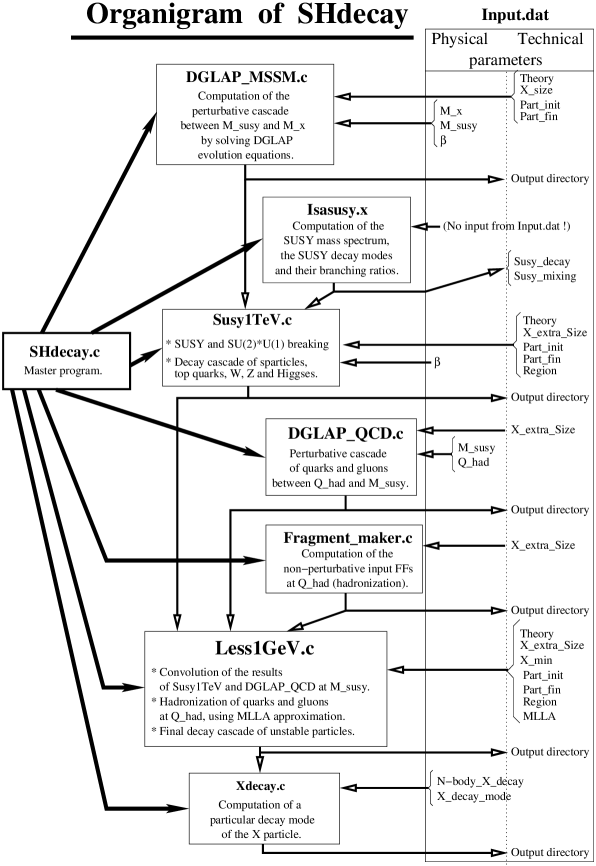
Figure 3: Organigram of SHdecay with the interdependence between the different programs and the needed input parameters for each code.

There are mainly four successive programs treating the different parts of the decay cascade; in order of decreasing virtuality, these are : DGLAP_MSSM, Susy1TeV, DGLAP_QCD, and Less1GeV. Eventually, a last small program called Xdecay can be run to study a particular decay mode of the $X$ particle. I will describe in detail the role of each of these programs, and the parameters of Input.dat they are sensitive to. Fig 3 gives a detailed organigram of the whole code, which shows the interdependences between the different programs and their input parameters.

The whole code SHdecay needs at two different steps the results of other independent codes, namely :

• the SUSY mass spectrum, mixing angles, and decay modes of sparticles (with their branching ratios), all given by ISASUSY (a subset of the Isajet code, written in Fortran 77).

• the non-perturbative input fragmentation functions, computed (once and for all) from the results of [13] through a program called Fragment_maker (which is furnished).

We’ll describe these two secondary procedures in the corresponding subsections.

Of course, the values of all the parameters written in Input.dat should be kept the same for the four programs running successively.

All these programs have been written in C using a few C++ tools. The compiling option of SHdecay is using the g++ compiler of gnu (given by default on Unix and Linux OS).

I first describe all technical parameters before going into the details of each program.

5.1 Technical parameters

• “$X_{\rm Size}$” gives the number of $x$ values used to store the FFs on the interval [$10^{-7}$:$1-10^{-7}$]. Because of 1) the behaviour of the splitting functions at small x, 2) the fact that we are beginning with “delta functions” at large $x$, and 3) the definition of the convolution which is relating the low and large $x$ regions, the two extremities of our interval have to be modelled symmetrically with great accuracy, if we want the integration and (cubic spline) extrapolation procedures to be able to give results at the desired precision of $\sim 10^{-3}$. For this purpose I used a bi-logarithmic scale between [$10^{-7}$:0.5] and [0.5:$1-10^{-7}$], increasing the number of $x$ values towards the two extremities. By default, $X_{\rm Size}=101$, i.e. 50 $x$ values on each side of the central value at $x=0.5$. Note that a smaller value could lead to false results, while increasing $X_{\rm Size}$ is increasing greatly the running time needed by all programs. So I really advise the user not to change this value. Note finally that the smallest $x$ value $10^{-7}$ has been choosen at the limit of the validity of the (leading order) DGLAP equations, before MLLA effects become strong (which happens at $\sqrt{\frac{Q_{had}}{M_{X}}}\sim 10^{-8}$ for $M_{X}\sim 10^{25}$ eV and $Q_{had}\sim 1$ GeV; see [7]). At low $x$, the standard LO DGLAP equations will predict a power law behaviour (option MLLA = 0), but the MLLA approximation (option MLLA = 1), will allow to parameterize some NLO effects like soft gluon emission.

• “$X_{\rm extraSize}$” is a parameter which allows the user to increase homogeneously the overall number of $x$ values on the interval $[10^{-7}:1-10^{-7}]$ after the first program DGLAP_MSSM (which is, once again, the most time consuming part of the complete code). But it is quite useless, the initial value of $X_{\rm Size}$ being large enough for all following programs. By default, $X_{\rm extraSize}$ is simply taken to be equal to $X_{\rm Size}$. Of course, it has to be greater than (or at least equal to !) $X\_{\rm Size}$.

• “Part_init” and “Part_fin” describe the initial and final id’s of an interval of initial particles for which the FFs have to be computed. Note that there are 30 initial particles in the MSSM (see Appendix A for the description of these particles and their id’s), and all the $30\times 30=900$ FFs from any particle to any other will be needed for the computation of the whole cascade. Thus the default values are respectively Part_init $=1$ and Part_fin $=30$, which means that the program will treat successively all the 30 possible initial particles. Nevertheless, the treatment of an initial particle being fully independent of the others, any of the 3 programs DGLAP_MSSM, Susy1TeV and Less1GeV can be cut into pieces to be run independently on different computers; for example, you can let a first computer run the chosen program for particles 1 to 15, and another computer run the same program for particles 16 to 30. These two parameters render this task easy and allow to save a lot of time.
  Caution: Note that each of these three programs has to be run over the whole range of particles before running the following one !

• $X_{\rm min}$ gives the lowest value of the final x interval. As stated above, in the lowest x region ($[X_{\rm min}:10^{-7}]$), you can choose two different extrapolations of the FFs : either extrapolating the power law obtained from the LO DGLAP equations, or using the MLLA approximation for taking color coherence effects into account. This parameter, taken by default to be $X_{min}=10^{-13}$, is only used in the very last part of the computation of the cascade : Less1GeV.
  Caution: of course, $X_{\rm min}$ has to be $\geq 10^{-7}$.

5.2 DGLAP_MSSM

This program treats completely the perturbative cascade above the $M_{\rm SUSY}$ scale. Starting from input FFs at $M_{\rm SUSY}$ for each type of primary particle $P$ ($D_{P}^{P}(x,M_{\rm SUSY})=\delta(1-x)$ and $\forall j\neq P$, $D_{P}^{j}(x,M_{\rm SUSY})=0)$, it gives the FFs of the 30 interaction eigenstates at scale $Q=M_{X}$: $D_{P}^{j}(x,M_{X})$.

By giving the parameters of the “Input.dat” file, the user can choose one of the 4 available theories, namely 1 : MSSM, 2 : SM, 3 : SUSY-QCD, 4 : QCD alone. I point out that this complicated program is certainly not the best one for treating a case as simple as QCD DGLAP equations (or even SUSY-QCD), being unfortunately quite time consuming. This program requires no external input (except Input.dat, of course), and only needs as “physical inputs” the values of $\beta$ and $M_{X}$, described above. The technical parameters $X_{\rm Size}$, “Part_init” and “Part_fin” are used, too. As I already mentioned before, I strongly suggest when possible to run the program on different computers at the same time, using different intervals of initial particles, for saving time.

Finally, the user should specify the corresponding output directory, where the output files will be stored.

Using the structure of the DGLAP evolution equations and $\delta$-functions input FFs at $M_{\rm SUSY}$ (practically implemented as sharp gaussians), this program will compute the full set of FFs from one particle to another between $M_{\rm SUSY}$ and $M_{X}$. For this purpose, I use a Runge-Kutta method with a constant logarithmic step in virtuality for solving the system of DGLAP equations. There must be an entire number of these steps between $M_{SUSY}$ and (any value of) $M_{X}$. That’s why it is only possible to use powers of 10 for these scales. Nevertheless, as I said before, this allows already a good accuracy.

Here we can see the interest of the variable “Nb_output_virtualities” and the corresponding array of virtuality values “Output_virtualities_DGLAP_MSSM” : thanks to the fact that this program is computing the FFs from $M_{SUSY}$ to $M_{X}$ through a given number of Runge-Kutta steps, all intermediate virtualities used by the Runge-Kutta program are available as possible outputs ; it allows to get the FFs at intermediate virtualities, which are equivalent to lower $X$ masses $M_{X}$. As stated above, the step used for Runge-Kutta is a constant logarithmic step, exactly one order of magnitude each. So practically, the user who wants to study a GUT X particle with mass $M_{X}\sim 10^{25}$ eV can get the results for any other (power of 10) $X$ mass ($10^{21}$, $10^{22}$, $10^{23}$ eV,…) between $M_{SUSY}$ and $M_{X}$. The two variables cited above allow to put these partial results in output files that will be usable later on. Note again that only this program will use the array of values for $M_{X}$. The following ones will simply use one of these values, the one given in the parameter $M_{X}$ itself.

The output is presented in $30\times 30=900$ files giving the FFs of any particle into any other with $X_{\rm Size}$ values of x in the first column and the corresponding values of the FF in the second one. These files are called generically “fragment_(M_X)eV_p1.p2” for the FF of particle p1 into particle p2, where (M_X) contains the mass of the $X$ particle at which the FF was computed.

Finally, it is worth noting that the output of this program only depends on very few parameters : the $M_{\rm SUSY}$ scale at which the perturbative cascade is ending, and the SUSY parameter $\tan\beta$. But as stated in [7], these two parameters have very little influence on the final results. Thus I strongly recommend to let run this program only once, for all $X$ masses you want to study, and to carefully keep these partial results for later use, for studying the influence of other parameters appearing in the following programs.

5.3 How to use Isasusy.x

The ISASUSY program, written in fortran 77, is a subset of the whole code called ISAJET. I refer to the user manual of ISASUSY[12] for information about how to use this program. But, as mentioned above, I fully implemented a personalised version of this code, which is available through the master program (option 7). For a given set of SUSY parameters specified by the user in SUSY.dat, it computes the complete SUSY spectrum (masses and mixing angles of all the sparticles, stored in the “Mixing.dat” file), and the allowed decay modes with the corresponding branching ratios (stored in “Decay.dat”). Both files will be stored in the Isasusy directory of SHdecay, and their names have to be given in the “SUSY.dat” input file.

Of course, you can get these files from any other available code providing the same information as ISASUSY, as long as you adapt the output format of this code in order to get the one required by SHdecay (see the model files provided in the Isasusy directory for information about the required format). The furnished version of Isasusy is the one included in Isajet 7.51. If you want to use an updated version of Isasusy, you probably just need to replace the two files called “aldata.f” and “libisajet.a” in the Isasusy repertory of SHdecay (but hopefully not ssrun.f and the Makefile, which I have adapted).Yet, I obviously cannot ensure that this operation will work…

5.4 Susy1TeV

This program takes the results of DGLAP_MSSM given at the (unique) $M_{X}$ value specified in Input.dat and deals with the breaking of SUSY and $SU(2)\otimes U(1)$, the supersymmetric decay cascade and the decays of the top quarks, the Higgs, $W$ and $Z$ bosons. The muons and taus existing at this step are decayed too. I considered only 2- and 3-body decays for which I computed the relevant phase space, using the branching ratios and the mass spectrum given by ISASUSY. For any detail on these procedures, I refer to [7].

The input directory has to be the one where the outputs of DGLAP_MSSM have been stored (the user doesn’t have to specify it). On the other hand, the output directory can be different, in order to distinguish between different parameters. For example, the mass of the $X$ particle, which is especially specified in the names of the output files of DGLAP_MSSM (as being the final virtuality of the perturbative cascade) is no more specified in the outputs of Susy1TeV ; thus it can be usefull to define different output directories for different $X$ masses. Moreover, the large number of output files is easier to handle when stored in different directories.

The program will need the two output files given by Isasusy.x (or any other program, see above); the two files have to be located in the directory “Isasusy”, and their names have to be given in the two corresponding parameters of SUSY.dat : “Decay” and “Mixing”. Here the parameter “Region” also becomes useful. If necessary, the extension of the $x$ array to “$X_{\rm extraSize}$” values instead of “$X_{\rm Size}$” will occur in this program, too.

The output files contain the FFs of the 30 initial particles (interaction eigenstates) into the remaining SM mass eigenstates after the decays, namely the quarks u, d, s, c, b and gluons, the electrons, neutrinos and the LSP. All of them will have a suffix “_1TeV” to distinguish them from the outputs of other programs and a “region”-suffix, e.g. labelling the set of SUSY parameters you used during the run.

5.5 DGLAP_QCD

This program is a simplified copy of DGLAP_MSSM. It computes the pure QCD perturbative partonic cascade for quarks and gluons (so only 6 particles) for a virtuality decreasing from $M_{\rm SUSY}$ to $Q_{\rm had}={\rm max}(m_{\rm quark},1$ GeV). This program is not using any previous result from other ones, and only depends on $M_{\rm SUSY}$ and $Q_{\rm had}$, which are not very sensitive parameters, as stated above. I thus recommend to define their values once and for all (say, keep the default values $M_{\rm SUSY}=1$ TeV and $Q_{\rm had}=1$ GeV), and to run DGLAP_QCD only once. This possiblity of sparing running time is the reason why the necessary convolution between the results of this program and the FFs given by the previous one (Susy1TeV) was implemented in Less1GeV, in order to keep DGLAP_QCD fully independent.

The $6\times 6=36$ output files, called generically “fragment_p1.p2” - where p1 and p2 are initial and final partons {u,d,s,c,b,g} - will be stored in the corresponding directory given in Input.dat. I recommend to use a dedicated directory, for the reason stated above : these results are almost parameter independent and can be used for different runs of Susy1TeV and Less1GeV.

5.6 Fragment_maker

This program is certainly the weakest part of our treatment, because of the lack of knowledge concerning the non-perturbative FFs at very low $x$. I used the results of [13] for this purpose, which are based on LEP data. Unfortunately they are only valid for $x\geq 0.1$. The reason is that at LEP energies, it is necessary to consider mass effects at small $x$, which can be described by the so-called “MLLA plateau”. Such effects can be taken into account during the computation of the hadronization itself, in Less1GeV. In Fragment_maker, just keep the FFs given in [13] up to $x=0.1$ and extrapolate them at small $x$, by requiring continuity and the overall conservation of energy.

We finally obtain a set of input functions for light quarks (including the $b$) and for gluons which conserve energy and agree with known data.

This program is fully independent of the others, and is just used to “prepare” the non-perturbative input FFs at low energy needed in Less1GeV. It doesn’t depend on any parameter, and can be run once and for all. Once again, I recommend to use a dedicated directory for storing the output Files of this program ; the default value is a directory called “Fragment”.

5.7 Less1GeV

This program first computes the convolution between the results of Susy1TeV (describing the evolution of the FFs between $M_{X}$ and $M_{\rm SUSY}$ after SUSY, top, $W$, $Z$ and Higgs decays) and the ones of DGLAP_QCD (describing the further evolution of the partonic part of these FFs between $M_{\rm SUSY}$ and $Q_{\rm had}$). It further deals with the hadronization of quarks and gluons, using external input FFs (The results of the Fragment_maker program described above) which have to be convoluted with the previous results. It finally deals with the decays of the last unstable particles. The 2- and 3-body decays are treated exactly as in Susy1TeV.

The results are once more given in terms of FFs of any initial (interaction eigenstate) particle (between the 30 available in the MSSM, see Appendix A) into the final (physical) stable ones, namely the protons, electrons, photons, three species of neutrinos, and LSPs. To simplify the storing and further use of these (final) results, I grouped all the results corresponding to one initial particle in one file generically called “fragment_p1.all_Region”, where p1 is the initial particle and Region the suffix labelling the set of SUSY parameters. Each file contains seven FFs : the first column gives the values of $x$ (from $1-10^{-7}$ to $X_{\rm min}$, in decreasing order), and the next columns give successively the FFs of p1 into protons, photons, LSPs, electrons, $\nu_{e}$, $\nu_{\mu}$, $\nu_{\tau}$.

5.8 Xdecay

This last program allows to study a special decay mode of the X particle, by computing a last convolution between the results obtained in Less1GeV and the phase space of the given decay mode. The number of decay products and their nature (through the associated id, see Appendix A) have to be specified in Input.dat.

If a decay mode for the $X$ particle has been specified in the two parameters “N-body_X_decay” and “X_decay_mode” (respectively the number $N$ of products and the id’s associated to each product - see Appendix A), a last convolution with the $N$-body decay energy spectrum will be computed and the results will be directly given in terms of the FFs of the $X$ particle into the stable final ones. The $N$-body energy spectrum I used is the one given in [10]. If $\rho_{N}(z)$ is the probability density of obtaining a decay product of energy $E$ carrying the energy fraction $x=2E/M_{X}$ of the decaying particle, we have :

$$\rho_{2}(x)=\delta(1-x)\,,$$

$$\rho_{N}(x)=(N-1)(N-2)x(1-x)^{N-3}\,,N\geqslant 3\,.$$

This program has been separated from Less1GeV to allow the user to obtain very quickly any decay mode he wants to study. The final result is stored in the same directory as the results of Less1GeV. It is generically called “frag_X_a_b_c.all_G” and has the same format as the one described above for the results of Less1GeV.

6 Conclusion

This article describes in some detail how to use the code SHdecay, which has been designed for computing the most general decay spectra of any super-heavy particle in the framework of the MSSM. I hope that it will be of some use for other researchers. The code is available on the web site of our group, under the address :”www1.physik.tu-muenchen.de/ barbot/”, and I will be pleased to answer any question you have about it. Of course, any remark or suggestion is welcome, too.

Appendix A: Description of the compound particles used in SHdecay

Here I describe the 30 interaction eigenstates (or “compound particles”) of the MSSM which have been used as possible decay products for the $X$ particle. As the decay is occuring well above the breaking scales of SUSY and $SU(2)\otimes U(1)$, one has to allow a decay into supersymmetric particles as well as SM particles, and to distinguish between the helicities (Left or Right) of the Dirac fermions; yet, well above the breaking scales of SUSY and $SU(2)\otimes U(1)$, it is assumed that one doesn’t need to distinguish between the components of a given SU(2) multiplet, in particular between the “up” and “down” components of the SU(2) doublets. Moreover, up to the Yukawa couplings which become relevant only for the third generation of fermions, no difference is made between the generations, all particles being massless above the $SU(2)\otimes U(1)$ breaking scale. If we consider a perfect CP symmetry, one doesn’t need to distinguish between particles and antiparticles, either. In summary, for example, the fields ($u_{L}$, $d_{L}$), ($c_{L}$, $s_{L}$), ($\bar{u}_{L}$, $\bar{d}_{L}$), and ($\bar{c}_{L}$, $\bar{s}_{L}$) all obey exactly the same DGLAP evolution equation and thus can be considered as a single “particle” which is taken to be an average over all these fields. This “coumpound particle” is called $q_{L}$ in our nomenclature and has id 1. I give in table 1 all fermionic compound particles I used, together with the associated superparticles, and their respective id’s.

The same occurs for bosons and bosinos, where we only have to consider the unbroken fields $B$, $W$, $g$ (for gluons), the two SU(2) Higgs doublets of the MSSM $H_{1}$ (coupled to leptons and down-type quarks of the third generation) and $H_{2}$ (coupled to the up-type quarks of the third generation), and their superpartners. The well known particles and antiparticles at lower energies are mixtures of the components of these interaction eigenstates. I give the corresponding id’s in table 2.

Test Run Input and Output

I give here a test run for a very simple case that can be computed in a few hours: the “Input_ex.dat” file and the final “Output_ex.dat” file given by SHdecay for a $X$ particle with $M\_X=10^{10}$ GeV in the pure QCD case (Theory = 4).

Input_ex.dat:

Theory: 4

MLLA: 1

Nb_output_virtualities: 1

Output_virtualities_DGLAP_MSSM(GeV): 1.e10

M_x(GeV): 1.e10

N-body_X_decay: 2

X_decay_mode: 1 1

M_Susy: 1.e3

Q_had: 1.

X_Size: 101

X_extra_Size: 101

Part_init: 1

Part_fin: 30

X_min: 1.e-13

Region: G

Output_file: ./QCD/Output_ex.dat

Output_directory(DGLAP_MSSM.c): QCD

Output_directory(Susy1TeV.c): QCD

Output_directory(DGLAP_QCD.c): QCD/DGLAP_QCD

Output_directory(Fragment_maker.c): Fragment

Output_directory(Less1GeV.c): QCD

Output_ex.dat:

********************** Input Parameters **********************

THEORY = 4 (1 for MSSM, 2 for SM, 3 for Susy-QCD, 4 for QCD alone)
MLLA = 1 (1 for MLLA approximation, 0 for power laws at small x)
Virtualities at which DGLAP_MSSM is storing results in output files : Mx[0] = 1e+10 GeV
Mass of the X particle (it must be one of the virtualities at which results have been stored !): Mx = 1e+10 GeV
Number of decay products of the X particle : 2
Decay mode of the X particle :1 1
Susy scale : 1000 GeV
Hadronization scale : 1 GeV
Beta = 1.29985

X_Size (in DGLAP_MSSM): 101
X_extra_Size (everywhere else) : 101
Xmin : 1e-13
Computation from part 1 to part 30
Region : G (For example, G for Gaugino-like LSP, H for Higgsino-like LSP)

DGLAP_MSSM output directory = QCD
Susy1TeV output directory = QCD
DGLAP_QCD output directory = QCD/DGLAP_QCD
Fragment_maker output directory = Fragment
Final output directory = QCD

********************** Susy1TeV ***************************

Initial Particle 1 = uL
—————————–

uL $->$ quarks + gluons = 0.998024
uL $->$ gamma = 0
uL $->$ LSP = 0
uL $->$ e = 0.000174832
uL $->$ Nu_e = 0.000174743
uL $->$ nu_mu = 0.000174463
uL $->$ nu_tau = 0.00016671
uL $->$ Total = 0.998715

[…]

*********************** DGLAP_QCD ************************

[…]

PARTON = 5
——————

At final t:

Partial energy from 0 into 5 = 0.0502139
Partial energy from 1 into 5 = 0.00935672
Partial energy from 2 into 5 = 0.00935672
Partial energy from 3 into 5 = 0.00935672
Partial energy from 4 into 5 = 0.00935672
Partial energy from 5 into 5 = 0.69335

Integrated energy from 0 = 0.997878
Integrated energy from 1 = 0.998345
Integrated energy from 2 = 0.998345
Integrated energy from 3 = 0.998345
Integrated energy from 4 = 0.998339
Integrated energy from 5 = 0.998346

********************** Fragment_maker **********************

Total energy fractions contained in the extrapolated FFs (including the hadronic Peterson contribution for heavy quarks c and b) :
(should be very close to 1. !)

Energy fraction [u] = 0.997544
Energy fraction [d] = 0.997544
Energy fraction [s] = 0.996595
Energy fraction [c] = 1.07197
Energy fraction [b] = 1.032
Energy fraction [g] = 1.00657

********************** Less1GeV **************************

Initial Particle 1 = uL
—————————–

uL $->$ protons = 0.112688
uL $->$ gamma = 0.253301
uL $->$ LSP = 0
uL $->$ e = 0.162863
uL $->$ Nu_e = 0.160729
uL $->$ nu_mu = 0.3005
uL $->$ nu_tau = 0.000698547
uL $->$ Total = 0.990781

[…]

********************** X_decay ***************************

Total fraction of energy carried by decay product 1 = 0.990781

(This result should be close to 1., in order to respect the energy conservation over the whole cascade)

Total fraction of energy carried by decay product 0 = 0.990781

(This result should be close to 1., in order to respect the energy conservation over the whole cascade)

Energy fraction carried by the X particle = 1.98156

(This result should be almost equal to 2, because the mass of the X particle is twice the energy fraction provided to any of its decay products. In this final result, the total energy carried by all FFs is naturally equal to the mass of the initial particle !)

*************************************************************

In order to illustrate the type of results that one can get in the most general case (MSSM framework, Theory = 1), I give in fig. 1 an example of output fragmentation functions obtained with SHdecay for initial $u_{L}$ quark (id. 1 in Appendix A) and $\tilde{u}_{L}$ squark (id. 7 in Appendix A), for one set of SUSY parameters, with low $\tan\beta$ and gaugino–like LSP. I used the default values of the furnished files Input.dat and SUSY.dat (i.e. a ratio of Higgs vevs $\tan\beta=3.6$, a gluino and scalar mass scale $M_{\rm SUSY}\sim 1000$ GeV, a supersymmetric Higgs mass parameter $\mu=500$ GeV, a CP–odd Higgs boson mass $m_{A}=1000$ GeV and trilinear soft breaking parameter $A_{t}=1$ TeV). As usual, I plot $x^{3}\cdot D_{I}^{P}(x,M_{X})$. I take $M_{X}=10^{16}$ GeV, as appropriate for a GUT interpretation of the $X$ particle.

Figure 1: Fragmentation functions of a first or second generation $SU(2)$ doublet quark (top) and a squark (bottom) into stable particles.

compound particle	id
$q_{L}=\frac{1}{4}\left[\left(\frac{u_{L}}{d_{L}}\right)+\left(\frac{c_{L}}{s_{L}}\right)+\left(\frac{\bar{u}_{L}}{\bar{d}_{L}}\right)+\left(\frac{\bar{s}_{L}}{\bar{c}_{L}}\right)\right]$	1
$q_{R}=\frac{1}{4}\left[u_{R}+c_{R}+\bar{u}_{R}+\bar{c}_{R}\right]$	2
$d_{R}=\frac{1}{4}\left[d_{R}+s_{R}+\bar{d}_{R}+\bar{s}_{R}\right]$	3
$t_{L}=\frac{1}{2}\left[\left(\frac{t_{L}}{b_{L}}\right)+\left(\frac{\bar{t}_{L}}{\bar{b}_{L}}\right)\right]$	4
$t_{R}=\frac{1}{2}(t_{R}+\bar{t}_{R})$	5
$b_{R}=\frac{1}{2}(b_{R}+\bar{b}_{R})$	6
$\tilde{q}_{L}=\frac{1}{4}\left[\left(\frac{\tilde{u}_{L}}{\tilde{d}_{L}}\right)+\left(\frac{\tilde{c}_{L}}{\tilde{s}_{L}}\right)+\left(\frac{\tilde{\bar{u}}_{L}}{\tilde{\bar{d}}_{L}}\right)+\left(\frac{\tilde{\bar{s}}_{L}}{\tilde{\bar{c}}_{L}}\right)\right]$	7
$u_{R}=\frac{1}{4}\left[\tilde{u}_{R}+\tilde{c}_{R}+\tilde{\bar{u}}_{R}+\tilde{\bar{c}}_{R}\right]$	8
$d_{R}=\frac{1}{4}\left[\tilde{d}_{R}+\tilde{s}_{R}+\tilde{\bar{d}}_{R}+\tilde{\bar{s}}_{R}\right]$	9
$t_{L}=\frac{1}{2}\left[\left(\frac{\tilde{t}_{L}}{\tilde{b}_{L}}\right)+\left(\frac{\tilde{\bar{t}}_{L}}{\tilde{\bar{b}}_{L}}\right)\right]$	10
$t_{R}=\frac{1}{2}(\tilde{t}_{R}+\tilde{\bar{t}}_{R})$	11
$b_{R}=\frac{1}{2}(\tilde{b}_{R}+\tilde{\bar{b}}_{R})$	12
$l_{L}=\frac{1}{4}\left[\left(\frac{e_{L}}{\nu_{e}}\right)+\left(\frac{\mu_{L}}{\nu_{\mu}}\right)+\left(\frac{\bar{e}_{L}}{\bar{\nu}_{e}}\right)+\left(\frac{\bar{\mu}_{L}}{\bar{\nu}_{\mu}}\right)\right]$	13
$l_{R}=\frac{1}{4}\left[e_{R}+\mu_{R}+\bar{e}_{R}+\bar{\mu}_{R}\right]$	14
$\tau_{L}=\frac{1}{2}\left[\left(\frac{\tau_{L}}{\nu_{\tau}}\right)+\left(\frac{\bar{\tau}_{L}}{\bar{\nu}_{\tau}}\right)\right]$	15
$\tau_{R}=\frac{1}{2}(\tau_{R}+\bar{\tau}_{R})$	16
$\tilde{l}_{L}=\frac{1}{4}\left[\left(\frac{\tilde{e}_{L}}{\tilde{\nu}_{e}}\right)+\left(\frac{\tilde{\mu}_{L}}{\tilde{\nu}_{\mu}}\right)+\left(\frac{\tilde{\bar{e}}_{L}}{\tilde{\bar{\nu}}_{e}}\right)+\left(\frac{\tilde{\bar{\mu}}_{L}}{\tilde{\bar{\nu}}_{\mu}}\right)\right]$	17
$l_{R}=\frac{1}{4}\left[\tilde{e}_{R}+\tilde{\mu}_{R}+\tilde{\bar{e}}_{R}+\tilde{\bar{\mu}}_{R}\right]$	18
$\tau_{L}=\frac{1}{2}\left[\left(\frac{\tilde{\tau}_{L}}{\tilde{\nu}_{\tau}}\right)+\left(\frac{\tilde{\bar{\tau}}_{L}}{\tilde{\bar{\nu}}_{\tau}}\right)\right]$	19
$\tau_{R}=\frac{1}{2}(\tilde{\tau}_{R}+\tilde{\bar{\tau}}_{R})$	20

Table 1: Definition and id’s of the compound SM fermions and their superpartners in SHdecay.

compound particle	id
$W=\frac{1}{3}(W_{1}+W_{2}+W_{3})$	21
$B$	22
$g$	23
$H_{1}=\frac{1}{2}(H_{1}^{1}+H_{1}^{2})$	24
$H_{2}=\frac{1}{2}(H_{2}^{1}+H_{2}^{2})$	25
$\tilde{W}=\frac{1}{3}(\tilde{W}_{1}+\tilde{W}_{2}+\tilde{W}_{3})$	26
$\tilde{B}$	27
$\tilde{g}$	28
$\tilde{H}_{1}=\frac{1}{2}(\tilde{H}_{1}^{1}+\tilde{H}_{1}^{2})$	29
$\tilde{H}_{2}=\frac{1}{2}(\tilde{H}_{2}^{1}+\tilde{H}_{2}^{2})$	30

Table 2: Definition and id’s of the compound bosonic SM particles and their superpartners in SHdecay.

Figure 2: Schematic MSSM cascade for an initial squark with a virtuality $Q\simeq M_{X}$. The full circles indicate decays of massive particles, in distinction to fragmentation vertices. The two vertical dashed lines separate different epochs of the evolution of the cascade: at virtuality $Q>M_{\rm SUSY}$, all MSSM particles can be produced in fragmentation processes. Particles with mass of order $M_{\rm SUSY}$ decay at the first vertical line. For $M_{\rm SUSY}>Q>Q_{\rm had}$ light QCD degrees of freedom still contribute to the perturbative evolution of the cascade. At the second vertical line, all partons hadronize, and unstable hadrons and leptons decay. See the text for further details.

References

- [1] S. P. Martin, In Kane, G.L. (ed.): Perspectives on supersymmetry, 1-98, hep-ph/9709356.
- [2] D.J.H. Chung, E.W. Kolb and A. Riotto, Phys. Rev. D60 (1999) 0603504, hep-ph/9809453; D.J. Chung, P. Crotty, E.W. Kolb and A. Riotto, Phys. Rev. D64 (2001) 043503, hep-ph/0104100; R. Allahverdi and M. Drees, Phys. Rev. Lett. 89 (2002) 091302, hep-ph/0203118, and Phys. Rev. D66 (2002) 063513, hep-ph/0205246.
- [3] P. Bhattacharjee and G. Sigl, Phys. Rept. 327 (2000) 109, astro-ph/9811011; L. Anchordoqui, T. Paul, S. Reucroft and J. Swain, Int. J. Mod. Phys. A 18 (2003) 2229 hep-ph/0206072.
- [4] M. A. Lawrence, R. J. O. Reid, and A. A. Watson, J. Phys. G17 (1991) 733; D. J. Bird et al., Astrophys. J. 441 (1995) 144; HiRes-MIA collab., T. Abu-Zayyad et al., Astrophys. J. 557 (2001) 686, astro-ph/0010652; AGASA collab., N. Hayashida et al., Astrophys. J. 522 (1999) 225, astro-ph/0008102.
- [5] G. Altarelli and G. Parisi, Nucl. Phys. B126 (1977) 298.
- [6] C. Barbot and M. Drees, Phys. Lett. B533 (2002) 107, hep-ph/0202072.
- [7] C. Barbot and M. Drees, hep-ph/0211406, accepted for publication in Astroparticle Physics.
- [8] V. Berezinsky and M. Kachelriess, Phys. Rev. D63 (2001) 034007, hep-ph/0009053.
- [9] C. Coriano and A. E. Faraggi, Phys. Rev. D65 (2002) 075001, hep-ph/0106326.
- [10] S. Sarkar and R. Toldra, Nucl. Phys. B621 (2002) 495, hep-ph/0108098.
- [11] A. Ibarra and R. Toldra, JHEP 0206, (2002) 006 hep-ph/0202111.
- [12] H. Baer, F. E. Paige, S. D. Protopopescu, and X. Tata, hep-ph/9305342.
- [13] B. A. Kniehl, G. Kramer, and B. Potter, Nucl. Phys. B582 (2000) 514–536, hep-ph/0010289.
- [14] E. Reya Phys. Rept. 69 (1981) 195.
- [15] C. Barbot, M. Drees, F. Halzen, and D. Hooper, Phys. Lett. B555 (2003) 22, hep-ph/0205230.
- [16] C. Barbot, M. Drees, F. Halzen, and D. Hooper, hep-ph/0207133, accepted for publication in Phys. Lett. B..
- [17] S. K. Jones and C. H. Llewellyn Smith, Nucl. Phys. B217 (1983) 145.
- [18] Y. L. Dokshitzer, V. A. Khoze, A. H. Mueller, and S. I. Troian,, Basics of perturbative QCD. Gif-sur-Yvette, France: Ed. Frontieres (1991) 274 p. (Basics of).
- [19] P. Gondolo, G. Gelmini and S. Sarkar, Nucl. Phys. B392 (1993) 111, hep-ph/9209236; F. Halzen and D. Hooper, Rept. Prog. Phys. 65 (2002) 1025, astro-ph/0204527.
- [20] Y.I. Azimov, Y.L. Dokshitzer, V.A. Khoze and S.I. Troian, Phys. Lett. B165 (1985) 147, and Z. Phys. C27 (1985) 65.
- [21] C. P. Fong and B. R. Webber, Phys. Lett. B229 (1989) 289.
-
[22]
V. Berezinsky and M. Kachelriess, Phys. Lett. B434 (1998) 61,
t hep-ph/9803500.