Charmless hadronic decays $B\to VV$ in the Topcolor-assisted Technicolor model

Abstract

Based on the effective Hamiltonian with the generalized factorization approach, we calculate the branching ratios and CP asymmetries of $B\to VV$ decays in the Topcolor-assisted Technicolor (TC2) model. Within the considered parameter space we find that: (a) for the penguin-dominated $B\to K^{*+}\phi$ and $K^{*0}\phi$ decays, the new physics enhancements to the branching ratios are around $40\%$; (b) the measured branching ratios of $B\to K^{*+}\phi$ and $K^{*0}\phi$ decays prefer the range of $3\lesssim N_{c}^{eff}\lesssim 5$; (c) the SM and TC2 model predictions for the branching ratio ${\cal B}(B^{+}\to\rho^{+}\rho^{0})$ are only about half of the Belle’s measurement; and (d) for most $B\to VV$ decays, the new physics corrections on their CP asymmetries are generally small or moderate in magnitude and insensitive to the variation of $m_{\tilde{\pi}}$ and $N_{c}^{eff}$.

I Introduction

As is well-known, one of the main goals of B experiments is to find the evidence or signals of new physics beyond the standard model (SM). Precision measurements of B meson system can provide an insight into very high energy scales via the indirect loop effects of new physics[1, 2], and offer a complementary probe to the searches for new physics in future collider runs at the Tevatron, and the LHC, and the future linear $e^{+}e^{-}$ colliders.

Theoretically, the low energy effective Hamiltonian[3] is our basic tool to study the B meson decays. The short-distance QCD corrected Lagrangian at next-to-leading order (NLO) is available now, but we still do not know how to calculate hadronic matrix elements from first principles. The generalized factorization (GF) ansatz [4, 5, 6] is widely used in literature [5, 7, 8, 9], and the resulted predictions are basically consistent with the experimental measurements. But we also know that non-factorizable contribution really exists and can not be neglected numerically for many hadronic B decay channels. Two new approaches, called as the QCD factorization [10] and the perturbative QCD approach[11], appeared recently and played an important role in reducing the uncertainties of the corresponding theoretical predictions[10, 11, 12, 13].

During the past three decades, many new physics models beyond the SM have been constructed. The most popular one is certainly the minimal supersymmetric standard model (MSSM), another alternative to break the electroweak symmetry is the Technicolor mechanism[14]. The Topcolor-assisted Technicolor (TC2) model[15] is a viable model and consistent with current experimental data[16, 17, 18]. In paper[17] we calculated the new electroweak penguin contributions to the rare K decays in the TC2 model. In a recent paper[18], we presented our systematic calculation of branching ratios and CP-violating asymmetries for two-body charmless hadronic decays $B\to PP$, $PV$ (the light pseudo-scalar (P) and/or vector(V) mesons ) in the framework of TC2 model [15]. It is natural to extend our study to the cases of $B\to VV$ decays.

$B\to VV$ decays have been studied frequently in the SM and new physics models, for example, in Refs.[5, 8, 19, 20, 21]. Three decay modes, $B\to K^{*+}\phi,K^{*0}\phi$ and $\rho^{+}\rho^{0}$ decays, have been measured recently by CLEO, BaBar and Belle Collaborations [22, 23, 24, 25, 26]. In this paper, we will concentrate on the new physics effects on nineteen charmless $B\to VV$ decays.

This paper is organized as follows. In Sec. 2, we give a brief introduction for the TC2 model and examine the constraints on the parameter space of the TC2 model. In Sec. 3, based on previous analytical calculations of new penguin diagrams, we find the effective Wilson coefficients $C_{i}^{eff}$ and effective numbers $a_{i}$ with the inclusion of new physics contributions. In Sec. 4 and 5, we calculate and show the numerical results of branching ratios and CP-violating asymmetries for all nineteen $B\to VV$ decay modes, respectively. We focus on those measured decay modes. The conclusions are included in the final section.

II Basics of the TC2 model

Apart from some differences in group structure and/or particle contents, all TC2 models have the similar common features. In this paper we chose the well-motivated and most frequently studied TC2 model proposed by Hill [15] as the typical TC2 model to calculate the new physics contributions to the B decays in question.

In the TC2 model, there exist top-pions $\tilde{\pi}^{\pm}$ and $\tilde{\pi}^{0}$, charged b-pions $\tilde{H}^{\pm}$ and neutral b-pions $(\tilde{H}^{0},\tilde{A}^{0})$, and the techni-pions $\pi_{1}^{\pm}$ and $\pi_{8}^{\pm}$. The couplings of top-pions to t- and b-quark can be written as [15]:

$$\frac{m_{t}^{*}}{F_{\tilde{\pi}}}\left[i\bar{t}t\tilde{\pi}^{0}+i\overline{t}_{R}b_{L}\tilde{\pi}^{+}+\frac{m_{b}^{*}}{m_{t}^{*}}\overline{t}_{L}b_{R}\tilde{\pi}^{+}+h.c.\right]$$ (1)

here, $m_{t}^{*}=(1-\epsilon)m_{t}$ and $m_{b}^{*}\approx 1GeV$ denote the masses of top and bottom quarks generated by topcolor interactions. At low energy, potentially large FCNCs arise when the quark fields are rotated from their weak eigenbasis to their mass eigenbasis, realized by the matrices $U_{L,R}$ and $D_{L,R}$:

$$b_{L}\to D_{L}^{bd}d_{L}+D_{L}^{bs}s_{L}+D_{L}^{bb}b_{L},$$ (2)

$$b_{R}\to D_{R}^{bd}d_{R}+D_{R}^{bs}s_{R}+D_{R}^{bb}b_{R},$$ (3)

the FCNC interactions will be induced

$$\frac{m_{t}^{*}}{F_{\tilde{\pi}}}\left[i\tilde{\pi}^{+}(D_{L}^{bs}\bar{t}_{R}s_{L}+D_{L}^{bd}\bar{t}_{R}d_{L})+i\tilde{H}^{+}(D_{R}^{bs}\bar{t}_{L}s_{R}+D_{R}^{bd}\bar{t}_{L}d_{R})+h.c.\right]$$ (4)

For the mixing matrices in the TC2 model, authors usually use the ”square-root ansatz”: to take the square root of the standard model CKM matrix ($V_{CKM}=U_{L}^{+}D_{L}$) as an indication of the size of realistic mixings. It should be denoted that the square root ansatz must be modified because of the strong constraints from the data of $B^{0}-\overline{B^{0}}$ mixing [16]. By taking into account the experimental constraints, we naturally set $D_{L}^{bd}=V_{td}/2$, and $D_{L}^{bs}=V_{ts}/2$ and $D_{R}=0$ in the numerical calculations[18]. Under this assumption, only the charged top-pions $\tilde{\pi}^{\pm}$ and the charged technipions $\pi_{1}^{\pm}$ and $\pi_{8}^{\pm}$ contribute to the inclusive charmless decays $b\to s\bar{q}q,\;d\bar{q}q$ with $q\in\{u,d,s\}$ through the strong and electroweak penguin diagrams, and the top-pion $\tilde{\pi}^{\pm}$ dominates the new physics contributions within the reasonable parameter space.

Based on previous studies[18], the data of $B\to X_{s}\gamma$ decay result in strong constraint on TC2 model, specifically on the mass of top-pions:

$$140GeV\lesssim m_{\tilde{\pi}}\lesssim 220GeV,$$ (5)

for $\mu=m_{b}/2-2m_{b}$, $\epsilon=0.05\pm 0.03$.

In the numerical calculations, we use the same input parameters of the TC2 model as being used in Ref.[18]:

$$F_{\tilde{\pi}} = 50GeV,\;F_{\pi}=120GeV,\;\epsilon=0.05,$$ (6)

$$m_{\pi_{1}} = 100GeV,\;m_{\pi_{8}}=200GeV,\;m_{\tilde{\pi}}=200^{+20}_{-50}GeV,$$ (7)

where $F_{\pi}$ and $F_{\tilde{\pi}}$ are the decay constants for technipions and top-pions, respectively.

III Effective Wilson coefficients

The standard theoretical frame to calculate the inclusive three-body decays $b\to s\bar{q}q$ is based on the effective Hamiltonian [5],

$${\cal H}_{eff}(\Delta B=1)=\frac{G_{F}}{\sqrt{2}}\left\{\sum_{j=1}^{2}C_{j}\left(V_{ub}V_{us}^{*}Q_{j}^{u}+V_{cb}V_{cs}^{*}Q_{j}^{c}\right)-V_{tb}V_{ts}^{*}\left[\sum_{j=3}^{10}C_{j}Q_{j}+C_{g}Q_{g}\right]\right\},$$ (8)

where the operator $Q_{1}$ and $Q_{2}$ are current-current operators, $Q_{3}-Q_{6}$ are QCD penguin operators induced by gluonic penguin diagrams, and the operators $Q_{7}-Q_{10}$ are generated by electroweak penguins and box diagrams. The operator $Q_{g}$ is the chromo-magnetic dipole operator generated from the magnetic gluon penguin. Following Ref.[5], we also neglect the effects of the electromagnetic penguin operator $Q_{7\gamma}$, and do not consider the effect of the weak annihilation and exchange diagrams.

The new strong and electroweak penguin diagrams can be obtained from the corresponding penguin diagrams in the SM by replacing the internal $W^{\pm}$ lines with the unit-charged scalar ($\pi_{1}^{\pm},\pi_{8}^{\pm}$ and $\tilde{\pi}^{\pm}$ ) lines, as shown in Fig.1 of Ref.[18]. The new physics will manifest itself by modifying the corresponding Inami-Lim functions $C_{0}(x),D_{0}(x),E_{0}(x)$ and $E^{\prime}_{0}(x)$ which determine the coefficients $C_{3}(M_{W}),\ldots,C_{10}(M_{W})$ and $C_{g}(M_{W})$. These modifications, in turn, will change for example the standard model predictions for the branching ratios and CP-violating asymmetries for $B\to VV$ decays. For the sake of simplicity, we here use the results as given in Ref.[18] directly. For more details of the analytical evaluations of new Feynman diagrams, one can see Ref.[18].

By using QCD renormalization group equations[3], it is straightforward to run Wilson coefficients $C_{i}(M_{W})$ from the scale $\mu=O(M_{W})$ down to the lower scale $\mu=O(m_{b})$. Working consistently to the NLO precision, the Wilson coefficients $C_{i}$ for $i=1,\ldots,10$ are needed in NLO precision, while it is sufficient to use the leading logarithmic value for $C_{g}$. The NLO Wilson coefficients are renormalization scale and scheme dependent, but such dependence will be cancelled by the corresponding dependence in the matrix elements of the operators in ${\cal H}_{eff}$. In the NDR scheme and for $SU(3)_{C}$, the effective Wilson coefficients $C_{i}^{eff}$ can be written as [5, 9],

$$C_{i}^{eff} = \left[1+\frac{\alpha_{s}}{4\pi}\,\left(\gamma^{(0)T}\log\frac{m_{b}}{\mu}+\hat{r}^{T}\right)\right]_{ij}\,C_{j}$$ (10)

$$+\frac{\alpha_{s}}{24\pi}\,A_{i}\left(C_{t}+C_{p}+C_{g}\right)+\frac{\alpha_{em}}{8\pi}\,B_{i}C_{e}~{},$$

where $A_{i}=(0,0,-1,3,-1,3,0,0,0,0)^{T}$, $B_{i}=(0,0,0,0,0,0,1,0,1,0)^{T}$, the matrices $\hat{r}_{V}$ and $\gamma_{V}$ contain the process-independent contributions from the vertex diagrams. The anomalous dimension matrix $\gamma_{V}$ has been given explicitly, for example, in Refs.[9, 18]. The explicit expressions of functions $C_{t}$, $C_{p}$, and $C_{g}$ in Eq.(10) can be found in previous paper [18]. Following Refs.[5, 9], we use $k^{2}=m_{b}^{2}/2\pm 2$ in the numerical calculation. In fact, branching ratios considered here are not sensitive to the value of $k^{2}$ within the range of $k^{2}=m_{b}^{2}/2\pm 2$, but the CP-violating asymmetries are sensitive to the variation of $k^{2}$.

IV Branching ratios of $B\to VV$ decays

With the factorization ansatz [4, 5, 9], the decay amplitude $<XY|H_{eff}|B>$ can be factorized into a sum of products of two current matrix elements $<X|J_{1}^{\mu}|0>$ and $<Y|J_{2\mu}|B>$ ( or $<Y|J_{1}^{\mu}|0>$ and $<X|J_{2\mu}|B>$). For $B\to VV$ decays, one needs to evaluate the helicity matrix element $H_{\lambda}=<V_{1}(\lambda)V_{2}(\lambda)|H_{eff}|B)>$ with $\lambda=0,\pm 1$. In the B-rest frame, the branching ratio of the decay $B\to V_{1}V_{2}$ is given in terms of $H_{\lambda}$ by

$${\cal B}(B\to V_{1}V_{2}) = \tau_{B}\,\frac{|p|}{8\pi M_{B}^{2}}\left(|H_{0}|^{2}+|H_{+1}|^{2}+|H_{-1}|^{2}\right),$$ (11)

where $\tau(B_{u}^{-})=1.674ps$ and $\tau(B_{d}^{0})=1.542ps$ [27], $|p|$ is the magnitude of momentum of particle $V_{1}$ and $V_{2}$ in the B rest frame

$$|p|=\frac{1}{2M_{B}}\sqrt{[M_{B}^{2}-(M_{1}+M_{2})^{2}][M_{B}^{2}-(M_{1}-M_{2})^{2}]},$$ (12)

where $M_{B}$ and $M_{i}$ ($i=1,2$) are the masses of B meson and $V_{i}$ vector meson. The three independent helicity amplitudes $H_{0}$, $H_{+1}$ and $H_{-1}$ can be expressed by three invariant amplitudes $a,b,c$ defined by the decomposition

$$H_{\lambda} = i\epsilon^{\mu}(\lambda)\eta^{\nu}(\lambda)\left[ag_{\mu\nu}+\frac{b}{M_{1}M_{2}}p_{\mu}p_{\nu}+\frac{ic}{M_{1}M_{2}}\epsilon_{\mu\nu\alpha\beta}p_{1}^{\alpha}p^{\beta}\right],$$ (13)

where $p_{i}$ ($i=1,2$) is the four momentum of $V_{i}$, and $p=p_{1}+p_{2}$ is the four-momentum of B meson, and

$$H_{\pm 1}=a\pm c\sqrt{x^{2}-1},~{}~{}~{}~{}H_{0}=-ax-b\left(x^{2}-1\right),$$ (14)

with

$$x=\frac{M_{B}^{2}-M_{1}^{2}-M_{2}^{2}}{2M_{1}M_{2}}$$ (15)

For individual decay mode, the coefficients $a,b$ and $c$ can be determined by comparing the helicity amplitude $H_{\lambda}=<V_{1}(\lambda)V_{2}(\lambda)|H_{eff}|B)>$ with the expression (13).

In the generalized factorization ansatz [5, 9], the effective Wilson coefficients $C_{i}^{eff}$ will appear in the decay amplitudes in the combinations,

$$a_{2i-1}\equiv C_{2i-1}^{eff}+\frac{{C}_{2i}^{eff}}{N_{c}^{eff}},\ \ a_{2i}\equiv C_{2i}^{eff}+\frac{{C}_{2i-1}^{eff}}{N_{c}^{eff}},\ \ \ (i=1,\ldots,5),$$ (16)

where the effective number of colors $N_{c}^{eff}$ is treated as a free parameter varying in the range of $2\leq N_{c}^{eff}\leq\infty$, in order to model the nonfactorizable contribution to the hadronic matrix elements. We here will not consider the possible effects of final state interaction (FSI) and the contributions from annihilation channels although they may play a significant rule for some $B\to VV$ decays.

In numerical calculations, one usually uses two sets of form factors at the zero momentum transfer from the Baner, Stech and Wirbel (BSW) model [4], as well as the Lattice QCD and Light-cone QCD sum rules (LQQSR), respectively. Since the differences induced by using two different sets of form factors are small when compared with that of the new physics contributions, we here use the BSW form factors only and list them in Appendix. In the following numerical calculations, we use the decay amplitudes as given in Appendix A of Ref.[5] directly without further discussions about the details.

In Table I, we present the numerical results of the branching ratios for the nineteen $B\to VV$ decays in the framework of the SM and TC2 model. The branching ratios are the averages of the branching ratios of $B$ and anti-$B$ decays. The theoretical predictions are made by using the central values of input parameters as given in Appendix, and assuming $m_{\tilde{\pi}}=200$GeV and $N_{c}^{eff}=2,3,\infty$ in the GF approach. The $k^{2}$-dependence of the branching ratios is weak in the range of $k^{2}=m_{b}^{2}/2\pm 2\;GeV^{2}$ and hence the numerical results are given by fixing $k^{2}=m_{b}^{2}/2$.

Following Ref.[5], the nineteen decay channels under study are also classified into five classes as specified in the second column of Table I. The first three kinds of decays are tree-dominated. The amplitudes of the class-IV decays involve one (or more) of the dominant penguin coefficients $a_{4,6,9}$ with constructive interference among them and these decays are generally $N_{c}^{eff}$ stable. The class-V decays, however, are generally not stable against $N_{c}^{eff}$ since the amplitudes of these decays involve large and delicate cancellations due to interference between strong $N_{c}^{eff}$-dependent coefficients $a_{3},a_{5},a_{7}$, and $a_{10}$ and the dominant penguin coefficients $a_{4},a_{6},a_{9}$.

Among the nineteen decay modes, only $B\to K^{*+}\phi$, $K^{*0}\phi$ and $B\to\rho^{+}\rho^{0}$ decays are measured experimentally [22, 23, 24, 25],

$${\cal B}(B^{0}\to K^{*0}\phi) = (9.8\pm 2.2)\times 10^{-6}\ \ {\rm[weighted-average\cite[cite]{[\@@bibref{Number}{prl86-3718,prl87-151801,belle-0113}{}{}]}]},$$ (17)

$${\cal B}(B^{+}\to K^{*+}\phi) = (10.0\pm 3.7)\times 10^{-6}\ \ {\rm[weighted-average\cite[cite]{[\@@bibref{Number}{prl86-3718,prl87-151801}{}{}]}]},$$ (18)

and

$${\cal B}(B\to\rho^{+}\rho^{0}) = (38.5\pm 10.9(stat.)^{+5.9}_{-5.4}(syst.)^{+2.5}_{-7.5}(pol.))\times 10^{-6}\ \ {\rm[Belle\cite[cite]{[\@@bibref{Number}{belle-0255}{}{}]}]},$$ (19)

where the third error is the error associated with the helicity-mix uncretainty[25]. The available upper limits ($90\%$ C.L.) on other decay modes are taken directly from Ref.[27].

For the measured $B\to K^{*0}\phi$ and $K^{*+}\phi$ decays, the theoretical predictions in the SM and TC2 model have a strong dependence on the value of $N_{c}^{eff}$, as illustrated in Figs.1 and 2 where the solid and short-dashed curves show the theoretical predictions in the SM and the TC2 model, respectively. The data clearly prefer the range of $3\lesssim N_{c}^{eff}\lesssim 5$.

For the branching ratio ${\cal B}(B\to\rho^{+}\rho^{0})$, the SM prediction is $(8.7-16.2)\times 10^{-6}$ for $2\leq N_{c}^{eff}\leq\infty$, as illustrated in Fig.3, which is much smaller than the first measurement as reported by Belle Collaboration[25]. The new physics contribution is also negligibly small: less than $1\%$ with respect to the SM prediction. Of cause, the Belle’s measurement still has a large uncertainty and need to be confirmed by further measurements.

V CP asymmetries in $B\to VV$ decays

In TC2 model, no new weak phase has been introduced through the interactions involving new particles and hence the mechanism of CP violation in TC2 model is the same as in the SM. But the CP-violating asymmetries ${\cal A}_{CP}$ may be changed by the inclusion of new physics contributions through the interference between the ordinary tree/penguin amplitudes in the SM and the new strong and electroweak penguin amplitudes in TC2 model.

For charged B decays the direct CP violation is defined as

$${\cal A}_{CP}=\frac{\Gamma(B^{+}\to f)-\Gamma(B^{-}\to\bar{f})}{\Gamma(B^{+}\to f)+\Gamma(B^{-}\to\bar{f})}$$ (20)

in terms of partial decay widths.

For neutral $B^{0}(\bar{B}^{0})$ decays, the time dependent CP asymmetry for the decays of states that were tagged as pure $B^{0}$ or $\bar{B}^{0}$ at production is defined as

$${\cal A}_{CP}(t)=\frac{\Gamma(B^{0}(t)\to f)-\Gamma(\bar{B}^{0}(t)\to\bar{f})}{\Gamma(B^{0}(t)\to f)+\Gamma(\bar{B}^{0}(t)\to\bar{f})}$$ (21)

According to the characteristics of the final states $f$, neutral $B\to VV$ decays can be classified into three classes as described in [8]. For case-1, $f$ or $\bar{f}$ is not a common final state of $B^{0}$ and $\bar{B}^{0}$, and the CP-violating asymmetry is independent of time. We use Eq.(20) to calculate the CP-violating asymmetries for CP-class-1 decays: the charged B and case-1 neutral B decays.

For CP-class-2 (class-3) B decays where $\shortstack{{(\rule[1.72218pt]{10.00002pt}{0.28453pt})} \\ [-.7ex] $B^{0}$}\to(f=\bar{f})$ with $f^{CP}=\pm f$ ( $f^{CP}\neq\pm f$ ), the time-dependent and time-integrated CP asymmetries are of the form

$${\cal A}_{CP}(t) = a_{\epsilon^{\prime}}\cos(\Delta m\;t)+a_{\epsilon+\epsilon^{\prime}}\sin(\Delta m\;t),$$ (22)

$${\cal A}_{CP} = \frac{1}{1+x^{2}}a_{\epsilon^{\prime}}+\frac{x}{1+x^{2}}a_{\epsilon+\epsilon^{\prime}},$$ (23)

where $\Delta m=m_{H}-m_{L}$ is the mass difference between mass eigenstates $|B^{0}_{H}>$ and $|B^{0}_{L}>$, $x=\Delta m/\Gamma\approx 0.755$ for the case of $B_{d}^{0}-\bar{B}_{d}^{0}$ mixing [27], and

$$a_{\epsilon^{\prime}} = \frac{1-|\lambda_{CP}|^{2}}{1+|\lambda_{CP}|^{2}},\ \ a_{\epsilon+\epsilon^{\prime}}=\frac{-2Im(\lambda_{CP})}{1+|\lambda_{CP}|^{2}},$$ (24)

$$\lambda_{CP} = \frac{V^{*}_{tb}V_{tq}}{V_{tb}V^{*}_{tq}}\frac{<f|H_{eff}|\bar{B}^{0}>}{<f|H_{eff}|B^{0}>},$$ (25)

for $b\to q$ transitions.

In Table II, we present numerical results of ${\cal A}_{CP}(B\to VV)$ in the SM and TC2 model for $m_{\tilde{\pi}}=200$ GeV and $N_{c}^{eff}=2,3,\infty$, respectively. We show the numerical results for the case of using BSW form factors only since the form factor dependence is weak. In second column of Table II, the roman number and arabic number denotes the classification of the $B\to VV$ decays using $N_{c}^{eff}$-dependence and the CP-class for each decay mode as defined in [5, 8], respectively. The first and second errors of the SM predictions are the dominant errors induced by the uncertainties of $k^{2}$ and the CKM angle $\gamma$. For most decay modes, the new physics corrections are small in size and therefore will be covered by large theoretical uncertainties.

Very recently, BaBar Collaboration reported their first measurements of CP-violating asymmetries for the pure penguin decays $B^{0}\to K^{*0}\phi$ and $B^{\pm}\to K^{*\pm}\phi$ [26],

$${\cal A}_{CP}{(\shortstack{{(\rule[1.72218pt]{10.00002pt}{0.28453pt})} \\ [-.7ex] $B^{0}$}\to\shortstack{{(\rule[1.72218pt]{10.00002pt}{0.28453pt})} \\ [-.7ex] $K^{*0}$}\phi)}=0.00\pm 0.27\pm 0.03,$$ (26)

$${\cal A}_{CP}{(B^{\pm}\to K^{*\pm}\phi)}=-0.43^{+0.36}_{-0.30}\pm 0.06$$ (27)

These results are clearly consistent with the SM prediction: ${\cal A}_{CP}(B\to K^{*}\phi)\sim-2\%$. The new physics corrections from the new penguin diagrams appeared in the TC2 model can change the sign of ${\cal A}_{CP}(B^{+}\to K^{*+}\phi)$, but its size is still around $5\%$ for $N_{c}^{eff}\sim(3-5)$ as indicated by the measured branching ratios. It is hard to measure such small difference experimentally in near future. For the CP asymmetry of $B\to K^{*0}\phi$ decay, the new physics correction is only about $10\%$ with respect to the SM prediction and can be neglected.

For the decays $B\to\rho^{0}\rho^{0}$ and $\omega\omega$, although their CP asymmetries can be large in size in both the SM and TC2 model, but these decays are not promising experimentally because of their very small branching ratios ($\sim 10^{-7}$).

VI Summary

In this paper, we calculated the branching ratios and CP-violating asymmetries of the nineteen $B\to VV$ decays in the SM and the TC2 model by employing the effective Hamiltonian with GF approach.

In section IV we presented the numerical results for the branching ratios ${\cal B}(B\to VV)$ in Table I and displayed the $N_{c}^{eff}$-dependence of the three measured decay modes in Figs.1,2 and 3. From these table and figures, the following conclusions can be reached.

The theoretical predictions in the SM and the TC2 model for all nineteen decay modes are well consistent with currently available experimental measurements and upper limits within errors. For tree-dominated decays, the new physics enhancements are usually small. For penguin-dominated decays, such as $B\to K^{*+}\phi$ and $K^{*0}\phi$ decays, the new physics enhancements to the branching ratios are around $40\%$. The theoretical uncertainties induced by varying $k^{2}$, $\gamma$ and $m_{\tilde{\pi}}$ are moderate within the range of $k^{2}=m_{b}^{2}/2\pm 2GeV^{2}$, $\gamma=(70^{=10}_{-20})^{\circ}$ and $m_{\tilde{\pi}}=200^{+20}_{-50}$ GeV. The $N_{c}^{eff}$-dependence vary greatly for different decay modes.

From Figs.1 and 2, one can see that the measured branching ratios ${\cal B}(B^{+}\to K^{*+}\phi)$ and ${\cal B}(B^{0}\to K^{*0}\phi)$ prefer the range of $3\lesssim N_{c}^{eff}\lesssim 5$. For the branching ratio ${\cal B}(B^{+}\to\rho^{+}\rho^{0})$, however, the SM and TC2 model predictions are the same and less than half of the first measurement reported by Belle Collaboration[25] as illustrated in Fig.3.

In section V, we calculated the CP-violating asymmetries ${\cal A}_{CP}$ for $B\to VV$ decays in the SM and TC2 model, presented the numerical results in Table II and displayed the $N_{c}^{eff}$-dependence of ${\cal A}_{CP}$ for decays $B^{+}\to K^{*+}\phi$ and $B^{0}\to K^{*0}\phi$ in Fig.4. For most $B\to VV$ decays, the new physics corrections are generally small or moderate in magnitude ( $<30\%$), and insensitive to the variation of $m_{\tilde{\pi}}$ and $N_{c}^{eff}$. For $B\to K^{*+}\phi$ decay, the sign of ${\cal A}_{CP}$ can be changed by including the new physics contributions, but the theoretical predictions in both the SM and TC2 model are still well consistent with the data.

Appendix: Input parameters and form factors

In this Appendix we list all input parameters and form factors used in this paper.

• Coupling constants and masses( in unit of GeV ), $\cdots$,

  $$\alpha_{em} = 1/128,\;\alpha_{s}(M_{Z})=0.118,\;\sin^{2}\theta_{W}=0.23,\;G_{F}=1.16639\times 10^{-5}(GeV)^{-2},$$ (28)

  $$M_{Z} = 91.188,\;M_{W}=80.42,\;m_{B_{d}^{0}}=m_{B_{u}^{\pm}}=5.279,\;m_{\rho}=0.770,\;m_{\omega}=0.782,$$ (29)

  $$m_{\phi} = 1.019,\;m_{K^{*\pm}}=0.892,\;m_{K^{*0}}=0.896,$$ (30)

• Wolfenstein paramters:

  $$A=0.847,\;\lambda=0.2205,\;R_{b}=0.38,\gamma={(70^{+10}_{-20})}^{\circ}.$$ (31)

• The current quark masses $m_{i}$ ($i=u,d,s,c,b$, and $\mu=2.5GeV$)

  $$m_{b}=4.88GeV,\;m_{c}=1.5GeV,m_{s}=0.122GeV,\;m_{d}=7.6MeV,\;m_{u}=4.2MeV.$$ (32)

  For the mass of heavy top quark we also use $m_{t}=\overline{m_{t}}(m_{t})=168GeV$.

• The decay constants of light mesons:

  $$f_{K^{*}}=214MeV,\;f_{\rho}=210MeV,\;f_{\omega}=195MeV,\;f_{\phi}=233MeV.$$ (33)

• The form factors at the zero momentum transfer in the Baner, Stech and Wirbel (BSW) [4] model as given in Ref.[5]:

  $$A_{0,1,2}^{B\rho}(0)=A_{0,1,2}^{B\omega}(0)=0.28,\;A_{0}^{BK^{*}}(0)=0.32,\;A_{1,2}^{BK^{*}}(0)=0.33,$$ (34)

  $$V^{B\rho}(0)=V^{B\omega}(0)=0.33,\;V^{BK^{*}}(0)=0.37.$$ (35)

  The $k^{2}$-dependence of the form factors were defined in Ref.[4] as

  $$A_{0}(k^{2}) = \frac{A_{0}(0)}{1-k^{2}/m^{2}(0^{-})},\ \ A_{1}(k^{2})=\frac{A_{1}(0)}{1-k^{2}/m^{2}(1^{+})},$$ (36)

  $$A_{2}(k^{2}) = \frac{A_{2}(0)}{1-k^{2}/m^{2}(1^{+})},\ \ V(k^{2})=\frac{V(0)}{1-k^{2}/m^{2}(1^{-})}.$$ (37)

• The pole masses (in unit of GeV) being used to evaluate the $k^{2}$-dependence of form factors are,

  $$\{m(0^{-}),m(1^{-}),m(1^{+}),m(0^{+})\} = \{5.2789,5.3248,5.37,5.73\}$$ (38)

  for $\bar{u}b$ and $\bar{d}b$ currents. And

  $$\{m(0^{-}),m(1^{-}),m(1^{+}),m(0^{+})\} = \{5.3693,5.41,5.82,5.89\}$$ (39)

  for $\bar{s}b$ currents.

TABLE I.: $B\to VV$ branching ratios (in units of $10^{-6}$) using the BSW form factors in the SM and TC2, with $k^{2}=m_{b}^{2}/2$, $A=0.847$, $\lambda=0.2205$, $R_{b}=0.38$, $\gamma=70^{\circ}$, $m_{\tilde{\pi}}=200$ GeV and $N_{c}^{eff}=2,\;3,\;\infty$. The last column contains the experimental measurements for $B\to K^{*0}\phi$ and $K^{*+}\phi$ decays, and the upper limits ($90\%$ C.L.) on other decay modes taken from PDG tables [27].

		SM			TC2 model			Data
Channel	Class	$2$	$3$	$\infty$	$2$	$3$	$\infty$
$B^{0}\to\rho^{+}\rho^{-}$	I	$21.2$	$24.1$	$30.5$	$21.4$	$24.3$	$30.6$	$<2200$
$B^{0}\to\rho^{0}\rho^{0}$	II	$0.47$	$0.10$	$1.85$	$0.49$	$0.12$	$1.88$	$<18$
$B^{0}\to\omega\omega$	II	$0.91$	$0.17$	$1.46$	$1.08$	$0.22$	$1.46$	$<19$
$B^{+}\to\rho^{+}\rho^{0}$	III	$16.2$	$12.8$	$7.20$	$16.2$	$12.8$	$7.20$	$38.5^{+12.4}_{-14.3}$
$B^{+}\to\rho^{+}\omega$	III	$17.3$	$13.8$	$7.90$	$18.0$	$14.1$	$7.92$	$<61$
$B^{0}\to K^{*+}\rho^{-}$	IV	$6.65$	$7.50$	$9.32$	$10.5$	$11.4$	$13.3$	$-$
$B^{0}\to K^{*0}\rho^{0}$	IV	$1.96$	$2.29$	$3.01$	$2.29$	$2.69$	$3.73$	$<34$
$B^{+}\to K^{*+}\rho^{0}$	IV	$5.89$	$6.59$	$8.57$	$10.1$	$11.5$	$14.8$	$<74$
$B^{+}\to K^{*0}\rho^{+}$	IV	$7.41$	$9.31$	$13.8$	$11.3$	$14.4$	$21.8$	$-$
$B^{+}\to K^{*+}\bar{K}^{*0}$	IV	$0.42$	$0.53$	$0.78$	$0.64$	$0.81$	$1.22$	$<71$
$B^{0}\to K^{*0}\bar{K}^{*0}$	IV	$0.39$	$0.49$	$0.73$	$0.60$	$0.76$	$1.15$	$<22$
$B^{0}\to\rho^{0}\omega$	V	$0.48$	$0.26$	$0.02$	$0.64$	$0.34$	$0.03$	$<11$
$B^{0}\to K^{*0}\omega$	V	$14.6$	$4.90$	$1.12$	$19.9$	$6.73$	$1.39$	$<23$
$B^{+}\to K^{*+}\omega$	V	$14.8$	$4.32$	$3.14$	$20.8$	$5.94$	$4.36$	$<87$
$B^{+}\to K^{*+}\phi$	V	$24.3$	$12.6$	$0.67$	$33.9$	$18.1$	$1.26$	$10.0\pm 3.7$
$B^{0}\to K^{*0}\phi$	V	$22.3$	$11.6$	$0.61$	$29.8$	$15.5$	$0.83$	$9.8\pm 2.2$
$B^{+}\to\rho^{+}\phi$	V	$0.07$	$0.004$	$0.52$	$0.06$	$0.02$	$0.85$	$<16$
$B^{0}\to\rho^{0}\phi$	V	$0.03$	$0.002$	$0.24$	$0.03$	$0.01$	$0.39$	$<13$
$B^{0}\to\omega\phi$	V	$0.03$	$0.002$	$0.24$	$0.03$	$0.01$	$0.39$	$<21$

TABLE II.: CP-violating asymmetries ${\cal A}_{CP}$ of $B\to VV$ decays (in percent) in the SM and TC2 model for $k^{2}=(m_{b}^{2}/2\pm 2)GeV^{2}$, $\gamma={(70^{+10}_{-20})}^{\circ}$, $m_{\tilde{\pi}}=200$ GeV and $N_{c}^{eff}=2,3,\infty$.

		SM			TC2 model
Channel	Class	$2$	$3$	$\infty$	$2$	$3$	$\infty$
$\shortstack{{(\rule[1.72218pt]{10.00002pt}{0.28453pt})} \\ [-.7ex] $B^{0}$}\to\rho^{\pm}\rho^{\mp}$	I-3	$9.8^{+0.1+27.7}_{-0.7-14.8}$	$9.7^{+0.2+27.8}_{-0.7-14.7}$	$9.6^{+0.1+27.8}_{-0.7-14.8}$	$12.8$	$12.5$	$11.9$
$\shortstack{{(\rule[1.72218pt]{10.00002pt}{0.28453pt})} \\ [-.7ex] $B^{0}$}\to\rho^{0}\rho^{0}$	II-3	$-45.5^{+5.5+30.6}_{-1.7-6.6}$	$18.7^{+5.6+1.1}_{-4.3-1.3}$	$28.9^{+0.5+18.2}_{-1.4-11.4}$	$12.8$	$12.5$	$11.9$
$\shortstack{{(\rule[1.72218pt]{10.00002pt}{0.28453pt})} \\ [-.7ex] $B^{0}$}\to\omega\omega$	II-3	$60.0^{+1.6+1.8}_{-3.1-5.2}$	$18.0^{+5.3+0.8}_{-2.9-1.2}$	$13.8^{+0.1+25.6}_{-0.7-14.3}$	$58.4$	$15.3$	$15.5$
$B^{\pm}\to\rho^{\pm}\rho^{0}$	III-1	$0.2\pm 0.1\pm 0.0$	$0.2\pm 0.1\pm 0.0$	$0.3^{+0.0+0.1}_{-0.1-0.0}$	$0.2$	$0.2$	$0.3$
$B^{\pm}\to\rho^{\pm}\omega$	III-1	$8.6^{+2.0+1.3}_{-4.2-2.5}$	$7.5^{+1.7+0.9}_{-3.8-2.1}$	$3.9^{+1.0+0.3}_{-2.2-0.9}$	$9.0$	$7.9$	$4.2$
$\shortstack{{(\rule[1.72218pt]{10.00002pt}{0.28453pt})} \\ [-.7ex] $B^{0}$}\to K^{*\pm}\rho^{\mp}$	IV-1	$-14.5^{+8.5+1.3}_{-4.7-1.5}$	$-14.6^{+7.4+1.3}_{-4.7-1.5}$	$-14.7^{+8.6+1.3}_{-4.8-1.5}$	$-10$	$-10.4$	$-11.2$
$\shortstack{{(\rule[1.72218pt]{10.00002pt}{0.28453pt})} \\ [-.7ex] $B^{0}$}\to K^{*0}\rho^{0}$	IV-1	$2.6^{+1.8+0.3}_{-3.0-0.6}$	$-2.0\pm 0.1^{+0.3}_{-0.2}$	$-8.9^{+4.7+0.7}_{-2.8+0.2}$	$2.3$	$-1.8$	$-7.8$
$B^{\pm}\to K^{*\pm}\rho^{0}$	IV-1	$-11.7^{+6.7+1.0}_{-3.6-1.1}$	$-9.8^{+5.4+0.6}_{-3.0-0.3}$	$-6.5^{+3.4+0.4}_{-1.8+0.2}$	$-7.3$	$-6.2$	$-4.2$
$B^{\pm}\to\shortstack{{(\rule[1.72218pt]{10.00002pt}{0.28453pt})} \\ [-.7ex] $K^{*0}$}\rho^{\pm}$	IV-1	$-1.6\pm 0.1^{+0.3}_{-0.1}$	$-1.5\pm 0.1^{+0.3}_{-0.1}$	$-1.4\pm 0.1^{+0.2}_{-0.1}$	$-1.3$	$-1.2$	$-1.1$
$B^{\pm}\to K^{*\pm}\shortstack{{(\rule[1.72218pt]{10.00002pt}{0.28453pt})} \\ [-.7ex] $K^{*0}$}$	IV-1	$14.2^{+6.0+0.2}_{-3.2-0.9}$	$13.4^{+5.8+0.3}_{-3.1-0.8}$	$12.2^{+7.7+0.4}_{-2.9-0.7}$	$11.2$	$10.5$	$9.5$
$\shortstack{{(\rule[1.72218pt]{10.00002pt}{0.28453pt})} \\ [-.7ex] $B^{0}$}\to K^{*0}\bar{K}^{*0}$	IV-3	$17.6^{+6.1+0.9}_{-3.3-1.2}$	$16.7^{+5.8+0.8}_{-3.3-1.2}$	$15.4^{+5.6+0.8}_{-3.0-1.1}$	$14.2$	$13.4$	$12.3$
$\shortstack{{(\rule[1.72218pt]{10.00002pt}{0.28453pt})} \\ [-.7ex] $B^{0}$}\to\rho^{0}\omega$	V-3	$12.0^{+7.0+0.9}_{-4.0-1.2}$	$18.3^{+6.3+0.8}_{-3.5-1.3}$	$64.4^{+1.9+1.9}_{-3.2-7.2}$	$10.4$	$15.9$	$59.7$
$\shortstack{{(\rule[1.72218pt]{10.00002pt}{0.28453pt})} \\ [-.7ex] $B^{0}$}\to\shortstack{{(\rule[1.72218pt]{10.00002pt}{0.28453pt})} \\ [-.7ex] $K^{*0}$}\omega$	V-1	$11.2^{+6.4+0.9}_{-3.4-1.0}$	$12.6^{+5.7+0.3}_{-3.0-0.8}$	$3.2^{+9.5+3.0}_{-4.9-1.3}$	$9.5$	$10.5$	$3.1$
$B^{\pm}\to K^{*\pm}\omega$	V-1	$5.6^{+10.5+3.4}_{-5.6-1.7}$	$0.9^{+14.4+4.8}_{-7.9-1.7}$	$10.6\pm 0.1^{+1.0}_{-2.1}$	$5.1$	$1.7$	$8.6$
$B^{\pm}\to K^{*\pm}\phi$	V-1	$-1.6\pm 0.1^{+0.3}_{-0.1}$	$-1.7\pm 0.1^{+0.3}_{-0.1}$	$-2.6\pm 0.1^{+0.5}_{-0.2}$	$3.3$	$5.4$	$27.0$
$\shortstack{{(\rule[1.72218pt]{10.00002pt}{0.28453pt})} \\ [-.7ex] $B^{0}$}\to\shortstack{{(\rule[1.72218pt]{10.00002pt}{0.28453pt})} \\ [-.7ex] $K^{*0}$}\phi$	V-1	$-1.6\pm 0.1^{+0.3}_{-0.1}$	$-1.7\pm 0.1^{+0.3}_{-0.1}$	$-2.6\pm 0.1^{+0.5}_{-0.2}$	$-1.4$	$-1.5$	$-2.3$
$B^{\pm}\to\rho^{\pm}\phi$	V-1	$13.4^{+5.4+0.3}_{-3.1-0.8}$	$1.0^{+0.8}_{-0.4}\pm 0.1$	$9.6^{+4.9+0.4}_{-2.5-0.6}$	$14.4$	$0.5$	$7.3$
$\shortstack{{(\rule[1.72218pt]{10.00002pt}{0.28453pt})} \\ [-.7ex] $B^{0}$}\to\rho^{0}\phi$	V-3	$16.9^{+5.9+0.8}_{-3.3-1.2}$	$1.5^{+0.7}_{-0.4}\pm 0.1$	$12.5^{+4.8+0.8}_{-2.6-0.9}$	$17.7$	$0.7$	$9.8$
$\shortstack{{(\rule[1.72218pt]{10.00002pt}{0.28453pt})} \\ [-.7ex] $B^{0}$}\to\omega\phi$	V-3	$16.9^{+5.9+0.8}_{-3.3-1.2}$	$1.5^{+0.7}_{-0.4}\pm 0.1$	$12.5^{+4.8+0.8}_{-2.6-0.9}$	$17.7$	$0.7$	$9.8$

FIG. 1.: Plots of the branching ratio ${\cal B}(B\to K^{*+}\phi)$ versus $N_{c}^{eff}$ in the SM (solid curve) and the TC2 model (short-dashed curve) for $m_{\tilde{\pi}}=200$ GeV and $N_{c}^{eff}=2-10$. The band between two dots lines corresponds to the data ${\cal B}(B\to K^{*+}\phi)=(10.0\pm 3.7)\times 10^{-6}$.

FIG. 2.: The same as Fig.1 but for ${\cal B}(B\to K^{*0}\phi)$ decay. The band between two dots lines corresponds to the data ${\cal B}(B\to K^{*0}\phi)=(9.8\pm 2.2)\times 10^{-6}$.

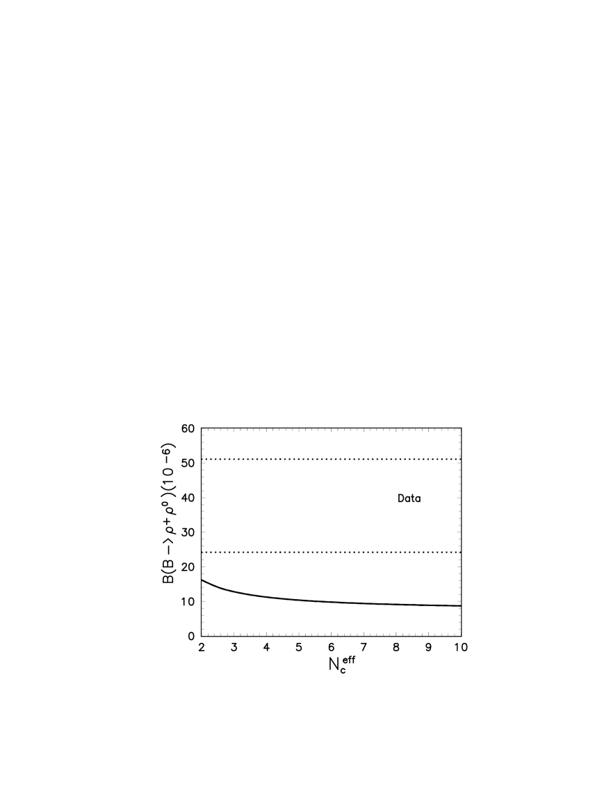
FIG. 3.: Plots of the branching ratio ${\cal B}(B\to\rho^{+}\rho^{0})$ versus $N_{c}^{eff}$ in the SM and the TC2 model for $m_{\tilde{\pi}}=200$ GeV and $N_{c}^{eff}=2-10$, but two curves coincide each other. The band between two dots lines corresponds to the Belle’s measurement: ${\cal B}(B\to\rho^{+}\rho^{0})=(38.5^{+12.6}_{-14.3})\times 10^{-6}$.

FIG. 4.: Plots of the CP asymmetries of $B\to K^{*+}\phi$ and $B\to K^{*0}\phi$ decays versus $N_{c}^{eff}$ in the SM (solid curve) and the TC2 model (short-dashed curve) for $m_{\tilde{\pi}}=200$ GeV and $N_{c}^{eff}=2-10$. The Babar’s limits at $90\%$ C.L. are ${\cal A}_{CP}{(B^{+}\to K^{*+}\phi)}=[-0.88,+0.18]$ and ${\cal A}_{CP}{(B^{0}\to K^{*0}\phi)}=[-0.44,+0.44]$.

REFERENCES

- [1] The BaBar Physics Book, eds. P.F. Harrison and H.R. Quinn, SLAC-R-504 (1998).
- [2] Z.J. Xiao, C.S. Li and K.T. Chao, Phys. Lett. B 473, 148 (2000); Phys. Rev. D 62, 094008 (2000); Phys. Rev. D 65, 114021 (2002); J.J. Cao, Z.J. Xiao and G.R. Lu; Phys. Rev. D 64, 014012 (2001); D. Zhang, Z.J. Xiao and C.S. Li, Phys. Rev. D 64, 014014 (2001).
- [3] G. Buchalla, A.J. Buras and M.E. Lautenbacher, Rev. Mod. Phys. 68, 1125 (1996).
-
[4]
M. Bauer and B. Stech, Phys. Lett. B 152, 380 (1985);
M. Bauer, B. Stech and M. Wirbel, Z. Phys. C 29, 637 (1985); ibid, C 34, 103 (1987). - [5] A. Ali, G. Kramer and C.D. Lü, Phys. Rev. D 58, 094009 (1998).
- [6] H.-Y. Cheng, Phys. Lett. B 335, 428 (1994); B 395, 345 (1997); H.-Y. Cheng and B.Tseng, Phy. Rev. D 58, 094005 (1998).
- [7] D. Du and L. Guo, Z. Phys. C 75, 9 (1997); D. Du and L. Guo, J. Phys. G 23, 525 (1997).
- [8] A. Ali, G. Kramer and C.D. Lü, Phys. Rev. D 59, 014005 (1999).
- [9] Y.H. Chen, H.-Y. Cheng, B. Tseng and K.C. Yang, Phys. Rev. D 60, 094014 (1999).
- [10] M. Beneke, G. Buchalla, M. Neubert and C.T. Sachrajda, Phys. Rev. Lett. 83, 1914 (1999); Nucl. Phys. B 591, 313 (2001); Nucl. Phys. B 601, 245 (2001).
- [11] Y.Y. Keum, H.-nan Li and A.I. Sanda, AIP Conf.Proc. 618(2002)229, and references therein.
- [12] D.S. Du, D.S. Yang and G.H. Zhu, Phys. Lett. B 488, 46 (2000); T.Muta, A.Sugamoto, M.Z.Yang and Y.D.Yang, Phys. Rev. D 62, 094020 (2000); M.Z.Yang and Y.D.Yang, Phys. Rev. D 62, 114019 (2000); D.S.Du, D.S Yang and G.H.Zhu, Phys. Rev. D 64, 014036 (2001); H.Y.Cheng and A.Soni, Phys. Rev. D 64, 114013 (2001); D.S. Du et al., Phys. Rev. D 65, 074001 (2002); Phys. Rev. D 65, 094025 (2002).
- [13] Y.Y. Keum, H.-n. Li and A.I. Sanda, Phys. Rev. D 63, 054008 (2001); Y.Y. Keum and H.-n. Li, Phys. Rev. D 63, 074006 (2001); C.D. Lü, K. Ukai and M.Z. Yang, Phys. Rev. D 63, 074009 (2001).
- [14] S. Weinberg, Phys. Rev. D 13, 974 (1976); D 19, 1277 (1979); L. Susskind, ibid, D 20, 2619 (1979).
- [15] C.T. Hill, Phys. Lett. B 345, 483 (1995);
- [16] G. Buchalla, G. Burdman, C.T. Hill and D. Kominis, Phys. Rev. D 53, 5185 (1996);
- [17] Z.J. Xiao, C.S. Li and K.T. Chao, Eur. Phys. J. C 10, 51 (1999).
- [18] Z.J. Xiao, W.J. Li, L.B. Guo and G.R. Lu, Eur. Phys. J. C 18, 681 (2001).
- [19] D. Atwood and A. Soni, Phys. Rev. D 59, 013007 (1999).
- [20] Z.J. Xiao, C.S. Li and K.T. Chao, Phys. Rev. D 63, 074005 (2001).
- [21] X.-G. He, W.S. Hou, and K.C. Yang, Phys. Rev. Lett. 81, 5738 (1998); I. Hinchliffe and N. Kersting, Phys. Rev. D 63, 015003 (2001).
- [22] CLEO Collaboration, R.A. Briere et al., Phys. Rev. Lett. 86, 3718 (2001); CLEO Collaboration, R. Godang et al., Phys. Rev. Lett. 88, 021802 (2002).
- [23] BaBar Collaboration, B. Aubert et al., Phys. Rev. Lett. 87, 151801 (2001).
- [24] Belle Collaboration, K. Abe et al., Observation of charmless decays and at Belle, LP 2001, Roma, July 23-28, 2001; Belle-conf-0113;
- [25] Belle Collaboration, K. Abe et al., Observation of , Belle-conf-0255.
- [26] BaBar Collaboration, B. Aubert et al., Phys. Rev. D 65, 051101(R) (2002).
- [27] Particle Data Group, K. Hagiwara et al., Phys.Rev. D 66, 010001 (2002).