hep-ph/

SU4252-780/

SU-GP-03/5-1 /

MCTP-03-20

What Can WMAP Tell Us About The Very Early Universe? New Physics as an Explanation of Suppressed Large Scale Power and Running Spectral Index

Mar Bastero-Gil⁽¹⁾, Katherine Freese⁽²⁾ and Laura Mersini-Houghton⁽³⁾

¹ Centre for Theoretical Physics, University of Sussex
Falmer, Brighton BN1 9QJ, United Kingdom
² Michigan Center for Theoretical Physics, Ann Arbor, MI 49109
³ Department of Physics, Syracuse University

The Wilkinson Microwave Anisotropy Probe microwave background data may be giving us clues about new physics at the transition from a “stringy” epoch of the universe to the standard Friedmann Robertson Walker description. Deviations on large angular scales of the data, as compared to theoretical expectations, as well as running of the spectral index of density perturbations, can be explained by new physics whose scale is set by the height of an inflationary potential. As examples of possible signatures for this new physics, we study the cosmic microwave background spectrum for two string inspired models: 1) modifications to the Friedmann equations and 2) velocity dependent potentials. The suppression of low “l” modes in the microwave background data arises due to the new physics. In addition, the spectral index is red ($n<1$) on small scales and blue ($n>1$) on large scales, in agreement with data.

Emails: mbg20@pact.cpes.susx.ac.uk, ktfreese@umich.edu, l.mersini@phys.syr.edu

1 Introduction

The high precision of observational cosmology has placed tight constraints on various cosmological parameters and so far seems to be in excellent agreement with the “concordance model”. The Wilkinson Microwave Anisotropy Probe (WMAP) is an important experiment in this field oriented at measuring the anisotropies in the Cosmic Background Radiation (CBR). Its recent findings [1, 2, 3], especially the suppression of the spectrum at large angular scales and the running of the spectral index, have generated a source of great excitement and speculation [4, 5, 6, 7, 8, 9, 10, 11, 12]. Unfortunately it is difficult to isolate the findings of suppression of low-$l$ modes from cosmic variance limitations. However, we here investigate the possibility that the lack of signal in the temperature angular correlation function on angular scales $\theta\geq 60^{0}$ is a hint of new physics. In addition, there is some indication in the data that the spectral index runs from red on small scales to blue on large scales as compared to a scale invariant spectrum, although the statistical significance of these results is not entirely clear [14, 15, 16]. Both of these effects in the data, the suppression of large scale power and the running of the index, can be explained by new physics.

Some of the recent speculations which attempt to explain the lack of power around $\theta\geq 60^{0}$ involve a finite-size universe with non trivial topology [17, 18, 5] or a closed universe [6, 7, 8]. It is too early to conclude whether these ideas would accommodate the rest of the cosmological data that fit so well with the “concordance model” [19]. Another proposed explanation for the suppressed power on large scales involves double inflation with a period of chaotic inflation followed by new inflation due to a single potential [20, 21].

We take the Universe to remain flat and topologically trivial, and take the point of view that the suppression of the correlations at low multipoles $l\simeq\frac{180}{\theta}$ is providing us with clues about the initial conditions of inflation. More precisely our claim is that from the low “l” suppression of the signal, we could be learning about the initial conditions for the part of inflation that gives rise to observables in structure formation and in the microwave background. The initial conditions for the observable universe could be determined by the new physics, which is the relevant theory valid beyond, and around the cutoff scale $E_{c}$ of effective low energy theories.

Inflationary cosmology [22] was proposed as a solution to the horizon, flatness, oldness, and monopole problems of the standard cosmology. An early epoch of superluminal expansion explains why the universe looks so homogeneous and flat today. We here consider potential-driven models of inflation, in which a potential dominates the energy density of the universe and causes the universe to accelerate. In particular, in models where the height of the potential $V$ is determined by the GUT scale, roughly 60 efoldings of inflation are required to produce a universe that is homogeneous out to the horizon scale. It is only these last $60$ e-foldings of inflation that give rise to the observed structure at present, and the scale of our present Hubble horizon $H_{0}$ would correspond roughly to the $60^{th}$ e-folding before the end of inflation. We here consider models in which physics beyond the inflationary scale (e.g. GUT scale) is modified by the introduction of new physics; this new physics can leave imprints in the CMB at scales near and above the horizon.

Above the $60^{th}$ e-folding the theory is described by new physics. This is the regime corresponding to all the energy scales above $E_{c}$, the cutoff scale of the effective low energy theories. According to this point of view it then follows that the low “l” feature in CBR may originate from the new physics taking place around the initial time of inflation.

The very low $l$ modes in the CBR spectrum at present time, correspond to very large wavelength modes of the order of the current Hubble scale, $H_{0}^{-1}$. Around the e-folding time corresponding to the cutoff scale, these were the first modes to cross the horizon and are the last ones to re-enter at present. Since these modes have been superhorizon sized between inflation and now, they have not been contaminated by the later evolution of the Universe. This means that the information we get from these modes in the primordial spectrum can contain and probe only very early-time effects, which we refer to as pristine information. For this reason we could attribute the new feature observed in the spectrum at low $l$ to the initial conditions of inflation.

Since we use quantum field theory (QFT) and general relativity (GR) as our conventional tools to study and describe inflation, it does not make sense to study inflation and the range of e-foldings corresponding to scales above the cutoff with these tools, as they cease to be valid. Due to the new physics occurring at scales above $E_{C}$, we can not use GR and QFT equations to draw any credible conclusions. For this reason, the e-folding corresponding to the cutoff scale determines the “onset” time for the conventional inflation.

New physics is expected to “kick in” and be important above $E_{c}$, for example string theory. Let us assume that slightly above and around $E_{c}$ there was a period where some kind of unknown transition took place. This transition is needed to smoothly bridge the end of the string regime at (which we are taking here to be the fundamental high energy theory), to the epoch of the conventional “lower” energy inflation $V<E_{c}$, as described by QFT and GR formalisms.

As specific examples of new physics above the scale $E_{c}$, we consider two modifications to the formalism of standard cosmology: 1) the effective Friedmann equation receives stringy corrections [23, 24, 25, 26]; or 2) the inflaton potential is velocity dependent due to relative brane motion [27]. Certainly, once inflation starts, after a few e-folds our patch of spacetime has inflated sufficiently, that the “string era” becomes an irrelevant description and we enter/recover the conventional cosmology period of the standard model (see, e.g., [28]). That is to say, that GR and QFT, soon after the transition from the string era, should be recovered in the low energy limit.

As our first example, we consider modifications to the Friedmann equation,

$$H^{2}={8\pi\over 3M_{P}^{2}}\left(\rho+f[\rho^{\alpha}]\right),$$ (1)

where $\rho$ is the energy density, $\alpha$ is a parameter, and $f$ indicates the modification term to the Friedmann equation. The second term is important in the regime $\rho\geq\sigma$ where $\sigma$ is an energy scale, introduced by the underlying string model, to be defined below. In particular, we focus on the model of Randall and Sundrum (hereafter RSI) that was proposed as an explanation of the hierarchy problem [29]. Here our observable universe is a three-dimensional surface situated in extra dimensions. During the inflationary epoch, the Friedmann equation on our 3-brane becomes

$$H^{2}={8\pi\over 3M_{P}^{2}}[\rho+\frac{\rho^{2}}{2\sigma}],$$ (2)

where $\sigma$ is the brane tension. Recall that in the original Randall-Sundrum model the brane tension has to be negative in order to ensure stability of the bulk. Previous authors  [31, 32] have considered inflation in the presence of such a second term, but focused on the case of a positive tension $|\sigma|<<V$, with $V$ the energy scale of the inflaton potential. They found that the extra contribution to the Hubble expansion helps damp the rolling of the scalar field so that the condition for slow-roll inflation can be met even for a steep potential. Here on the other hand, we are interested in a very different regime, with a mass scale

$$|\sigma|^{1/4}\sim V^{1/4}\sim[10^{-3/4}M_{P}].$$ (3)

The reason for this choice for $\sigma$ is that, in many inflationary models, the height of the potential is given by the GUT scale. Thus the second term in Eqn. (2) will be important at the “onset” of inflation, $\phi_{i}\simeq O(M_{P})$, exactly for this choice of the brane tension, $\sigma\simeq V$. As shown by  [33], inflationary potentials must be flat in the sense that the ratio of the height of the potential to the fourth power of the width must satisfy

$$\Delta V/(\Delta\phi)^{4}\leq O(10^{-7});$$ (4)

this statement quantifies what is often known as the “fine-tuning” problem in inflation. For $\Delta\phi\sim M_{P}$, then one needs $V\leq 10^{-2}M_{P}^{4}$.

Such a parameter choice is plausible for the model of Randall and Sundrum  [29]. In RSI, the four and five dimensional Planck scales $M_{P}$ and $M_{5}$ respectively are related via

$$M_{P}^{2}=(3/4\pi)\left({M_{5}^{2}\over|{\sigma}|}\right)M_{5},$$ (5)

where $\sigma$ is the brane tension and is negative. With Eqn. (3) and taking $M_{P}=10^{19}$ GeV, we require

$$M_{5}^{3/2}\sim M_{P}/20,$$ (6)

a reasonable value. Here we are studying a situation in which, due to “stringy” effects, the effective Friedmann equation is modified above the scale $\sigma$ for the inflaton potential $V$ but returns to normal soon after.

We will show that the density fluctuations well below today’s horizon scale are not significantly altered, while fluctuations on large scales (near the horizon scale) are substantially suppressed. The perturbations produced on the large scales near the horizon are produced close to the scale of new physics. The role of the new physics is to cause the breakdown of the slow-roll approximation. At the very earliest times, the kinetic energy of the inflaton field dominated over the potential. Hence at these early times, density fluctuations were not produced in the usual way. Eventually the potential does come to dominate the energy density. Once the potential drops to the scale $V\sim\sigma$, slow roll inflation ensues. This transition happens roughly 60 efoldings before the end of inflation. Smaller scale fluctuations are produced during the slow-roll phase of inflation, where the height of the potential is fairly constant, so that the slope of the power spectrum is only mildly affected.

This proposed explanation of the suppression of large scale power in the WMAP data relies on the fact that the scale of new physics $E_{c}=\sigma^{1/4}$ exactly corresponds to the height of the inflationary potential at 60 efolds before the end of inflation. This is the only fine-tuning that is required. Once this energy scale is set, then it is automatic that kinetic energy domination suppresses large scale perturbations at exactly the right angular scale, namely just below the horizon. The fine-tuning need not be severe, e.g, in the sense that the required ratio of four and five dimensional Planck scales in Eqn. (6) is not unreasonable.

A similar proposal by [9] also invokes the failure of slow-roll at 60 e-folds before the end of inflation. In that paper, the authors proposed a change in shape of a hybrid inflation potential exactly at the right time to obtain the large scale suppression. The fine-tuning there is of a different nature. The paper of [9] requires the potential or the initial conditions to be carefully chosen. In this paper, on the other hand, we do not require any special features of the potential, which can indeed be quite ordinary. Instead, the violation of slow-roll arises due to modifications e.g. to the Friedmann eqn. It would be interesting to consider the question of how to differentiate observationally between these different proposals.

In addition, the new physics changes the running of the spectral index. We will show that an oddity of the data, namely that the index is red ($n<1$) on small scales and blue $(n>1)$ on large scales is automatically explained in the model we study.

We demonstrate in Section 2 how two types of modifications that generically arise in string theory, those with modified Friedman equation and those containing velocity dependent inflaton potentials, may leave important imprints in the primordial spectrum. We also show the result generated with the CMBFAST program, that convert the primordial spectrum, $\delta_{H}$ where these signatures are imprinted, to a present-day power spectrum, $P(k)$ and accompanying anisotropies in the CBR. The resulting anisotropies for two representative examples are then compared with WMAP data. These are summarised in Section 3.

2 String correction effects on the primordial spectrum

Let us assume that, due to the underlying theory valid at high energies, for example string theory, the Einstein equations receive corrections. Some familiar examples can be found in brane-world scenarios which generically either modify Einstein equations  [23, 24, 25, 26, 34] or contain a velocity dependent term in the inflaton potential [27]. This velocity dependent term, related to the relative brane motion, can also be recast as a modification to the Friedmann equation and is calculable in string theory. We know that at later times general relativity is a perfectly valid theory and hence, we expect these corrections to be important and play a role only at early times, during the transition from a string theory era to the onset of the standard brane-bound $3-dimensional$ inflation. Within very few e-foldings during inflation, our patch of spacetime becomes large enough and these modifications become negligible.

Here we are interested in addressing the following issue: Do stringy corrections leave any imprint in the primordial power spectrum, and at what scales would we expect to see this signature?

2.1 The Spectrum for the Modified Friedmann Equation from Brane-Worlds

Initially, let us consider the corrections to be of a general form $f[\rho^{\alpha}]$, i.e.,

$$H^{2}=\frac{8\pi}{3M_{P}^{2}}\left(\rho+f[\rho^{\alpha}]\right)\,,$$ (7)

where $\rho$ is the inflaton energy density and $\alpha$ is a parameter. Energy conservation requires

$$\dot{\rho}+3H(\rho+p)=0\,,$$ (8)

where $p$ is the pressure and “dot” denotes the derivative with respect to cosmic time. The acceleration equation for the scale factor $a$ is

$$\frac{3M_{P}^{2}}{4\pi}\left(\frac{\ddot{a}}{a}\right) = \frac{3M_{P}^{2}}{4\pi}\left(\dot{H}+H^{2}\right)=-\left(\rho+f[{\rho}^{\alpha}]+3p+3p_{f}\right)\,,$$ (9)

where $p_{f}$ would be an “effective” pressure contribution due to the modification to the energy density in the Friedmann equation:

$$p_{f}=(\rho+p)\frac{df[\rho^{\alpha}]}{d\rho}-f[\rho^{\alpha}]\,.$$ (10)

Given the above setup, let us proceed in calculating the primordial spectrum $\delta_{H}(k)$ for the case when the Friedmann equation contains corrections of the form Eqn. (7), that were introduced by the new high energy physics around the cutoff scale. The symbol $\delta_{H}(k)$ denotes the primordial spectrum which gives the amplitude of perturbations as the comoving wavenumber $k$ enters the horizon. $P(k)$ denotes the present-day power spectrum giving us the amplitude of perturbation at a fixed given time. They are related by the transfer function $T(k)$  [35], for the present Hubble value $H_{0}$,

$$\frac{k^{3}}{2\pi}P(k)=\left(\frac{k}{aH_{0}}\right)^{4}T^{2}(k)\delta_{H}^{2}(k)\,.$$ (11)

We will follow the standard approach to calculating the density (curvature) perturbations created during inflation, but will make the appropriate modifications required by Eqn. (7). During inflation, when the inflaton $\phi$ with energy $\rho\simeq V$ is the dominant one, the primordial power spectrum $\delta_{H}(k)$ is

$$\delta_{H} \simeq \left(\frac{\delta\rho}{\rho+p}\right)_{k=aH}\,,$$ (12)

where,

$$\delta\rho \simeq \delta\phi V^{\prime}\simeq\frac{H}{2\pi}V^{\prime}\,,$$ (13)

$$\rho+p \simeq -[\frac{M_{P}^{2}}{4\pi}\dot{H}+f[\rho^{\alpha}]+p_{f}]\,,$$ (14)

with $V^{\prime}=dV/d\phi$. Henceforth, throughout the remainder of this section, all quantities in the equations will be evaluated at horizon crossing, i.e., at $k=aH$. Therefore,

$$\delta_{H}\simeq\left(\frac{H}{2\pi}\right)\left(\frac{-V^{\prime}}{\frac{M_{P}^{2}}{4\pi}\dot{H}+f[\rho^{\alpha}]+p_{f}}\right)\,.$$ (15)

When the modification term $f[{\rho}^{\alpha}]$ is non-negligible, clearly $\delta_{H}$ “feels” the effect of “the stringy” corrections.

The spectral index $n_{S}$ can readily be found from the primordial spectrum, Eqn. (15)

$$n_{S}-1=\frac{d\ln\delta_{H}^{2}}{d\ln k}\,,$$ (16)

where the k-dependence of the spectrum is

$$\delta^{2}_{H}\propto\left(\frac{k}{k_{S}}\right)^{n_{S}-1}\,,\,.$$ (17)

with $k_{S}$ a fiducial wavenumber depending on the dynamics of inflaton.

The latter expression for the primordial spectrum in terms of $k$ Eqn. (17), can be derived from Eqn. (15) by replacing in the solution for $\phi(t)$, the time dependence of the field with the comoving momentum $k$, through the condition $k=a(t)H$ and $a(t)=e^{N_{e}}$, with $N_{e}=$ number of e-folds.

In the remainder of this section, we will present a rough estimate of how density fluctuations may be modified due to the presence of an energy cutoff in the spectrum given by $E_{c}$. Then in the following sections, we will present precise examples in which we calculate exactly the resultant power spectrum. The rough arguments in the remainder of this section give a good general idea of our results.

Let us denote the unmodified power spectrum by $\delta_{H}^{0}$ and the unmodified spectral index by $n_{S}^{0}$, obtained by the limit $f[\rho^{\alpha}]\rightarrow 0$. We can re-express the corrections in the modified spectrum in Eqn. (15) and the running of the spectral index as a function of the weighted wavenumber $k/k_{S}$.

$$\delta^{2}_{H}=\delta^{(0)2}_{H}\frac{1}{(1+4\pi(f[\rho^{\alpha}]+p_{f})/(M_{P}^{2}\dot{H}))^{2}}\propto\left(\frac{k}{k_{S}}\right)^{n_{S}-1}\,,$$ (18)

with $\delta_{H}^{(0)2}$ given in term of $n_{S}^{0}$

$$\delta^{(0)2}_{H}\propto\left(\frac{k}{k_{S}}\right)^{n^{0}_{S}-1}\,.$$ (19)

Let us denote the term in brackets which is next to $\delta_{H}^{(0)2}$ in Eqn. (18) by

$$g(\phi)=\frac{1}{(1+4\pi(f[\rho^{\alpha}]+p_{f})/(M_{P}^{2}\dot{H}))^{2}}\,.$$ (20)

Differentiating with respect to $\ln k$ the correction to the spectral index is

$$(n_{S}-1)=(n^{0}_{S}-1)+\left(\frac{d\ln g(\phi)}{d\ln k}\right)=(n^{0}_{S}-1)+\delta n_{S}\,.$$ (21)

Therefore the correction term $\delta n_{S}$ is given by

$$\delta n_{S}=n_{S}-n_{S}^{(0)}=\left(\frac{d\ln g(\phi)}{d\ln k}\right)=\left(\frac{d\ln g(\phi)}{d\phi}\right)\left(\frac{d\phi}{d\ln k}\right)=\frac{g(\phi)^{\prime}}{g(\phi)}\frac{\dot{\phi}}{H}\,,$$ (22)

where $d\phi/d\ln k=\dot{\phi}/H$ (evaluated at horizon crossing, $k=aH$). Note that since $g(\phi)$ is a function of $\phi(t)$ then the correction $\delta n_{S}$ is generically a function of $k$. Its k-dependence can be estimated in the same manner as we calculate $\delta_{H}(k)$, by replacing the time dependence of the field in favour of $k$ at $k=aH$.

Formally, the $k$- dependence of $g(\phi)$ as a function of $\delta n_{S}$, in a similar manner to $\delta_{H}$, is expressed by

$$g(\phi)=\left(\frac{k}{k_{S}}\right)^{\delta n_{S}(k)}\,.$$ (23)

Depending on the model and the specific form of the modification function $g(\phi)$, it should be noted that for certain values of $k$ the correction term, $\delta n_{S}(k)$ may become large and thus the slow roll conditions may be violated, as illustrated in Sec.(2.3).

But at $k\leq k_{S}$, we can recast Eqn. (23) in the form

$$g(\phi)\propto\left[1-e^{-(\frac{k}{k_{S}})^{\delta n_{S}}}\right].$$ (24)

The modified spectrum, with $\delta n_{S}$ given by Eqn. (22), becomes

$$\delta^{2}_{H}=\delta^{(0)2}_{H}\left[1-e^{-(\frac{k}{k_{S}})^{\delta n_{S}}}\right]\,.$$ (25)

In Fig. (1) we show as an example the result generated with the CMBFAST program, that convert the primordial spectrum to a present-day power spectrum. We show for comparison the resulting anisotropies for an unmodified primordial spectrum $\delta_{H}^{(0)}$, with $n_{S}^{(0)}=0.99$, and the modification as given in Eqn. (25), with the choice of parameters $\delta n_{S}=1$ and $k_{S}=0.0005\,Mpc^{-1}$. We allowed all the parameters to be the conventional ones of a $\Lambda$CDM universe, with matter density $\Omega_{M}=0.27$, vacuum energy density $\Omega_{\Lambda}=0.73$, baryons $\Omega_{b}=0.046$, and $H_{0}=71{\rm kms}^{-1}{\rm Mpc}^{-1}$. We note a very similar study to Fig. (1) [9] appeared during the course of our work on this paper.

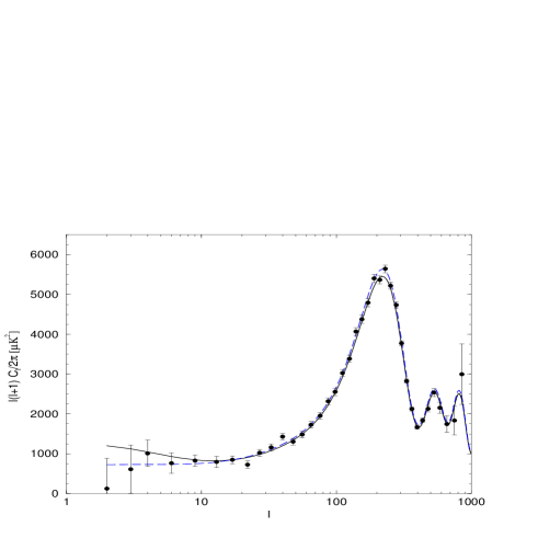
Figure 1: CBR spectrum of anisotropies with the modified primordial spectrum given in Eqn. (25), with $\delta n_{S}=1$, and $k_{S}=0.0005\,Mpc^{-1}$. We also show for comparison the curves for the standard spectrum Eqn. (19), with $n_{S}^{(0)}=0.99$. Cosmological parameters as given by the best fit model of the WMAP collaboration.

2.2 The Spectrum for the Velocity Dependent Inflaton Potentials from String Theory

The second class of modifications generically derived from string theoretical inflationary models involves a velocity dependence in the potential $V(\phi)\propto\frac{\dot{\phi}^{p}}{\phi^{q}}+constant$ for the inflaton field $\phi$. In string theory this term shows up and is non negligible when branes move with respect to each other.

These models were treated in  [27] by absorbing the velocity dependent modification $Z(\phi)$ into the definition of the potential and the slow roll parameters. The effective action for the inflaton in this case is

$$\Gamma(\phi)=\int d^{4}x\left(-a^{3}V(\phi)+\frac{1}{2}a^{3}Z(\phi)\dot{\phi}^{2}-\frac{1}{2}aZ(\phi)(\nabla\phi)^{2}\right)\,.$$ (26)

The reader can find all the details of the calculation of the modified primordial spectrum in  [27]. Here we will just report their expression for $\delta_{H}$ in terms of the unmodified spectrum $\delta^{0}_{H}$, (the latter is obtained by the limit $Z(\phi)\rightarrow 1$), and the stringy modification term $Z(\phi)$,

$$\delta_{H}=\delta^{0}_{H}Z(\phi)\,.$$ (27)

Therefore the running of the spectral index is given by

$$\delta n_{S}=n_{S}-n^{0}_{S}=2\frac{d\ln Z}{d\ln k}\,.$$ (28)

Clearly by comparing this class of velocity dependent modifications with the modified Friedmann equation of the previous subsection, the effect of $Z(\phi)$ in the spectrum is identical to that of $g(\phi)$. The running of the spectral index is such that if the slow roll conditions persist in the presence of stringy modifications, $|\delta n_{S}|<1$. Notice that $\delta n_{S}$ is a function of the energy scale $k$ and runs with $k$ through its dependence on $V$,$V^{\prime}$, $Z$, $Z^{\prime}$, $f$, $f^{\prime}$. For example, if we are deep into the regime of new physics $V>E_{c}$, it is possible that these modifications are strong enough to break the slow-roll conditions thus one would get a different $|\delta n_{S}|\geq 1$ answer, if backreaction of stringy terms violates the slow-roll regime as we show below with two examples.

Since we are interested in the k-dependence of the modifications in the primordial spectrum one can do the same algebraic tricks in order to express the modifications in the spectrum as

$$Z(\phi)^{2}=\left(\frac{k}{k_{S}}\right)^{\delta n_{S}}\propto[1-e^{-(\frac{k}{k_{S}})^{\delta n_{S}}}]\,.$$ (29)

The authors of  [27] made the important observation that one possible signature of string models is the fact that tensor perturbations are not affected by these modifications, therefore the ratio of tensor to scalar perturbations will be different from the unmodified inflationary models. This is due to the different origins of tensor fluctuations arising from bulk modes versus scalar perturbations arising from brane quantum fluctuation modes. In this work we are offering a new way for detecting signatures of the string theoretical brane world models, through the suppression effect they induce on the power spectrum at very low “l”.

2.3 Examples

Modifications of Friedmann equation for the Randall Sundrum type of brane-worlds

In this scenario [29] the modification to the Friedmann equation for the brane bound observer [23, 24, 25, 26, 34] is

$$H^{2}={\Lambda_{4}\over 3}+\left({8\pi\over 3M_{P}^{2}}\right)\rho+\left({4\pi\over 3M_{5}^{3}}\right)^{2}\rho^{2}+{\epsilon\over a^{4}},$$ (30)

where $\epsilon$ is an integration constant that appears as a form of “dark radiation” that is not important during inflation. We will also assume that the bulk cosmological constant $\Lambda\sim-4\pi\sigma^{2}/3M_{5}^{3}$, so that the three-dimensional cosmological constant $\Lambda_{4}$ is negligible during the early universe. Hence the relevant correction to the Friedmann equation during inflation is the quadratic term,

$$f[\rho^{\alpha}]=\rho^{2}/2\sigma\,,$$ (31)

so that

$$H^{2}={8\pi\over 3M_{P}^{2}}\rho[1+\rho/2\sigma]\,,$$ (32)

with the cutoff scale given by the brane tension,

$$E_{c}\sim|\sigma|.$$ (33)

Notice that in the absence of bulk fields, $\sigma<0$ in order to ensure stability. As can be seen from Eqn. (15) we have a suppression of power when the modification term is significant at early times. One recovers the conventional spectrum at later times when the modification term becomes negligible.

$$\left\{\begin{array}[]{ll}\delta_{H}<\delta_{H}^{(0)}&\mbox{when}\;\;\;\;\rho^{2}/|\sigma|\geq\rho\,,\\ &\\ \delta_{H}\rightarrow\delta_{H}^{(0)}&\mbox{when}\;\;\;\;\rho^{2}/|\sigma|<\rho\,.\end{array}\right.$$ (34)

Under the slow roll conditions $\rho\propto V$, Eqn.(32) becomes

$$H^{2}={8\pi\over 3M_{P}^{2}}V\,\left[1-{V\over 2|\sigma|}\right]\,,$$ (35)

and the expression for $\delta_{H}^{2}$ can be derived by using Eqns. (20 -22):

$$\delta n_{S}(k)=\frac{-V^{\prime 2}}{3H^{2}(V-2|\sigma|)}=\frac{9\dot{\phi}^{2}}{(2|\sigma|-V)}\,.$$ (36)

We note that an equivalent expression to Eqn. (15) has been derived previously  [31] in the slow roll regime.

$$\delta_{H}^{2}\sim\bigl{(}{512\pi\over 75M_{P}^{6}}\bigr{)}{V^{3}\over{V^{\prime}}^{2}}\left[1-{V\over 2|\sigma|}\right]^{3}.$$ (37)

However, the slow roll assumption breaks down at early times due to the new physics modifications. In this example, if we extrapolate backwards to a value $\phi_{*}$ of the inflaton field at which $V(\phi_{*})=2|\sigma|$, we have $\delta n_{S}\rightarrow\infty$ and $\delta_{H}^{2}\rightarrow 0$. Therefore near the critical point $\phi_{*}$, the calculation for the spectrum should be done by using Eqn. (15) instead of Eqn. (37) since the approximation $\dot{\phi}\simeq-V^{\prime}/3H$ breaks down.

At the high energy scales (early times) at which the slow roll approximation breaks down, the energy density is dominated by the kinetic energy of the inflaton, and density fluctuations are not produced. So this effect is imprinted in low $l$ since these modes are the first to cross the horizon at the initial time. However, we need to translate the suppression of these wavenumbers into the “spreading” that this feature has over the range of “l’s” in the present day power spectrum, $P(k)$, as seen in Fig.2.

The magnitude of suppression is of course model dependent and it is a function of our assumptions about the modification term $V^{2}/(2\sigma)$ and the energy scales for $V$, $|\sigma|$ which we took to be $GUT$ scale here.

For the sake of concreteness, let us assume the following inflaton potential  [36, 37],

$$V=V_{0}e^{-\lambda\phi}\,,$$ (38)

(where $\phi=\Phi/\sqrt{8\pi}M_{P}$ is the inflaton field given in Planck units in order to be dimensionless). We shift the field so that its initial value at 60 efolds before the end of inflation is at $\phi_{i}=0$. Then the solution for the inflaton field in the presence of modifications becomes

$$\phi=\frac{\lambda}{(1-\frac{V_{0}}{2|\sigma|})}\ln(\frac{aH}{a_{i}H_{i}})_{k=aH}\sim-\lambda\,\,\Delta N\,\,{1\over(1-{V_{0}\over 2|\sigma|})}\,,$$ (39)

where

$$\Delta N=N_{I}(k)-N_{I}(k_{s})=\ln({k_{s}\over k})\,,$$ (40)

and $N_{I}(k)$ is the number of efoldings before the end of inflation at which perturbations on scale $k$ leave the horizon. The spectral index obtained in the usual exponential inflation case without modified Friedmann equations is given by $n^{0}_{S}-1=-\lambda^{2}$.

By replacing the field solution we obtain

$$\tilde{g}(\phi) = [1+\frac{V}{2\sigma}]^{3}\,=\,[1-\frac{V_{0}}{2|\sigma|}\,(\frac{k}{k_{S}})^{\frac{(n^{0}_{S}-1)}{(1-\frac{V_{0}}{2|\sigma|})}}]^{3}\,,$$ (41)

and

$$\delta_{H}^{2}\sim 8\pi\bigl{(}{512\pi\over 75M_{P}^{4}}\bigr{)}\,\,{V_{0}\over{\lambda}^{2}}\left[\frac{k}{k_{S}}\right]^{\frac{(n^{0}_{S}-1)}{(1-\frac{V_{0}}{2|\sigma|})}}\,\,{\tilde{g}(\phi)}.$$ (42)

which produces the suppression feature in the low “l” regime, corresponding to $V_{0}\simeq|\sigma|$, i.e the regime where new physics becomes important. Here, $k_{S}$ corresponds to the scale of perturbations produced 60 efoldings before the end of inflation, which corresponds to the horizon size today, $k_{S}\sim(4000Mpc)^{-1}$.

In Figure 2, we present the results obtained using the CMBFAST code with the modifications of Eqns. (41) and (42) for two different values of $\lambda$ and of $k_{S}$, with the height of the potential determined by $|\sigma|\sim M_{GUT}\sim 10^{16}$GeV. In the plot, we have chosen to normalize all the curves to the value of the WMAP $l=17$ multipole for comparison. In order to match the amplitude of the data, we choose values of $\lambda^{2}\sim 0.1$ as shown in the plot. We see that the Doppler and higher peaks can be essentially unaffected by these modifications, while the low $l$ modes are substantially suppressed. Hence the WMAP data is better fit by these modifications than by a standard $\Lambda$-CDM model. We have not performed a quantitative study in this paper of how good the fit is to the data, which for a particular model may be the subject of future work; it is our goal here to display the possible role of new physics in the suppression of low “l” modes.

In order to illustrate the role of modifications, let us start in the slow roll regime, where Eqn. (35) is valid, and go backwards in time (up the potential). At first, as we climb up the potential, the value of the Hubble constant $H$ increases. Then, when we reach the value of $\phi$ at which $V(\phi)=|\sigma|$, we see that we have reached a maximum for $H$, i.e., $\delta H/\delta V=0$. In other words, $H$ is maximized for $V=|\sigma|$. When we continue to climb up the hill, $H$ decreases towards zero, and the slow roll approximation begins to fail as the kinetic energy of the inflaton becomes more and more important. At $\rho(\phi_{*})=2|\sigma|$ the spectrum $\delta_{H}\rightarrow 0$, $n_{S}\rightarrow\infty$, thus signalling a completely stringy regime and the slow roll conditions being badly violated. Notice that modifying the Hubble parameter, $H$ through the “stringy terms”, changes the kinetic energy of the inflaton, since $H$ play the role of a friction term for the field.

Let us parametrize the kinetic energy of the inflaton as $K=\frac{\dot{\phi}^{2}}{2}=\alpha V$. Slow roll requires that $\alpha\leq 1/2$. Then the inflaton energy density is $\rho(\phi)=(1+\alpha)V(\phi)$. The value of the field $\phi_{*}$ for which the modified Hubble parameter vanishes $H=0$, is given by the solution $\phi_{*}\simeq\frac{1}{\lambda}\ln[(\frac{2|\sigma|}{V_{0}})(\frac{1}{1+\alpha_{*}})],(1+\alpha_{*})\leq 3/2$. At $\phi=\phi_{*}$ where $H=0$ the inflaton has a lot of kinetic energy. But when the field rolls at some $\phi_{i}$ given by $\rho(\phi_{i})\simeq O(|\sigma|)$ we have the start of the slow-roll regime with the kinetic energy of the inflaton decreasing to less than $V(\phi_{i})/2$. For field values between $\phi_{i}>\phi>\phi_{*}$ the “friction term” $H$ starts increasing and the kinetic energy of the inflaton decreases. The point where the field acquires the value $\phi_{i}\simeq\frac{1}{\lambda}\ln[(\frac{|\sigma|}{V_{0}})(\frac{1}{1+\alpha_{i}})]$ is a maximum for $H^{2}(\phi)$. Clearly $\alpha_{i}\ll\alpha_{*}\leq 1/2$. In the region of the validity of new physics, due to the modified friction term $H$ for the field, i.e. for $\phi_{i}\geq\phi\geq\phi_{*}$, the inflaton was in a “fast-roll” since its kinetic energy was large due to the highly suppressed modified “friction term” $H$. Therefore all long wavelength perturbations are highly suppressed in this regime. However as the modified Hubble parameter increases towards $\phi=\phi_{i}$ and attains its maximum at $\phi_{i}$ then the kinetic energy of the inflaton starts decreasing until it reaches a minimum at $\phi_{i}$. At $\phi_{i}$ its potential energy $V(\phi_{i})\simeq|\sigma|$ dominates over the kinetic term and the inflaton enters the slow-roll regime of a conventional inflationary period, even in the presence of a modified Hubble parameter. The Hubble parameter and $V(\phi)$ slowly decrease for the standard model regime of the slow roll, $\phi_{end}\geq\phi\geq\phi_{i}$ thus rendering the stringy correction terms insignificant in this range of $\phi$.

In short, modified Friedmann equations of RSI provide a possible explanation of suppressed large scale power in the WMAP data, for parameter choices such as those shown in Figure 2.

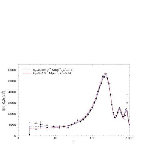
Figure 2: CBR spectrum of anisotropies with the modified primordial spectrum for the Randall Sundrum example, Eqn. (41), with $V_{0}\simeq|\sigma|\sim m_{GUT}$; $k_{S}=0.0005\,Mpc^{-1}$ (dashed line) and $k_{S}=0.00024\,Mpc^{-1}$ (dot-dashed line). We also show for comparison the curve for the standard spectrum Eq (19), with $n_{S}^{(0)}=0.99$ (solid line). Cosmological parameters as given by the best fit model of the WMAP collaboration.

Running Spectral Index

The WMAP data show some evidence that the spectral index $n_{s}$ runs (changes as a function of the scale $k$ at which it is measured) from $n_{s}>1$ (blue) on large scales to $n_{s}<1$ (red) on small scales. Chung, Shiu and Trodden [12] proposed that such a running index may be obtained in inflationary models if the slope of the potential reaches a minimum in the regime where the spectral behavior changes; such a potential must be carefully chose. In another proposal [38, 39], an inflationary model motivated by supergravity was proposed as an explanation of the running spectral index, in which a period of hybrid inflation is followed by a second period of inflation. We here propose an alternate possibility for explaining the running spectral index.

We will see that the density perturbations from modified Friedmann equations in Eqn.(42) (although not described in terms of an overall spectral index) give rise to a spectrum that is blue on large scales and red on small scales, in agreement with the WMAP data. We find that $\delta_{H}^{2}$ is an increasing function of $k$ for small scales, and a decreasing function for large scales. We find that $\delta_{H}^{2}$ reaches a maximum at

$$k_{max}/k_{s}=\left[{|\sigma|\over 2V_{0}}\right]^{{1\over\tilde{n}-1}}$$ (43)

where

$$\tilde{n}-1={\frac{(n^{0}_{S}-1)}{(1-\frac{V_{0}}{2|\sigma|})}}.$$ (44)

For $V_{0}=|\sigma|$ and taking $\lambda^{2}=0.11$ as in Fig.(2), we find that $k_{max}/k_{s}=23$ so that the maximum power is on scales of roughly 180 Mpc. The power decreases as one moves away from the maximum in either direction. Hence, compared to a flat spectrum, the spectral index is shifted to the red on small scales and blue on large scales.

Hence modified Friedmann equations have the capability of explaining not only the suppression of power on the scales of the quadrupole, but also the running of the spectral index observed in the data.

Velocity dependent potentials from string theoretical inflationary models

As mentioned in Section 1, the cosmological consistency conditions for this class of modifications were treated in great detail in  [27]. In our work we are interested to search for possible low “l” signatures that this class of models may give rise to, thus presenting this class of stringy modifications as a second example. In order to illustrate our point, let us consider the following velocity dependent modification as a representative example for this class

$$Z(\phi)=1-V(\phi)/E_{c}\,.$$ (45)

Post Newtonian corrections of higher dimensional gravity are also expected to give rise to such modification terms. In this case the correction power is given by

$$\delta n_{S}=(2/Z)(dZ/d\phi)(\dot{\phi}/H)=\frac{2V^{\prime 2}}{3H^{2}E_{c}(1-\frac{V}{E_{c}})^{2}}\,.$$ (46)

In the regime where the slow roll condition is valid, $\delta n_{S}<1$ and therefore we can approximate the modification term in the primordial spectrum by an exponential. The modified primordial spectrum will then be given by Eqn. (25) with $\dot{\phi}\simeq\frac{-V^{\prime}}{3HZ}$.

If we now take $V=V_{0}e^{\lambda\phi}$ as in the previous case, this class of modifications is another example whereby we again obtain a suppression of the signal at low “l” through

$$\delta n_{S} = 2\,\lambda^{2}\,(V_{0}/E_{c})(\frac{k}{k_{S}})^{\frac{\lambda^{2}}{[1-(V_{0}/E_{c}]}}\,\,\frac{1}{[1-(V_{0}/E_{c})(\frac{k}{k_{S}})^{\frac{\lambda^{2}}{[1-(V_{0}/E_{c}]}}]^{2}}\,,$$ (47)

Again this correction term blows up at $V_{0}=E_{C}$ thus violating slow-roll and introducing a cutoff on the spectrum $\delta_{H}\simeq 0$ at the energy scale $V(\phi_{*})=E_{c}$. Hence the period of fast roll is due to the modified friction term $H$ for the inflaton at high energies, $V\simeq O(E_{c})$, and it comes to an end when the Hubble parameter, due to the rolling field, goes through its saddle point extremum at $V(\phi_{i})\simeq\frac{E_{c}}{2},\phi_{i}\simeq\frac{1}{\lambda}\ln(E_{c}/2V_{0})$. This is also the point where the kinetic energy of the inflaton drops by more than half its potential energy and the inflaton enters into the slow roll phase from this point onwards. Also since $V(\phi_{end})\ll V(\phi_{i})\ll V(\phi_{*})$ the correction terms soon become small when the field enters the phase of the standard physics regime, for $\phi\leq\phi_{i}$.

It should be noticed that the initial condition and the start of the slow-roll regime at $\phi_{i}$, in both examples, result from and are fixed by the stringy correction term of the new physics because this modification determines the saddle point location for the “friction term” of the field, namely the Hubble parameter $H$. Thus the model-dependence can not be avoided in the absence of knowledge of the fundamental theory of new physics. However, observational data ought to discriminate between the various theoretical models for the high energy regime.

3 Summary

The new results for the suppression of the low order multipoles in the microwave background spectrum, measured by the Wilkinson Microwave Anisotropy Probe mission, are very intriguing. They may give us clues towards new physics that determines the initial conditions for inflation. As examples of new physics that may be responsible for this deviation we investigate modified Friedmann equations and velocity dependent potentials, that may have resulted from a deeper underlying theory, for example string theory. Using the CMBFAST code we see that indeed fundamental new physics can give rise to the feature observed by WMAP at low “l”. However the type of feature produced is determined by the model chosen for the stringy modifications at high energies, as we illustrated with the examples of Sec. 2 above. The important issue, as we have shown in this work, is that the low “l” signatures in the CBR spectrum would offer another piece of evidence for testing string cosmology and our assumptions about the initial conditions of inflation originating from new physics. In addition, these modifications to the basic physics have the capability of explaining not only the suppression of power on the scales of the quadrupole, but also the running of the spectral index observed in the data. It is exciting that ideas about new physics and the initial conditions may be testable and within observational reach.

In some cases, the stringy modifications may become important once more, at very recent times. An example is the class of string inspired models that contain late time effects in the form of dark energy [40, 41, 42, 43, 44]. A very interesting relation exists in that case between the two apparent coincidences around redshifts $z\leq 1$, dark energy domination and the low “l” suppression; however, we will report on this scenario in a separate publication.

ACKNOWLEDGMENTS: We would like to thank S.Carroll, C. Csaki, P. Greene, W. Kinney, J. Liu, M. Trodden, G. Shiu, G. Starkman and R. Sorkin, for helpful conversations. LM’s work is supported is supported in part by the U.S. Department of Energy under grant DE-FG02-85ER40231 and by the National Science Foundation under grant PHY-0094122. KF acknowledges support from the Department of Energy through a grant at the University of Michigan; KF also thanks the Michigan Center for Theoretical Physics for support.

References

- [1] C.L. Bennett et al., astro-ph/0302207; G. Hinshaw et al., astro-ph/0302217.
- [2] D.N. Spergel et al., astro-ph/0302209.
- [3] II.V. Peiris et al., astro-ph/0302225.
- [4] A. Berera, L. Z. Fang and G. Hinshaw, Phys. Rev. D 57 (1998) 2207; A. Berera and A. F. Heavens, Phys. Rev. D 62 (2000) 123513.
- [5] M. Tegmark, A. de Costa-Oliviera, A. Hamilton, astro-ph/0302496; J.-P. Uzan, A. Riazuelo, R. Lehoucq and J. Weeks, astro-ph/0303580.
- [6] G. Efstathiou astro-ph/03303127; S. L. Bridle, A. M. Lewis, G. Efstathiou, astro-ph/0302306.
- [7] J.-P. Uzan, U. Kirchner, G. F. R. Ellis, astro-ph/0302597.
- [8] A. Linde, astro-ph/0303245.
- [9] C. R. Contaldi, M. Peloso, L. Kofman and A. Linde, astro-ph/0303636.
- [10] L. Kofman, astro-ph/0303614.
- [11] J. M. Cline, P. Crotty and J. Lesgourgues, astro-ph/0304558.
- [12] D. Chung, G. Shiu, and M. Trodden, astro-ph/0305193.
- [13] A. Berera and P. A. Martin, Inverse Prob. 15 (1999) 1393.
- [14] U. Seljak, P. McDonald, and A. Makarov, astro-ph/0302571.
- [15] P. Mukherjee and Y. Wang, astro-ph/0303211.
- [16] V. Barger, II.S. Lee and D. Marfatia, hep-ph/0302150.
- [17] N. J. Cornish, D. N. Spergel and G. D. Starkman, gr-qc/9602039; N. J. Cornish, D. Spergel and G. Starkman, Phys. Rev. D 57, 5982 (1998); N. J. Cornish, D. N. Spergel and G. D. Starkman, Class. Quant. Grav. 15 (1998) 2657.
- [18] J. Levin, E. Scannapieco, G. de Gasperis, J. Silk and J. D. Barrow, Phys. Rev. D 58, 123006 (1998); J. Levin, Phys. Rept. 365, 251 (2002).
- [19] A. Lue, G. D. Starkman, T. Vachaspati, astro-ph/0303268.
- [20] J. Yokoyama, Phys. Rev. D59(1999) 107303.
- [21] B. Feng and X. Zhang, astro-ph/0305020.
- [22] A. H. Guth, Phys. Rev. D23 (1981) 347.
- [23] P. Binetruy, C. Deffayet and D. Langlois, Nucl. Phys. B565 (2000) 269; P. Binetruy, C. Deffayet, U. Ellwanger, and D. Langlois, Phys. Lett. B477 (2000) 285.
- [24] E. E. Flanagan, S. H. Tye and I. Wasserman, Phys. Rev. D62 (2000) 024011; E. E. Flanagan, S. H. Tye, and I. Wasserman, Phys. Rev. D62 (2000) 044039; P. Kraus, JHEP 9912 (1999) 011; L. Mersini Mod. Phys. Lett. A14 (1999) 2393; P. Kanti, I. I. Kogan, K. A. Olive, M. Pospelov, Phys. Lett. B468 (1999) 31; S. S. Gubser, hep-th/9912001.
- [25] C. Csaki, M. Graesser, C. Kolda, and J. Terning, Phys. Lett. B462 (1999) 34; J. M. Cline, C. Grojean and G. Servant, Phys. Rev. Lett. 83 (1999) 4245; L. Mersini, Mod. Phys. Lett. A16 (2001) 1583.
- [26] T. Nihei, Phys. Lett. B465 (1999) 81; L. Mersini Mod. Phys. Lett. A16 (2001) 1933; N. Kaloper, Phys. Rev. D60 (1999) 123506; H. Stoica, S. H. Tye, I. Wasserman, Phys. Lett. B482 (2000) 205.
- [27] G. Shiu and S. H. Tye, Phys. Lett. B516 (2001) 421; G. R. Dvali and S. H. Tye, Phys.Lett. B450 (1999).
- [28] S. Abel, K. Freese and I. Kogan, JEHP O101 (2001) 039; hep-th/0303046.
- [29] L. Randall and R. Sundrum, Phys. Rev. Lett. 83 (1999) 4690; L. Randall and R. Sundrum, Phys. Rev. Lett. 83 (1999) 3370.
- [30] W. D. Goldberger, M. B. Wise, Phys.Lett. B475 (2000) 275.
- [31] R. Maartens, D. Wands, B. A. Bassett, and I. P. C. Heard, Phys. Rev. D62 (2000) 041301.
- [32] G. Huey, J. E. Lidsey, Phys. Lett. B514 (2001) 217.
- [33] F. C. Adams, K. Freese and A. H. Guth, Phys. Rev. D43 (1991) 965.
- [34] D. J. H. Chung and K. Freese, Phys. Rev. D61(2000) 023511; Phys. Rev. D62 (2000) 063513; astro-ph/0202066.
- [35] A. R. Liddle and D. H. Lyth, “Cosmological Inflation and Large-Scale Structure”, Cambridge University Press 2000.
- [36] J. Yokoyama and K. Maeda, Phys.Lett. B207 (1988) 31.
- [37] E. D. Stewart, Phys. Rev. D 65 (2002) 103508; S. Dodelson and E. Stewart, Phys. Rev. D 65 (2002) 101301.
- [38] M. Kawasaki, M. Yamaguchi, J. Yokoyama, hep-ph/0304161.
- [39] B. Feng, M. Li, R. J. Zhang and X. Zhang, astro-ph/0302479.
- [40] L. Mersini, M. Bastero-Gil, P. Kanti, Phys. Rev. D64 (2001) 043508; M. Bastero-Gil, P. H. Frampton and L. Mersini, Phys. Rev. D65 (2002) 106002; M. Bastero and L. Mersini, hep-th/0205271; hep-th/0212153; Phys. Rev. D65 (2002) 023502.
- [41] K. Freese and M. Lewis, Phys. Lett. B540 (2002) 1; K. Freese, hep-ph/0208264; P. Gondolo and K. Freese, hep-ph/0209322; hep-ph/0211397.
- [42] I. I. Kogan and G. G. Ross, Phys. Lett. B485 (2000) 255; I. I. Kogan, S. Mouslopoulos and A. Papazoglou, Phys. lett. B501 (2001) 140; I. I. Kogan, S. Mouslopoulos, A. Papazoglou and G. G. Ross, Nucl. Phys. B595 (2001) 225.
- [43] R. Gregory, V. A. Rubakov and s. M. Sibiryakov, Phys. Rev. Lett 84 (2000) 5928.
- [44] C. Deffayet, G. Dvali and G. Gabadadze, Phys. Rev. D65 (2002) 044023.