Supersymmetric effects in top quark decay into polarized W-boson

Abstract

We investigate the one-loop supersymmetric QCD (SUSY-QCD) and electroweak (SUSY-EW) corrections to the top quark decay into a $b$-quark and a longitudinal or transverse $W$-boson. The corrections are presented in terms of the longitudinal ratio $\Gamma(t\to W_{L}b)/\Gamma(t\to Wb)$ and the transverse ratio $\Gamma(t\to W_{-}b)/\Gamma(t\to Wb)$. In most of the parameter space, both SUSY-QCD and SUSY-EW corrections to these ratios are found to be less than $1\%$ in magnitude and they tend to have opposite signs. The corrections to the total width $\Gamma(t\to Wb)$ are also presented for comparison with the existing results in the literature. We find that our SUSY-EW corrections to the total width differ significantly from previous studies: the previous studies give a large correction of more than $10\%$ in magnitude for a large part of the parameter space while our results reach only few percent at most.

I Introduction

As the most massive fermion in the Standard Model (SM), the top quark is believed to be sensitive to new physics[1]. Since the measurements of top quark properties in Run 1 at the Fermilab Tevatron have only small statistics, there remains plenty of room for new physics to be discovered in future precision measurements. Such possibilities exist on our horizon: while the upgraded Tevatron collider will significantly improve the precision of the top quark measurements, the CERN Large Hadron Collider (LHC) and the planned Next-generation Linear Collider (NLC) will serve as top quark factories and allow precision measurements of the top quark properties [2].

Although various exotic production processes [3] and rare decay modes [4] of the top quark will serve as robust evidence for new physics (since these exotic processes are forbidden or severely suppressed in the SM), the role of the dominant decay mode $t\to Wb$ in probing new physics should not be underestimated [5]. One advantage of this decay mode is that it is free of non-perturbative theoretical uncertainties [6] and future precision experimental data can therefore be compared with accurate theoretical predictions. The other advantage of this channel is that the $W$-boson as decay product is strongly polarized and the helicity contents (transverse-plus $W_{+}$, transverse-minus $W_{-}$ and longitudinal $W_{L}$) of the $W$-boson can be probed through a measurement of the shape of the lepton spectrum in the $W$-boson decay [7]. Therefore, the study of top decay into a polarized $W$-boson will provide additional information about the $tWb$ coupling and has so far attracted a lot of attention from both theorists and experimentalists. On the experimental side, the CDF collaboration has already performed the measurement of the helicity component of the $W$-boson in top quark decay from Run 1 data and obtained the results

$$\Gamma_{L}/\Gamma=0.91\pm 0.37(stat.)\pm 0.13(syst.),$$ (1)

$$\Gamma_{+}/\Gamma=0.11\pm 0.15\ ,$$ (2)

where $\Gamma$ is the total decay rate of $t\to Wb$, and $\Gamma_{L}$ and $\Gamma_{+}$ denote respectively the rates into a longitudinal and transverse-plus $W$-boson. Although the error of these measurements is quite large at the present time, it is expected to be reduced significantly during Run 2 of the Tevatron and may reach $1\%\sim 2\%$ at the LHC [8]. On the theoretical side, predictions of these quantities in the SM up to one-loop level are now available [9, 10]. For the mass values of Refs.[9, 10], the tree-level results are 0.703 for $\Gamma_{L}/\Gamma$, 0.297 for $\Gamma_{-}/\Gamma$ and ${\cal{O}}(10^{-4})$ for $\Gamma_{+}/\Gamma$, and the QCD corrections to these predictions are respectively $-1.07\%$, $2.19\%$ and $0.10\%$, while the electroweak corrections are at the level of a few per mill.

In order to probe new physics from the future precise measurement of $\Gamma_{L}/\Gamma$, $\Gamma_{-}/\Gamma$ or $\Gamma_{+}/\Gamma$, we must know the new physics contributions to these quantities in various models. In this article we focus on the supersymmetric contributions in the framework of the Minimal Supersymmetric Model (MSSM). In this model the one-loop corrections to the total width of $t\to bW$ have been studied by several groups [11, 12, 13, 14, 15]. However, the corrections to $\Gamma_{L}/\Gamma$, $\Gamma_{-}/\Gamma$ or $\Gamma_{+}/\Gamma$ are still lacking and calculating these corrections is the major goal of this article.

In the MSSM the genuine supersymmetric corrections (i.e., the corrections from various sparticle loops) are SUSY electroweak (SUSY-EW) corrections, arising from interactions of charginos or neutralinos, and SUSY-QCD corrections, arising from interactions of gluinos . The SUSY-EW and SUSY-QCD corrections to the total width were first investigated in [11, 12] without considering squark mixings, and later were re-studied extensively in [13, 14, 15] by taking into account the squark mixings. Although our aim in this paper is to study the corrections to $\Gamma_{L}/\Gamma$, $\Gamma_{-}/\Gamma$ and $\Gamma_{+}/\Gamma$, we will also repeat the calculations of the corrections to the total width for two reasons: One of the reasons is that the previous SUSY-EW calculations were performed many years ago and some SUSY parameter space viable at that time has been ruled out by recent experiments. The other reason is that the SUSY-EW corrections to the total width were found to be exceptionally large ( exceeds $10\%$ in a large part of parameter space) [13] and should, therefore, be checked carefully. In fact we find they are much smaller for reasons we will discuss.

This paper is organized as follows. In section II, we present relevant formula for our calculations. In section III, SUSY-EW corrections are calculated and compared with previous studies. In section IV, we examine SUSY-QCD corrections. For the numerical calculations of both SUSY-EW and SUSY-QCD corrections, we first perform a scan in the typical allowed parameter space to find out the typical size of the corrections, and then consider some special scenarios (such as a very light sbottom or gluino) to figure out if the corrections are exceptionally large in some regions of parameter space. The conclusions are given in section V.

II Formalism

In this section we present the formulas for calculating new physics contributions to $t\to bW$ in the so-called ”$G_{F}$-scheme” [17] where the Fermi constant $G_{F}$ and the pole masses $m_{W}$, $m_{t}$, $m_{b}$, $\cdots$ are chosen as input parameters. This on-shell scheme is the most convenient one for studying such new physics contributions. These formulas are valid for studying one-loop corrections to the decay $t\to Wb$ in any renormalizable new physics model.

The $tWb$ vertex at one-loop level takes the form[17]

$$\Gamma_{\mu}=-i2^{3/4}G_{F}^{\frac{1}{2}}m_{W}V_{tb} \left\{\gamma_{\mu}P_{L}(1+\frac{1}{2}\delta Z_{b}^{L}+\frac{1}{2}\delta Z_{t}^{L}+\delta Z_{1}^{W}-\delta Z_{2}^{W}-\frac{1}{2}\Pi_{W}-\frac{1}{2}\Delta r^{\rm new}+F_{L})\right.$$ (4)

$$\left.+\gamma_{\mu}P_{R}F_{R}+p_{t\mu}P_{L}H_{L}+p_{t\mu}P_{R}H_{R}\right\}\ .$$

Here $P_{R,L}\equiv\frac{1}{2}\left(1\pm\gamma_{5}\right)$ are the chirality projectors. The form factors $F_{L,R}$ and $H_{L,R}$ represent the contributions from the irreducible vertex loops. (For the comparison of our results with Ref. [13], we adopted the same notations for the form factors as in Ref. [13].) $\delta Z_{b}^{L}$ and $\delta Z_{t}^{L}$ denote respectively the field renormalization constant for bottom quark and top quark. $\delta Z_{1,2}^{W}$ are the renormalization constants for the $SU(2)$ gauge fields $W^{a}_{\mu}$ and the coupling constant $g_{2}$, defined as $W^{a}_{\mu}\to(Z_{2}^{W})^{1/2}W^{a}_{\mu}$ and $g_{2}\to Z_{1}^{W}(Z_{2}^{W})^{-3/2}g_{2}$ with $Z_{1,2}^{W}\equiv 1+\delta Z_{1,2}^{W}$. Their difference is given by [17]

$$\delta Z_{1}^{W}-\delta Z_{2}^{W}=-\frac{1}{s_{W}c_{W}}\frac{\Sigma_{\gamma Z}(0)}{m_{Z}^{2}}\ ,$$ (5)

where $c_{W}=\cos{\theta_{W}}$, $s_{W}=\sin{\theta_{W}}$, and $\Sigma_{\gamma Z}(0)$ is the unrenormalized $\gamma$-Z transfer at zero momentum. $\Pi_{W}$ in Eq.(4) represents the finite wave function renormalization of the external $W$-boson and is given by $\Pi_{W}=\Sigma_{W}^{\prime}(m_{W}^{2})+\delta Z^{W}_{2}$, where $\Sigma_{W}^{\prime}\equiv\partial\Sigma_{W}(p^{2})/\partial p^{2}$ with $\Sigma_{W}$ denoting the $W$-boson self-energy. $\Delta r^{\rm new}$ is the corresponding new physics contribution to $\Delta r$, which is the radiative correction to the relation of $M_{W}$, $M_{Z}$, $\alpha$ (the fine structure constant) and $G_{F}$ defined by [17]

$$M_{W}^{2}\left(1-\frac{M_{W}^{2}}{M_{Z}^{2}}\right)=\frac{\pi\alpha}{\sqrt{2}G_{F}}\frac{1}{1-\Delta r}.$$ (6)

By decomposing $\Delta r^{\rm new}$ into the universal part and non-universal part, i.e., $\Delta r^{\rm new}=\Delta r^{\rm new}_{U}+\Delta r^{\rm new}_{NU}$, and inserting the explicit forms of $\delta Z_{1,2}^{W}$, one can re-express $\Gamma_{\mu}$ as [17]

$$\Gamma_{\mu} = -i2^{3/4}G_{F}^{\frac{1}{2}}m_{W}V_{tb}\left\{\gamma_{\mu}P_{L}(1+\frac{1}{2}\delta Z_{b}^{L}+\frac{1}{2}\delta Z_{t}^{L}-\frac{1}{c_{W}s_{W}}\frac{\Sigma_{\gamma Z}(0)}{m_{Z}^{2}}\right.$$ (8)

$$\left.-\frac{1}{2}\Sigma_{W}^{\prime}(m_{W}^{2})-\frac{1}{2}\frac{\Sigma_{W}(0)-\delta m_{W}^{2}}{m_{W}^{2}}-\frac{1}{2}\Delta r^{\rm new}_{NU}+F_{L})+\gamma_{\mu}P_{R}F_{R}+p_{t\mu}P_{L}H_{L}+p_{t\mu}P_{R}H_{R}\right\}\ .$$

In our calculations we adopted all the conventions in [17] except for the fermion-field renormalization. To be valid in general cases, the self-energy of a fermion is decomposed as

$$\Sigma_{f}(p)=\Sigma_{f}^{L}(p^{2})\not{\hbox{\kern-2.1pt$p$}}P_{L}+\Sigma_{f}^{R}(p^{2})\not{\hbox{\kern-2.1pt$p$}}P_{R}+m_{f}\Sigma_{f}^{SL}(p^{2})P_{L}+m_{f}\Sigma_{f}^{SR}(p^{2})P_{R}\ .$$ (9)

Using the on-shell conditions for external fermion fields [18], we obtain $\delta Z_{f}$ as

$$\delta Z_{f}^{L} = \tilde{\Sigma}_{f}^{L}(m_{f}^{2})+m_{f}^{2}\left[\tilde{\Sigma}_{f}^{L\prime}(m_{f}^{2})+\tilde{\Sigma}_{f}^{R\prime}(m_{f}^{2})+\tilde{\Sigma}_{f}^{SL\prime}(m_{f}^{2})+\tilde{\Sigma}_{f}^{SR\prime}(m_{f}^{2})\right]\ ,$$ (10)

$$\delta Z_{f}^{R} = \tilde{\Sigma}_{f}^{R}(m_{f}^{2})+m_{f}^{2}\left[\tilde{\Sigma}_{f}^{L\prime}(m_{f}^{2})+\tilde{\Sigma}_{f}^{R\prime}(m_{f}^{2})+\tilde{\Sigma}_{f}^{SL\prime}(m_{f}^{2})+\tilde{\Sigma}_{f}^{SR\prime}(m_{f}^{2})\right]\ ,$$ (11)

where for $\tilde{\Sigma}$ one takes the real part of the loop integrals only but keeping all parts for the coupling constants in the fermion self-energies.

The rate of the top quark decay into a polarized $W$-boson can be obtained by using the explicit expression of polarization vector of $W$-boson or using the project technique introduced in [9, 10]. Through some tedious calculations we obtain

$$\Gamma_{L}=\frac{G_{F}m_{W}^{2}m_{t}|V_{tb}|^{2}}{8\sqrt{2}\pi}\frac{(1-x^{2})^{2}}{x^{2}} \left\{1+Re(\delta Z_{b}^{L}+\delta Z_{t}^{L}+2\delta Z_{1}^{W}-2\delta Z_{2}^{W}-\Pi_{W}-\Delta r^{\rm new}+2F_{L})\right.$$ (13)

$$\left.+Re(H_{R})m_{t}(1-x^{2})\right\},$$

$$\Gamma_{-}=\frac{G_{F}m_{W}^{2}m_{t}|V_{tb}|^{2}}{8\sqrt{2}\pi}(1-x^{2})^{2}2 \left\{1+Re(\delta Z_{b}^{L}+\delta Z_{t}^{L}+2\delta Z_{1}^{W}-2\delta Z_{2}^{W}-\Pi_{W}-\Delta r^{\rm new}+2F_{L})\right\},$$ (14)

where $\Gamma_{L}$ ($\Gamma_{-}$) denotes the rate of the top quark decay into longitudinal (transverse-minus ) $W$-boson and $x=m_{W}/m_{t}$. In deriving Eqs.(13,14) we have neglected the $b$-quark mass for simplicity and this will introduce an uncertainty of several permille on $\Gamma_{L,-}$. Another consequence of neglecting $m_{b}$ is $\Gamma_{+}=0$ due to angular momentum conservation [9] and, as a result, the total decay rate of $t\to bW$ is obtained by $\Gamma=\Gamma_{L}+\Gamma_{-}$. In our following calculations, we retain the bottom quark mass only when it appears in couplings or in the sbottom mass matrix [19] since in those cases the bottom quark mass is multiplied by $\tan\beta$ and can not be neglected for large $\tan\beta$.

We define the ratios

$$\hat{\Gamma}_{L,-}=\Gamma_{L,-}/\Gamma,$$ (15)

which can be measured in experiments. In our numerical results we will present the relative SUSY corrections to them, i.e., $\delta\hat{\Gamma}_{L,-}/\hat{\Gamma}_{L,-}^{0}$ with $\delta\hat{\Gamma}_{L,-}$ denoting the SUSY corrections and $\hat{\Gamma}_{L,-}^{0}$ denoting the SM predictions.

III SUSY electroweak corrections

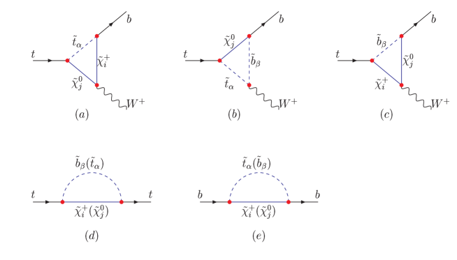
In this section we investigate the SUSY electroweak corrections. First we consider vertex corrections and quark self-energy corrections as depicted in Fig. 1. This part of the corrections are expected to be sizable for large $\tan\beta$. In Appendix A, we list in detail the relevant Feynman rules and present our analytical results. We checked that our results do reduce to those in [11] when switching off squark mixings and neglecting the $b$-quark mass in quark-squark-chargino (or neutralino) interactions.

The SUSY-EW contributions to the self-energies of gauge bosons, which are necessary to calculate for $\delta Z_{1,2}^{W}$ and $\Pi_{W}$, have been calculated by several groups [11, 20]. We recalculated them and find that our results agree with those in [11] when switching off squark mixings. In our numerical calculations we will take into account the mixings between top-squarks and between sbottoms.

As to the SUSY-EW contributions to $\Delta r$, both the universal and non-universal parts are nicely presented in [21]. We checked the analytic expressions and incorporated them in our FORTRAN code. Our numerical results show that the total contribution to the width $\Gamma(t\to Wb)$ from $\delta Z_{1,2}^{W}$, $\Pi_{W}$ and $\Delta r^{\rm SUSY-EW}$ is generally less than $1\%$.

FIG. 1.: Some of the Feynman diagrams of SUSY-EW corrections to $t\to Wb$: (a-c) are vertex loops; (d,e) are top and bottom quark self-energy loops.

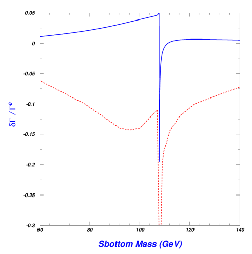
FIG. 2.: SUSY electroweak corrections to the width $\Gamma(t\to Wb)$ versus sbottom mass. The solid curve is our result and the dashed curve is taken from Fig. 7 of Ref.[13]. The input parameters are those of case C in Fig. 7 in Ref.[13].

As pointed out in Appendix A, our vertex corrections are quite different from those in [13]. To see the numerical difference between our results and those in [13], we present a comparison in Fig. 2, which corresponds to the case C of Fig. 7 in [13]. We see from Fig. 2 that the difference is significant. The results of [13] are much larger in magnitude than ours: in a large part of parameter space the results of [13] exceed $10\%$ in size while our results are below $5\%$.

Fig. 2 also shows a common feature for both results, namely, there exists a peak in the correction at $m_{\tilde{b}}\simeq 109$ GeV. This peak comes from the “threshold effect” [22], which is explained in Appendix B.

Note that some of the input parameters in Fig. 2, which were allowed at the time when the calculations in [13] were performed, may no longer be allowed nowadays. In our following numerical calculations, we will consider the current constraints on the parameters.

The relevant SUSY parameters in our calculations are: (1) $\tan\beta$, $\tilde{M}_{Q}$, $\tilde{M}_{U}$, $\tilde{M}_{D}$, $\mu$ and $A_{t,b}$ which enter the mass matrices of top-squark and sbottom [19] (see Appendix A); (2) soft-breaking gaugino masses $\tilde{M}_{1}$ and $\tilde{M}_{2}$ appearing in the chargino and neutralino mass matrices (see Appendix A); (3) the masses of sleptons and the squarks of the first two generations involved in the calculation of $\delta Z_{1,2}^{W}$, $\Pi_{W}$ and $\Delta r^{\rm SUSY-EW}$. To lessen the number of the parameters in (3), we assume an universal soft breaking parameter $\tilde{M}_{L}$ and neglect left-right mixings for sleptons and the squarks of the first two generations. Such assumptions do not affect our numerical results significantly since, as we said before, the contributions from $\delta Z_{1,2}^{W}$, $\Pi_{W}$ and $\Delta r^{\rm new}$ are small for the allowed parameter space. As for the soft breaking gaugino mass parameters $\tilde{M}_{1}$ and $\tilde{M}_{2}$, we assume the relation $\tilde{M}_{1}\simeq 0.5\tilde{M}_{2}$ [23]. With these assumptions the relevant SUSY parameters are reduced to

$$\tilde{m}_{Q},\tilde{m}_{U},\tilde{m}_{D},A_{t},A_{b},\mu,\tan{\beta},\tilde{M}_{L},\tilde{M}_{2}.$$ (16)

To estimate the size of the SUSY-EW effects, we first performed a scan over the nine parameters in Eq. (16). In our scan we restricted the parameters with mass dimensions to be less than $1$ TeV and considered the following experimental constraints:

• $\mu>0$ and a large $\tan\beta$ in the range $5\leq\tan\beta\leq 70$, which seems to be favored by the muon $g-2$ measurement [24].

• $\delta\rho<0.002$[25], which will constrain the mass splitting between stops and sbottoms. (We use the program FeynHiggs[26] to generate the values of $\delta\rho$ and the Higgs masses.)

• The LEP and CDF lower mass bounds on sparticles and the lightest CP-even Higgs boson [25, 27]

  $$m_{{\tilde{t}}}\geq 86.4~{}GeV,~{}~{}m_{{\tilde{b}}}\geq 75.0~{}GeV,~{}~{}m_{\tilde{\chi}^{+}}\geq 67.7~{}GeV,~{}~{}m_{\tilde{\chi}^{0}}\geq 40~{}GeV,$$ (17)

  $$m_{\tilde{l}}\geq 95~{}GeV,~{}~{}m_{\tilde{\nu}}\geq 41~{}GeV,~{}~{}m_{\tilde{q}}\geq 138~{}GeV,~{}~{}m_{h^{0}}\geq 91~{}GeV,$$ (18)

  where $m_{\tilde{q}}$ denotes the mass of squarks of the first two generations.

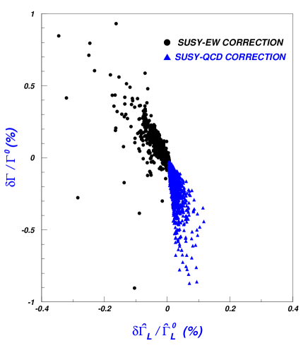
FIG. 3.: The scattered plot in the plane of $\delta\Gamma/\Gamma^{0}$ versus $\delta\hat{\Gamma}_{L}/\hat{\Gamma}_{L}^{0}$.

Our scan results are shown in Fig. 3 in the plane of $\delta\Gamma/\Gamma^{0}$ versus $\delta\hat{\Gamma}_{L}/\hat{\Gamma}_{L}^{0}$. In our calculations throughout this paper, we have fixed $G_{F}=1.16637\times 10^{-5}$ GeV^-2, $m_{W}=80.451$ GeV, $m_{t}=174.3$ GeV and $m_{b}=4.8$ GeV. Fig. 3 shows that the SUSY-EW correction is generally below one percent in size and tends to be positive for $\Gamma$ and negative for $\hat{\Gamma}_{L}$.

Although the SUSY-EW correction turns out to be quite small (below one percent in size) in the dominant part of the allowed parameter space, we found from our scan that the correction can reach a few percent in some narrow corners of the parameter space. These corners have two feathers: (1) $\mu\ll\tilde{M}_{2}$ so that the lighter chargino and the lightest neutralino are Higgsino-like, and $\tan\beta$ is large so that the $b$-quark Yukawa couplings in quark-squark-Higgsino interactions can be greatly enhanced [19]; (2) The two sparticles in a self-energy loop of top quark lie below the threshold, or in other words, the sum of the masses of the two sparticles is lighter than top quark mass. Generally speaking, for $m_{\tilde{b_{1}}}+m_{\tilde{\chi}^{+}_{1}}<m_{t}$ the sbottom($\tilde{b}_{1}$)-chargino($\tilde{\chi}^{+}_{1}$) loop can give a relatively large contribution. With the increase of $m_{\tilde{b_{1}}}$ and $m_{\tilde{\chi}^{+}_{1}}$, the contributions from this loop decrease as required by a decoupling theorem. A peak in correction size occurs at $m_{\tilde{b}_{1}}+m_{\tilde{\chi}^{+}_{1}}=m_{t}$, as shown in Fig. 2 and explained in Appendix B. To show the size of the corrections in such corners of the parameter space, we present some numerical results in two special scenarios:

• Scenario I: We assume $\mu\ll M_{2}$ and assume an universal soft-breaking mass $M_{SUSY}$ for squarks.

• Scenario II: We assume a very light sbottom $\tilde{b}_{1}$ of about $5$ GeV. So far such a light sbottom has not been ruled out by current experiments if the sbottom mixing angle $\theta_{b}$ is tuned to satisfy $\cos\theta_{b}\simeq 0.38$ [28]. For such a light sbottom, $\tan\beta$ must be large enough to cause a sufficiently large mass splitting between the two sbottom mass eigenstates. In addition, the lighter top-squark $\tilde{t}_{1}$ cannot be heavier than $300$ GeV in order to satisfy the $\delta\rho$ bound.

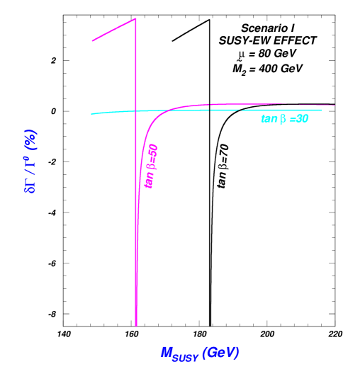
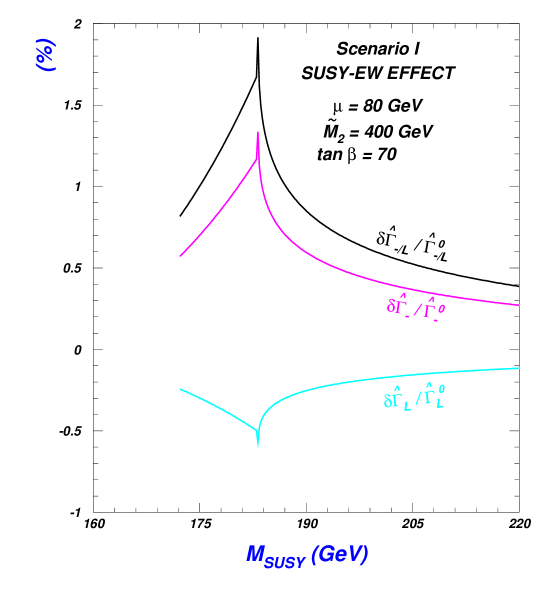
The results in Scenario I are plotted in Figs. 4 and 5. We present our result only in the region where the constraints given in the paragraph following Eq.(16) are satisfied. The peaks in these figures happen at $m_{\tilde{b}_{1}}+m_{\tilde{\chi}^{+}_{1}}=m_{t}$ where $m_{\tilde{b}_{1}}$ and $m_{\tilde{\chi}^{+}_{1}}$ are the lighter sbottom and top-squark masses, respectively. Fig. 4 shows that below the threshold the SUSY-EW corrections to the width can be as large as $3\%$ for $\tan\beta\geq 50$ and after crossing the threshold, the corrections change sharply to $-8\%$ and then quickly decrease in size. Concerning the behavior at threshold, we want to point out that the results within the region $0\leq m_{\tilde{b}}+m_{\tilde{\chi}}-m_{t}<\Gamma/2$ are not reliable since perturbative expansion of the $S$-matrix element breaks down for these points [13] (also see discussions in Appendix B). Fig. 5 shows that $\delta\hat{\Gamma}_{-}/\hat{\Gamma}_{-}^{0}$ can reach $1\%$ near the threshold and its size is generally larger than that of $\delta\hat{\Gamma}_{L}/\hat{\Gamma}_{L}^{0}$.

FIG. 4.: SUSY electroweak corrections to $\Gamma$ versus $M_{SUSY}$ in Scenario I.

FIG. 5.: SUSY eletroweak corrections to $\hat{\Gamma}_{-,L}$ and $\hat{\Gamma}_{-/L}$($\equiv\hat{\Gamma}_{-}/\hat{\Gamma}_{L}$) versus $M_{SUSY}$ in Scenario I.

Now we turn to Scenario II. For numerical calculations in Scenario II, it is inconvenient to take the parameters in Eq.(16) as input. Instead, we may choose

$$m_{\tilde{b}_{1}},m_{\tilde{t}_{1}},m_{\tilde{t}_{2}},\mu,A_{b},\theta_{b},\tan\beta,\tilde{M}_{L},\tilde{M}_{2}$$ (19)

as input parameters. Using the formula listed in Appendix A, one may relate these two sets of parameters. In our numerical calculations, we keep $\mu$ and $\tan\beta$ as variables and study the dependence on them. Other parameters are fixed to be

$$m_{\tilde{t}_{1}}=150~{}{\rm GeV},~{}~{}m_{\tilde{t}_{2}}=500~{}{\rm GeV},~{}~{}\tilde{M}_{L}=A_{b}=300~{}{\rm GeV},$$ (20)

$$m_{\tilde{b}_{1}}=5~{}{\rm GeV},~{}~{}\cos\theta_{b}=0.38,~{}~{}\tilde{M}_{2}=400~{}{\rm GeV}.$$ (21)

Note that we fixed such values for $m_{\tilde{b}_{1}}$ and $\cos\theta_{b}$ since this scenario is characterized by assuming a very light sbottom $\tilde{b}_{1}$ of about $5$ GeV with the sbottom mixing angle sytisfying $\cos\theta_{b}\simeq 0.38$ (see the definition of this scenario).

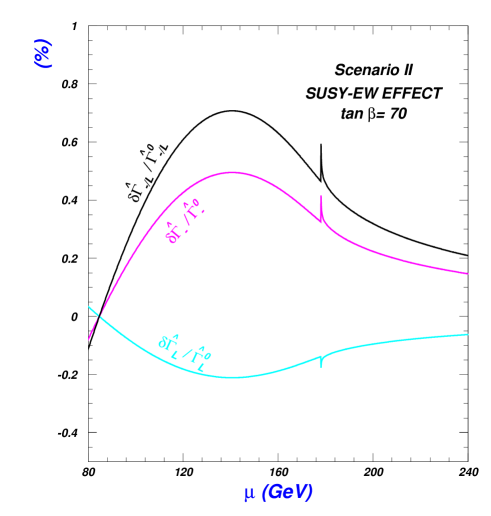
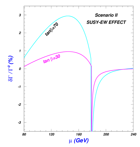
The results in Scenario II are plotted in Figs. 6 and 7. In Fig. 6 we plot $\delta\Gamma/\Gamma^{0}$ versus $\mu$ and in Fig. 7 we plot $\delta\hat{\Gamma}_{-,L}/\hat{\Gamma}_{-,L}^{0}$ and $\delta\hat{\Gamma}_{-/L}/\hat{\Gamma}_{-/L}^{0}$ versus $\mu$. Again we see that a large $\tan\beta$ can cause large SUSY-EW corrections. Fig. 6 shows a broad region of $\mu$ in which corrections to the width can be a few percent. Like in Fig. 4 the peaks occur at $m_{\tilde{b}_{1}}+m_{\tilde{\chi}}^{+}=m_{t}$. Fig.7 shows that, like in Scenario I, the SUSY-EW corrections to $\hat{\Gamma}_{-}$ and $\hat{\Gamma}_{L}$ are of opposite sign and the size of the former is larger than that of the latter.

FIG. 6.: SUSY electroweak corrections to $\Gamma$ versus $\mu$ in Scenario II.

FIG. 7.: SUSY electroweak corrections to $\hat{\Gamma}_{-,L}$ and $\hat{\Gamma}_{-/L}$ versus $\mu$ in Scenario II.

IV SUSY-QCD corrections

In this section we investigate SUSY-QCD effects. Compared with SUSY-EW corrections, SUSY-QCD corrections are easier to calculate since $\delta Z_{1,2}^{W}$, $\Pi_{W}$ and $\delta r^{\rm new}$ receive no contribution from SUSY-QCD interaction at the one-loop level and consequently, one only needs to calculate quark self-energy and vertex correction depicted in Fig. 8.

FIG. 8.: Feynman diagrams for SUSY-QCD contribution to $t\to Wb$.

Our analytical results for the form factors $F_{L,R}$ and $H_{L,R}$ agree with those in Ref.[14] and thus we do not present our analytic results here. Our numerical results for the corrections to the total width $\Gamma(t\to Wb)$ agree with Ref.[15] for the same choice of parameters.

The parameters involved in numerical evaluations are the gluino mass $m_{\tilde{g}}$, and the parameters $\tilde{m}_{Q}$, $\tilde{m}_{U}$, $\tilde{m}_{D}$, $A_{t}$, $A_{b}$, $\mu$ and $\tan{\beta}$ which enter the mass matrices of top-squark and sbottom[19]. In order to compare the size of SUSY-QCD corrections with that of SUSY-EW corrections, we have shown our scan results of SUSY-QCD corrections already in Fig. 3 in the preceding section. In our scan we have considered the relevant constraints given in the paragraph following Eq.(16) and we also required $m_{\tilde{g}}\geq 200$ GeV, which is the current experimental bound for the gluino in the framework of the minimal supergravity model[25]. From Fig. 3 one sees that the SUSY-QCD corrections and SUSY-EW corrections tend to have opposite signs and thus may cancel in large parts of parameter space. This differs drastically from the conclusion of Ref.[13, 14] which claims that the two type corrections have the same sign and thus the combined contribution can reduce the width $\Gamma(t\to Wb)$ by as much as $25\%$.

We see from Fig. 3 that in the allowed parameter space with $m_{\tilde{g}}>200$ GeV the SUSY-QCD corrections are smaller than $1\%$ in magnitude. However, we found that the corrections can reach a few percent in some corners of the parameter space if we relax the bound $m_{\tilde{g}}\geq 200$ GeV (this bound is model-dependent). In the following we present some numerical results by relaxing this bound $m_{\tilde{g}}\geq 200$ GeV, and in order to compare with SUSY-EW corrections we consider the same two scenarios as in the preceding section.

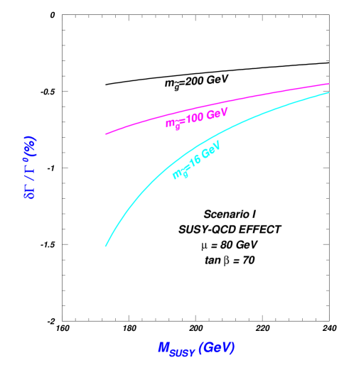
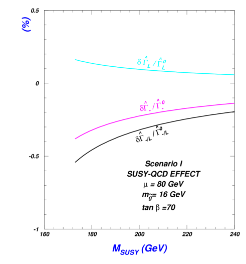
The results in Scenario I are plotted in Figs. 9 and 10 for different $m_{\tilde{g}}$ values in the allowed region of $M_{SUSY}$. We fixed $\mu=80$ GeV and $\tan\beta=70$, and included the possibility of a very light gluino of 16 GeV, which has not been excluded by current experiments (for comparison we also plot a curve with a 100 GeV gluino although it may be severely disfavored by existing experiments). Fig. 9 shows that the magnitude of SUSY-QCD corrections decrease as $M_{SUSY}$ or $m_{\tilde{g}}$ becomes large. Comparing with the SUSY-EW corrections in Fig. 4, one sees that the maximum size of the SUSY-QCD corrections is smaller than that of the SUSY-EW corrections, which can be greatly enhanced by the $b$-quark Yukawa coupling for large $\tan\beta$.

FIG. 9.: SUSY-QCD correction to $\Gamma$ versus $M_{SUSY}$ in Scenario I.

FIG. 10.: SUSY-QCD correction to $\hat{\Gamma}_{-,L}$ and $\hat{\Gamma}_{-/L}$ versus $M_{SUSY}$ in Scenario I.

Next we present results in Scenario II. Similar to the SUSY-EW case, in Scenario II it is convenient to choose

$$m_{\tilde{b}_{1}},m_{\tilde{t}_{1}},m_{\tilde{t}_{2}},\mu,A_{b},\theta_{b},\tan\beta,m_{\tilde{g}}$$ (22)

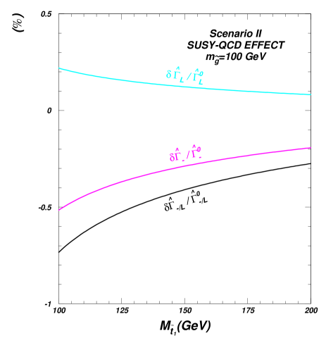
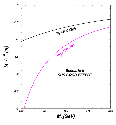
as input parameters. Our numerical studies show that the SUSY-QCD corrections are only sensitive to $m_{\tilde{t}_{1}}$ and $m_{\tilde{g}}$. So we fix $m_{\tilde{b}_{1}}=5$ GeV, $m_{\tilde{t}_{2}}=500$ GeV, $\mu=80$ GeV, $A_{b}=300$ GeV, $\tan\beta=70$ and $\cos\theta_{b}=0.38$ and plot the corrections in Figs. 11 and 12 for different gluino masses. Since in this scenario we assume a very light sbottom ($m_{\tilde{b}_{1}}=5$ GeV), we do not consider the possibility of a very light gluino ($m_{\tilde{g}}=16$ GeV) due to the $R_{b}$ constraints [30]. From the figures we see that for a $m_{\tilde{t}_{1}}=100$ GeV and $m_{\tilde{g}}=100$ GeV, SUSY-QCD corrections can reach $-3\%$, comparable in magnitude with SUSY-EW corrections.

FIG. 11.: SUSY-QCD corrections to $\Gamma$ verus the lighter top-squark mass in Scenario II.

FIG. 12.: SUSY-QCD corrections to $\hat{\Gamma}_{-,L}$ and $\hat{\Gamma}_{-/L}$ versus the lighter top-squark mass in Scenario II.

V Summary and conclusion

We investigated the one-loop SUSY-QCD and SUSY-EW corrections to the top quark decay into a $b$-quark and a longitudinal or transverse $W$-boson. The corrections are presented in terms of the longitudinal ratio $\Gamma(t\to W_{L}b)/\Gamma(t\to Wb)$ and the transverse ratio $\Gamma(t\to W_{-}b)/\Gamma(t\to Wb)$. In order to compare with the existing results in the literature, we also present the corrections to the total width $\Gamma(t\to Wb)$. To find out the typical size of these corrections, we performed a scan in the typical allowed parameter space. In order to decide if the corrections are exceptionally large in certain corners of the parameter space, we then considered some special scenarios (such as a very light sbottom or gluino). Our observations are:

• In most of the parameter space, both SUSY-QCD and SUSY-EW corrections to the ratios are less than $1\%$ in magnitude and they tend to have opposite signs. Only in some corners of the parameter space the corrections can reach a few percent.

• The corrections to the total width $\Gamma(t\to Wb)$ agree well with previous calculations for the SUSY-QCD part, but differ significantly from previous calculations for the SUSY-EW part. Unlike the previous studies, which showed a large SUSY-EW correction of more than $10\%$ in magnitude for a large part of the parameter space, our SUSY-EW results are only a few percent at most.

We conclude by remarking that these SUSY corrections, despite their smallness in size, should be taken into account in the future precision tests of the top quark decay $t\to Wb$ to determine whether SUSY is indeed the new physics chosen by Nature. (As far as we know, the corrections to the $tWb$ coupling in other kinds of new physics models are also very small [31].) However, from the viewpoint of probing SUSY through revealing its effects in the coupling $tWb$, the decay $t\to Wb$ may not be the best channel. Some single top quark production channels proceeding through the $tWb$ coupling may be complementary or even do better in this aspect. For example, SUSY effects in the $tWb$ coupling may cause observable effects in single top quark production in hadron collisions [32], and the single top quark production via electron-photon collision at a future linear collider is also quite sensitive to anomalous $tWb$ coupling [33].

A SUSY-EW loop results

In this appendix we first list the mass matrices of sfermions, charginos and neutralinos involved in our calculations, then write down the relevant interaction Lagrangian and finally present the explicit expressions of the SUSY-EW contributions from the loop diagrams shown in Fig.1.

1 Mass matrices of sfermions, charginos and neutralinos

Assuming no generation mixing for squarks in the soft-breaking terms, the mass-square matrices for up-type and down-type squarks in each generation are given respectively by [19]

$$M_{\tilde{u}}^{2} = \left(\begin{array}[]{cc}\tilde{M}_{Q}^{2}+m_{Z}^{2}\cos{2\beta}(\frac{1}{2}-e_{u}\sin^{2}{\theta_{W}})+m_{u}^{2}&m_{u}(A_{u}-\mu\cot\beta)\\ m_{u}(A_{u}-\mu\cot\beta)&\tilde{M}_{U}^{2}+m_{Z}^{2}\cos{2\beta}e_{u}\sin^{2}{\theta_{W}}+m_{u}^{2}\end{array}\right)\ ,$$ (A3)

$$M_{\tilde{d}}^{2} = \left(\begin{array}[]{cc}\tilde{M}_{Q}^{2}-m_{Z}^{2}\cos{2\beta}(\frac{1}{2}+e_{d}\sin^{2}{\theta_{W}})+m_{d}^{2}&m_{d}(A_{d}-\mu\tan\beta)\\ m_{d}(A_{d}-\mu\tan\beta)&\tilde{M}_{D}^{2}+m_{Z}^{2}\cos{2\beta}e_{d}\sin^{2}{\theta_{W}}+m_{d}^{2}\end{array}\right)\ ,$$ (A6)

where $\tilde{M}_{Q}$, $\tilde{M}_{U}$ and $\tilde{M}_{D}$ are soft-breaking mass terms for left-handed squark doublet, right-handed up and down squarks, respectively. $A_{u}$ ($A_{d}$) is the coefficient of the trilinear term $H_{2}\tilde{Q}\tilde{U}$ ($H_{1}\tilde{Q}\tilde{D}$) in soft-breaking terms, and $\tan\beta=v_{2}/v_{1}$ is the ratio of the vacuum expectation values of the two Higgs doublets.

For the first two generation squarks, the left-right mixings can be neglected due to the smallness of relevant quark masses and thus the weak-eigenstates are mass-eigenstates. From Eqs.(A3,A6), we then get the relation between the left-handed up-type squark mass $M_{\tilde{u}_{L}}$ and the left-handed down-type squark mass $M_{\tilde{d}_{L}}$

$$M_{\tilde{u}_{L}}^{2}=M_{\tilde{d}_{L}}^{2}+m_{Z}^{2}\cos{2\beta}(1-\sin^{2}\theta_{W})+m_{u}^{2}-m_{d}^{2}\ .$$ (A7)

For the third generation squarks, the left-right mixings cannot be neglected and the mass-eigenstates $\tilde{q}_{1,2}$ ($q=t,b$) are related to the weak-eigenstates $\tilde{q}_{L,R}$ by an unitary rotation $R$

$$\left(\begin{array}[]{l}\tilde{q}_{1}\\ \tilde{q}_{2}\end{array}\right)=R\left(\begin{array}[]{l}\tilde{q}_{L}\\ \tilde{q}_{R}\end{array}\right)\equiv\left(\begin{array}[]{cc}\cos\theta_{q}&\sin\theta_{q}\\ -\sin\theta_{q}&\cos\theta_{q}\end{array}\right)\left(\begin{array}[]{l}\tilde{q}_{L}\\ \tilde{q}_{R}\end{array}\right)\ ,$$ (A16)

where $\theta_{q}$ is the so-called mixing angle between $\tilde{q}_{L}$ and $\tilde{q}_{R}$.

The mass-square matrices in Eqs.(A3, A6) can be alternatively expressed by the squark masses and mixing angle as

$$M^{2}_{\tilde{q}}=\left(\begin{array}[]{cc}\cos^{2}\theta_{q}m_{\tilde{q}_{1}}^{2}+\sin^{2}\theta_{q}m_{\tilde{q}_{2}}^{2}&\sin\theta_{q}\cos\theta_{q}(m_{\tilde{q}_{1}}^{2}-m_{\tilde{q}_{2}}^{2})\\ \sin\theta_{q}\cos\theta_{q}(m_{\tilde{q}_{1}}^{2}-m_{\tilde{q}_{2}}^{2})&\sin^{2}\theta_{q}m_{\tilde{q}_{1}}^{2}+\cos^{2}\theta_{q}m_{\tilde{q}_{2}}^{2}\end{array}\right)\ .$$ (A19)

By comparing Eq.(A19) with Eqs.(A3, A6), one can obtain the relationship between the two set of input parameters in the squark sector, ($m_{\tilde{q}_{1}}$, $m_{\tilde{q}_{2}}$, $\theta_{q}$) and ($\tilde{M}_{Q}$, $\tilde{M}_{U}$, $\tilde{M}_{D}$, $A_{t,b}$, $\mu$). The mass matrices for sleptons take the similar forms as for squarks. But due to the smallness of lepton masses, the left-right mixings can be neglected for the three generations.

The mass matrices of charginos and neutralinos are also involved in our calculations. The chargino mass matrix can be diagonalized by two unitary matrices $U$ and $V$

$$U^{\ast}\left(\begin{array}[]{cc}\tilde{M}_{2}&m_{W}\sqrt{2}\sin\beta\\ m_{W}\sqrt{2}\cos{\beta}&\mu\end{array}\right)V^{-1}={\rm diag}\left\{m_{\tilde{\chi}^{+}_{i}}\right\}\ \ \ \ (i=1,2)\ .$$ (A22)

The neutralino mass matrix is given by

$$Y=\left(\begin{array}[]{cccc}\tilde{M}_{1}&0&-m_{Z}\sin\theta_{W}\cos\beta&m_{Z}\sin\theta_{W}\sin\beta\\ 0&\tilde{M}_{2}&m_{Z}\cos\theta_{W}\cos\beta&-m_{Z}\cos\theta_{W}\sin\beta\\ -m_{Z}\sin\theta_{W}\cos\beta&m_{Z}\cos\theta_{W}\cos\beta&0&-\mu\\ m_{Z}\sin\theta_{W}\sin\beta&-m_{Z}\cos\theta_{W}\sin\beta&-\mu&0\end{array}\right)\ ,$$ (A27)

and it can be diagonalized by an unitary matrix $N$

$$N^{\ast}YN^{-1}={\rm diag}\left\{m_{\tilde{\chi}^{0}_{j}}\right\}\ \ \ \ (j=1,2,3,4)\ .$$ (A28)

In the above expressions $\tilde{M}_{1}$ and $\tilde{M}_{2}$ are respectively the soft-breaking $U(1)$ and $SU(2)$ gaugino masses. $m_{\tilde{\chi}^{+}_{i}}$ and $m_{\tilde{\chi}^{0}_{j}}$ are the masses of charginos and neutralinos, respectively. One point we want to mention is that $U$, $V$ and $N$ defined in Eq.(A22, A28) are not unique and one should choose $U$, $V$ and $N$ in a way that all the masses of charginos and neutralinos are positive.

2 Interaction Lagrangian

The interaction Lagrangian relevant for our calculations is given by

$${\cal L} = -\frac{g}{2}\left\{\tilde{t}^{\ast}_{\alpha}\bar{\tilde{\chi}}^{-}_{i}(A_{\alpha i}^{t}-B_{\alpha i}^{t}\gamma_{5})b+\tilde{b}^{\ast}_{\beta}\bar{\tilde{\chi}}^{+}_{i}(A_{\beta i}^{b}-B_{\beta i}^{b}\gamma_{5})t+\tilde{t}^{\ast}_{\alpha}\bar{\tilde{\chi}}^{0}_{j}(A_{\alpha j}^{t(0)}-B_{\alpha j}^{t(0)}\gamma_{5})t+\tilde{b}^{\ast}_{\beta}\bar{\tilde{\chi}}^{0}_{j}(A_{\beta j}^{b(0)}-B_{\beta j}^{b(0)}\gamma_{5})b\right\}$$ (A31)

$$-\frac{g}{\sqrt{2}}R_{\alpha 1}^{t}R_{\beta 1}^{b}\tilde{t}^{\ast}_{\alpha}\stackrel{{\scriptstyle\leftrightarrow}}{{\partial^{\mu}}}\tilde{b}_{\beta}W_{\mu}^{+}+g\bar{\tilde{\chi}}^{0}_{j}\gamma^{\mu}(O_{ij}^{L}P_{L}+O_{ij}^{R}P_{R})\tilde{\chi}^{-}_{i}W_{\mu}^{+}$$

$$+\frac{g^{2}}{2}(R^{t}_{\alpha_{1}1}R^{t}_{\alpha_{2}1}\tilde{t}^{\ast}_{\alpha_{1}}\tilde{t}_{\alpha_{2}}+R^{b}_{\beta_{1}1}R^{b}_{\beta_{2}1}\tilde{b}^{\ast}_{\beta_{1}}\tilde{b}_{\beta_{2}})W_{\mu}^{-}W^{\mu+}+h.c.\ ,$$

where the sum over repeated indices is implied, and

$$A^{t}_{\alpha i} = R^{t}_{\alpha 1}(V^{\ast}_{i1}-\lambda_{b}U_{i2})-R^{t}_{\alpha 2}\lambda_{t}V_{i2}^{\ast}\ ,$$ (A32)

$$B^{t}_{\alpha i} = R^{t}_{\alpha 1}(V^{\ast}_{i1}+\lambda_{b}U_{i2})-R^{t}_{\alpha 2}\lambda_{t}V_{i2}^{\ast}\ ,$$ (A33)

$$A^{b}_{\beta i} = R^{b}_{\beta 1}(U^{\ast}_{i1}-\lambda_{t}V_{i2})-R^{b}_{\beta 2}\lambda_{b}U_{i2}^{\ast}\ ,$$ (A34)

$$B^{b}_{\beta i} = R^{b}_{\beta 1}(U^{\ast}_{i1}+\lambda_{t}V_{i2})-R^{b}_{\beta 2}\lambda_{b}U_{i2}^{\ast}\ ,$$ (A35)

$$A^{t(0)}_{\alpha j} = R^{t}_{\alpha 1}(\lambda_{t}N_{j4}+\sqrt{2}(\frac{1}{6}N_{j1}^{\ast}\tan\theta_{W}+\frac{1}{2}N_{j2}^{\ast}))+R^{t}_{\alpha 2}(\lambda_{t}N_{j4}^{\ast}-\sqrt{2}\frac{2}{3}N_{j1}\tan\theta_{W})\ ,$$ (A36)

$$B^{t(0)}_{\alpha j} = R^{t}_{\alpha 1}(-\lambda_{t}N_{j4}+\sqrt{2}(\frac{1}{6}N_{j1}^{\ast}\tan\theta_{W}+\frac{1}{2}N_{j2}^{\ast}))+R^{t}_{\alpha 2}(\lambda_{t}N_{j4}^{\ast}+\sqrt{2}\frac{2}{3}N_{j1}\tan\theta_{W})\ ,$$ (A37)

$$A^{b(0)}_{\beta j} = R^{b}_{\beta 1}(\lambda_{b}N_{j3}+\sqrt{2}(\frac{1}{6}N_{j1}^{\ast}\tan\theta_{W}-\frac{1}{2}N_{j2}^{\ast}))+R^{b}_{\beta 2}(\lambda_{b}N_{j3}^{\ast}+\frac{\sqrt{2}}{3}N_{j1}\tan\theta_{W})\ ,$$ (A38)

$$B^{b(0)}_{\beta j} = R^{b}_{\beta 1}(-\lambda_{b}N_{j3}+\sqrt{2}(\frac{1}{6}N_{j1}^{\ast}\tan\theta_{W}-\frac{1}{2}N_{j2}^{\ast}))+R^{b}_{\beta 2}(\lambda_{b}N_{j3}^{\ast}-\frac{\sqrt{2}}{3}N_{j1}\tan\theta_{W})\ ,$$ (A39)

$$O_{ij}^{L} = -\frac{1}{\sqrt{2}}N_{j4}V_{i2}^{\ast}+N_{j2}V_{i1}^{\ast}\ ,$$ (A40)

$$O_{ij}^{R} = \frac{1}{\sqrt{2}}N_{j3}^{\ast}U_{i2}+N_{j2}^{\ast}U_{i1}\ .$$ (A41)

Here $\lambda_{t}=\frac{m_{t}}{\sqrt{2}m_{W}\sin\beta}$ and $\lambda_{b}=\frac{m_{b}}{\sqrt{2}m_{W}\cos\beta}$. As for the notations for chargino and neutralino mass matrices, we follow the notations of Ref.[19] rather than those of Ref.[13]. Note, however, that the resulting interactions are the same.

3 Analytic results of SUSY-EW loops

To compare our results with those in Ref. [13], we present our results in the same way as in Ref.[13]. First, from matrices in Eqs.(A32-A41) we define the following matrices

$$A_{\pm}^{t}=A^{t}\pm B^{t}\ ,\ \ \ \ A_{\pm}^{t(0)}=A^{t(0)}\pm B^{t(0)}\ ,$$ (A42)

$$A_{\pm}^{b}=A^{b}\pm B^{b}\ ,\ \ \ \ A_{\pm}^{b(0)}=A^{b(0)}\pm B^{b(0)}\ ,$$ (A43)

and construct the combinations as

$$A^{(1)} = -A_{+}^{t\ast}O^{R}A_{-}^{t(0)}\ ,\ \ \ \ E^{(1)}=-A_{-}^{t\ast}O^{R}A_{-}^{t(0)}\ ,$$ (A44)

$$B^{(1)} = -A_{+}^{t\ast}O^{R}A_{+}^{t(0)}\ ,\ \ \ \ F^{(1)}=-A_{-}^{t\ast}O^{R}A_{+}^{t(0)}\ ,$$ (A45)

$$C^{(1)} = -A_{+}^{t\ast}O^{L}A_{-}^{t(0)}\ ,\ \ \ \ G^{(1)}=-A_{-}^{t\ast}O^{L}A_{-}^{t(0)}\ ,$$ (A46)

$$D^{(1)} = -A_{+}^{t\ast}O^{L}A_{+}^{t(0)}\ ,\ \ \ \ H^{(1)}=-A_{-}^{t\ast}O^{L}A_{+}^{t(0)}\ ,$$ (A47)

$$A^{(2)} = -R_{\alpha 1}^{t}R_{\beta 1}^{b}A_{+}^{b(0)\ast}A_{-}^{t(0)}\ ,\ \ \ \ C^{(2)}=-R_{\alpha 1}^{t}R_{\beta 1}^{b}A_{-}^{b(0)\ast}A_{-}^{t(0)}\ ,$$ (A48)

$$B^{(2)} = -R_{\alpha 1}^{t}R_{\beta 1}^{b}A_{+}^{b(0)\ast}A_{+}^{t(0)}\ ,\ \ \ \ D^{(2)}=-R_{\alpha 1}^{t}R_{\beta 1}^{b}A_{-}^{b(0)\ast}A_{+}^{t(0)}\ ,$$ (A49)

$$A^{(3)} = A_{+}^{b(0)\ast}O^{L}A_{-}^{b}\ ,\ \ \ \ E^{(3)}=A_{-}^{b(0)\ast}O^{L}A_{-}^{b}\ ,$$ (A50)

$$B^{(3)} = A_{+}^{b(0)\ast}O^{L}A_{+}^{b}\ ,\ \ \ \ F^{(3)}=A_{-}^{b(0)\ast}O^{L}A_{+}^{b}\ ,$$ (A51)

$$C^{(3)} = A_{+}^{b(0)\ast}O^{R}A_{-}^{b}\ ,\ \ \ \ G^{(3)}=A_{-}^{b(0)\ast}O^{R}A_{-}^{b}\ ,$$ (A52)

$$D^{(3)} = A_{+}^{b(0)\ast}O^{R}A_{+}^{b}\ ,\ \ \ \ H^{(3)}=A_{-}^{b(0)\ast}O^{R}A_{+}^{b}\ .$$ (A53)

Then the contributions of vertex loop diagrams (a,b,c) in Fig.1 to the form factors $F_{L,R}$ and $H_{L,R}$ are given as follows.

• Diagram (a):

  $$F_{L}^{(a)} = \frac{\sqrt{2}g^{2}}{4V_{tb}}\frac{1}{16\pi^{2}}\left\{-\frac{1}{2}D^{(1)}(-1+4C_{24})+m_{\tilde{\chi}^{0}_{j}}m_{\tilde{\chi}^{-}_{i}}B^{(1)}C_{0}-m_{\tilde{\chi}^{0}_{j}}m_{t}C^{(1)}(C_{11}-C_{12})\right.$$ (A55)

  $$\left.+m_{\tilde{\chi}^{-}_{i}}m_{t}A^{(1)}(C_{0}+C_{11}-C_{12})-m_{t}^{2}D^{(1)}(C_{11}-C_{12}+C_{21}-C_{23})-m_{W}^{2}D^{(1)}(C_{22}-C_{23})\right\}\ ,$$

  $$F_{R}^{(a)} = \frac{\sqrt{2}g^{2}}{4V_{tb}}\frac{1}{16\pi^{2}}\left\{-\frac{1}{2}E^{(1)}(-1+4C_{24})+m_{\tilde{\chi}^{0}_{j}}m_{\tilde{\chi}^{-}_{i}}G^{(1)}C_{0}-m_{\tilde{\chi}^{0}_{j}}m_{t}F^{(1)}(C_{11}-C_{12})\right.$$ (A57)

  $$\left.+m_{\tilde{\chi}^{-}_{i}}m_{t}H^{(1)}(C_{0}+C_{11}-C_{12})-m_{t}^{2}E^{(1)}(C_{11}-C_{12}+C_{21}-C_{23})-m_{W}^{2}E^{(1)}(C_{22}-C_{23})\right\}\ ,$$

  $$H_{L}^{(a)} = \frac{\sqrt{2}g^{2}}{4V_{tb}}\frac{1}{16\pi^{2}}\left\{2m_{\tilde{\chi}^{0}_{j}}F^{(1)}(C_{11}-C_{12})+2m_{\tilde{\chi}^{-}_{i}}H^{(1)}C_{12}+2m_{t}E^{(1)}(C_{11}-C_{12}+C_{21}-C_{23})\right\}\ ,$$ (A58)

  $$H_{R}^{(a)} = \frac{\sqrt{2}g^{2}}{4V_{tb}}\frac{1}{16\pi^{2}}\left\{2m_{\tilde{\chi}^{0}_{j}}C^{(1)}(C_{11}-C_{12})+2m_{\tilde{\chi}^{-}_{i}}A^{(1)}C_{12}+2m_{t}D^{(1)}(C_{11}-C_{12}+C_{21}-C_{23})\right\}\ ,$$ (A59)

  where the functions $C_{0}$ and $C_{nm}$ are 3-point Feynman integrals defined in Ref. [34] with functional dependence $C_{0},C_{nm}(-p_{t},p_{W},m_{\tilde{t}_{\alpha}},m_{\tilde{\chi}_{j}^{0}},m_{\tilde{\chi}_{i}^{-}})$.

• Diagram (b):

  $$F_{L}^{(b)} = \frac{g^{2}}{2V_{tb}}\frac{1}{16\pi^{2}}\left\{-B^{(2)}C_{24}\right\}\ ,$$ (A60)

  $$F_{R}^{(b)} = \frac{g^{2}}{2V_{tb}}\frac{1}{16\pi^{2}}\left\{-C^{(2)}C_{24}\right\}\ ,$$ (A61)

  $$H_{L}^{(b)} = \frac{g^{2}}{2V_{tb}}\frac{1}{16\pi^{2}}\left\{m_{\tilde{\chi}^{0}_{j}}D^{(2)}(C_{0}+C_{11})+m_{t}C^{(2)}(C_{12}-C_{11}-C_{21}+C_{23})\right\}\ ,$$ (A62)

  $$H_{R}^{(a)} = \frac{g^{2}}{2V_{tb}}\frac{1}{16\pi^{2}}\left\{m_{\tilde{\chi}^{0}_{j}}A^{(2)}(C_{0}+C_{11})+m_{t}B^{(2)}(C_{12}-C_{11}-C_{21}+C_{23})\right\}\ ,$$ (A63)

  with the Feynman integrals $C_{0},C_{nm}(-p_{t},p_{W},m_{\tilde{\chi}^{0}_{j}},m_{\tilde{t}_{\alpha}},m_{\tilde{b}_{\beta}})$.

• Diagram (c) :

  $F_{L,R}^{(c)}$ and $H_{L,R}^{(c)}$ can be obtained from the corresponding $F_{L,R}^{(a)}$ and $H_{L,R}^{(a)}$ with the replacements:

  $$m_{\tilde{t}_{\alpha}}\to m_{\tilde{b}_{\beta}}\ ,\ \ \ \ \ \ m_{\tilde{\chi}_{j}^{0}}\leftrightarrow m_{\tilde{\chi}_{i}^{-}}\ ,\ \ \ \ \ \ A^{(1)}\to A^{(3)}\ ,\ \ \ \ \ \ B^{(1)}\to B^{(3)}\ ,$$ (A64)

  $$C^{(1)}\to C^{(3)}\ ,\ \ \ \ \ \ D^{(1)}\to D^{(3)}\ ,\ \ \ \ \ \ E^{(1)}\to E^{(3)}\ ,\ \ \ \ \ \ H^{(1)}\to H^{(3)}\ .$$ (A65)

For the self-energy loop diagrams in (d,e) of Fig. 1, we only present the corresponding forms of $\Sigma_{\tilde{\chi}^{-}}$ (from chargino loops) and of $\Sigma_{\tilde{\chi}^{0}}$ (from neutralino loops). The renormalization constants $\delta Z_{t,b}^{L}$ can be obtained in a straitforward manner by using Eqs.(10, 11). The results are given by

• Diagram (d) :

  $$\Sigma_{\tilde{\chi}^{-}}^{t}(p) = \frac{g^{2}}{4}\frac{1}{16\pi^{2}}\left\{(|A^{b}_{+}|^{2}\not{\hbox{\kern-2.1pt$p$}}P_{L}+|A^{b}_{-}|^{2}\not{\hbox{\kern-2.1pt$p$}}P_{R})B_{1}(p,m_{\tilde{\chi}_{i}^{-}},m_{\tilde{b}_{\beta}})\right.$$ (A67)

  $$\left.-m_{\tilde{\chi}_{i}^{-}}(A_{-}^{b\ast}A_{+}^{b}P_{L}+A_{+}^{b\ast}A_{-}^{b}P_{R})B_{0}(p,m_{\tilde{\chi}_{i}^{-}},m_{\tilde{b}_{\beta}})\right\}\ ,$$

  $$\Sigma_{\tilde{\chi}^{0}}^{t}(p) = \frac{g^{2}}{4}\frac{1}{16\pi^{2}}\left\{(|A^{t(0)}_{+}|^{2}\not{\hbox{\kern-2.1pt$p$}}P_{L}+|A^{t(0)}_{-}|^{2}\not{\hbox{\kern-2.1pt$p$}}P_{R})B_{1}(p,m_{\tilde{\chi}_{j}^{0}},m_{\tilde{t}_{\alpha}})\right.$$ (A69)

  $$\left.-m_{\tilde{\chi}_{j}^{0}}(A_{-}^{t(0)\ast}A_{+}^{t(0)}P_{L}+A_{+}^{t(0)\ast}A_{-}^{t(0)}P_{R})B_{0}(p,m_{\tilde{\chi}_{j}^{0}},m_{\tilde{t}_{\alpha}})\right\}\ .$$

• Diagram (e) :

  $$\Sigma_{\tilde{\chi}^{-}}^{b}(p) = \frac{g^{2}}{4}\frac{1}{16\pi^{2}}\left\{(|A^{t}_{+}|^{2}\not{\hbox{\kern-2.1pt$p$}}P_{L}+|A^{t}_{-}|^{2}\not{\hbox{\kern-2.1pt$p$}}P_{R})B_{1}(p,m_{\tilde{\chi}_{i}^{-}},m_{\tilde{t}_{\alpha}})\right.$$ (A71)

  $$\left.-m_{\tilde{\chi}_{i}^{-}}(A_{-}^{t\ast}A_{+}^{t}P_{L}+A_{+}^{t\ast}A_{-}^{t}P_{R})B_{0}(p,m_{\tilde{\chi}_{i}^{-}},m_{\tilde{t}_{\alpha}})\right\}\ ,$$

  $$\Sigma_{\tilde{\chi}^{0}}^{b}(p) = \frac{g^{2}}{4}\frac{1}{16\pi^{2}}\left\{(|A^{b(0)}_{+}|^{2}\not{\hbox{\kern-2.1pt$p$}}P_{L}+|A^{b(0)}_{-}|^{2}\not{\hbox{\kern-2.1pt$p$}}P_{R})B_{1}(p,m_{\tilde{\chi}_{j}^{0}},m_{\tilde{b}_{\beta}})\right.$$ (A73)

  $$\left.-m_{\tilde{\chi}_{j}^{0}}(A_{-}^{b(0)\ast}A_{+}^{b(0)}P_{L}+A_{+}^{b(0)\ast}A_{-}^{b(0)}P_{R})B_{0}(p,m_{\tilde{\chi}_{j}^{0}},m_{\tilde{b}_{\beta}})\right\}\ .$$

Comparing our results with those in [13], we found that our self-energy loop results essentially agree with those of [13], but our vertex loop results disagree with those of [13]. The analytic results of [13] seem to have some explicit errors, e.g., it seems to be impossible to cancel the UV divergence in $F_{L}$, terms like $m_{t}C_{0}$ should not appear in $H_{L,R}$ and $G_{2}$ and $G_{3}$ should be interchanged.

B Explanation of threshold behaviors

The two-point loop functions $B_{0,1}^{\prime}(p,m_{1},m_{2})|_{p^{2}=m_{t}^{2}}$ enter our results via $\delta Z_{t}^{L}$. In order to explain the threshold behavior in Figs.(2, 4, 6), we study the behavior of $B_{0,1}^{\prime}(m_{0},m_{1},m_{2})$ near the threshold point $m_{0}=m_{1}+m_{2}$. We take $B_{0}^{\prime}$ as an example, the behavior of $B_{1}^{\prime}$ is similar.

For fixed $m_{0}$ and $m_{2}$, $B_{0}^{\prime}(m_{0},m_{1},m_{2})$ as a function of $m_{1}$ can be expressed as

$$B_{0}^{\prime} = \int_{0}^{1}\frac{x-x^{2}}{m_{0}^{2}x^{2}-(m_{0}^{2}+m_{1}^{2}-m_{2}^{2})x+m_{1}^{2}}dx$$ (B1)

$$= \left\{\begin{array}[]{lll}\frac{1}{m_{0}^{2}}\int_{0}^{1}\frac{x-x^{2}}{(x-a)^{2}-b^{2}}dx&{\rm for}&\ \ m_{1}<m_{0}-m_{2}\ ,\\ \frac{1}{m_{0}^{2}}\int_{0}^{1}\frac{x-x^{2}}{(x-a)^{2}}dx&{\rm for}&\ \ m_{1}=m_{0}-m_{2}\ ,\\ \frac{1}{m_{0}^{2}}\int_{0}^{1}\frac{x-x^{2}}{(x-a)^{2}+b^{2}}dx&{\rm for}&\ \ m_{1}>m_{0}-m_{2}\ ,\end{array}\right.$$ (B5)

where

$$a = \frac{m_{0}^{2}+m_{1}^{2}-m_{2}^{2}}{2m_{0}^{2}}\ ,$$ (B6)

$$b = \frac{1}{2m_{0}^{2}}\sqrt{|(m_{0}+m_{1}+m_{2})(m_{0}+m_{1}-m_{2})(m_{0}-m_{1}+m_{2})(m_{0}-m_{1}-m_{2})|}\ .$$ (B7)

From Eq.(B5), one may infer that, in regions below threshold ($m_{1}<m_{0}-m_{2}$) or above threshold ($m_{1}>m_{0}-m_{2}$), $B_{0}^{\prime}$ is an continuous function of $m_{1}$. At the threshold point ($m_{1}=m_{0}-m_{2}$), $B_{0}^{\prime}$ is divergent due to the fact $0<a<1$. (In some calculation programs, such as LoopTools [35] used in our calculations, an imaginary part is added to the propagators in the loops to avoid the divergence at the threshold point.)

In the limit $m_{1}\to m_{0}-m_{2}$ from the lower (i.e. $m_{1}<m_{0}-m_{2}$), one has $B_{0}^{\prime}\to-2+(1-2a)\ln\left[(1-a)/a\right]$ which is a finite value and corresponds to the top points in Figs.(2, 4, 6). But in the limit $m_{1}\to m_{0}-m_{2}$ from the upper (i.e. $m_{1}>m_{0}-m_{2}$), one has $B_{0}^{\prime}\to\infty$ which corresponds to the bottom point in Figs.(2, 4, 6). Since these bottom points tend to take very large negative values, the perturbative calculation is not reliable at these points and a special treatment is needed [36].

REFERENCES

• [1] For example, top-pair production at hadron collisions are quite sensitive to new physics. For comprehensive model-independent analyses, see, e.g., C. T. Hill and S. J. Parke, Phys. Rev. D 49, 4454 (1994); K. Whisnant, et al., Phys. Rev. D 56, 467 (1997); K. Hikasa, et al., Phys. Rev. D 58, 114003 (1998).
• [2] For recent reviews on top quark, see, e.g., C. T. Hill and E. Simmons, hep-ph/0203079; C.-P. Yuan, hep-ph/0203088; E. Simmons, hep-ph/0211335; S. Willenbrock, hep-ph/0211067; D. Chakraborty, J. Konigsberg, D. Rainwater, hep-ph/0303092.
• [3] See, e.g., A. Datta, et al., Phys. Rev. D 56, 3107 (1997); R. J. Oakes, et al., Phys. Rev. D 57, 534 (1998); K. Hikasa, J. M. Yang, B.-L. Young, Phys. Rev. D 60, 114041 (1999); C. Balazs, H.-J. He, C.-P. Yuan, Phys. Rev. D 60, 114001 (1999); H.-J. He, C.P. Yuan, Phys. Rev. Lett. 83, 28 (1999); G. Burdman, Phys. Rev. Lett. 83, 2888 (1999); P. Chiappetta, et al., Phys. Rev. D 61, 115008 (2000); J. Cao, Z. Xiong and J. M. Yang, Nucl. Phys. B 651, 87 (2003); Phys. Rev. D 67, 071701 (2003).
• [4] See, e.g., M. Hosch, et al., Phys. Rev. D 58, 034002 (1998); S. Mrenna and C.P. Yuan, Phys. Lett. B 367, 188 (1996). C. S. Li, R. J. Oakes and J. M. Yang, Phys. Rev. D 49, 293 (1994); J. L. Lopez, D. V. Nanopoulos and R. Rangarajan, Phys. Rev. D 56, 3100 (1997); G. Eilam, et al., Phys. Lett. B 510, 227 (2001); K.J. Abraham, et al., Phys. Lett. B 514, 72 (2001); Phys. Rev. D 63, 034011 (2001); T. Han and J. Hewett, Phys. Rev. D 60, 074015 (1999); F. del Aguila, J. A. Aguilar-Saavedra, R. Miquel, Phys. Rev. Lett. 82, 1628 (1999); X. L. Wang et al., Phys. Rev. D 50, 5781 (1994).
• [5] See, e.g., C. A. Nelson, et. al., Phys. Rev. D 56, 5928(1997); Phys. Rev. D 57, 5923 (1998); C. A. Nelson and A. M. Cohen, Eur. Phys. J. C 8, 393 (1999); C. A. Nelson and L. J. Adler, Eur. Phys. J. C 17, 399 (2000); C. A. Nelson, Eur. Phys. J. C 19, 323 (2001); F. del Aguila and J. A. Aguilar-Saavedra, Phys. Rev. D 67, 014009 (2003).
• [6] Y. Bigi, et. al., Phys. Lett. B 181, 157 (1986).
• [7] CDF collaboration, T. Affolder, et al., Phys. Rev. Lett. 84, 216 (2000).
• [8] S. Willenbrock , Rev. Mod. Phys. 72, 1141(2000).
• [9] M. Fischer, S. Groote, J. G. Körner and M. C. Mauser, Phys. Lett. B 451, 406 (1999); Phys. Rev. D 63, 031501 (2001); Phys. Rev. D 65, 054036 (2002).
• [10] M. Fischer, S. Groote, J. G. Körner and M. C. Mauser, Phys. Rev. D 67, 091501 (2003).
• [11] J. M. Yang and C. S. Li, Phys. Lett. B 320, 117 (1994).
• [12] C. S. Li, J. M. Yang and B. Q. Hu, Phys. Rev. D 48, 5425 (1993).
• [13] D. Garcia, R. A. Jiménez, J. Solá and W. Hollik, Nucl. Phys. B 427, 53 (1994).
• [14] A. Dabelstein, W. Hollik, C. Jünger, R. A.  Jiménez and J. Solá, Nucl. Phys. B 454, 75 (1995).
• [15] A. Brandenburg and M. Maniatis, Phys. Lett. B 545, 139 (2002).
• [16] B. Grzadkowski and W. Hollik, Nucl. Phys. B 384, 101 (1992).
• [17] M. Bohm, H. Spiesberger and W. Hollik, Fortsch. Phys. 34, 687 (1986); W. Hollik, Fortsch. Phys. 38, 165(1990).
• [18] A. Denner, Fortsch. Phys. 41, 307 (1993).
• [19] H. E. Haber and G. L. Kane, Phys. Rept. 117, 75 (1985); J. F. Gunion and H. E. Haber, Nucl. Phys. B 272, 1 (1986).
• [20] See, e.g., J. A. Grifols and J. Solá, Nucl. Phys. B 253, 47 (1985); D. Garcia and J. Solá, Mod. Phys. Lett. A 9, 211 (1994); R. Hempfling and B. A. Kniehl, Z. Phys. C 59, 263 (1993).
• [21] P. H. Chankowski, et.al., Nucl. Phys. B 417, 101 (1994).
• [22] J. Fleischer and F. Jegerlehner, Phys. Rev. D 23, 2001 (1981); Nucl. Phys. B 216, 469 (1983); A. Dabelstein and W. Hollik, Z. Phys. C 53, 507 (1992).
• [23] H. P. Nilles, Phys. Rept. 110, 1 (1984); A. B. Lahanas and D. V. Nanopoulos, Phys. Rept.  145, 1 (1987).
• [24] H. N Brown, et al., Mu g-2 Collaboration, Phys. Rev. Lett. 86, 2227 (2001).
• [25] Particle Physics Group. Eur. Phys. J. C 15, 274 (2000).
• [26] S. Heinemeyer, W. Hollik and G. Weiglein, Comput. Phys. Commun. 124, 76 (2000).
• [27] R. Barate et al., ALEPH Collaboration, Phys. Lett. B 499, 53 (2001); LEP Higgs Working Group, hep-ex/0107029; hep-ex/0107030; U. Schwickerath, hep-ph/0205126.
• [28] M. Carena, S. Heinemeyer, C. E. Wagner and G. Weiglein, Phys. Rev. Lett. 86, 4463 (2001).
• [29] E. L. Berger, et. al., Phys. Rev. Lett. 86, 4231 (2001).
• [30] J. Cao, Z. Xiong and J. M. Yang, Phys. Rev. Lett. 88, 111802 (2002); G. C. Cho, Phys. Rev. Lett. 89, 091801 (2002); K. Cheung and W. Y. Keung, Phys. Rev. Lett. 89, 221801 (2002); Z. Luo and J. L. Rosner, hep-ph/0306022; R. Malhotra, hep-ph/0306183.
• [31] See, e.g., N. Mahajan, hep-ph/0304235.
• [32] C. S. Li, et al., Phys. Rev. D 57,2009 (1998); Phys. Lett. B 98, 298 (1997); Phys. Rev. D 55, 5780 (1997);
• [33] J. J. Cao et al., Phys. Rev. D 58, 094004 (1998); E. Boos, et al., Eur. Phys. J. C 21, 81 (2001).
• [34] A. Axelrod, Nucl. Phys. B 209, 349 (1982).
• [35] T. Hahn, Nucl. Phys. Proc. Suppl.89, 231 (2000); Acta Phys. Plon. B30, 3469 (1999).
• [36] T. Bhattacharya and S. Willenbrock, Phys. Rev. D 47, 4022 (1993); B. A. Kniehl, C. P. Palisoc and A. Sirlin, Nucl. Phys. B 591, 296 (2000).