Abstract

We investigate the possibility to disentangle the radions in the Randall-Sundrum scenario from higgs boson at the next generation high energy $e^{+}e^{-}$ linear colliders. Due to trace anomaly, the radion coupling (and in turn the branching ratio) to gluons is enhanced over the same for the Standard Model (SM) higgs. We study the radion $\phi$ production at electron-positron colliders, via the process $e^{+}e^{-}\rightarrow\nu\bar{\nu}\phi$, and propose to investigate radion decay to a pair of gluons. At 500 GeV center of mass energy, our signal is not very promising. We find our results are encouraging for finding radion and differentiating it from higgs for center of mass energies of 1 TeV and above.

Recently proposed models [1, 2], aiming to cure the hierarchy problem between electroweak (EW) and Planck scale, offer an exciting possibility to test the gravitational interactions at the TeV colliders. The models in [1, 2] require our universe to have $(3+n)+1$ space-time dimensions, of which the extra, $n$, space-like dimensions are compactified. The ADD [1] model requires relatively large compactification radius ($\sim 1~{}mm$). In the Randall-Sundrum (RS) scenario [2], which is the focus of this analysis, there is only one extra space-like dimension compactified on an $S_{1}/Z_{2}$ orbifold. Unlike the ADD, RS-scenario does not require a large compactification radius for the extra compactified space-like dimension. The radius of compactification is of the order of the Planck length, and interestingly it is a dynamical object. Moreover, the assumed geometry of space-time is non-factorisable in the sense that $3+1$ dimensional metric is scaled by an exponential warp-factor depending on the extra space-like dimension. Apart from the Kaluza-Klein tower of gravitons, the low energy effective theory has also a graviscalar, called radion. Goldberger and Wise [3] have proposed a method to generate a potential for this scalar, by introducing a scalar field in full five dimensional manifold. This in turn dynamically generates a vacuum expectation value (VEV), $\Lambda_{\phi}$, for the radion. Following the proposal in [3], $\Lambda_{\phi}$ comes out to be of the order of TeV without finetuning the parameters. The Kaluza-Klein excitations of the bulk fields are of the order of a few times TeV [3]. Assuming a stabilization similar to [3], the radion is likely to be the lowest lying gravitational state. Here we will assume that only radion is of interest in the studied experimental situations.

Radion $\phi$ couples to the Standard Model particles in a model independent fashion via the trace of the energy momentum tensor,

$$L_{int}=\frac{1}{\Lambda_{\phi}}\;T^{\mu}_{\mu}\;\phi.$$ (1)

This implies that radion interaction with SM fields is very similar to the higgs boson, but with a suppressed strength depending on the value of $\Lambda_{\phi}$. Apart from eq. (1), radion can have a mixing with the SM higgs via the following term in the action:

$$S=-\xi\int d^{4}x\sqrt{-g_{vis}}R(g_{vis})H^{\dagger}H.$$ (2)

Here the Ricci scalar $R\;(g_{vis})$ corresponds to the induced four dimensional metric, $g_{vis}$, on the visible brane, $H$ is the electroweak higgs boson, and $\xi$ is the mixing parameter.

Phenomenology of radion has been studied extensively in recent literature in the context of collider experiments like LHC, a linear collider, or in the cases like muon $(g-2)$, $K^{0}-\bar{K}^{0}$ mixing, and electroweak $\rho$-parameter [7]. Effects of radion have also been studied in the context of unitarity in gauge boson scattering [8]. While the low energy experiments try to constrain the radion parameters, collider studies are naturally more focussed on the possible search strategies of this particle at the planned experiments. From the collider studies it is evident that LHC would be the best place to discover/exclude this kind of a scalar if the radion vev is in the ball park of a TeV or so.

At the same time, in order to make correct theoretical deductions, it is crucial to know the real identity of a scalar detected in an experiment. In this work we consider the detection and identification of radion, which may be difficult, since the decay modes of radion and higgs are identical. A recent study [9] aimed at the high energy $e^{+}e^{-}$ collider, proposes associated production of a radion with a SM higgs mediated by KK gravitons. This particular final state is an outcome of higgs-radion mixing. Higgs-radion mixing have also been investigated to study the complementarity of higgs/radion signals at $e^{+}e^{-}$ colliders [10]. In the following we will study the separation of the radion signal from the higgs signal at a linear collider, with varying radion-higgs mixing parameter.

As mentioned earlier, radion couples to the SM particles via the trace of energy momentum tensor. Being massless, gluons and photons cannot couple to a radion at classical level. At quantum level they do couple to radion, with a coupling proportional to the $\beta$-function coefficients of $U(1)_{Y}$ and $SU(3)_{C}$, respectively. It turns out that for $\Lambda_{\phi}\sim 1$ TeV, radion couplings to a pair of gluons or photons are enhanced over the corresponding couplings of higgs. This was the key feature of all the previous exercises looking for a radion at hadronic machines. At an $e^{+}e^{-}$ collider, we propose to produce radions in the process $e^{+}e^{-}\rightarrow\nu\bar{\nu}\phi$, and to study radion decay to gluon gluon. Though radion branching ratio to gluon gluon is quite sizeable, this decay channel cannot be used at hadron colliders due to overwhelmingly large QCD background. At an $e^{+}e^{-}$ machine, one can hope to cope with two jets with missing energy-momentum final state.

After a brief discussion of higgs-radion mixing, we will continue with the signal and background analysis. The action in eq. (2) leads to a term bi-linear in curvature and higgs in the Lagrangian [11, 12],

$${\cal L}=-6\xi\Omega^{2}\left(\Box\ln\Omega+(\nabla\ln\Omega)^{2}\right)H^{\dagger}H,$$

where

$$\Omega=e^{-(\gamma/v)\phi(x)},\;\gamma=v/\Lambda_{\phi}.$$

Clearly, this induces a kinetic mixing between higgs and the radion. Additional mixing is introduced by the fact that both the neutral component of the higgs ($h$) as well as the radion ($\phi$) acquire VEVs ($\langle h\rangle\equiv v$). To obtain fields with canonical quantization rules, it is necessary to make field redefinitions:

$$\pmatrix{\phi\cr h\cr}\to\pmatrix{\phi^{\prime}\cr h^{\prime}\cr}\equiv Z_{R}\>{\cal M}^{-1}\pmatrix{\phi\cr h\cr}\ ,\qquad{\cal M}=\pmatrix{\cos\theta&-\sin\theta\cr Z_{R}\sin\theta-6\xi\gamma\cos\theta&Z_{R}\cos\theta+6\xi\gamma\sin\theta\cr}$$ (3)

where

$$Z_{R}^{2}=1-6\xi\gamma^{2}(1+6\xi)\quad{\rm and}\quad\tan 2\theta=\frac{12\xi\gamma Z_{R}m_{h}^{2}}{m_{h}^{2}(Z_{R}^{2}-36\xi^{2}\gamma^{2})-m_{\phi}^{2}},$$ (4)

where $m_{h}$ and $m_{\phi}$ are the higgs and radion mass parameters in the Lagrangian. In the limit $\xi\rightarrow 0$, we recover back the SM higgs from $h^{{}^{\prime}}$.

Requiring that the kinetic terms for the physical fields $h^{\prime}$ and $\phi^{\prime}$ be positive, restricts us to [12]:

$$\frac{-1}{12}\left(1+\sqrt{1+4/\gamma^{2}}\right)\;\leq\xi\;\leq\frac{1}{12}\left(\sqrt{1+4/\gamma^{2}}-1\right).$$ (5)

For $\Lambda_{\phi}=1$ TeV, this translates to $-0.75<\xi<0.59$. As seen from eq. (3), the mixing matrix of radion and higgs is not unitary. Therefore it is not always straightforward, which particle should be called higgs and which should be called radion. We will always call $\phi^{{}^{\prime}}$ radion and $h^{{}^{\prime}}$ higgs in the following calculations.

The above redefinition of the fields leads to the following interactions between scalars and fermions or gauge bosons:

$${\cal L}=-\frac{1}{\Lambda_{\phi}}\left(\sum_{f}m_{f}\bar{\psi}_{f}\psi_{f}-M_{V}^{2}V_{A\mu}V_{A}^{\mu}\right)\left[a_{34}\frac{\Lambda_{\phi}}{v}h^{{}^{\prime}}+a_{12}\phi^{{}^{\prime}}\right],$$ (6)

where $a_{34}$ and $a_{12}$ are defined in terms of the elements of the matrix $\cal M$: $a_{12}=\frac{1}{Z_{R}}\;\left({\cal M}_{11}+{\cal M}_{21}/\gamma\right)$ and $a_{34}=\frac{1}{Z_{R}}\;\left({\cal M}_{22}+\gamma{\cal M}_{12}\right)$.

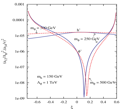
Figure 1: Comparison of radion (marked $\phi^{\prime}$) and higgs (marked $h^{\prime}$) couplings to the fermions or gauge bosons as defined in eq. (6). The used mass parameters are $m_{h}=150$ GeV and $m_{\phi}=250,500$ GeV.

The effects of mixing on the higgs and radion couplings to fermions and gauge bosons are presented in fig. 1, see eq. (6) for the definitions of $(a_{34}/v)$ and $(a_{12}/\Lambda_{\phi})$. From the figure it is evident that apart from the region around the special value of $\xi=\frac{1}{6}$, radion couplings to gauge bosons or fermions are bigger than the respective higgs couplings. Far enough from $|\xi|=\frac{1}{6}$, $\phi^{\prime}$ couplings are enhanced over the $h^{\prime}$ couplings. This phenomenon is purely due to the nature of the higgs-radion mixing. While calculating the radion (higgs) couplings, we have fixed $m_{h}=150$ GeV and $m_{\phi}=250$ or 500 GeV.

The couplings to gluons can be written as follows [13]:

$${\cal L}_{gg}=\left[\frac{1}{\Lambda_{\phi}}\left(\frac{{\cal M}_{11}}{Z_{R}}b_{3}-\frac{1}{2}a_{12}F_{1/2}(\tau_{t})\right)\phi^{{}^{\prime}}+\frac{1}{v}\left(\gamma\frac{{\cal M}_{12}}{Z_{R}}b_{3}-\frac{1}{2}a_{34}F_{1/2}(\tau_{t})\right)h^{{}^{\prime}}\right]\frac{\alpha_{s}}{8\pi}G_{\mu\nu}^{a}G^{\mu\nu a}$$ (7)

where $b_{3}$ is the QCD $\beta$-function coefficient. $F_{1/2}$ is the form factor from (heavy quark) loop effects. In each of these couplings the first term proportional to $b_{3}$ is coming from the trace anomaly. We can see from eq. (7) that the vertices higgs/radion -gluon-gluon have new contributions, which change the production and decay of the higgs boson. Couplings of radion/higgs to a pair of photons can also have anomalous contributions which we do not write here explicitly and which can be found elsewhere [13]. We do not write either the trilinear couplings involving radion and a pair of higgs or vice-versa, as we are not interested in these couplings in this work.

Without going into further details of the gluon couplings, we choose to plot in fig. 2 the radion branching ratio to gluons for both vanishing and non-zero values of $\xi$. For purpose of comparison we also present the same branching ratios for the higgs boson. For $\xi=0$, $\phi\rightarrow gg$ branching ratio is almost two orders of magnitude higher than the same for $h$. The sharp fall of the branching ratio around 160 GeV can be accounted for by the opening up of $WW$ decay modes. The radion branching ratio to a pair of gluons remains almost unchanged with mass, once the $WW$ threshold is crossed. For non-zero value of the mixing parameter the branching ratio rises with the radion mass. This is in sharp contrast with the higgs case. Higgs branching ratio to gluons in presence of mixing tends to decrease from its SM value for heavy $h^{{}^{\prime}}$.

Figure 2: Radion and higgs branching ratios for $\xi=1/6$ and $\xi=0$ for $\Lambda_{\phi}=1$  TeV. Whenever required we fix the radion and higgs mass parameters at 150 GeV.

What should we look for at a linear collider? The lesson we have learnt from previous discussion is that the radion coupling to a pair of gluons is enhanced due to the trace anomaly. This has been exploited in previous studies on radion production at hadronic colliders. The aim of the present work is to see the feasibility of next generation high energy $e^{+}e^{-}$ collider to differentiate between the Randall-Sundrum type models with radions and SM. As radion to photon photon coupling is also enhanced slightly (due to the modest running of QED $\beta$-function), possibilities of producing radions in photon photon collision (with back-scattered photons, using laser and high-energy electron or positron beams) have been considered [13]. This cross-section is not very impressive. Moreover, SM higgs has same kind of production and decay channel with almost competing strength. Thus, this production mode may not be suitable to differentiate between higgs and radion. This is why we turn to the process $e^{+}e^{-}\rightarrow\nu\bar{\nu}\phi(\rightarrow gg)$. We consider both the $WW$ fusion, which is the dominant production mechanism for the linear collider c.m. energies, and radion strahlung, $e^{+}e^{-}\rightarrow Z^{*}\rightarrow Z\phi$. Two jets in the final state are easier to deal with at an $e^{+}e^{-}$ machine than in a hadron collider. At the same time, radion branching ratio to gluons does not fall steadily with its mass apart from a sudden decrease around $2W/2Z$ threshold. This is related to the fact that radion gluon gluon coupling is independent of radion mass while for higgs the corresponding coupling decreases rather sharply with increased higgs mass. This is crucial in our analysis in the sense that unlike the higgs, gluon gluon branching ratio of radion can be substantial at high radion mass.

Moreover, for $\xi=0$, radion production via $WW$ fusion is suppressed due to the factor $(v/\Lambda_{\phi})$ in the coupling, with respect to higgs production in the same channel. Thus we have to be careful to choose such a decay channel for radion that this suppression factor can be overcome. This leads us to choose the radion decay to a pair of gluons. Even for $\xi\neq 0$, we can see from fig. 1 that for a wide (allowed) range of $\xi$ and radion mass, the radion coupling to a pair of $W$’s is larger than the same for higgs. This in turn implies the higher radion cross-section even at $\Lambda_{\phi}=1$  TeV. On the other hand, when $\phi^{\prime}-W-W$ coupling is small (around $\xi=1/6$), radion branching ratio to gluon gluon becomes big. This compensates the suppression in production. This already proves the efficacy of this particular channel.

We already mentioned that in the limit $\xi\rightarrow 0$, $\phi^{\prime}$ can be identified with the radion. In this work we will discuss the detection of $\phi^{\prime}$ through $gg$ decay. We will not present the other decay branching ratios of $\phi^{\prime}$ here. These can be obtained from our earlier works [7].

We have calculated the cross-section for $e^{+}e^{-}\rightarrow\nu\bar{\nu}\phi^{\prime}$ (all three $\nu$-flavours are added appropriately) and multiply by $\phi^{\prime}$ branching ratio to a pair of gluons. SM higgs boson has this decay mode as well and produce similar kind of a signal. On the other hand, higgs decay rate to gluons is suppressed w.r.t radions as discussed earlier. For the purpose of comparison we have also calculated the two-jet + missing energy yield in $e^{+}e^{-}$ collision via SM higgs production and decay. For low mass (around 100 GeV), the SM higgs decays dominantly to a pair of b-quarks, thus also producing two jets. If we assume a good b-jet identification/discrimination at a linear collider and veto any b-jet, this gives us a handle to discriminate the SM higgs from radion (around 100 GeV higgs/radion mass). We have also estimated the cross-section of two jets + missing momentum final state coming from $e^{+}e^{-}\rightarrow\nu\bar{\nu}\;(\gamma^{\ast},Z^{\ast},Z\rightarrow)\;q\bar{q}$. The strategy is to compare the invariant mass distribution of the jet pair. For radion one expects to have a peak around the radion mass we are interested in. On the other hand, the SM mass distribution of the jet pair has a continuum apart from a bump around $Z$-mass due to the on-shell $Z$-production. Two-jet mass distribution also peaks at low mass (of two jets), corresponding to the soft singularity associated with the $q\bar{q}$-pairs fragmented from a soft photon. We have used the following kinematic cuts on signal and SM background.

• for two jets $|p_{T}|>15$ GeV and $|\eta_{j}|\leq 3.0$.

• $\Delta r_{jj}\left(\equiv\sqrt{\Delta\eta_{jj}^{2}+\Delta\phi_{jj}^{2}}\right)>0.7$.

• ${p_{T}}\!\!\!\!\!\!/\;\;\;>15$ GeV.

There is one more contrasting feature of signal and background which helps us to reduce the background rate without affecting the signal too much. There is a dominant part of the background in which the neutrinos are coming from an on-shell $Z$. This can be easily seen from the missing mass distribution of signal and background as plotted in fig. 3. Around 90 GeV, the signal distribution also shows a bump, corresponding to the radion production in association with a real Z. We can eliminate a part of the background by imposing a further cut on the missing mass: $m_{mis}>120$ GeV. However, the dominant part of the background remains, and it has similar topology with the signal events.

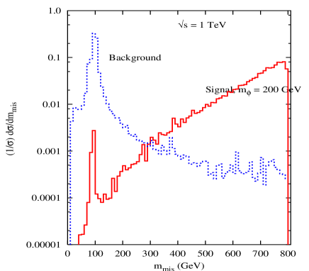
Figure 3: Missing mass distribution of signal and background.

In fig. 4 we have plotted the number of events against the two-jet invariant mass assuming an integrated luminosity of 500 fb^-1. For radion production the two jet invariant mass corresponds to the radion mass. When calculating the scatter plots, we have fixed the higgs mass parameter in the Lagrangian, $m_{h}=150$ GeV, and we have varied the radion mass parameter in the range 50 GeV$<m_{\phi}<$ 800 GeV, as well as the mixing parameter in the range $-0.75<\xi<0.59$. For the sake of comparison we have also plotted the corresponding numbers for the SM higgs boson (dotted lines), and for the radion in the nonmixed case, $\xi=0$ (dashed lines). The upper histogram line shows the background coming from the processes discussed above. For the detection the ratio of the signal $S$ to the background $B$ should be $S/\sqrt{B}>5$. The lower histogram line represents $5\sqrt{B}$. Thus a $5\sigma$ detection can be done if the parameter space point, marked by $+$ is above the lower histogram line. As expected, the cross-sections for both signal and background grow with the center-of mass energy. The sudden decrease of the radion cross-section around $m_{\phi^{\prime}}=$160 GeV is a reflection of decrement of $\phi^{\prime}\rightarrow gg$ branching ratio due to the opening up of $WW$ decay channel. A local peak in the SM higgs contribution (only seen in $\sqrt{s}=3$ TeV panel), around 350 GeV of mass of the jet pair (same as the higgs mass) is due to the opening up of the top-pair threshold to the $h-g-g$ coupling, via top loop.

We can estimate the detection possibilities with radion VEVs other than 1 TeV, by noticing that the cross-sections behave approximately as $1/\Lambda_{\phi}^{2}$. This is evident from eqn. 6. The $\phi^{\prime}gg$ coupling also depends on $\Lambda_{\phi}$, but the branching ratio of $\phi^{\prime}\rightarrow gg$ is almost insensitive to radion vev. Note that, apart from an overall $\frac{1}{\Lambda_{\phi}}$ in the couplings, quantities like $a_{12},\theta$ etc. also depends on this vev. Thus it is easy to conclude that for $\Lambda_{\phi}=3$ TeV, a very small region of the parameter space (mainly for $m_{\phi^{\prime}}<200$ GeV)would still be available with $\sqrt{s}=1$ TeV and a slightly larger region with $\sqrt{s}=3$ TeV. $\Lambda_{\phi}=5$ TeV or above cannot be detected by any of the studied center of mass energies.

We have not separately presented the numbers for $h^{\prime}$. However, one can see from the general arguments that $h^{\prime}$ production with a neutrino pair and the consequent decay to $gg$, is suppressed with respect to the $\phi^{\prime}$.

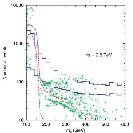
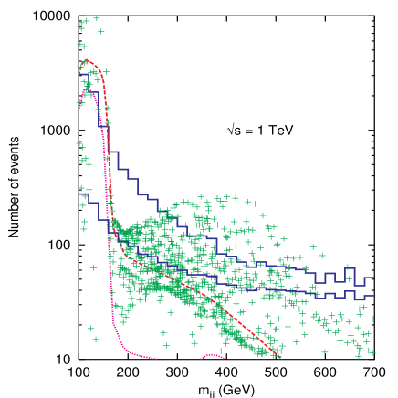
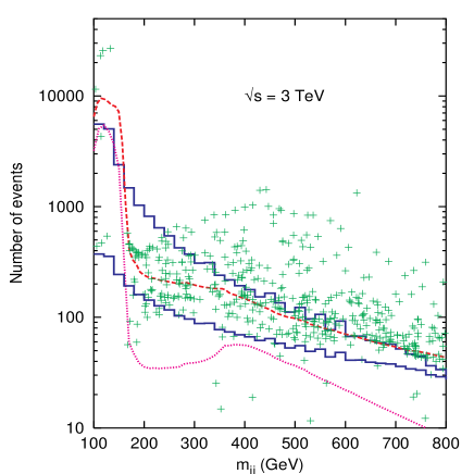
Figure 4: Number of signal ($+$ for $\xi\neq 0$ and dashed line is for $\xi=0$), SM higgs (dotted line) and background (solid histogram) events as a function of the invariant mass of the jets. The upper histogram hows the actual number of background events. The lower histogram shows the 5$\sigma$ fluctuation of background. Points (representing the signal from higgs and radion) above the lower histogram can be explored at 5$\sigma$. Whenever required we fix the higgs mass parameter at 150 GeV.

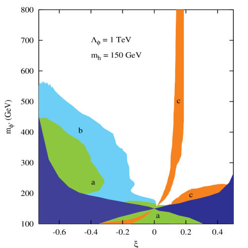
Figure 5: Radion mass reach as a function of the mixing parameter $\xi$. Radion masses, corresponding to the dark wedge-shaped regions on both sides of $\xi=0$, are not allowed. Regions (triangular area close to $\xi=0$ and in the left side) marked with $a$, can be probed at $5\sigma$ level with $e^{+}e^{-}$ center of mass energy 800 GeV. Region marked with $b$ along with $a$ can be probed at $5\sigma$ level with $e^{+}e^{-}$ center of mass energy 1 TeV. The white regions along with $a$ and $b$ can be probed with 3 TeV $e^{+}e^{-}$ center of mass energy. In the shaded regions marked with $c$ (note that there is a small region $c$ close to $\xi=0$ but for $\xi<0$) either the radion production is too small or the $gg$ decay branching ratio is too small. These regions cannot be probed.

It is evident from fig. 1 that $h^{\prime}$ production via $WW$ fusion is less sensitive to $\xi$, than $\phi^{\prime}$. The production rate is always suppressed w.r.t the $\phi^{\prime}$, except for $\xi$ values close to $\frac{1}{6}$. For $\xi$ values close to 1/6, $\phi^{\prime}$ branching ratio to gluons is orders of magnitude larger than the same for $h^{\prime}$. We have explicitly checked that number of 2 jet + missing energy events coming form $h^{\prime}$ production and decay can only be above the 5$\sigma$ fluctuation of the SM background when higgs mass is below the $WW$ threshold. Thus, in general one may see two resonances below the $WW$ threshold, but presence of a single resonance (in gluon gluon invariant mass distribution) with mass greater than 200 GeV, definitely points towards the presence of extra scalar like radion.

It is evident from the figures 4 that radion-higgs mixing has a very positive effect on the radion search. As for example, with 800 GeV and 1 TeV center-of-mass energy, our proposed signal can test radion mass up to say 200 GeV in the no-mixing case. When the mixing is put on, this mass reach is certainly improved for favorable cases. For all the examples in fig. 4, the radion cross-section is well above the higgs cross-section for $\xi=0$ case, while non-zero values of $\xi$ can push the cross-section in both ways with respect to the no-mixing case.

The above three figures can be nicely summarised in a single plot, depicting the regions (in $\xi-m_{\phi^{\prime}}$ plane) in which the proposed signal is significantly above the background. In fig. 5, we have identified the regions where the numbers of signal events are more than five times the square root of the background. The negative values of mixing seem to be favorable to probe heavier radions for lower center of mass energies. In the shaded regions marked with $a$ and $b$ along with white region, the signal strength is higher than the 5$\sigma$ fluctuation of the background. One can claim a discovery of radions in these regions of the parameter space. Regions marked with $a$ can be probed by a 800 GeV linear collider and regions marked with $b$ by a 1 TeV linear collider. To probe the white regions, a 3 TeV linear collider is required. In the shaded region marked with $c$, (due to conspiracy of either the radion coupling to $WW/ZZ$ or to $gg$) signal is too weak compared with the background even at an $e^{+}e^{-}$ center of mass energy of 3 TeV. In fact, in the shaded region (marked c) parallel to the $m_{\phi^{\prime}}$ axis, around $\xi=1/6$, the radion production is too small. This can be accounted for by the small coupling of the radion to $WW/ZZ$ as evident from fig. 1. A larger radion branching ratio to gluons in this region cannot compensate to yield a signal strength comparable with background. In the dark wedge shaped regions, no physical values for radion masses ($m_{\phi^{\prime}}$) are possible for any input parameters. This can be explained from the definition of mixing angle $\theta$ (see eqn.4) in terms of other input parameters.

To summarise, we have investigated the possible signature of radions in Randall-Sundrum scenario at future $e^{+}e^{-}$ colliders. If nature chooses the Randall-Sundrum type of geometry of space and time, then radion, the lowest lying gravitational excitation in this scenario, can be explored at the hadronic collider like LHC. Being a graviscalar, it couples to the SM particles via the trace of the energy-momentum tensor. This implies that the couplings are very similar to that of the SM higgs boson. One important difference from higgs is the gluon gluon coupling, which is enhanced for radions due to conformal anomaly. It is important to look not only for the possible signatures for this scalar particle at future $e^{+}e^{-}$ machines, but also to differentiate this from the SM higgs boson. We propose to look for the process in which radion is dominantly produced via $WW$ fusion in $e^{+}e^{-}$ collision along with neutrinos and subsequently decays to a pair of gluons. This in the final state produces 2 jet + missing momentum signature, with a peak in two jet mass distribution. We have also estimated the contribution to this final state from SM higgs boson and also from other SM backgrounds. Though at an $e^{+}e^{-}$ collider with $\sqrt{s}=500$ GeV the detection is not obvious, at $\sqrt{s}=800$ GeV and above one can expect $5\sigma$ effect in exploring the radion and differentiating it from the SM higgs boson.

Acknowledgments: Authors thank the Academy of Finland (project number 48787) for financial support.

References

- [1] N. Arkani-Hamed, S. Dimopoulos and G. Dvali, Phys. Lett. B429 (1998) 263; N. Arkani-Hamed, S. Dimopoulos and G. Dvali, Phys. Lett. B436 (1998) 257.
- [2] L. Randall and R. Sundrum, Phys. Rev. Lett. 83 (1999) 3370; L. Randall and R. Sundrum, Phys. Rev. Lett. 83 (1999) 4690.
- [3] W.D. Goldberger and M.B. Wise, Phys. Rev. Lett. 83 (1999) 4922; W.D. Goldberger and M.B. Wise, Phys. Rev. D60 (1999) 107505.
- [4] M. Luty and R. Sundrum, Phys. Rev. D62 (2000) 035008.
- [5] C. Csaki, M. Graesser, L. Randall and J. Terning, Phys. Rev. D62 (2000) 045015.
- [6] W.D. Goldberger and M.B. Wise, Phys. Lett. B475 (2000) 275.
- [7] U. Mahanta and S. Rakshit, Phys. Lett. B480 (2000) 176; U. Mahanta and A. Datta, Phys. Lett. B483 (2000) 196; K. Cheung, Phys.Rev.D 63 (2001) 056007; S. Bae, P. Ko, H.S. Lee and J. Lee, Phys. Lett. B487 (2000) 299; S. Bae, and H.S. Lee, hep-ph/0011275; M. Chaichian, A. Datta, K. Huitu, Z.H. Yu, Phys. Lett. B524 (2002) 161; P. Das, U. Mahanta, Nucl. Phys. B644 (2002) 395; Phys.Lett. B528 (2002) 253, A. Gupta, N. Mahajan, Phys.Rev. D65 (2002) 056003; P. Das, B. Mukhopadhyaya, hep–ph/0303135.
- [8] T. Han, G. D. Kribs, and B. McElrath, Phys. Rev. D64 (2001) 076003; D. Choudhury, S.R. Choudhury, A. Gupta and N. Mahajan Jour. Phys. G28, 1191 (2002).
- [9] K. Cheung, C. S. Kim, J-H. Song, hep–ph/0301002.
- [10] D. Dominici, B. Grzadkowski, J. Gunion and M. Toharia, hep–ph//0206192; Acta. Phys. Polon. B33 (2002) 2507; M. Battaglia et al., hep–ph//0304245.
- [11] G.F. Giudice, R. Rattazzi and J.D. Wells, Nucl. Phys. B 595 (2001) 250.
- [12] C. Csaki, M. Graesser and G. Kribs, Phys. Rev. D63 (2001) 065002.
- [13] M. Chaichian, K. Huitu, A. Kobakhidze and Z.-H. Yu, Phys. Lett.B 515 (2001) 65; S.R. Choudhury, A.S. Cornell and G.C. Joshi, hep-ph/0012043.