Abstract

The original B. Pontecorvo idea of neutrino oscillations is discussed. Neutrino mixing and basics of neutrino oscillations in vacuum and in matter are considered. Recent evidences in favour of neutrino oscillations, obtained in the Super-Kamiokande, SNO, KamLAND and other neutrino experiments are discussed. Neutrino oscillations in the solar and atmospheric ranges of the neutrino mass-squared differences are considered in the framework of the minimal scheme with the mixing of three massive neutrinos. Results of the tritium $\beta$-decay experiments and experiments on the search for neutrinoless double $\beta$-decay are briefly discussed.

1 Pontecorvo idea of neutrino oscillations

B. Pontecorvo came to the idea of neutrino oscillations in 1957, soon after parity violation in $\beta$-decay was discovered by Wu et. al. [1] and the two-component theory of massless neutrino was proposed by Landau [2], Lee and Yang [3] and Salam [4].

For the first time B.Pontecorvo mentioned the possibility of neutrino $\rightleftarrows$ antineutrino transitions in vacuum in his paper [5] on muonium $\rightleftarrows$ antimuonium transition ($\mu^{-}e^{+}\rightleftarrows\mu^{+}e^{-}$). He believed in the analogy between the weak interaction of leptons and hadrons and looked in the lepton world for a phenomenon that would be analogous to $K^{0}\rightleftarrows\overline{K}{{}^{0}}$ oscillations. In his work of 1957 [5] B. Pontecorvo wrote:

“If the two-component neutrino theory should turn out to be incorrect (which at present seems to be rather improbable) and if the conservation law of neutrino charge would not apply, then in principle neutrino $\leftrightarrow$ antineutrino transitions could take place in vacuum.”

B. Pontecorvo wrote his first paper on neutrino oscillations later in 1958 [6] at the time when F. Reines and C. Cowan [7] had just finished the famous reactor experiment, which led them to discover the electron antineutrino through the observation of the inverse $\beta$-process

$$\overline{\nu}_{e}+p\rightarrow e^{+}+n\,.$$ (1)

At that time R. Davis was doing an experiment with reactor antineutrinos [8]. R.Davis searched for production of  ${}^{37}\rm{Ar}$ in the process

$$\overline{\nu}_{e}+\,^{37}\rm{Cl}\rightarrow e^{-}+\,^{37}\rm{Ar}\,,$$ (2)

which is allowed only if the lepton number is not conserved. A rumor reached B. Pontecorvo that R. Davis had seen some events (2). B.Pontecorvo, who had earlier been thinking about possible antineutrino $\rightleftarrows$ neutrino transitions, decided to study this possibility in details.

“Recently the question was discussed [5] whether there exist other mixed neutral particles beside the $K^{0}$ mesons, i.e., particles that differ from the corresponding antiparticles, with the transitions between particle and antiparticle states not being strictly forbidden. It was noted that the neutrino might be such a mixed particle, and consequently there exists the possibility of real neutrino $\leftrightarrow$ antineutrino transitions in vacuum, provided that lepton (neutrino) charge is not conserved. This means that the neutrino and antineutrino are mixed particles, i.e., a symmetric and antisymmetric combination of two truly neutral Majorana particles $\nu_{1}$ and $\nu_{2}$ of different combined parity”

In Ref. [6] B. Pontecorvo wrote that he has considered this possibility

“… since it leads to consequences which, in principle, can be tested experimentally. Thus, for example, a beam of neutral leptons consisting mainly of antineutrinos when emitted from a nuclear reactor, will consist at some distance $R$ from the reactor of half neutrinos and half antineutrinos.”

In 1958 only the electron neutrino was known. In Ref. [6] B. Pontecorvo considered oscillations of the active right-handed antineutrino to a right-handed neutrino, the only possible oscillations in the case of one type of neutrino. In this paper, that was written at a time when the two-component neutrino theory had just appeared and the Davis reactor experiment was not yet finished, B. Pontecorvo discussed a possible explanation of the Davis “events”. Later B. Pontecorvo understood that in the framework of the two-component neutrino theory, established after M. Goldhaber et al. experiment [9], right-handed neutrinos are practically sterile particles. B. Pontecorvo was in fact the first, who introduced the notion of sterile neutrinos in Ref. [10].

B.Pontecorvo stressed [6] that if the oscillation length $R$ is large, it will be difficult to observe the effect of the neutrino oscillations in reactor experiments. He wrote:

“Effects of transformation of neutrino into antineutrino and vice versa may be unobservable in the laboratory because of the large values of R, but will certainly occur, at least, on an astronomical scale.”

B. Pontecorvo came back to the consideration of neutrino oscillations in 1967 [10]. At that time the phenomenological V-A theory of Feynman and Gell-Mann [12], Marshak and Sudarshan [13] was established and in the Brookhaven experiment [14], which was proposed by B.Pontecorvo in 1959 [15], it was proved that (at least) two types on neutrinos $\nu_{e}$ and $\nu_{\mu}$ exist in nature. B.Pontecorvo confidence in nonzero neutrino masses and neutrino oscillations became stronger after these findings.

In Ref. [10] B.Pontecorvo discussed experiments in which conservation of lepton numbers were tested and came to the conclusion that there is “plenty of room for violation of lepton numbers, especially in pure leptonic interactions”. He formulated [6, 10] the conditions at which neutrino oscillations are possible:

1. Lepton numbers, conserved by the usual weak interaction, are violated by an additional interaction between neutrinos.

2. Neutrino masses are different from zero.

In modern terminology these conditions are equivalent to the assumption that in the total Lagrangian there is a neutrino mass term, non-diagonal in flavour neutrino fields.

In Ref. [10] B. Pontecorvo considered different lepton numbers in the case of two types of neutrinos: additive electron and muon lepton numbers $L_{e}$ and $L_{\mu}$, ZKM lepton number [16] equal to 1 for $e^{-}$ and $\mu^{+}$ and -1 for $e^{+}$ and $\mu^{-}$ etc. He stressed that if violation of $L_{e}$ and $L_{\mu}$ occurs, in addition to the oscillations between active flavour neutrinos $\nu_{\mu}\rightleftarrows\nu_{e}$ oscillations between active and sterile neutrinos ( $\nu_{\mu}\leftrightarrow\bar{\nu}_{\mu L}$, $\nu_{e}\rightleftarrows\bar{\nu}_{\mu L}$ etc) become possible.

In the case of ZKM lepton number $L$ for one four-component neutrino $\nu$ we have the following correspondence: $\nu_{L}\equiv\nu_{e}$, $\nu_{R}\equiv\bar{\nu}_{\mu}$, $\bar{\nu}_{L}\equiv\nu_{\mu}$, $\bar{\nu}_{R}\equiv\bar{\nu}_{e}$. If the interaction between neutrinos does not conserve $L$, only transitions between active neutrinos ($\nu_{L}\rightleftarrows\bar{\nu}_{L}$ and $\nu_{R}\rightleftarrows\bar{\nu}_{R}$) are then possible.

In his work of 1967 [10] B. Pontecorvo discussed the oscillations of solar neutrinos. At that time R. Davis started his famous experiment on the detection of the solar neutrinos. The experiment was based on the radiochemical method, proposed by B. Pontecorvo in 1946 [11]. Solar neutrinos were detected via the observation of the Pontecorvo-Davis reaction

$$\nu_{e}+\,^{37}\rm{Cl}\rightarrow e^{-}+\,^{37}\rm{Ar}.$$ (3)

Quite remarkably, in [10] B. Pontecorvo envisaged the solar neutrino problem. Indeed, before the first results of Davis experiment were obtained, he wrote:

“From an observational point of view the ideal object is the sun. If the oscillation length is smaller than the radius of the sun region effectively producing neutrinos, (let us say one tenth of the sun radius $R_{\odot}$ or 0.1 million km for ${}^{8}B$ neutrinos, which will give the main contribution in the experiments being planned now), direct oscillations will be smeared out and unobservable. The only effect on the earth’s surface would be that the flux of observable sun neutrinos must be two times smaller than the total (active and sterile) neutrino flux.”

It was shown by Gribov and Pontecorvo in 1969 [17] that in the neutrino mass term only active left-handed fields $\nu_{eL}$ and $\nu_{\mu L}$ can enter. The corresponding mass term is called Majorana mass term. Particles with definite masses are in this case Majorana neutrinos and flavour fields $\nu_{eL}$ and $\nu_{\mu L}$ are connected with the Majorana fields $\nu_{1L}$ and $\nu_{2L}$ by the mixing relation

$$\begin{array}[]{lll}\nu_{e}=\cos\theta\,~{}\nu_{1L}+\sin\theta\,~{}\nu_{2L};\\ &&\\ \nu_{\mu}=-\sin\theta\,~{}\nu_{1L}+\cos\theta\,~{}\nu_{2L},\end{array}$$ (4)

where $\theta$ is the mixing angle.

In Ref. [17] the expression for the survival probability of $\nu_{e}$ was obtained and oscillations of solar neutrinos in vacuum were considered.

In the seventies the Cabibbo-GIM mixing of $d$ and $s$ quarks was established. In Ref. [18] neutrino oscillations in the scheme of the mixing of two Dirac neutrinos $\nu_{1}$ and $\nu_{2}$ were considered. This scheme was based on the analogy between quarks and leptons. In the same work possible values of the mixing angle $\theta$ were discussed:

“…it seems to us that the special values of mixing angle $\theta=0$ (the usual scheme in which muonic charge is strictly conserved) and $\theta=\pi/4$ are of the greatest interest. ”

Neutrino oscillations and in particular solar neutrino oscillations were considered in Ref. [19] in the general case of the Dirac and Majorana mass term: the latter does not conserve any lepton numbers. It is built from active left-handed fields $\nu_{lL}$ and sterile right-handed fields $\nu_{lR}$.

In 1978 the first review on neutrino oscillations was published [20]. At that time the list of papers on neutrino oscillations was very short: except for the cited papers of B. Pontecorvo and his collaborators, it included only references [21, 22, 23, 24, 25] and [26, 27]. The review attracted the attention of many physicists to the problem of neutrino mass and neutrino oscillations. In particular, it was stressed in this review that due to the interference character of neutrino oscillations the investigation of this phenomenon is the most sensitive method to search for small neutrino mass-squared differences.

During the preparation of the review [20] the authors became familiar with the work of Maki et al. [21], which was unknown to many physicists for many years. In this paper, in the framework of the Nagoya model, in which $p$, $n$ and $\Lambda$ were considered as bound states of some vector particle $B^{+}$ and leptons, the mixing of two neutrinos was introduced. In addition to the usual neutrinos $\nu_{e}$ and $\nu_{\mu}$, which they called weak neutrinos, the authors introduced massive neutrinos $\nu_{1}$ and $\nu_{2}$, which they called true neutrinos. In the Nagoya model the proton was considered as a bound state of the $B^{+}$ and the neutrino $\nu_{1}$.

Maki, Nakagawa and Sakata assumed that the fields of weak neutrinos and of true neutrinos are connected by an orthogonal transformation:

“It should be stressed at this stage that the definition of the particle state of the neutrino is quite arbitrary; we can speak of neutrinos which are different from weak neutrinos but are expressed by a linear combination of the latter. We assume that there exists a representation which defines the true neutrinos through some orthogonal transformation applied to the representation of weak neutrinos:

$$\begin{array}[]{lll}\nu_{1}&=&+\nu_{e}\cos\delta+\nu_{\mu}\sin\delta\\ &&\\ \nu_{2}&=&-\nu_{e}\sin\delta+\nu_{\mu}\cos\delta\;^{\prime\prime}\end{array}$$ (5)

In Ref. [21] neutrino oscillations, as a phenomenon based on the quantum mechanics of a mixed system, were not considered. In connection with the Brookhaven experiment [14], which was going on at that time, the authors wrote

“In the present case, however, weak neutrinos are not stable due to occurrence of virtual transmutation $\nu_{\mu}\rightarrow\nu_{e}$ induced by the interaction ${\cal L}=g\overline{\nu}_{2}\nu_{2}X^{+}X$ ($X$ is a field of heavy particles). If the mass difference between $\nu_{1}$ and $\nu_{2}$, i.e. $|m_{\nu_{2}}-m_{\nu_{1}}|=m_{\nu_{2}}$, is assumed to be a few MeV the transmutation time $T\left(\nu_{e}\leftrightarrow\nu_{\mu}\right)$ becomes $\sim$ $10^{-18}$ sec for fast neutrinos with momentum $\sim$ BeV$/c$.

Therefore a chain of reactions such as

$$\pi^{+} \rightarrow \mu^{+}\nu_{\mu}$$

$$\nu_{\mu}+Z\left(nucleus\right) \rightarrow Z^{\prime}+\left(\mu^{-}\;/\;e^{-}\right)$$ (6)

is useful to check the two-neutrino hypothesis only when $|m_{\nu_{2}}-m_{\nu_{1}}|\leq 10^{-6}$ MeV under the conventional geometry of the experiments. Conversely, the absence of $e^{-}$ in the reaction (6) will be able not only to verify two-neutrino hypothesis but also to provide an upper limit of the mass of the second neutrino $\nu_{2}$ if the present scheme should be accepted.”

Recently very strong, convincing evidence in favour of neutrino oscillations, which we will discuss later, were obtained. It required many years of work and heroic efforts of many experimental groups to reveal the effects of tiny neutrino masses and neutrino mixing. From our point of view it is a proper time to give a tribute to the great intuition of B. Pontecorvo, who pursued the idea of neutrino oscillations for many years at a time when the general opinion, mainly based on the success of the two-component neutrino theory, favoured massless neutrinos . The history of neutrino oscillations is an illustration of the importance of analogy in physics. It is also an illustration of the importance of new courageous ideas, not always in agreement with the general opinion.

2 Introduction

Convincing evidence of neutrino oscillations was obtained in the last 4-5 years in experiments with neutrinos from natural sources: in the atmospheric [29, 30, 31] and solar neutrino experiments [32, 33, 34, 35, 36, 37, 38]. Recently strong evidence in favour of neutrino oscillations was obtained in the reactor KamLAND experiment [39].

The observation of neutrino oscillations implies that neutrino masses are different from zero and that the states of flavour neutrinos $\nu_{e},\nu_{\mu},\nu_{\tau}$ are coherent superpositions (mixtures) of the states of neutrinos with definite masses. All existing data, including astrophysical ones, suggest that neutrino masses are much smaller than the masses of leptons and quarks. The smallness of neutrino masses is a signature of a new, beyond the Standard Model, physics.

In this review we present the phenomenological theory of neutrino masses and mixing and the see-saw mechanism of neutrino mass generation [40]. We consider neutrino oscillations in vacuum and transitions between different flavour neutrinos in matter. Then we will discuss the recent experimental evidence in favour of neutrino oscillations: the results of the Super-Kamiokande atmospheric neutrino experiment [29], in which a significant up-down asymmetry of the high-energy muon events was observed, the results of the SNO solar neutrino experiment [36, 37, 38], in which a direct evidence for the transition of the solar $\nu_{e}$ into $\nu_{\mu}$ and $\nu_{\tau}$ was obtained and the results of the KamLAND experiment [39] in which the disappearance of the reactor $\bar{\nu}_{e}$ was observed. We will also discuss the long baseline CHOOZ  [41] and Palo Verde [42] reactor experiments in which no indications in favour of neutrino oscillations were obtained. Yet the results of these experiments are very important for neutrino mixing.

Neutrino oscillations in the atmospheric and solar ranges of neutrino mass-squared differences will be considered in the framework of three-neutrino mixing. We will show that neutrino oscillations in these two regions are practically decoupled and are described in the leading approximation by the two-neutrino formulas.

The investigation of neutrino oscillations is based on the following assumptions, which are supported by all existing experimental data.

1. The interaction of neutrinos with other particles is described by the Standard Model of the electroweak interaction.

   The Standard Charged Current (CC) and Neutral Current (NC) Lagrangians are given by

   $$\mathcal{L}_{I}^{\mathrm{CC}}=-\frac{g}{2\sqrt{2}}\,j^{\mathrm{CC}}_{\alpha}\,W^{\alpha}+\mathrm{h.c.};\,~{}~{}\mathcal{L}_{I}^{\mathrm{NC}}=-\frac{g}{2\cos\theta_{W}}\,j^{\mathrm{NC}}_{\alpha}\,Z^{\alpha}\,.$$ (7)

   Here $g$ is the SU(2) gauge coupling constant, $\theta_{W}$ is the weak angle, $W^{\alpha}$ and $Z^{\alpha}$ are the fields of the charged ($W^{\pm}$) and neutral ($Z^{0}$) vector bosons and the leptonic charged current $j^{\mathrm{CC}}_{\alpha}$ and neutrino neutral current $j^{\mathrm{NC}}_{\alpha}$ are given by the expressions:

   $$j^{\mathrm{CC}}_{\alpha}=2\,\sum_{l}\bar{\nu}_{lL}\gamma_{\alpha}l_{L};\,~{}~{}j^{\mathrm{NC}}_{\alpha}=\sum_{l}\bar{\nu}_{lL}\gamma_{\alpha}\nu_{lL}\,.$$ (8)

2. Three flavour neutrinos $\nu_{e}$, $\nu_{\mu}$ and $\nu_{\tau}$ exist in nature.

   From the LEP experiments on the measurement of the width of the decay $Z\to\nu+\bar{\nu}$ the following value was obtained [43] for the number of flavour neutrinos $n_{\nu_{f}}$:

   $$n_{\nu_{f}}=3.00\pm 0.06$$ (9)

   and from the global fit of the LEP data the value

   $$n_{\nu_{f}}=2.984\pm 0.008.$$ (10)

   was found.

3 Neutrino masses and mixing

If neutrino fields enter only in the Standard Model (SM) Lagrangians (7), neutrinos are massless particles and the three flavour lepton numbers, electron ($L_{e}$), muon ($L_{\mu}$) and tau ($L_{\tau}$), are separately conserved. The hypothesis of neutrino mixing is based on the assumption that in the total Lagrangian there is a neutrino mass term, which does not conserve flavour lepton numbers. Several mechanisms of the generation of the neutrino mass term were proposed. In this section we will discuss the most plausible see-saw mechanism [40].

Let us start with the phenomenological theory of the neutrino masses and mixing. There are two types of possible neutrino mass terms (see [44, 45]).

1. Dirac mass term

   $$\mathcal{L}^{\mathrm{D}}=-\bar{\nu}^{\prime}_{R}\,M^{\mathrm{D}}\nu^{\prime}_{L}+\mathrm{h.c.}$$ (11)

   Here

   $$\nu^{\prime}_{L}=\left(\begin{array}[]{c}\nu_{eL}\\ \nu_{\mu L}\\ \nu_{\tau L}\\ \vdots\end{array}\right);\,~{}\nu^{\prime}_{R}=\left(\begin{array}[]{c}\nu_{eR}\\ \nu_{\mu R}\\ \nu_{\tau R}\\ \vdots\end{array}\right)$$ (20)

   and $M^{\mathrm{D}}$ is a complex non-diagonal matrix. We assume that in the column $\nu^{\prime}_{L}$ not only left-handed flavour neutrino fields $\nu_{eL},\nu_{\mu L},\nu_{\tau L}$ but also sterile fields could enter. Sterile fields do not enter into the standard charged and neutral currents (see discussion later).

   The matrix $M^{\mathrm{D}}$ can be diagonalized by a bi-unitary transformation. We have (see [44, 45]):

   $$M^{\mathrm{D}}=V\,m\,U^{+},$$ (21)

   where $V$ and $U$ are unitary matrices and $m_{ik}=m_{i}\,\delta_{ik};\,m_{i}>0$. From Eq. (11) and Eq. (21) for the neutrino mass term we obtain the standard expression

   $$\mathcal{L}^{D}=-\sum_{i}m_{i}\,\bar{\nu}_{i}\nu_{i},$$ (22)

   where $\nu_{i}$ is the field of neutrino with mass $m_{i}$.

   The flavour field $\nu_{lL}$ is connected with left-handed field $\nu_{iL}$ by the mixing relation

   $$\nu_{lL}=\sum_{i}U_{li}\nu_{iL}\,.$$ (23)

   It is obvious that the total Lagrangian is invariant under the global gauge transformation

   $$\nu^{\prime}_{L}\to e^{i\,\alpha}\,\nu^{\prime}_{L};\,\nu^{\prime}_{R}\to e^{i\,\alpha}\,\nu^{\prime}_{R};\,l\to e^{i\,\alpha}\,l\,$$

   where $\alpha$ is an arbitrary constant phase. From this invariance it follows that the total lepton number $L=\sum_{l}\,L_{l}$ is conserved and $\nu_{i}$ is the field of the Dirac neutrinos and antineutrinos with $L=1$ for neutrinos and $L=-1$ for antineutrinos.

2. Majorana mass term

   $$\mathcal{L}^{\mathrm{M}}=-\frac{1}{2}\,(\overline{\nu^{\prime}_{L}})^{c}\,M^{\mathrm{M}}\nu^{\prime}_{L}+\mathrm{h.c.}$$ (24)

   Here

   $$(\nu^{\prime}_{L})^{c}=C(\bar{\nu}^{\prime})^{T}_{L};\,~{}~{}(\overline{\nu^{\prime}_{L}})^{c}=-(\nu^{\prime})^{T}_{L}\,C^{-1},$$

   where $C$ is the charge conjugation matrix, which satisfies the conditions

   $$C\,\gamma^{T}_{\alpha}\,~{}~{}C^{-1}=-\gamma_{\alpha};\,~{}C^{T}=-C.$$

   The matrix $M^{\mathrm{M}}$ is a symmetrical matrix. In fact, taking into account the Fermi-Dirac statistics of the field $\nu^{\prime}_{L}$, we have

   $$(\overline{\nu^{\prime}_{L}})^{c}\,M^{\mathrm{M}}\nu^{\prime}_{L}=(\nu^{\prime}_{L})^{T}\,(C^{-1})^{T}(M^{\mathrm{M}})^{T}\nu^{\prime}_{L}=(\overline{\nu^{\prime}_{L}})^{c}\,(M^{\mathrm{M}})^{T}\nu^{\prime}_{L}\,.$$

   From this relation we obtain

   $$M^{\mathrm{M}}=(M^{\mathrm{M}})^{T}\,.$$

   For a symmetrical matrix we have (see [44, 45])

   $$M^{\mathrm{M}}=(U^{+})^{T}\,m\,U^{+},$$ (25)

   where $U$ is a unitary matrix and $m_{ik}=m_{i}\,\delta_{ik};\,~{}~{}m_{i}>0$.

   From Eqs.(24) and (25) it follows that the Majorana mass term takes the form

   $$\mathcal{L}^{M}=-\frac{1}{2}\,\sum_{i}m_{i}\,\bar{\nu}_{i}\nu_{i},$$ (26)

   where $\nu_{i}$ is the field of neutrino with mass $m_{i}$, which satisfies the Majorana condition

   $$\nu_{i}=\nu^{c}_{i}=C(\bar{\nu})^{T}_{i}.$$ (27)

   The flavour field $\nu_{lL}$ is connected with the Majorana fields $\nu_{iL}$ by the mixing relation

   $$\nu_{lL}=\sum_{i}U_{li}\nu_{iL}.$$ (28)

   In the case of the Majorana mass term there is no global gauge invariance of the total Lagrangian. Hence, Majorana neutrinos are truly neutral particles: they do not carry neither electric charge nor lepton numbers. In other words Majorana neutrinos and antineutrinos are identical particles.

If there are only flavour fields $\nu_{lL}$ in the column $\nu^{\prime}_{L}$, the number of the massive neutrinos $\nu_{i}$ is equal to the number of flavour neutrinos (three) and $U$ is a 3$\times$3 Pontecorvo-Maki-Nakagawa-Sakata (PMNS) [6, 10, 21] unitary mixing matrix.

If, in the column $\nu^{\prime}_{L}$, there are also sterile fields $\nu_{sL}$, the number of massive neutrinos $\nu_{i}$ will be larger than three. In this case the mixing relation takes the form

$$\nu_{lL}=\sum_{i=1}^{3+n_{s}}U_{li}\nu_{iL};\,~{}\nu_{sL}=\sum_{i=1}^{3+n_{s}}U_{si}\nu_{iL}\,,$$ (29)

where $n_{s}$ is the number of the sterile fields, $U$ is a unitary $(3+n_{s})\times(3+n_{s})$ matrix, $\nu_{i}$ is the field of neutrino with mass $m_{i}$ ($i=1,2,..,3+n_{s}$).

Sterile fields can be right-handed neutrino fields, SUSY fields etc. If more than three neutrino masses are small, the transition of the flavour neutrinos $\nu_{e}$, $\nu_{\mu}$, $\nu_{\tau}$ into sterile states becomes possible.

A special interest has the so-called Dirac and Majorana mass term. Let us assume that, in addition to the flavour fields $\nu_{lL}$, in the column $\nu^{\prime}_{L}$ also the fields $(\nu_{lR})^{c}$ ($l=e,\mu,\tau$) enter. The Majorana mass term (24) can then be presented in the form of the sum of the left-handed Majorana, Dirac and right-handed Majorana mass terms:

$$\mathcal{L}^{\mathrm{D+M}} = -\frac{1}{2}\,(\overline{\nu_{L}})^{c}\,M^{\mathrm{M}}_{L}\nu_{L}-\bar{\nu}_{R}\,M^{\mathrm{D}}\,\nu_{L}-\frac{1}{2}\,\bar{\nu}_{R}\,M^{\mathrm{M}}_{R}(\nu_{R})^{c}+\mathrm{h.c.}$$ (30)

$$= -\frac{1}{2}\,(\overline{\nu^{\prime}_{L}})^{c}\,M^{\mathrm{D+M}}\nu^{\prime}_{L}+\mathrm{h.c.}$$

Here

$$\nu_{L}=\left(\begin{array}[]{c}\nu_{eL}\\ \nu_{\mu L}\\ \nu_{\tau L}\end{array}\right),\,~{}\nu_{R}=\left(\begin{array}[]{c}\nu_{eR}\\ \nu_{\mu R}\\ \nu_{\tau R}\end{array}\right)\,,$$ (37)

$M^{\mathrm{M}}_{L}$ and $M^{\mathrm{M}}_{R}$ are complex non-diagonal symmetrical 3$\times$3 Majorana matrices and $M^{\mathrm{D}}$ is a complex non-diagonal 3$\times$3 Dirac matrix. After the diagonalization of the mass term (30) one gets

$$\nu_{lL}=\sum_{i=1}^{6}U_{li}\nu_{iL};\,~{}(\nu_{lR})^{c}=\sum_{i=1}^{6}U_{\bar{l}i}\nu_{iL},$$ (38)

where $U$ is the unitary 6$\times$6 mixing matrix and $\nu_{i}$ is the field of the Majorana neutrino with mass $m_{i}$.

The standard see-saw mechanism of the neutrino mass generation [40] is based on the assumption that the neutrino mass term is the Dirac and Majorana one, with $M_{L}^{\rm{M}}=0$. To illustrate this mechanism we will consider the simplest case of one type of neutrino. Let us assume that the standard Higgs mechanism with one Higgs doublet, which is the mechanism of generation of the masses of quarks and leptons, also generates the Dirac neutrino mass term

$$\mathcal{L}^{\mathrm{D}}=-m\,\bar{\nu}_{R}\nu_{L}+\mathrm{h.c.}$$ (39)

It is natural to expect that the mass $m$ is of the same order of magnitude of the lepton or quark masses in the same family. However, we know from experimental data that neutrino masses are much smaller than the masses of leptons and quarks. In order to “suppress” the neutrino mass we will assume that there is a beyond the SM, lepton number violating mechanism of generation of the right-handed Majorana mass term

$$\mathcal{L}^{\mathrm{M}}_{R}=-\frac{1}{2}\,M\,\bar{\nu}_{R}(\nu_{R})^{c}+\mathrm{h.c.},$$ (40)

with $M\gg m$ (usually it is assumed that $M\simeq M_{\rm{GUT}}\simeq 10^{16}\,\rm{GeV}$). The total mass term is then the Dirac and Majorana one, with

$$M^{\rm{D+M}}=\left(\begin{array}[]{cc}0&m\\ m&M\end{array}\right);\,~{}\nu^{\prime}_{L}=\left(\begin{array}[]{c}\nu_{L}\\ (\nu_{R})^{c}\end{array}\right)$$ (45)

After the diagonalization of the mass term (40) one gets

$$\nu_{L} = i\,\cos\theta\,\nu_{1L}+\sin\theta\,\nu_{2L}$$

$$(\nu_{R})^{c} = -i\,\sin\theta\,\nu_{1L}+\cos\theta\,\nu_{2L},$$ (46)

where $\nu_{1}$ and $\nu_{2}$ are the fields of the Majorana particles, with masses

$$\begin{array}[]{l}\displaystyle{m_{1}=-\frac{1}{2}\,M+\frac{1}{2}\,\sqrt{M^{2}+4\,m^{2}}\simeq\displaystyle{\frac{m^{2}}{M}}\ll m;{}}\\ \displaystyle{m_{2}=\frac{1}{2}\,M+\frac{1}{2}\,\sqrt{M^{2}+4\,m^{2}}\simeq M.}\end{array}$$ (47)

The mixing angle $\theta$ is given by the relation

$$\tan 2\,\theta=\frac{2\,m}{M}\ll 1\,.$$ (48)

Thus, the see-saw mechanism is based on the assumption that, in addition to the standard Higgs mechanism of generation of the Dirac mass term, there exists a beyond the SM mechanism of generation of the right-handed Majorana mass term, which changes the lepton number by two and is characterized by a mass $M\gg m$. The Dirac mass term mixes the left-handed field $\nu_{L}$, the component of a doublet, with a singlet field $(\nu_{R})^{c}$. As a result of this mixing the neutrino acquires Majorana mass, which is much smaller than the masses of leptons or quarks.

In the case of three generations, in the mass spectrum there will be three light Majorana masses, much smaller than the masses of quarks and leptons, and three very heavy Majorana masses of the order of magnitude of the lepton number violation scale $M$ (see [46, 47, 48]).

Let us stress that if neutrino masses are of see-saw origin then:

• Neutrinos with definite masses are Majorana particles.

• There are three light neutrinos.

• Heavy Majorana particles must exist.

The existence of the heavy Majorana particles, see-saw partners of neutrinos, could be a source of the barion asymmetry of the Universe (see [49]).

4 Neutrino oscillations in vacuum

In this section we will discuss the phenomenon of neutrino oscillations (see, for example, [44, 45]). If in the total Lagrangian there is a neutrino mass term the flavour lepton numbers $L_{e}$, $L_{\mu}$, $L_{\tau}$ are not conserved and transitions between different flavour neutrinos become possible.

Let us first define the states of flavour neutrinos $\nu_{e}$, $\nu_{\mu}$ and $\nu_{\tau}$ in the case of neutrino mixing. The flavour neutrinos are particles which take part in the standard weak processes. For example, the neutrino that is produced together with $\mu^{+}$ in the decay $\pi^{+}\to\mu^{+}+\nu_{\mu}$ is the muon neutrino $\nu_{\mu}$; the electron antineutrino $\bar{\nu}_{e}$ produces $e^{+}$ in the process $\bar{\nu}_{e}+p\to e^{+}+n$, etc.

In order to determine the states of the flavour neutrinos let us consider a decay

$$a\to b+l^{+}+\nu_{l}\,.$$ (49)

If there is neutrino mixing, the state of the final particles is given by

$$|f>=\,~{}~{}\sum_{i}|b\rangle\,~{}|l^{+}\rangle\,~{}|\nu_{i}\rangle\,~{}\langle i\,l^{+}\,b\,|S|\,a\rangle\,,$$ (50)

where $|\nu_{i}\rangle$ is the state of neutrino with momentum $\bf p$ and energy

$$E_{i}=\sqrt{p^{2}+m_{i}^{2}}\simeq p+\frac{m_{i}^{2}}{2p};\,~{}(p^{2}\gg m_{i}^{2})$$

and $\langle i\,l^{+}\,b\,|S|\,a\rangle$ is the element of the S-matrix.

We will assume that the neutrino mass-squared differences are so small that the emission of neutrinos with different masses can not be resolved in the neutrino production (and detection) experiments. In this case we have

$$\langle i\,l^{+}\,b\,|S|\,a\rangle\simeq U_{li}^{*}\,~{}\langle\nu_{l}\,l^{+}\,b\,|S|\,a\rangle_{SM}\,,$$ (51)

where $\langle\nu_{l}\,l^{+}\,b\,|S|\,a\rangle_{SM}$ is the SM matrix element of the process (49), calculated under the assumption that all neutrinos $\nu_{i}$ have the same mass. From (50) and (51) we obtain the following expression for the normalized state of the flavour neutrino $\nu_{l}$:

$$|\nu_{l}\rangle=\sum_{i}U_{li}^{*}\,~{}|\nu_{i}\rangle\,.$$ (52)

Thus, in the case of mixing of neutrino fields with small mass-squared differences, the state of a flavour neutrino is a coherent superposition (mixture) of the states of neutrinos with definite masses.

In the general case of active and sterile neutrinos we have

$$|\nu_{\alpha}\rangle=\sum_{i}U_{\alpha i}^{*}\,~{}|\nu_{i}\rangle\,,$$ (53)

where the index $\alpha$ takes the values $e,\mu,\tau,s_{1},...$. From the unitarity of the mixing matrix it follows that

$$\langle\nu_{\alpha^{\prime}}|\nu_{\alpha}\rangle=\delta_{{\alpha^{\prime}}\alpha}.$$ (54)

The phenomenon of neutrino oscillations is based on the relation (53). Let us consider the evolution of the mixed neutrino states in the vacuum. If at the initial time $t=0$ a flavour neutrino $\nu_{\alpha}$ is produced, the neutrino state at a time $t$ will be:

$$|\nu_{\alpha}\rangle_{t}=\,~{}e^{-iH_{0}\,t}\,~{}|\nu_{\alpha}\rangle=\sum_{i}\,U_{\alpha i}^{*}\,e^{-iE_{i}t}\,|i\rangle,$$ (55)

where $H_{0}$ is the free Hamiltonian.

It is important that the phase factors in (55) for different mass components are different. Thus, the flavour content of the final state $|\nu_{\alpha}\rangle_{t}$ will differ from the initial one. As we shall see later, in spite of the small neutrino mass-squared differences, the effect of the transition of the initial neutrino into another flavour (or sterile) neutrino can be large.

Neutrinos are detected through the observation of CC and NC weak processes. By developing the state $|\nu_{\alpha}\rangle_{t}$ over the total system of neutrino states $|\nu_{\alpha}\rangle$, we have

$$|\nu_{\alpha}\rangle_{t}=\sum_{\alpha^{\prime}}A(\nu_{\alpha}\to\nu_{\alpha^{\prime}})\,|\nu_{\alpha^{\prime}}\rangle\,,$$ (56)

where

$$A(\nu_{\alpha}\to\nu_{\alpha^{\prime}})=\langle\nu_{\alpha^{\prime}}\,|e^{-iH_{0}\,t}\,|\nu_{\alpha}\rangle=\sum_{i}U_{\alpha^{\prime}i}\,~{}e^{-iE_{i}t}\,~{}U_{\alpha i}^{*}$$ (57)

is the amplitude of the transition $\nu_{\alpha}\to\nu_{\alpha^{\prime}}$ during the time $t$.

Taking into account the unitarity of the mixing matrix, from (57) we obtain the following expression for the probability of the transition $\nu_{\alpha}\to\nu_{\alpha^{\prime}}$:

$${\mathrm{P}}(\nu_{\alpha}\to\nu_{\alpha^{\prime}})=\left|\delta_{{\alpha^{\prime}}\alpha}+\sum_{i\geq 2}U_{\alpha^{\prime}i}U_{\alpha i}^{*}\,~{}(e^{-i\Delta m^{2}_{i1}\frac{L}{2E}}-1)\right|^{2}\,,$$ (58)

where $L\simeq t$ is the distance between a neutrino source and a neutrino detector, $E$ is the neutrino energy and $\Delta m^{2}_{i1}=m^{2}_{i}-m^{2}_{1}$.

Analogously, for the probability of the transition $\bar{\nu}_{\alpha}\to\bar{\nu}_{\alpha^{\prime}}$ we have:

$${\mathrm{P}}(\bar{\nu}_{\alpha}\to\bar{\nu}_{\alpha^{\prime}})=\left|\delta_{{\alpha^{\prime}}\alpha}+\sum_{i}U_{\alpha^{\prime}i}^{*}U_{\alpha i}\,~{}(e^{-i\Delta m^{2}_{i1}\frac{L}{2E}}-1)\right|^{2}\,.$$ (59)

Let us stress the following general properties of the transition probabilities:

• Transition probabilities depend on ${L}/{E}$.

• Neutrino oscillations can be observed if the condition

  $$\Delta m^{2}_{i1}\frac{L}{E}\gtrsim 1$$

  is satisfied for at least one value of $i$.

• From the comparison of Eqs. (58) and (59) we conclude that the following relation holds

  $${\mathrm{P}}(\nu_{\alpha}\to\nu_{\alpha^{\prime}})={\mathrm{P}}(\bar{\nu}_{\alpha^{\prime}}\to\bar{\nu}_{\alpha}).$$

  This relation is the consequence of the CPT invariance, intrinsic for any local field theory.

• If CP invariance in the lepton sector holds, the mixing matrix $U$ is real in the Dirac case. In the Majorana case the mixing matrix satisfies the condition [50]

  $$U_{\alpha i}=U_{\alpha i}^{*}\,~{}\eta_{i}\,,$$ (60)

  where $\eta_{i}=\pm i$ is the CP parity of the Majorana neutrino $\nu_{i}$. From Eqs. (58), (59) and (60) we can conclude that in the case of CP invariance in the lepton sector we have the following relation

  $${\mathrm{P}}(\nu_{\alpha}\to\nu_{\alpha^{\prime}})={\mathrm{P}}(\bar{\nu}_{\alpha}\to\bar{\nu}_{\alpha^{\prime}}).$$

In conclusion let us introduce the parameters which characterize the 3 $\times$ 3 neutrino mixing matrix. In the general $n\times n$ case the unitary matrix is characterized by $n(n-1)/2$ angles and $n(n+1)/2$ phases. The phases of lepton fields are arbitrary. If neutrinos with definite masses are Dirac particles the phases of neutrino fields $\nu_{i}$ are arbitrary as well. In this case the mixing matrix is characterized by

$$\frac{n(n+1)}{2}-2(n-1)-1(\rm{common\,~{}phase})=\frac{(n-1)(n-2)}{2}$$

physical phases.

Thus, the 3 $\times$ 3 Dirac mixing matrix is characterised by three angles and one phase. Let us parameterize such matrix. Taking into account the unitary condition $\sum_{i}|U_{ei}|^{2}=1$, we can choose the first two elements of the first row in following way

$$U_{e1}=\sqrt{1-|U_{e3}|^{2}}\,~{}\cos\theta_{12};\,U_{e2}=\sqrt{1-|U_{e3}|^{2}}\,~{}\sin\theta_{12}\,,$$ (61)

where $\theta_{12}$ is the mixing angle. The third element of the first row can be parameterized as follows

$$U_{e3}=\sin\theta_{13}\,~{}e^{-i\,\delta},$$ (62)

where $\delta$ is the CP-phase and $\theta_{13}$ the second mixing angle. Thus, for $|\nu_{e}\rangle$ we have

$$|\nu_{e}\rangle=\sqrt{1-|U_{e3}|^{2}}\,~{}|\nu_{12}\rangle+U_{e3}\,~{}|\nu_{3}\rangle\,,$$ (63)

where

$$|\nu_{12}\rangle=\cos\theta_{12}\,~{}|\nu_{1}\rangle+\sin\theta_{12}\,~{}|\nu_{2}\rangle\,.$$ (64)

The elements of the second and third line of the mixing matrix must be chosen in such a way that the condition

$$\langle\nu_{l^{\prime}}|\nu_{l}\rangle=\delta_{l^{\prime}l}.$$ (65)

is satisfied.

It is obvious that the two orthogonal vectors

$$|\nu_{12}^{\perp}\rangle=-\sin\theta_{12}\,~{}|\nu_{1}\rangle+\cos\theta_{12}\,~{}|\nu_{2}\rangle\,,$$ (66)

$$|\nu_{e}^{\perp}\rangle=-U_{e3}^{\star}\,~{}|\nu_{12}\rangle+\sqrt{1-|U_{e3}|^{2}}\,~{}|\nu_{3}\rangle\,,$$ (67)

are orthogonal to the vector $|\nu_{e}\rangle$.

We have introduced two angles $\theta_{12}$, $\theta_{13}$ and the phase $\delta$. The third mixing angle $\theta_{23}$ will enter into play as follows

$$|\nu_{\mu}\rangle=\cos\theta_{23}\,~{}|\nu_{12}^{\perp}\rangle+\sin\theta_{23}\,~{}|\nu_{e}^{\perp}\rangle\,,$$ (68)

$$|\nu_{\tau}\rangle=-\sin\theta_{23}\,~{}|\nu_{12}^{\perp}\rangle+\cos\theta_{23}\,~{}|\nu_{e}^{\perp}\rangle\,.$$ (69)

From Eqs. (63), (68) and (69) we can obtain all the mixing matrix elements. We shall be interested in the elements of the first line and third column. The former are given by Eqs. (61) and (62). For the elements $U_{\mu 3}$ and $U_{\tau 3}$ of the third column we have

$$U_{\mu 3}=\sqrt{1-|U_{e3}|^{2}}\,~{}\sin\theta_{23};\,U_{\tau 3}=\sqrt{1-|U_{e3}|^{2}}\,~{}\cos\theta_{23}\,$$ (70)

If the $\nu_{i}$ are Majorana fields, their phases are fixed by the Majorana condition, Eq.(27). The Majorana mixing matrix can be presented in the form

$$U^{M}=U^{D}\,~{}S(\alpha),$$ (71)

where $U^{D}$ is the Dirac mixing matrix and $S_{ik}(\alpha)=e^{i(\alpha_{i}-\alpha_{1})}\,~{}\delta_{ik}$ is the phase matrix.

The number of physical phases in the Majorana mixing matrix is equal to

$$\frac{(n-1)\,(n-2)}{2}+(n-1)=\frac{n(n-1)}{2}$$ (72)

Thus, the 3$\times$3 unitary Majorana mixing matrix is characterized by three mixing angles and three CP phases.

From Eqs. (57) and (71) it is easy to derive the following relation between the amplitudes of the transition $\nu_{\alpha}\to\nu_{\alpha^{\prime}}$ for the Majorana and Dirac neutrinos:

$$A^{M}(\nu_{\alpha}\to\nu_{\alpha^{\prime}})=\sum_{i}U^{M}_{\alpha^{\prime}i}\,~{}e^{-iE_{i}t}\,~{}U_{\alpha i}^{M*}=\sum_{i}U^{D}_{\alpha^{\prime}i}\,~{}e^{-iE_{i}t}\,~{}U_{\alpha i}^{D*}=A^{D}(\nu_{\alpha}\to\nu_{\alpha^{\prime}}).$$ (73)

Hence, the investigation of neutrino oscillations does not allow one to distinguish between the cases of Dirac or Majorana neutrinos [51].

5 Oscillations between two types of neutrinos in vacuum

We will consider here the simplest case of the transition between two types of neutrinos. In this case the index $i$ in Eq. (58) takes only one value ($i=2$) and for the transition probability we have

$${\mathrm{P}}(\nu_{\alpha}\to\nu_{\alpha^{\prime}})=|\delta_{{\alpha^{\prime}}\alpha}+U_{\alpha^{\prime}2}U_{\alpha 2}^{*}\,~{}(e^{-i\Delta m^{2}\frac{L}{2E}}-1)|^{2}\,,$$ (74)

where $\Delta m^{2}=m^{2}_{2}-m^{2}_{1}$.

From (74) we obtain the following expression for the appearance probability:

$${\mathrm{P}}(\nu_{\alpha}\to\nu_{\alpha^{\prime}})=\frac{1}{2}{\mathrm{A}}_{{\alpha^{\prime}};\alpha}\,~{}(1-\cos\Delta m^{2}\frac{L}{2E})\,~{}~{}(\alpha^{\prime}\not=\alpha)\,,$$ (75)

where

$${\mathrm{A}}_{{\alpha^{\prime}};\alpha}=4\,~{}|U_{\alpha^{\prime}2}|^{2}\,~{}|U_{\alpha 2}|^{2}={\mathrm{A}}_{{\alpha};\alpha^{\prime}}\,.$$ (76)

Let us introduce the mixing angle $\theta$. In the 2$\times$2 case the mixing matrix $U$ can be chosen to be real. Hence we set:

$$U_{\alpha 2}=\sin\theta;\,~{}U_{\alpha^{\prime}2}=\cos\theta.$$

The amplitude ${\mathrm{A}}_{{\alpha^{\prime}};\alpha}$ is then given by

$${\mathrm{A}}_{{\alpha^{\prime}};\alpha}=\sin^{2}2\theta\,.$$

and the two-neutrino transition probability takes the standard form

$${\mathrm{P}}(\nu_{\alpha}\to\nu_{\alpha^{\prime}})=\frac{1}{2}\,~{}\sin^{2}2\theta\,~{}(1-\cos\Delta m^{2}\frac{L}{2E});\,~{}~{}(\alpha^{\prime}\not=\alpha)$$ (77)

From Eqs. (75) and (76) it is obvious that in the two-neutrino case the following relations are valid:

$${\mathrm{P}}(\nu_{\alpha}\to\nu_{\alpha^{\prime}})={\mathrm{P}}(\nu_{\alpha^{\prime}}\to\nu_{\alpha})={\mathrm{P}}(\bar{\nu}_{\alpha}\to\bar{\nu}_{\alpha^{\prime}})\,.$$ (78)

Thus, the CP violation in the lepton sector can not be revealed in the case of transitions between two types of neutrinos.

The survival probability ${\mathrm{P}}(\nu_{\alpha}\to\nu_{\alpha})$ is determined by the condition of conservation of probability:

$${\mathrm{P}}(\nu_{\alpha}\to\nu_{\alpha})=1-{\mathrm{P}}(\nu_{\alpha}\to\nu_{\alpha^{\prime}})=1-\frac{1}{2}\,~{}\sin^{2}2\theta\,~{}(1-\cos\Delta m^{2}\frac{L}{2E})\,.$$ (79)

From Eqs. (78) and (79) it follows that the two-neutrino survival probabilities satisfy the following relation:

$${\mathrm{P}}(\nu_{\alpha}\to\nu_{\alpha})={\mathrm{P}}(\nu_{\alpha^{\prime}}\to\nu_{\alpha^{\prime}})\,.$$ (80)

Thus, only two oscillation parameters, $\sin^{2}2\theta$ and $\Delta m^{2}$, characterize all transition probabilities in the case of a transition between two types of neutrinos.

The expressions (77) and (79) describe periodic transitions between two types of neutrinos (neutrino oscillations). They are widely used in the analysis of experimental data.

Let us notice that the expression (77) for the two-neutrino transition probability can be recast in the form

$${\mathrm{P}}(\nu_{\alpha}\to\nu_{\alpha^{\prime}})=\frac{1}{2}\,\sin^{2}2\theta\,~{}(1-\cos 2\,\pi\frac{L}{L_{0}})\,,$$ (81)

where

$$L_{0}=4\,\pi\frac{E}{\Delta m^{2}}$$ (82)

is the oscillation length.

Finally, the two-neutrino transition probability and the oscillation length can be rewritten as

$${\mathrm{P}}(\nu_{\alpha}\to\nu_{\alpha^{\prime}})=\frac{1}{2}\,\sin^{2}2\theta\,~{}(1-\cos 2.53\,\Delta m^{2}\frac{L}{E})$$ (83)

and

$$L_{0}\simeq 2.48\,~{}\frac{E}{\Delta m^{2}}\,~{}\rm{m}\,,$$ (84)

where $E$ is the neutrino energy in MeV (GeV), $L$ is the distance in m (km) and $\Delta m^{2}$ is the neutrino mass-squared difference in $\rm{eV}^{2}$.

6 Neutrino oscillations in matter

In the previous sections we have considered neutrino oscillations in the vacuum. However, if neutrinos pass through the Sun, the Earth, supernova, etc., matter can significantly alter the neutrino mixing and the probabilities of the transitions between different types of neutrinos. Here we will discuss the effects of matter on the neutrino transition probabilities (see [52, 53, 54, 45, 55]).

The refraction index of a particle with momentum $p$ is given by the following classical expression

$$n=1+\frac{2\pi}{p^{2}}\,f(0)\,\rho\,,$$ (85)

where $\rho$ is the number density of matter and $f(0)$ is the amplitude for elastic scattering in the forward direction. The second term in Eq. (83) is due to the coherent scattering of the particle in matter.

In the case of neutrinos the amplitude of the process $\nu_{e}e\to\nu_{e}e$ is different from the amplitude of the processes $\nu_{\mu,\tau}e\to\nu_{\mu,\tau}e$. This is related to the fact that to the matrix element of the process $\nu_{e}e\to\nu_{e}e$ give contribution diagrams with the exchange of the $W$ and $Z$ bosons while to the matrix element of the processes $\nu_{\mu,\tau}e\to\nu_{\mu,\tau}e$ only the diagram with the exchange of the $Z$ boson contributes. Thus, the refraction indexes of $\nu_{e}$ and $\nu_{\mu,\tau}$ are different. If neutrino mixing occurs, this difference between the refraction indexes leads to important effects for the neutrino transitions in matter.

In the flavour representation the evolution equation of a neutrino with momentum $\bf{p}$ in matter has the following general form:

$$i\,\frac{\partial a_{\alpha}(t)}{\partial t}=\sum_{\alpha^{\prime}}(H_{0}+H_{I})_{\alpha\alpha^{\prime}}\,a_{\alpha^{\prime}}(t).$$ (86)

Here $H_{0}$ is the free Hamiltonian, $H_{I}$ is the effective Hamiltonian of the interaction of neutrino with matter and $a_{\alpha}(t)$ is the amplitude of the probability to find $\nu_{\alpha}$ at a time $t$. We have

$$(H_{0})_{\alpha\alpha^{\prime}}=<\alpha|\,\rm{H_{0}}\,|\alpha^{\prime}>=\sum_{i}U_{\alpha i}\,E_{i}\,U^{*}_{\alpha^{\prime}i}\,,$$ (87)

where $U$ is the neutrino mixing matrix in vacuum and $E_{i}\simeq p+\frac{m_{i}^{2}}{2\,p}$.

Let us consider the effective Hamiltonian of the interaction of neutrinos with matter. We will limit ourselves to the case of the flavour neutrinos.

Due to the $\nu_{e}-\nu_{\mu}-\nu_{\tau}$ universality of the NC, the NC part of the effective Hamiltonian is proportional to the unit matrix. This part of the Hamiltonian can be excluded from the evolution equation through a phase transformation of the function $a(t)$. Thus, we need to take into account only the CC part of the Hamiltonian of $\nu_{e}-e$ interaction. We have:

$$(H_{I})_{ee}=<\nu_{e}\,\rm{mat}|\,\frac{G_{F}}{\sqrt{2}}\,2\,\overline{\nu}_{eL}\gamma^{\alpha}\nu_{eL}\,~{}\overline{e}\gamma_{\alpha}(1-\gamma_{5})e\,|\nu_{e}\,\rm{mat}>\simeq\sqrt{2}G_{F}\,\rho_{e}\,,$$ (88)

where $|\nu_{e}\,\rm{mat}>$ is the state vector of a neutrino with momentum $\bf{p}$ and matter and $\rho_{e}$ is the electron number density..

We will consider now the simplest case of two flavour neutrinos. The mixing matrix has the form

$$U=\left(\begin{array}[]{rr}\displaystyle\cos\theta\hbox{}&\hbox{}\displaystyle\sin\theta\\ \displaystyle-\sin\theta\hbox{}&\hbox{}\displaystyle\cos\theta\end{array}\right)$$ (89)

where $\theta$ is the vacuum mixing angle. From Eqs. (87)-(89) the total effective Hamiltonian of neutrinos with momentum p in matter can then be written as:

$$H=\frac{1}{4p}\left(\begin{array}[]{rr}\displaystyle-\Delta m^{2}\cos 2\theta+A\hbox{}&\hbox{}\displaystyle\Delta m^{2}\sin 2\theta\\ \displaystyle\Delta m^{2}\sin 2\theta\hbox{}&\hbox{}\displaystyle\Delta m^{2}\cos 2\theta-A\end{array}\right)$$ (90)

where

$$\Delta m^{2}=m^{2}_{2}-m^{2}_{1};\,~{}~{}A=2\sqrt{2}G_{F}\rho_{e}\,p.$$

The total Hamiltonian (90) can be easily diagonalized. We have

$$H=U^{m}\,E^{m}\,U^{m+}\,,$$ (91)

where $E^{m}_{i}$ ($i=1,2$) are the eigenvalues of the matrix $H$ and

$$U^{m}=\left(\begin{array}[]{rr}\displaystyle\cos\theta^{m}\hbox{}&\hbox{}\displaystyle\sin\theta^{m}\\ \displaystyle-\sin\theta^{m}\hbox{}&\hbox{}\displaystyle\cos\theta^{m}\end{array}\right)$$ (92)

is the orthogonal mixing matrix in matter.

For the eigenvalues $E^{m}_{1,2}$ we find the following expressions:

$$E^{m}_{1,2}=\mp\frac{1}{4p}\sqrt{(\Delta m^{2}\cos\,2\theta-A)^{2}+(\Delta m^{2}\sin\,2\theta)^{2})},$$ (93)

while the mixing angle $\theta^{m}$ is given by the relations

$$\tan\,2\theta^{m}=\frac{\Delta m^{2}\sin\,2\theta}{\Delta m^{2}\cos\,2\theta-A};\,~{}~{}$$

$$\cos\,2\theta^{m}=\frac{\Delta m^{2}\cos\,2\theta-A}{\sqrt{(\Delta m^{2}\cos\,2\theta-A)^{2}+(\Delta m^{2}\sin\,2\theta)^{2}}}\,.$$ (94)

Let us consider now the simplest case of constant electron density. The probability of the transition $\nu_{\alpha}\to\nu_{\alpha^{\prime}}$ ($\alpha\not=\alpha^{\prime}$) in matter is given in this case by the expression

$$P^{m}(\nu_{\alpha}\to\nu_{\alpha^{\prime}})=P^{m}(\nu_{\alpha^{\prime}}\to\nu_{\alpha})=\frac{1}{2}\sin^{2}2\theta^{m}\,(1-\cos\Delta E^{m}\,L)\,,$$ (95)

where $L$ is the distance which the neutrino travels in matter and

$$\Delta E^{m}=E_{2}^{m}-E_{1}^{m}=\frac{1}{2p}\,\sqrt{(\Delta m^{2}\,\cos\,2\theta-A)^{2}+(\Delta m^{2}\sin\,2\theta)^{2}}\,.$$ (96)

From Eqs. (95) and (96) it follows that the oscillation length in matter is given by

$$L_{0}^{m}=\frac{4\pi\,p}{\sqrt{(\Delta m^{2}\,\cos 2\theta-A)^{2}+(\Delta m^{2}\sin\,2\theta)^{2}}}\,.$$ (97)

By putting $\rho_{e}=0$, we can easily see that the expressions (95) and (97) reduce to the corresponding vacuum expressions (81) and (82). Again the survival probability of $\nu_{\alpha}$ ($\nu_{\alpha^{\prime}}$) is given by the condition of conservation of the total probability:

$$P^{m}(\nu_{\alpha}\to\nu_{\alpha})=P^{m}(\nu_{\alpha^{\prime}}\to\nu_{\alpha^{\prime}})=1-P^{m}(\nu_{\alpha}\to\nu_{\alpha^{\prime}}).$$ (98)

The neutrino mixing angle and oscillation length in matter can be significantly different from the vacuum values. Let us assume that the condition

$$\Delta m^{2}\cos\,2\theta=A=2\,\sqrt{2}\,G_{F}\,\rho_{e}\,p$$ (99)

is satisfied. Then from (94) it follows that the mixing in matter is maximal ($\theta^{m}=\pi/4$), independently on the value of the vacuum mixing angle $\theta$. In this case the oscillation length in matter turns out to be:

$$L_{0}^{m}=\frac{L_{0}}{\sin\,2\theta}\,$$

where $L_{0}$ is the vacuum oscillation length.

In general the electron density is not a constant. For example, in the Sun the density is maximal in the center of the Sun and it decreases practically exponentially to its periphery.

Hence in the general case the evolution equation of neutrinos in matter has the form

$$i\frac{\partial a(t)}{\partial t}=H^{m}(t)\,a(t)\,,$$ (100)

where $H^{m}(t)=H_{0}+H_{I}(t)$ is the total effective Hamiltonian in the flavour representation.

This equation can be easily solved in the case of slowly changing density of electrons $\rho_{e}$. In fact, the hermitian Hamiltonian $H^{m}(t)$ can be diagonalized by the unitary transformation

$$H^{m}(t)=U^{m}(t)\,E^{m}(t)\,U^{m+}(t),$$ (101)

where $U^{m}(t)U^{m+}(t)=1$ and $E_{i}^{m}(t)$ is the eigenvalue of the Hamiltonian. Let us now introduce the function

$$a^{\prime}(t)=U^{m+}(t)\,a(t);$$ (102)

from Eqs. (100)-(102) we have

$$i\,\frac{\partial a^{\prime}(t)}{\partial t}=(E^{m}(t)-i\,U^{m+}(t)\,\frac{\partial U^{m}(t)}{\partial t})\,a^{\prime}(t)\,.$$ (103)

If we assume that the function $\rho_{e}(t)$ depends so weakly on $t$ that we can neglect the second term in Eq. (103), then in this approximation ( the so-called adiabatic approximation) the solution of the evolution equation is obviously given by

$$a^{\prime}(t)=e^{-i\int_{t_{0}}^{t}{E^{m}(t)dt}}\,a^{\prime}(t_{0}),$$ (104)

where $t_{0}$ is the initial time.

From Eqs. (102) and (104) for the solution of the evolution equation in the flavour representation we have

$$a(t)=U^{m}(t)\,e^{-i\int_{t_{0}}^{t}{E^{m}(t)dt}}\,U^{m+}(t_{0})\,a(t_{0})\,.$$ (105)

Hence, in the adiabatic approximation, the amplitude of the transition $\nu_{\alpha}\to\nu_{\alpha^{\prime}}$ during a time interval ($t-t_{0}$) is given by the expression

$$A(\nu_{\alpha}\to\nu_{\alpha^{\prime}})=\sum_{i}U^{m}_{{\alpha^{\prime}}i}(t)\,e^{-i\int_{t_{0}}^{t}{E_{i}^{m}(t)dt}}\,U^{m*}_{{\alpha}i}(t_{0})\,.$$ (106)

The latter is similar in form to the expression (57) for the amplitude of transitions in vacuum: this is connected with the fact that in the adiabatic approximation neutrino remains on the same energy level. The expression (106) has a simple meaning: $U^{m*}_{{\alpha}i}(t_{0})$ is the amplitude of the transition from the state of the initial $\nu_{\alpha}$ to the state with energy $E_{i}(t_{0})$ ; the factor $e^{-i\int_{t_{0}}^{t}{E_{i}^{m}(t)dt}}$ describes the propagation in the state with definite energy; $U^{m}_{{\alpha^{\prime}}i}(t)$ is the amplitude of the transition from the state with energy $E^{m}_{i}(t)$ to the state of the final $\nu_{\alpha^{\prime}}$. The coherent sum over all $i$ must be performed.

The transition probability must be averaged over the the region where neutrinos are produced, over the energy resolution, etc. Oscillatory terms in the transition probability usually disappear after the averaging. In this case from Eq. (106) we obtain ($x\simeq t$):

$$P(\nu_{\alpha}\to\nu_{\alpha^{\prime}})=\sum_{i}|U^{m}_{{\alpha^{\prime}}i}(x)|^{2}\,|U^{m}_{{\alpha}i}(x_{0})|^{2}$$ (107)

Hence, in the adiabatic approximation the averaged transition probability is determined by the elements of the mixing matrix in matter at the initial and final points.

In the case of two neutrino flavours, from Eqs. (92) and (107) we obtain the following expression for the $\nu_{e}$ survival probability:

$$P(\nu_{e}\to\nu_{e})=\frac{1}{2}\left[1+\ cos\,2\theta^{m}(x)\,\cos\,2\theta^{m}(x_{0})\right]\,.$$ (108)

Let us now consider solar neutrinos in the two-neutrino case. If at some point $x=x_{R}$ the MSW [52, 53] resonance condition

$$\Delta m^{2}\,\cos\,2\theta=A(x_{R})$$ (109)

is satisfied, neutrino mixing at this point is maximal ($\theta(x_{R})=\pi/4$).

If the resonance condition is fulfilled, $cos2\theta>0$ (neutrino masses are labeled in such a way that $\Delta m^{2}>0$ ). Let us assume that the resonance point is in the region between the Sun core, where neutrinos are produced, and the surface of the Sun: then at the initial point $x_{0}$ the electron density will be larger than at the resonance point $x_{R}$ and we have $A(x_{0})>\Delta m^{2}cos2\theta$. In this case from Eq. (94) it follows that $\cos\,2\theta^{m}(x_{0})<0$ and Eq. (108) predicts:

$$P(\nu_{e}\to\nu_{e})<\frac{1}{2}\,.$$

If the condition

$$A(x_{0})>>\Delta m^{2}$$ (110)

is satisfied, then from Eq. (94) we have

$$\cos\,2\theta^{m}(x_{0})\simeq-1.$$ (111)

Taking into account that $\theta^{m}(x)=\theta$ on the surface of the sun, for the $\nu_{e}$ survival probability we obtain the following relation

$$P(\nu_{e}\to\nu_{e})\simeq\frac{1}{2}(1-\cos\,2\theta)\,.$$ (112)

This relation implies that if the vacuum angle $\theta$ is small, the $\nu_{e}$ survival probability is close to zero and practically all $\nu_{e}$’s are transfered into other neutrino states.

The MSW resonance condition (109) was written in units $\hbar=c=1$. It can be rewritten as follows

$$\Delta m^{2}\,\cos\,2\theta\simeq 0.7\cdot 10^{-7}\,E\,\rho\,~{}\rm{eV}^{2},$$ (113)

where $\rho$ is the density of matter in g $\cdot$ cm^-3 and $E$ is neutrino energy in MeV. In the central region of the Sun $\rho\simeq 10^{2}\,{\rm g}\cdot{\rm cm}^{-3}$; the energy of solar neutrinos is $E\simeq 1\,\rm{MeV}$. Thus, the resonance condition is satisfied for the solar neutrinos if $\Delta m^{2}\simeq 10^{-5}\rm{eV}^{2}$.

In the general case of non-adiabatic transitions, for the averaged transition probability we have

$$P(\nu_{\alpha}\to\nu_{\alpha^{\prime}})=\sum_{i,k}|U^{m}_{{\alpha^{\prime}}k}(x)|^{2}\,P_{ki}\,|U^{m}_{{\alpha}i}(x_{0})|^{2}$$ (114)

where $P_{ki}$ is the probability of transition from the energy level $i$ to the energy level $k$.

If we limit ourselves to the two-neutrino case, from the conservation of the total probability we have

$$P_{11}=1-P_{21};\,P_{22}=1-P_{12};$$ (115)

taking into account that $P_{21}=P_{12}$, from Eqs. (92), (114) and (115) we obtain the following general expression for the $\nu_{e}$ survival probability [56]

$$P(\nu_{e}\to\nu_{e})=\frac{1}{2}+\left(\frac{1}{2}-P_{12}\right)\,\cos\,2\theta^{m}(x)\,\cos\,2\theta^{m}(x_{0})\,.$$ (116)

Different approximate expressions for the transition probability $P_{12}$ exist in the literature. In the Landau-Zenner approximation, which is based on the assumption that transitions occur mainly in the resonance region, we have

$$P_{12}=e^{-\displaystyle{\frac{\pi}{2}\,\gamma_{R}\,F}}\,,$$ (117)

where

$$\gamma_{R}==\frac{\Delta m^{2}\sin^{2}\,2\theta}{2p\,\ cos\,2\theta\,\left|\displaystyle{\frac{d}{dx}}\,\ln\,\rho_{e}(x_{R})\right|}\,.$$ (118)

For an exponential density $F=1-\tan^{2}\theta$; for a linear density $F=1$. Let us notice that the adiabatic approximation is valid if $\gamma_{R}>>1$. In this case $P_{12}\simeq 0$.

7 Neutrino oscillation data

7.1 Evidence in favour of oscillations of atmospheric neutrinos

Atmospheric neutrinos are mainly originated from the decays of charged pions and consequent decays of muons:

$$\pi\to\mu+\nu_{\mu};\,~{}~{}\mu\to e+\nu_{\mu}+\nu_{e}\,,$$ (119)

Pions are produced in the processes of interaction of the cosmic rays in the atmosphere. In the Super-Kamiokande (S-K) experiment [29] electron and muon neutrinos were detected via the observation of the Cherenkov light in the large water-Cherenkov detector (50 kt of $\rm{H_{2}\,O}$).

At relatively small energies ($\lesssim 1\rm{GeV}$ ) practically all muons decay in the atmosphere and from (119) it follows that the ratio of the numbers of muon and electron events $R_{\mu/e}$ must be equal to 2 (if there are no neutrino oscillations). At higher energies the expected ratio $R_{\mu/e}$ is larger than two. It can be predicted, however, with an accuracy better than 5 %.

The ratio $R_{\mu/e}$, measured in the S-K [29] and SOUDAN2 [30] atmospheric neutrino experiments is significantly smaller than the ratio $(R_{\mu/e})_{\rm{MC}}$, predicted under the assumption of no neutrino oscillations. In the S-K experiment for the ratio of ratios in the sub-GeV region ($E_{\rm{vis}}\leq 1.33\,\rm{GeV}$) and multi-GeV region ($E_{\rm{vis}}>1.33\,\rm{GeV}$) the values

$$\frac{(R_{\mu/e})_{meas}}{(R_{\mu/e})_{\rm{MC}}}=0.638\pm 0.016\pm 0.050;\,~{}\frac{(R_{\mu/e})_{meas}}{(R_{\mu/e})_{\rm{MC}}}=0.658\pm 0.030\pm 0.078$$

were obtained, respectively.

The fact that the ratio $(R_{\mu/e})_{meas}$ is significantly smaller than the predicted ratio $(R_{\mu/e})_{\rm{MC}}$ was known from the results of the previous atmospheric neutrino experiments, Kamiokande [57] and IMB [58]. For many years this “atmospheric neutrino anomaly” was considered as an indication in favour of the disappearance of muon neutrinos due to neutrino oscillations.

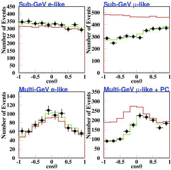
Figure 1: Zenith angle distribution of Super-Kamiokande sub-GeV and multi-GeV electron and muon events. The black histogram shows the Monte Carlo prediction (under the assumption of no neutrino oscillations). The gray histogram was obtained for $\nu_{\mu}\to\nu_{\tau}$ oscillations with the best-fit values $\Delta m^{2}=2.5\times 10^{-3}\,\mathrm{eV}^{2}$ and $\sin^{2}2\vartheta=1.0$. Figure taken from Ref. [59].

The compelling evidence in favour of neutrino oscillations has been obtained recently by the S-K collaboration [29], from the observation of the large up-down asymmetry of the atmospheric high energy muon events. In the S-K experiment [29] the zenith angle dependence of the numbers of electron and muon events was measured. In the absence of neutrino oscillations, the number of the electron (muon) events in the multi-GeV region must obey the following relation:

$$N_{l}(\cos\theta_{z})=N_{l}(-\cos\theta_{z})\,~{}~{}(l=e,\mu)\,,$$ (120)

where $\theta_{z}$ is the zenith angle.

The results of the S-K experiment on the measurement of the zenith-angle distribution of the atmospheric neutrino events is shown in Fig. 1. As it is seen from this figure, for the electron events there is a good agreement between the data and relation (120). Instead, for the Multi-GeV muon events a significant violation of relation (120) was observed. The ratio of the number of up-going muons ($-1\leq\cos\theta_{z}\leq-0.2$) to the number of down-going muons ($0.2\leq\cos\theta_{z}\leq 1$) was found to be

$$\left(\frac{U}{D}\right)_{\mu}=0.54\pm 0.04\pm 0.01.$$

At high energies the direction of leptons practically coincides with the direction of neutrinos. The up-going muons are produced by neutrinos which travel distances from $\simeq 500\,\rm{km}$ to $\simeq 13000\,\rm{km}$ and the down-going muons are produced by neutrinos which travel distances from $\simeq 20\,\rm{km}$ to $\simeq 500\,\rm{km}$. Hence the observation of the up-down asymmetry clearly demonstrates the dependence of the number of muon neutrinos on the distance which they travel from the production point in the atmosphere to the detector.

The S-K data [29] and the data of the other atmospheric neutrino experiments, SOUDAN 2 [30] and MACRO [31], are perfectly described if we assume that the two-neutrino $\nu_{\mu}\to\nu_{\tau}$ oscillations take place. From the analysis of the S-K data it was found [29] that at 90 % $\rm{CL}$ the neutrino oscillation parameters $\Delta m^{2}_{atm}$ and $\sin^{2}2\theta_{atm}$ are in the range

$$1.6\cdot 10^{-3}\leq\Delta m^{2}_{atm}\leq 3.9\cdot 10^{-3}\,~{}\rm{eV}^{2};\,~{}\sin^{2}2\theta_{atm}>0.92;\,,$$

the best-fit values of the parameters being equal to

$$\Delta m^{2}_{atm}=2.5\cdot 10^{-3}\rm{eV}^{2};\,~{}\sin^{2}2\theta_{atm}=1.0\,~{}(\chi^{2}_{\rm{min}}=163.2/170\,\rm{d.o.f.})$$ (121)

7.2 Indications in favour of neutrino oscillations obtained in the K2K experiment

Neutrino oscillations in the atmospheric range of $\Delta m^{2}$ are investigated in the first long baseline accelerator experiment K2K [60]. In this experiment neutrinos, originated mainly from the decay of pions, produced at the 12 GeV KEK accelerator, are recorded by the S-K detector at a distance of about 250 km from the accelerator. The average neutrino energy is $\simeq$ 1.3 GeV.

Two near detectors at a distance of about 300 m from the beam-dump target are used in the K2K experiment: a 1 kt water-Cherenkov detector and a fine-grained detector. The total number and spectrum of muon neutrinos, observed in the S-K detector, are compared to the total number and spectrum calculated from the results of the near detectors under the assumption of the absence of neutrino oscillations. For the measurement of the energy of neutrinos in the S-K detector, quasi elastic one-ring events $\nu_{\mu}+n\to\mu^{-}+p$ are selected.

The first results of the K2K experiment were recently published [60]. The total number of muon events observed in the S-K detector is equal to 56: it must be compared with an expected number of events equal to $80.1^{+6.2}_{-5.4}$. The observed number of the one-ring muon events which was used for the calculation of neutrino spectrum is equal to 29, while the expected number of the one-ring events is equal to 44.

Thus, in the long baseline accelerator K2K experiment, indications in favour of the disappearance of the accelerator $\nu_{\mu}$ were obtained. From the maximum likelihood two-neutrino analysis of the data the following best-fit values of the oscillation parameters were found

$$\sin^{2}2\,\theta_{\rm{K2K}}=1:\,~{}\Delta m^{2}_{\rm{K2K}}=2.8\,~{}10^{-3}\,~{}\rm{eV}^{2}.$$ (122)

These values are in agreement with the values of the oscillation parameters found from the analysis of the S-K atmospheric neutrino data (see (121)). The first K2K results were obtained with $4.8\,~{}10^{19}$ protons on target (POT). It is expected that $10^{20}$ POT will be utilized in the experiment.

7.3 Evidence in favour of the transitions of solar $\nu_{e}$ into $\nu_{\mu}$ and $\nu_{\tau}$

The energy of the sun is produced in the reactions of the thermonuclear pp and CNO cycles, in which protons and electrons are converted into Helium and electron neutrinos:

$$4p+2e^{-}\to^{4}\rm{He}+2\nu_{e}.$$

The reactions, which are most important for the solar neutrino experiments, are listed in Table I. From this Table one can see that the largest part of the solar neutrino flux draw up low energy $\rm{pp}$ neutrinos. According to the SSM BP00 [61], the medium energy mono-energetic ${}^{7}\rm{Be}$ neutrinos make up about 10 % of the total flux, while the high energy ${}^{8}\rm{B}$ neutrinos constitute only about $10^{-2}$ % of the total flux. However, the ${}^{8}\rm{B}$ decay is a very important source of the solar neutrinos: in the S-K [35] and SNO [36, 37, 38] experiments, due to the high energy thresholds, practically only neutrinos from ${}^{8}\rm{B}$-decay can be detected. The ${}^{8}\rm{B}$ neutrinos also give the dominant contribution to the event rate measured in the Homestake experiment [32].

Table I

Reaction	Neutrino energy	SSM BP00 flux
$p\,p\to d\,e^{+}\,\nu_{e}$	$\leq 0.42\,\rm{MeV}$	$5.95\cdot 10^{10}\,\rm{cm}^{-2}\,\rm{s}^{-1}$
$e^{-}+^{7}\rm{Be}\to\nu_{e}\,^{7}\rm{Li}$	$0.86\,\rm{MeV}$	$4.77\cdot 10^{9}\,\rm{cm}^{-2}\,\rm{s}^{-1}$
${}^{8}\rm{B}\to^{8}\rm{Be}^{*}\,e^{+}\,\nu_{e}$	$\leq 15\,\rm{MeV}$	$5.05\cdot 10^{6}\,\rm{cm}^{-2}\,\rm{s}^{-1}$

The main sources of the solar neutrinos. The maximum neutrino energies and SSM BP00 [61] fluxes are also given.

The event rates measured in all solar neutrino experiments are significantly smaller than the ones predicted by the Standard Solar models.

In the Homestake experiment [32] solar neutrinos are detected through the observation of the Pontecorvo-Davis reaction $\nu_{e}+^{37}\rm{Cl}\to e^{-}+^{37}\rm{Ar}$, in the GALLEX-GNO [33] and SAGE [34] experiments through the reaction $\nu_{e}+^{71}\rm{Ga}\to e^{-}+^{71}\rm{Ge}$ and in the S-K [35] experiment solar neutrinos are detected via the observation of the process $\nu+e\to\nu+e$.

For the ratio R of the observed and the predicted by SSM BP00 [61] rates the following values were obtained:

$$R=0.34\pm 0.03\,~{}~{}~{}~{}(\mathrm{Homestake})$$

$$R=0.58\pm 0.05\,~{}~{}~{}~{}(\mathrm{GALLEX-GNO})$$

$$R=0.60\pm 0.05\,~{}~{}~{}~{}(\mathrm{SAGE}))$$

$$R=0.465\pm 0.018\,~{}~{}(\mathrm{S-K})\,.$$

If there is neutrino mixing the original solar $\nu_{e}$’s, due to neutrino oscillations or matter MSW transitions, are transfered into another type of neutrinos, which can not be detected in the radiochemical Homestake, GALLEX-GNO and SAGE experiments. In the S-K experiment mainly $\nu_{e}$ are detected: the sensitivity of the experiment to $\nu_{\mu}$ and $\nu_{\tau}$ is about six times smaller than the sensitivity to $\nu_{e}$. Thus, neutrino oscillations or MSW transition in matter provide a natural explanation for the observed depletion of the fluxes of solar $\nu_{e}$.

Recently a strong model independent evidence in favour of the transition of the solar $\nu_{e}$ into $\nu_{\mu}$ and $\nu_{\tau}$ was obtained in the SNO experiment [36, 37, 38]. The detector in the SNO experiment is a heavy water Cherenkov detector (1 kton of $\rm{D}_{2}O$). Neutrinos from the Sun are detected via the observation of the following three reactions:

$$1.~{}~{}{\rm{CC~{}~{}reaction}}~{}~{}~{}~{}~{}~{}~{}~{}~{}~{} \nu_{e}+d\to e^{-}+p+p\,,$$ (123)

$$2.~{}~{}{\rm{NC~{}~{}reaction}}~{}~{}~{}~{}~{}~{}~{}~{}~{}~{} \nu+d\to\nu+n+p\,,$$ (124)

$$3.~{}~{}{\rm{ES~{}~{}process}}~{}~{}~{}~{}~{}~{}~{}~{}~{}~{} \nu+e\to\nu+e\,$$ (125)

During 306.4 days of running $1967^{+61.9}_{-60.9}$ CC events, $576.5^{+49.5}_{-48.9}$ NC events, and $263.6^{+26.4}_{-25.6}$ ES events were recorded in the SNO experiment. The kinetic energy threshold for the detection of electrons was equal to 5 MeV, the NC threshold to 2.2 MeV. Thus, practically only neutrinos from the decay ${}^{8}\rm{B}\to^{8}\rm{Be}+e^{+}+\nu_{e}$ are detected in the SNO experiment. The important point is that the initial spectrum of ${}^{8}\rm{B}$ neutrinos is known [62].

The total CC event rate can be presented in the form

$$R_{\nu_{e}}^{CC}=<\sigma^{CC}_{\nu_{e}d}>\Phi_{\nu_{e}}^{CC}\,,$$ (126)

where $<\sigma^{CC}_{\nu_{e}d}>$ is the cross section of the CC process (123), averaged over the initial spectrum of ${}^{8}\rm{B}$ neutrinos, and $\Phi_{\nu_{e}}^{CC}$ is the flux of $\nu_{e}$ on the Earth, which is given by the relation

$$\Phi_{\nu_{e}}^{CC}=<P(\nu_{e}\to\nu_{e})>_{CC}\,~{}\Phi_{\nu_{e}}^{0}\,,$$ (127)

where $\Phi_{\nu_{e}}^{0}$ is the total initial flux of $\nu_{e}$ and $<P(\nu_{e}\to\nu_{e})>_{CC}$ is the averaged $\nu_{e}$ survival probability.

All flavour neutrinos $\nu_{e}$, $\nu_{\mu}$ and $\nu_{\tau}$ are recorded via the detection of the NC process (124). Taking into account the $\nu_{e}-\nu_{\mu}-\nu_{\tau}$ universality of the neutral current interaction, for the total NC event rate we have

$$R^{NC}_{\nu}=<\sigma^{NC}_{\nu d}>\Phi_{\nu}^{NC}\,,$$ (128)

where $<\sigma^{NC}_{\nu d}>$ is the cross section of the NC process (124), averaged over the initial spectrum of the ${}^{8}\rm{B}$ neutrinos, and $\Phi_{\nu}^{NC}$ is the total flux of all flavour neutrinos on the Earth. We have

$$\Phi_{\nu}^{NC}=\sum_{l=e,\mu,\tau}\Phi_{\nu_{l}}^{NC}\,,$$ (129)

where

$$\Phi_{\nu_{l}}^{NC}=<P(\nu_{e}\to\nu_{l})>_{NC}\,~{}\Phi_{\nu_{e}}^{0}\,,$$ (130)

$<P(\nu_{e}\to\nu_{l})>_{NC}$ being the averaged probability of the transition $\nu_{e}\to\nu_{l}$ ($l=e,\mu,\tau$).

All flavour neutrinos are detected also via the observation of the ES process (125). However, the cross section of the NC process $\nu_{\mu,\tau}+e\to\nu_{\mu,\tau}+e$ is about six times smaller than the cross section of the CC and NC process $\nu_{e}+e\to\nu_{e}+e$.

The total ES event rate can be presented in the form

$$R^{ES}_{\nu}=<\sigma_{\nu_{e}e}>\Phi_{\nu}^{ES}.$$ (131)

Here $<\sigma_{\nu_{e}e}>$ is the cross section of the process $\nu_{e}e\to\nu_{e}e$, averaged over initial spectrum of the ${}^{8}B$ neutrinos,

$$\Phi_{\nu}^{ES}=\Phi_{\nu_{e}}^{ES}+\frac{<\sigma_{\nu_{\mu}e}>}{<\sigma_{\nu_{e}e}>}\,~{}\Phi_{\nu_{\mu,\tau}}^{ES}\,,$$ (132)

where $\Phi_{\nu_{e}}^{ES}$ ( $\Phi_{\nu_{\mu,\tau}}^{ES}$) is the flux of $\nu_{e}$ ($\nu_{\mu}$ and $\nu_{\tau}$) and

$$\frac{<\sigma_{\nu_{\mu}e}>}{<\sigma_{\nu_{e}e}>}\simeq 0.154.$$ (133)

We have

$$\Phi_{\nu_{l}}^{ES}=<P(\nu_{e}\to\nu_{l})>_{ES}\,~{}\Phi_{\nu_{e}}^{0},$$ (134)

where $<P(\nu_{e}\to\nu_{l})>_{ES}$ is the averaged probability of the transition $\nu_{e}\to\nu_{l}$.

In the SNO experiment it was found [38]

$$(\Phi_{\nu}^{ES})_{\rm{SNO}}=({2.39^{+0.24}_{-0.23}~{}\mbox{(stat.)}\pm 0.12~{}\mbox{(syst.)}})\cdot 10^{6}\,~{}\rm{cm}^{-2}\rm{s}^{-1}\,,$$ (135)

This value is in a good agreement with the value of the ES flux, obtained in the Super-Kamiokande experiment.

In the S-K solar neutrino experiment [35] neutrinos are detected via the observation of the ES process. During 1496 days of running a large number $22400\pm 800$ of solar neutrino events with recoil total energy threshold of 5 MeV were recorded. From the data of the S-K experiment the value

$$(\Phi_{\nu}^{ES})_{\rm{S-K}}=({2.35\pm 0.02~{}\mbox{(stat.)}\pm 0.08~{}\mbox{(syst.)}})\cdot 10^{6}\,~{}\rm{cm}^{-2}\rm{s}^{-1}\,.$$ (136)

was obtained.

In the S-K experiment the spectrum of the recoil electrons was measured: no sizable distortion was observed with respect to the spectrum, expected under the assumption of no neutrino oscillations.

The spectrum of electrons, produced in the CC process (123), was measured in the SNO experiment [38]. Also in this experiment no distortion of the electron spectrum was observed.

Thus, the data of the S-K and SNO experiments are compatible with the assumption that in the high-energy ${}^{8}B$ region the probability of solar neutrinos to survive is practically a constant:

$$P(\nu_{e}\to\nu_{e})\simeq\rm{const}.$$ (137)

The constant $\nu_{e}$ survival probability, Eq. (137), implies

$$<P(\nu_{e}\to\nu_{e})>_{CC}\simeq<P(\nu_{e}\to\nu_{e})>_{NC}\simeq<P(\nu_{e}\to\nu_{e})>_{ES}\,.$$

Taking into account these relations, from (127), (130) and (134) in the high energy ${}^{8}B$ region we obtain

$$\Phi_{\nu_{e}}^{CC}\simeq\Phi_{\nu_{e}}^{NC}\simeq\Phi_{\nu_{e}}^{ES}\,.$$ (138)

In the SNO experiment for the flux of $\nu_{e}$ on the Earth it was found

$$(\Phi_{\nu_{e}}^{CC})_{\rm{SNO}}=({1.76^{+0.06}_{-0.05}\mbox{(stat.)}^{+0.09}_{-0.09}~{}\mbox{(syst.)}})\cdot 10^{6}\,~{}\rm{cm}^{-2}\rm{s}^{-1}.$$ (139)

For the flux of all flavour neutrinos $\Phi_{\nu}^{NC}$ from the NC measurement it was obtained the value

$$(\Phi_{\nu}^{NC})_{\rm{SNO}}=({5.09^{+0.44}_{-0.43}\mbox{(stat.)}^{+0.46}_{-0.43}~{}\mbox{(syst.)}})\cdot 10^{6}\,~{}\rm{cm}^{-2}\rm{s}^{-1}\,,$$ (140)

which is about three times larger than the flux of electron neutrinos on the Earth.

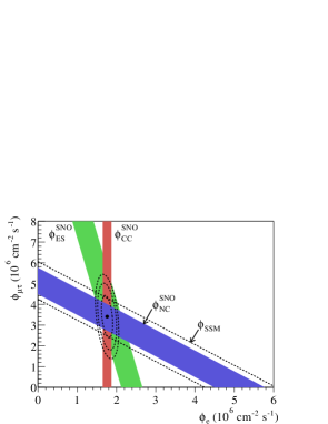
Figure 2: Flux of $\nu_{\mu}$ and $\nu_{\tau}$ vs flux of $\nu_{e}$ in the ⁸B energy region deduced from the three neutrino reactions in SNO. The diagonal bands show the total ⁸B flux as predicted by the BP00 SSM [61] (dashed lines) and that measured in SNO experiment via the observation of NC (solid band). The interception of these bands with the axes represent the $\pm 1\sigma$ errors. The bands intersect at the fit values for $\Phi_{\nu_{e}}$ and $\Phi_{\nu_{\mu,\tau}}$. Figure taken from Ref. [37].

Obviously the NC flux is given by

$$\Phi_{\nu}^{NC}=\Phi_{\nu_{e}}^{NC}+\Phi_{\nu_{\mu,\tau}}^{NC}\,$$ (141)

where $\Phi_{\nu_{e}}^{NC}$ is the flux of $\nu_{e}$ and $\Phi_{\nu_{\mu,\tau}}^{NC}$ is the flux of $\nu_{\mu}$ and $\nu_{\tau}$.

By combining now CC and NC fluxes and using the relation (138), we can determine the flux $\Phi_{\nu_{\mu,\tau}}^{NC}$. In Refs. [38, 37] the ES flux (135) was also taken into account(see Fig. 2). For the flux of $\nu_{\mu}$ and $\nu_{\tau}$ on the Earth the following value

$$(\Phi_{\nu_{\mu,\tau}})_{SNO}=(3.41^{+0.45}_{-0.45}\mbox{(stat.)}^{+0.48}_{-0.45}~{}\mbox{(syst.)})\cdot 10^{6}\,~{}\rm{cm}^{-2}\rm{s}^{-1}$$ (142)

was then obtained. Thus, the detection of solar neutrinos via the simultaneous observation of CC, NC and ES processes allowed the SNO collaboration to obtain a direct model independent $5.3\,~{}\sigma$ evidence of the presence of $\nu_{\mu}$ and $\nu_{\tau}$ in the flux of the solar neutrinos on the Earth.

The total flux of the ${}^{8}B$ neutrinos, predicted by SSM BP00 [61], is equal to

$$(\Phi_{\nu_{e}}^{0})_{\rm{SSM\,BP}}=(5.05^{+1.01}_{-0.81})\cdot 10^{6}\,~{}\rm{cm}^{-2}\rm{s}^{-1}\,.$$ (143)

This value is compatible with the value of total flux of all flavour neutrinos (140), determined from the data of the SNO experiment.

The flux of $\nu_{\mu}$ and $\nu_{\tau}$ on the Earth can be also obtained from the SNO CC data and the S-K ES data. In the first SNO publication [36] the value

$$(\Phi_{\nu_{\mu,\tau}})_{\rm{S-K,SNO}}=(3.69\pm 1.13)\cdot 10^{6}\,~{}\rm{cm}^{-2}\rm{s}^{-1}\,,$$ (144)

was found, which is in a good agreement with the value (142).

The data of all solar neutrino experiments can be described if one assumes that there are transitions of solar $\nu_{e}$ into $\nu_{\mu}$ and $\nu_{\tau}$ and that the $\nu_{e}$ survival probability is given by the two-neutrino expression, which is characterized by two oscillation parameters, $\Delta m^{2}_{\rm{sol}}$ and $\tan^{2}\theta_{\rm{sol}}$. From the global $\chi^{2}$ fit of the total event rates, measured in all solar neutrino experiments, several allowed regions (solutions) in the plane of the oscillation parameters were obtained (see, for example, Ref. [63]): LMA, LOW, SMA, VO and other regions. The situation changed after the recoil electron spectrum was measured in the S-K experiment [35] and the SNO results [36, 38, 37] were obtained. Analyzes of all solar neutrino data showed that the large mixing angle LMA MSW region is the most plausible one (see [64] and references therein). In Ref. [38] the following best-fit LMA values of the solar neutrino oscillation parameters were found:

$$\Delta m^{2}_{\rm{sol}}=5\cdot 10^{-5}\rm{eV}^{2};\,\tan^{2}\theta_{\rm{sol}}=0.34;\,~{}\chi^{2}_{\rm{min}}=57/72\,\rm{d.o.f.}.$$ (145)

Recent data of the KamLAND experiment [39] (see below) allow to exclude all solutions of the solar neutrino problem, except the LMA one.

7.4 Reactor experiments CHOOZ and Palo Verde

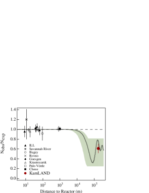
Figure 3: The ratio of measured to expected numbers of $\bar{\nu}_{e}$ events for different reactor neutrino experiments. The shaded region indicates the range of the predictions corresponding to the 95% C.L. LMA region found from the global analysis of the solar neutrino data [65]. The dotted curve corresponds to the best-fit values $\Delta{m}^{2}_{\mathrm{sol}}=5.5\times 10^{-5}\,\mathrm{eV}^{2}$ and $\sin^{2}2\vartheta_{\mathrm{sol}}=0.83$ found in Ref. [65]. Figure taken from Ref. [39].

In the long baseline reactor experiments CHOOZ [41] and Palo Verde [42] the disappearance of the reactor $\bar{\nu}_{e}$’s in the atmospheric range of $\Delta m^{2}$ was searched for. In spite of the fact that in these experiments no indication in favour of neutrino oscillations were found, their results are very important for the neutrino mixing.

In the CHOOZ experiment $\bar{\nu}_{e}$’s from two reactors at a distance of about 1 km from the detector were recorded via the observation of the process

$$\bar{\nu}_{e}+p\to e^{+}+n.$$

The value of the ratio $R$ of the total number of the detected $\bar{\nu}_{e}$ events to the expected number was found to be

$$R=1.01\pm 2.8\%\,(\rm{stat})\pm\pm 2.7\%\,(\rm{syst})\,~{}~{}(\rm{CHOOZ})$$

In the similar Palo Verde experiment it was obtained:

$$R=1.01\pm 2.4\%\,(\rm{stat})\pm 5.3\%\,(\rm{syst})\,~{}~{}(\rm{PaloVerde})$$

The data of the experiments were analyzed in [41, 42] in the framework of two-neutrino oscillations and exclusion plots in the plane of the oscillation parameters $\Delta m^{2}$ and $\sin^{2}2\,\theta$ were obtained. From the CHOOZ exclusion plot at $\Delta m^{2}=2.5\cdot 10^{-3}\,~{}\rm{eV}^{2}$ (the S-K best-fit value) one gets

$$(\sin^{2}2\,\theta)_{\rm{CHOOZ}}\lesssim 1.5\cdot 10^{-1}.$$

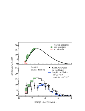
Figure 4: Upper panel: Expected reactor $\bar{\nu}_{e}$ energy spectrum with contributions of $\bar{\nu}_{\mathrm{geo}}$ (antineutrinos produced in ²³⁸U and ²³²Th decays in the Earth) and accidental background. Lower panel: Energy spectrum of the observed prompt events (solid circles with error bars), along with the expected no oscillation spectrum (upper histogram, with $\bar{\nu}_{\mathrm{geo}}$ and accidentals shown) and best fit (lower histogram) in the case of neutrino oscillations. The shaded band indicates the systematic error in the best-fit spectrum. The vertical dashed line corresponds to the threshold of 2.6 MeV. Figure is taken from Ref. [39].

7.5 The KamLAND evidence in favour of the disappearance of the reactor $\bar{\nu}_{e}$

The first results of the KamLAND experiment [39] were published recently. In this experiment $\bar{\nu}_{e}$’s from many reactors in Japan and Korea are detected via the observation of the classical process

$$\bar{\nu}_{e}+p\to e^{+}+n$$

The threshold of this process is $\simeq$ 1.8 MeV. About 80 % of the total number of the events is due to $\bar{\nu}_{e}$ from 26 reactors within the distances of 138-214 km.

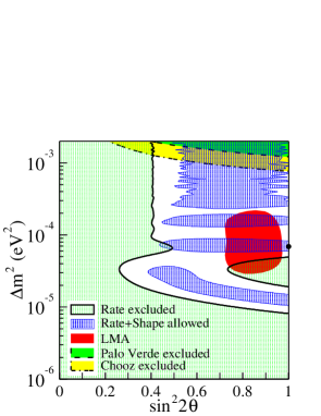
Figure 5: KamLAND excluded regions of neutrino oscillation parameters $\Delta m^{2}$ and $\sin^{2}2\theta$ for the rate analysis and allowed regions for the combined rate and energy spectrum analysis at 95% C.L. At the top are the 95% C.L. excluded region from CHOOZ [41] and Palo Verde [42] experiments, respectively. The dark area is the 95% C.L. LMA allowed region obtained in Ref. [65]. The thick dot indicates the best-fit values of the oscillation parameters. Figure taken from Ref. [39].

The 1 kt liquid scintillator detector of the KamLAND experiment is located in the Kamioka mine at a depth of about 1 km. Both prompt photons from the annihilation of $e^{+}$ in the scintillator and 2.2 MeV delayed photons from the neutron capture $n+p\to d+\gamma$ are detected. The mean neutron capture time is $188\pm 23\,\mu$sec. In order to avoid background, mainly from the the decay of ${}^{238}\rm{U}$ and ${}^{232}\rm{Th}$ in the Earth, the cut $E_{prompt}>2.6\,\rm{MeV}$ was applied.

During 145.1 days of running there were observed 54 $\bar{\nu}_{e}$ events. The number of the events expected in the absence of neutrino oscillations is equal to $86.8\pm 5.6$. For the ratio of observed and expected $\bar{\nu}_{e}$ events the following value

$$\frac{N_{obs}-N_{BG}}{N_{exp}}=0.611\pm 0.085\pm 0.041.$$ (146)

was obtained.

In Fig. 3, for all reactor neutrino experiments, the dependence of the ratio of the observed and expected $\bar{\nu}_{e}$ events on the average distance between reactors and detectors is plotted. The dotted curve was calculated with the best-fit solar neutrino LMA values of the oscillation parameters $\Delta m^{2}=5.5\cdot 10^{-5}\rm{eV}^{2}$ and $\sin^{2}2\,\theta=0.83$, obtained in Ref. [65].

In the KamLAND experiment the prompt energy spectrum was also measured (see Fig. 4). The prompt energy is connected with the energy of $\bar{\nu}_{e}$ by the relation $E_{prompt}=E_{\bar{\nu}_{e}}-0.8\,\rm{MeV}-\bar{E_{n}}$ ($\bar{E_{n}}$ being the average energy of the neutron). From the two-neutrino analysis of the KamLAND data the following best-fit values of the oscillation parameters were obtained

$$(\Delta m^{2})_{\rm{KamLAND}}=6.9\cdot 10^{-5}\rm{eV}^{2};\,~{}(\sin^{2}2\,\theta)_{\rm{KamLAND}}=1\,.$$

These values are compatible with the values of the oscillation parameters in the solar neutrino LMA MSW region. The allowed region in the plane of the oscillation parameters, obtained from the analysis of the measured rate and measured spectrum is shown in Fig. 5 (95 % CL). The region outside the solid line is excluded from the rate analysis. The dark region is the solar neutrino LMA allowed region, obtained in Ref. [65].

The KamLAND results provide a strong evidence for neutrino masses and oscillations, obtained for the first time in an experiment with terrestrial antineutrinos with the expected flux well under control. It allows us to exclude the SMA, LOW and VAC regions of neutrino oscillation parameters. The only viable solution of the solar neutrino problem appears to be the LMA MSW solution.

8 Neutrino oscillations in the framework of three-neutrino mixing

8.1 Neutrino oscillations in the atmospheric range of the neutrino mass-squared difference

We have discussed evidences in favour of neutrino oscillations, which were obtained in the solar, atmospheric and reactor KamLAND neutrino experiments. At present there exists also an indication in favour of the transition $\bar{\nu}_{\mu}\to\bar{\nu}_{e}$, that was obtained in the single accelerator LSND experiment [66]. The LSND data can be explained by neutrino oscillations. From the analysis of the data, the following ranges for the values of the oscillation parameters

$$2\cdot 10^{-1}\lesssim(\Delta m^{2})_{\rm{LSND}}\lesssim 1\,\rm{eV}^{2};$$

$$3\cdot 10^{-3}\lesssim(\sin^{2}2\,\theta)_{\rm{LSND}}\lesssim 4\cdot 10^{-2}$$

were obtained.

In order to describe the data of the solar, atmospheric, KamLAND and LSND experiments, which require three different values of neutrino mass-squared differences, it is necessary to assume that there are (at least) four massive and mixed neutrinos. This means that in addition to the three flavour neutrinos (at least) one sterile neutrino must exist (see, for example, Ref. [45]). The result of the LSND experiment requires, however, confirmation. The MiniBooNE experiment at Fermilab [67], which started in 2002, is aimed at checking the LSND result.

We will consider here the minimal scheme of three-neutrino mixing

$$\nu_{\alpha L}=\sum_{i=1}^{3}\,U_{\alpha i}\,\nu_{iL},$$ (147)

where $U$ is the unitary 3$\times$3 PMNS mixing matrix. This scheme provides two independent $\Delta m^{2}$’s and allows us to describe solar, atmospheric, KamLAND and other neutrino oscillation data.

Let us start with the consideration of neutrino oscillations in the atmospheric range of $\Delta m^{2}$, which can be explored in the atmospheric and long baseline accelerator and reactor neutrino experiments. In the framework of the three-neutrino mixing (147), with $m_{1}<m_{2}<m_{3}$, there are two possibilities:

I. Hierarchy of neutrino mass-squared differences

$$\Delta m^{2}_{21}\simeq\Delta m^{2}_{\rm{sol}};\,\Delta m^{2}_{32}\simeq\Delta m^{2}_{\rm{atm}};\,~{}\Delta m^{2}_{21}\ll\Delta m^{2}_{32}.$$ (148)

II. Inverted hierarchy of neutrino mass-squared differences

$$\Delta m^{2}_{32}\simeq\Delta m^{2}_{\rm{sol}};\,\Delta m^{2}_{21}\simeq\Delta m^{2}_{\rm{atm}};\,~{}\Delta m^{2}_{32}\ll\Delta m^{2}_{21}.$$ (149)

We will first assume that the neutrino mass spectrum is of the type I. The values of ${L}/{E}$, relevant for neutrino oscillations in the atmospheric range of neutrino mass-squared difference, satisfy the inequality:

$$\Delta m^{2}_{21}\,~{}\frac{L}{E}\ll 1.$$

Thus, we can neglect the contribution of $\Delta m^{2}_{21}$ to the transition probability, Eq. (58). In this case, for the probability of the transition $\nu_{\alpha}\to\nu_{\alpha^{\prime}}$ we obtain the following expression

$${\mathrm{P}}(\nu_{\alpha}\to\nu_{\alpha^{\prime}})\simeq\left|\delta_{{\alpha^{\prime}}\alpha}+U_{\alpha^{\prime}3}U_{\alpha 3}^{*}\,~{}(e^{-i\Delta m^{2}_{32}\frac{L}{2E}}-1)\right|^{2}\,.$$ (150)

Hence, in the leading approximation, the transition probabilities in the atmospheric range of $\Delta m^{2}$ are determined by the largest neutrino mass-squared difference $\Delta m^{2}_{32}$ and by the elements of the third column of the neutrino mixing matrix, which connect the flavour neutrino fields $\nu_{\alpha L}$ with the field of the heaviest neutrino $\nu_{3L}$.

For the appearance probability we obtain from Eq. (150) the expression

$${\mathrm{P}}(\nu_{\alpha}\to\nu_{\alpha^{\prime}})=\frac{1}{2}{\mathrm{A}}_{{\alpha^{\prime}};\alpha}\left(1-\cos\Delta m^{2}_{32}\,\frac{L}{2E}\right)\,~{}(\alpha\not=\alpha^{\prime}),$$ (151)

where the oscillation amplitude is given by

$${\mathrm{A}}_{{\alpha^{\prime}};\alpha}=4\,~{}|U_{\alpha^{\prime}3}|^{2}\,~{}|U_{\alpha 3}|^{2}\,.$$ (152)

The survival probability can be obtained from the condition of conservation of probability and from Eqs. (151) and  (151 we have

$${\mathrm{P}}(\nu_{\alpha}\to\nu_{\alpha})=1-\sum_{\alpha^{\prime}\not=\alpha}\,{\mathrm{P}}(\nu_{\alpha}\to\nu_{\alpha^{\prime}})=1-\frac{1}{2}{\mathrm{B}}_{\alpha;\alpha}\left(1-\cos\Delta m^{2}_{32}\,\frac{L}{2E}\right)\,.$$ (153)

Taking into account the unitarity of the mixing matrix, the amplitude ${\mathrm{B}}_{\alpha;\alpha}$ can be written as:

$${\mathrm{B}}_{\alpha;\alpha}\equiv\sum_{\alpha^{\prime}\not=\alpha}\,{\mathrm{A}}_{{\alpha^{\prime}};\alpha}=4\,|U_{\alpha 3}|^{2}\,\left(1-|U_{\alpha 3}|^{2}\right)\,.$$ (154)

Obviously, in the case of inverted hierarchy of the neutrino mass-squared differences (case II above) the transition probabilities can be obtained from Eqs. (151)-(154) with the replacements $\Delta m^{2}_{32}\to\Delta m^{2}_{21}$ and $|U_{\alpha 3}|^{2}\to|U_{\alpha 1}|^{2}$.

We notice that the transition probability (151) depends only on $|U_{\alpha 3}|^{2}$ and $\Delta m^{2}_{32}$. The CP phase does not enter into this equation and in the leading approximation the relation

$${\mathrm{P}}(\nu_{\alpha}\to\nu_{\alpha^{\prime}})={\mathrm{P}}(\bar{\nu}_{\alpha}\to\bar{\nu}_{\alpha^{\prime}})$$ (155)

is automatically satisfied.

Thus, the investigation of the effects of CP violation in the lepton sector in the future long baseline neutrino oscillation experiments will be a difficult problem: possible effects are suppressed due to the smallness of the parameter ${\Delta m^{2}_{12}}/{\Delta m^{2}_{32}}$. High precision experiments on the search for effects of CP-violation in the lepton sector are planned for the future neutrino facility JHF [68] and Neutrino Factories [69, 70].

The transition probabilities (151) and (153) have a two-neutrino form in each channel. This is the obvious consequence of the fact that only the largest mass-squared difference $\Delta{m}^{2}_{32}$ contributes to the transition probabilities. The elements $|U_{\alpha 3}|^{2}$, which determine the oscillation amplitudes, satisfy the unitarity condition $\sum_{\alpha}|U_{\alpha 3}|^{2}=1$. Hence, in leading approximation, transition probabilities are characterized by three parameters. We can choose the latter to be:

$$\Delta m^{2}_{32},\,\,\,~{}\sin^{2}\theta_{23},\,\,\,~{}|U_{e3}|^{2}$$

Then, from Eqs. (70) and (152), for the amplitudes of $\nu_{\mu}\to\nu_{\tau}$ and $\nu_{\mu}\to\nu_{e}$ transitions we obtain the expressions

$$A_{\tau;\mu}=(1-|U_{e3}|^{2})^{2}\sin^{2}2\,\theta_{23};\,~{}$$

$$A_{e;\mu}=4\,|U_{e3}|^{2}\,(1-|U_{e3}|^{2}\sin^{2}\,\theta_{23}\,.$$

8.2 Oscillations in the solar range of neutrino mass-squared difference

Let us consider now, in the framework of the tree-neutrino mixing, neutrino oscillations in the solar range of $\Delta m^{2}$. The $\nu_{e}$ survival probability in vacuum can be written in the form

$${\mathrm{P}}(\nu_{e}\to\nu_{e})=\left|\sum_{i=1,2}|U_{ei}|^{2}\,e^{-i\,\Delta{m}^{2}_{i1}\frac{L}{2E}}+|U_{e3}|^{2}\,e^{-i\,\Delta{m}^{2}_{31}\frac{L}{2E}}\,\right|^{2}$$ (156)

We are interested in the $\nu_{e}$ survival probability averaged over the region where neutrinos are produced, over energy resolution etc. Because of the hierarchy $\Delta m^{2}_{32}\gg\Delta m^{2}_{21}$, in the expression for the averaged survival probability the interference between the first and the second terms in Eq. (156) disappears. The averaged survival probability can then be presented in the form

$${\mathrm{P}}(\nu_{e}\to\nu_{e})=|U_{e3}|^{4}+\left(1-|U_{e3}|^{2}\right)^{2}\,~{}P^{(1,2)}(\nu_{e}\to\nu_{e})\,.$$ (157)

Here $P^{(1,2)}(\nu_{e}\to\nu_{e})$ is given by the expression

$${\mathrm{P}}^{(1,2)}(\nu_{e}\to\nu_{e})=1-\frac{1}{2}\,~{}A^{(1,2)}\,~{}\left(1-\cos\Delta m^{2}_{21}\frac{L}{2E}\right)\,,$$ (158)

where

$$A^{(1,2)}=4\,\frac{|U_{e1}|^{2}\,|U_{e2}|^{2}}{(1-|U_{e3}|^{2})^{2}}.$$ (159)

With the help of Eq. (61), Eq. (159) simplifies to

$$A^{(1,2)}=\sin^{2}2\,\theta_{12}\,.$$ (160)

Thus, the probability ${\mathrm{P}}^{(1,2)}(\nu_{e}\to\nu_{e})$ is again characterized by two parameters only and has the standard two-neutrino form.

The expression (157) is also valid for oscillations in matter (see [71, 45]). In this case $P^{(1,2)}(\nu_{e}\to\nu_{e})$ is the two-neutrino $\nu_{e}$ survival probability in matter, calculated under the condition that the density of electrons $\rho_{e}(x)$ in the effective Hamiltonian of the interaction of neutrino with matter is changed by $(1-|U_{e3}|^{2})\,\rho_{e}(x)$.

Hence, the $\nu_{e}$ survival probability is characterized, in the solar range of $\Delta m^{2}$, by three parameters

$$\Delta m^{2}_{21},\,\,\,~{}\tan^{2}\theta_{12},\,\,\,~{}|U_{e3}|^{2}.$$

The only common parameter for the atmospheric and solar ranges of $\Delta m^{2}$ is $|U_{e3}|^{2}$. As we will see in the next subsection, from the data of the reactor CHOOZ and Palo Verde experiments, this parameter turns out to be small.

8.3 The upper bound of $|U_{e3}|^{2}$ from the CHOOZ data. Decoupling of oscillations in the solar and atmospheric ranges of $\Delta m^{2}$

The long baseline reactor experiments CHOOZ [41] and Palo Verde [42] are sensitive to the atmospheric range of $\Delta m^{2}$. No indications in favour of the disappearance of reactor $\bar{\nu}_{e}$ was obtained in these experiments. From the analysis of their data a stringent bound on the parameter $|U_{e3}|^{2}$ was obtained, as it is explained below.

In the framework of the three-neutrino mixing the probability of $\bar{\nu}_{e}$ to survive in the atmospheric range of $\Delta m^{2}$ is given by the expression

$${\mathrm{P}}(\bar{\nu}_{e}\to\bar{\nu}_{e})=1-\frac{1}{2}{\mathrm{B}}_{e;e}\,~{}\left(1-\cos\Delta m^{2}_{32}\frac{L}{2E}\right)\,,$$ (161)

where

$${\mathrm{B}}_{e;e}=4\,|U_{e3}|^{2}\,\left(1-|U_{e3}|^{2}\right)\,.$$ (162)

In Refs. [41, 42] exclusion plots in the plane of the parameters $\Delta m^{2}\equiv\Delta m^{2}_{32}$ and $\sin^{2}2\theta\equiv{\mathrm{B}}_{e;e}$ were obtained, from which one has

$${\mathrm{B}}_{e;e}\leq{\mathrm{B}}_{e;e}^{0},$$ (163)

where the upper bound ${\mathrm{B}}_{e;e}^{0}$ depends on $\Delta m^{2}_{32}$. For the S-K allowed values of the parameter $\Delta m^{2}_{32}$, from the CHOOZ exclusion plot we have

$$1\cdot 10^{-1}\leq{\mathrm{B}}_{e;e}^{0}\leq 2.4\cdot 10^{-1}.$$ (164)

From Eqs. (162) and (164) the following bounds on the parameter $|U_{e3}|^{2}$ can be easily obtained:

$$|U_{e3}|^{2}\leq\frac{1}{2}\,\left(1-\sqrt{1-{\mathrm{B}}_{e;e}^{0}}\right)\lesssim\frac{1}{4}\,{\mathrm{B}}_{e;e}^{0}$$ (165)

or

$$|U_{e3}|^{2}\gtrsim\frac{1}{2}\,\left(1+\sqrt{1-{\mathrm{B}}_{e;e}^{0}}\right)\geq 1-\frac{1}{4}\,{\mathrm{B}}_{e;e}^{0}\,.$$ (166)

Thus, the parameter $|U_{e3}|^{2}$ can be either small or large (close to one). This last possibility is excluded, however, by the solar neutrino data. In fact, if $|U_{e3}|^{2}$ is large, from Eq. (157) it follows that in the whole range of the solar neutrino energies the probability of $\nu_{e}$ to survive is close to one in obvious contradiction with the solar neutrino data. Hence, the upper bound of the parameter $|U_{e3}|^{2}$ is given by Eq. (165). At the S-K best-fit value $\Delta m^{2}_{32}=2.5\cdot 10^{-3}\rm{eV}^{2}$ we get:

$$|U_{e3}|^{2}\leq 4\cdot 10^{-2}\,~{}(95\%\,~{}\rm{CL}).$$ (167)

Taking into account the accuracies of the present-day experiments, one can neglect $|U_{e3}|^{2}$ in the expressions for the transition probabilities. In this approximation, neutrino oscillations in the atmospheric range of $\Delta m^{2}$ are $\nu_{\mu}\to\nu_{\tau}$ oscillations, with $\Delta m^{2}_{32}\simeq\Delta m^{2}_{\rm{atm}}$ and $A_{\tau;\mu}\simeq\sin^{2}2\,\theta_{23}\simeq\sin^{2}2\,\theta_{\rm{atm}}$. In the solar range of $\Delta m^{2}$ we have

$${\mathrm{P}}(\nu_{e}\to\nu_{e})\simeq{\mathrm{P}}^{(1,2)}(\nu_{e}\to\nu_{e}),$$ (168)

where the two-neutrino survival probability ${\mathrm{P}}(\nu_{e}\to\nu_{e})$ depends on the parameters $\Delta m^{2}_{21}\simeq\Delta m^{2}_{\rm{sol}}$ and $\tan^{2}2\,\theta_{12}\simeq\tan^{2}2\,\theta_{\rm{sol}}$.

Thus, due to the smallness of the parameter $|U_{e3}|^{2}$ and the hierarchy of neutrino mass squared differences $\Delta m^{2}_{12}\ll\Delta m^{2}_{32}$ neutrino oscillations in the atmospheric and solar ranges of $\Delta m^{2}$, in the leading approximation, are decoupled [72, 45] and are described by the two-neutrino formulas, which are characterized, respectively, by the oscillation parameters

$$\Delta m^{2}_{32},\,~{}~{}\sin^{2}2\,\theta_{23}\,\,~{}~{}~{}\rm{and}\,\,~{}~{}~{}\Delta m^{2}_{21},\,~{}~{}\tan^{2}\theta_{12}$$

. From the CHOOZ data only the upper bound of the parameter $|U_{e3}|^{2}$ can be obtained. The possibilities to investigate effects of the three-neutrino mixing and in particular important effects of CP violation in the lepton sector depend on the value of this parameter. The value of the parameter $|U_{e3}|^{2}$ will be probed in MINOS [73] and ICARUS [74] experiments and in neutrino experiments at JHF [75] and Neutrino Factories (see [69, 70]).

From the data of the experiments on the investigation of neutrino oscillations only neutrino mass-squared differences $\Delta m^{2}_{21}$ and $\Delta m^{2}_{32}$ can be determined. Neutrino masses $m_{2}$ and $m_{3}$ are given by the relations

$$m_{2}=\sqrt{m^{2}_{1}+\Delta m^{2}_{21}};\,~{}m_{3}=\sqrt{m^{2}_{1}+\Delta m^{2}_{32}+\Delta m^{2}_{21}}\,.$$ (169)

In the next section we will discuss the results of experiments which allow us to obtain information about the absolute values of neutrino masses.

9 $\beta$-decay experiments on the measurement of neutrino mass

The standard method for the measurement of the absolute value of the neutrino mass is based on the detailed investigation of the high-energy part of the $\beta$-spectrum of the decay of tritium

$${}^{3}H\to^{3}He+e^{-}+\bar{\nu}_{e}\,.$$ (170)

This decay is the super-allowed one. Thus, the nuclear matrix element is a constant and the electron spectrum is determined by the phase space. The decay (170) has a small energy release ($E_{0}\simeq 18.6\,~{}\rm{keV}$) and a convenient time of life ($T_{1/2}\simeq 12.3$ years).

The standard effective Hamiltonian of the $\beta$-decay is given by

$$\mathcal{H}_{I}^{\mathrm{CC}}=\frac{G_{F}}{\sqrt{2}}\,2\bar{e}_{L}\gamma_{\alpha}\nu_{eL}\,~{}j^{\alpha}+\mathrm{h.c.}\,.$$ (171)

Here $j^{\alpha}$ is the hadronic charged current, $G_{F}$ is the Fermi constant and

$$\nu_{eL}=\sum_{i}U_{ei}\nu_{iL}\,,$$ (172)

where $\nu_{i}$ is the field of neutrino with mass $m_{i}$ and $U$ is the unitary mixing matrix.

Neglecting the recoil of the final nucleus, from Eqs. (171) and (172) for the spectrum of electrons we obtain the following expression

$$\frac{d\,\Gamma}{d\,E}=\sum_{i}|U_{ei}|^{2}\,~{}\frac{d\,\Gamma_{i}}{d\,E}\,,$$ (173)

where

$$\frac{d\,\Gamma_{i}}{d\,E}=$$ (174)

$$\,\,=C\,p\,(E+m_{e})\,(E_{0}-E)\,\sqrt{(E_{0}-E)^{2}-m_{i}^{2}}\,F(E)\,\theta(E_{0}-E-m_{i})\,,$$

$E$ being the kinetic energy of the electron, $E_{0}$ the energy released in the decay and $m_{e}$ is the mass of the electron. The Fermi function $F(E)$ takes into account the Coulomb interaction of the final particles and the constant $C$ is given by the expression

$$C=G_{F}^{2}\frac{m_{e}^{5}}{2\,\pi^{3}}\,\cos^{2}\,\theta\,_{C}\,|M|^{2}\,,$$

where $\theta\,_{C}$ is the Cabibbo angle and $M$ the nuclear matrix element ( which is a constant).

The sensitivity to the neutrino mass of the present-day tritium experiments Troitsk [76] and Mainz [77] is 2-3 eV. In the future experiment KATRIN [78] a sensitivity of 0.25 eV is expected. Taking into account that $\sqrt{\Delta m^{2}_{\rm{atm}}}\simeq 5\,10^{-2}\,\rm{eV}$ is much smaller than the sensitivities of the present and future tritium experiments, from the relations (169) we can conclude that the neutrino mass can be measured in these experiments only if the neutrino mass spectrum is practically degenerate: $m_{1}\simeq m_{2}\simeq m_{3}$. In this case, from the unitarity of the mixing matrix we have:

$$\frac{d\,\Gamma}{d\,E}=C\,p\,(E+m_{e})\,(E_{0}-E)\,\sqrt{(E_{0}-E)^{2}-m_{1}^{2}}\,~{}F(E)\,.$$ (175)

Let us discuss now the results of the tritium experiments. In the Mainz experiment [77] the target is molecular tritium condensed on a graphite substrate. The spectrum of the electron is measured by the integral electrostatic spectrometer, which combines high luminosity with high resolution. The resolution of the Mainz spectrometer is equal to $4.8\,~{}\rm{eV}$. In the analysis of the experimental data four free variable parameters are used: the normalization $C$, the background $B$, the released energy $E_{0}$ and the neutrino mass-squared $m^{2}_{1}$. The analysis of 1998, 1999 and 2001 data gave the following result:

$$m^{2}_{1}=(-1.2\pm 2.2\pm 2.1)\,~{}\rm{eV}^{2}\,.$$ (176)

This value corresponds to the upper bound

$$m_{1}<2.2\,~{}\rm{eV}\,~{}~{}~{}(95\%\,~{}\rm{CL})\,.$$ (177)

The integral electrostatic spectrometer is also used in the Troitsk neutrino experiment [76]: its resolution is 3.5-4 eV. In the Troitsk experiment the source is a gaseous molecular tritium source. From the four-parameter fit of the Troitsk data, for the parameter $m^{2}_{1}$ large negative values, in the range ($-10\div-20$) eV², were obtained. The investigation of the character of the measured spectrum suggests that the effect of obtaining a negative $m^{2}_{1}$ is due to a step function superimposed on the integral continuous spectrum: the step function in the integral spectrum corresponds to a narrow peak in the differential spectrum.

In the analysis of the data, the authors of the Troitsk experiment added to the theoretical integral spectrum a step function with two additional variable parameters ( the position of the step $E_{\rm{step}}$ and its height). From the six-parameter fit of the data, the following value for the parameter $m^{2}_{1}$

$$m^{2}_{1}=(-2.3\pm 2.5\pm 2.0)\,~{}\rm{eV}^{2}\,.$$ (178)

was found. From (178) the upper bound on the neutrino mass $m_{1}$

$$m_{1}<2.2\,~{}\rm{eV}\,~{}~{}~{}(95\%\,~{}\rm{CL})\,.$$ (179)

can be deduced.

The analysis of the Troitsk data shows that the position of the step $E_{0}-E_{\rm{step}}$ is periodically changed in the interval 5-15 eV and the average value of the height of the step is about $6\cdot 10^{-11}$. The existence of this anomaly was not confirmed by the Mainz experiment [77].

A new tritium experiment, KATRIN [78], is now under preparation. In this experiment gaseous molecular source and frozen tritium source are planned to be used. The integral electrostatic spectrometer will have two parts: the pre-spectrometer, which will select electrons in the last $\simeq 100$ eV of the spectrum, and the main spectrometer. The latter will have a resolution of $\simeq 1$ eV. It is expected that the KATRIN experiment will start to collect data in 2007. After three years of running the accuracy of the measurement of the neutrino mass will reach $\simeq 0.25$ eV.

In order to understand the origin of the small neutrino masses we need to know the nature of the massive neutrinos: are they Majorana or Dirac particles? As we have seen, neutrino oscillation experiments can not answer this fundamental question. The nature of the massive neutrinos can be revealed in experiments on the search for neutrinoless double $\beta$-decay of some even-even nuclei. The next section will be devoted to the discussion of such experiments.

10 Neutrinoless double $\beta$-decay

The search for neutrinoless double $\beta$-decay

$$(A,Z)\to(A,Z+2)+e^{-}+e^{-}$$ (180)

of some even-even nuclei is the most sensitive and direct way of investigating the nature of neutrinos with definite masses. The total lepton number in the process (180) is violated and this is allowed only if the massive neutrinos $\nu_{i}$ are Majorana particles.

We will assume that the Hamiltonian of the process has the standard form, Eq.(171), and that the flavour field $\nu_{eL}$ is given by

$$\nu_{eL}=\sum_{i}U_{ei}\nu_{iL}\,,$$ (181)

where $\nu_{i}$ are Majorana fields.

The neutrinoless double $\beta$-decay ($(\beta\,\beta)_{0\nu}$ -decay) is a process of second order in the Fermi constant $G_{F}$, with virtual neutrinos. For small neutrino masses the neutrino propagator is given by the expression

$$<0|T(\nu_{eL}(x_{1})\nu^{T}_{eL}(x_{2}))|0>\simeq m_{\beta\beta}\,~{}\frac{i}{(2\,\pi)^{4}}\int\frac{d^{4}p}{p^{2}}\,{e^{-ip(x_{1}-x_{2})}}\,\frac{1-\gamma_{5}}{2}\,C\,,$$ (182)

where

$$m_{\beta\beta}=\sum_{i}U^{2}_{ei}\,m_{i}\,.$$ (183)

The total matrix element of the $(\beta\beta)_{0\nu}$ -decay is a product of $m_{\beta\beta}$ and the nuclear matrix element, which does not depend on neutrino masses and mixing.

Results of many experiments on the search for $(\beta\beta)_{0\nu}$-decay are available at present (see Refs. [79, 80]). No indication in favour of $(\beta\beta)_{0\nu}$-decay was obtained so far. The most stringent lower bounds for the time of life of $(\beta\,\beta)_{0\,\nu}$-decay were obtained in the Heidelberg-Moscow [84] and IGEX [85] ⁷⁶Ge experiments:

$$T^{0\nu}_{1/2}\geq 1.9\cdot 10^{25}\,y\,~{}~{}(90\%\,\rm{CL})\,~{}~{}\rm{Heidelberg-Moscow}$$

$$T^{0\nu}_{1/2}\geq 1.57\cdot 10^{25}\,y\,~{}~{}(90\%\,\rm{CL})\,~{}~{}\rm{IGEX}$$

Taking into account different calculations of the nuclear matrix element, from these results the following upper bounds were obtained for the effective Majorana mass:

$$|m_{\beta\beta}|\leq(0.35-1.24)\,~{}\rm{eV}\,.$$ (184)

Many new experiments on the search for the neutrinoless double $\beta$-decay are in preparation at present (see Ref. [79]). In these experiments the sensitivities

$$|m_{\beta\beta}|\simeq(1\cdot 10^{-1}-1.5\cdot 10^{-2})\,~{}\rm{eV}$$

are expected to be achieved.

The evidence for neutrinoless double $\beta$- decay would be a proof that neutrinos with definite masses are Majorana particles. The value of the effective Majorana mass $|m_{\beta\beta}|$ combined with the values of the neutrino oscillation parameters, obtained from the results of neutrino oscillation experiments, would enable us to obtain important information about the character of the neutrino mass spectrum, the minimal neutrino mass $m_{1}$ and the Majorana CP phase (see Ref. [86] and references therein).

We will consider here three typical neutrino mass spectra.

1. The hierarchy of neutrino masses $m_{1}\ll m_{2}\ll m_{3}$.

   In this case for the effective Majorana mass we have the following upper bound :

   $$|m_{\beta\beta}|\leq\sin^{2}\theta_{\rm{sol}}\,\sqrt{\Delta m^{2}_{\rm{sol}}}+|U_{e3}|^{2}\,\sqrt{\Delta m^{2}_{\rm{atm}}}.$$ (185)

   Using the best-fit values of the oscillation parameters and the CHOOZ limit on $|U_{e3}|^{2}$ (see Eqs. (71), (95) and (167)), we obtain from (185) the upper bound

   $$|<m>|\leq 3.8\cdot 10^{-3}\rm{eV}\,,$$ (186)

   which is significantly smaller than the expected sensitivities of the future $(\beta\beta)_{0\nu}$- experiments.

2. Inverted hierarchy of neutrino masses: $m_{1}\ll m_{2}<m_{3}$.

   The effective Majorana mass is given, in this case, by the expression

   $$|m_{\beta\beta}|\simeq\left(1-\sin^{2}2\,\theta_{\rm{sol}}\,\sin^{2}\alpha\right)^{\frac{1}{2}}\,\sqrt{\Delta m^{2}_{\rm{atm}}},$$ (187)

   where $\alpha=\alpha_{3}-\alpha_{2}$ is the the difference of the Majorana CP phases ($U_{ei}=|U_{ei}|\,~{}e^{i\,\alpha_{i}}$). From this expression it follows that

   $$\sqrt{\Delta m^{2}_{\rm{atm}}}\,~{}|\cos 2\,\theta_{sol}|\lesssim|m_{\beta\beta}|\lesssim\sqrt{\Delta m^{2}_{\rm{atm}}}\,,$$ (188)

   where the upper and lower bounds correspond to the case of CP conservation with equal and opposite CP parities of $\nu_{3}$ and $\nu_{2}$, respectively.

   Using the best-fit value of the parameter $\tan^{2}\theta_{sol}$ (see Eq. (145)), we have

   $$\frac{1}{2}\,\sqrt{\Delta m^{2}_{\rm{atm}}}\lesssim|m_{\beta\beta}|\lesssim\sqrt{\Delta m^{2}_{\rm{atm}}}\,,$$ (189)

   Thus, in the case of the inverted mass hierarchy, the scale of $|m_{\beta\beta}|$ is determined by $\sqrt{\Delta m^{2}_{\rm{atm}}}$. Should the value of $|m_{\beta\beta}|$ be in the range (189), (which can be reached in the future experiments on the search for $(\beta\beta)_{0\nu}$-decay), then we would have an argument in favour of the inverted neutrino mass hierarchy.

3. Practically degenerate neutrino mass spectrum: $m_{2}\simeq m_{3}\simeq m_{1}\gg\sqrt{\Delta m^{2}_{\rm{atm}}}$.

   The effective Majorana mass in this case is given by the expression

   $$|m_{\beta\beta}|\simeq m_{1}\,~{}|\sum_{i=1}^{3}U_{ei}^{2}|.$$ (190)

   Neglecting the small contribution of $|U_{e3}|^{2}$ ( $|U_{e1}|^{2}$ in the case of the inverted hierarchy), for $|m_{\beta\beta}|$ one obtains relations Eqs. (187)-(189) in which $\sqrt{\Delta m^{2}_{\rm{atm}}}$ is replaced by $m_{1}$. Thus, a signature of the degenerate neutrino mass spectrum would be the occurrence of a value $|m_{\beta\beta}|\gg\sqrt{\Delta m^{2}_{\rm{atm}}}$.

   It is obvious that for neutrino mass $m_{1}$ we have the following bound

   $$|m_{\beta\beta}|\leq m_{1}\leq\frac{|m_{\beta\beta}|}{|\cos 2\,\theta_{\rm{sol}}|}\simeq 2\,|m_{\beta\beta}|$$ (191)

   and the parameter $\sin^{2}\alpha$, which characterizes the violation of the CP invariance in the lepton sector [86], is given by the relation

   $$\sin^{2}\alpha\simeq\left(1-\frac{|m_{\beta\beta}|^{2}}{m_{1}^{2}}\right)\,~{}\frac{1}{\sin^{2}2\theta_{\rm{sol}}}\,.$$ (192)

   Thus, if the mass $m_{1}$ is measured in the future experiments and the value of the parameter $\sin^{2}2\theta_{\rm{sol}}$ is determined with high accuracy in the KamLAND [39], BOREXINO [88] and other neutrino experiments, from the results of the future $(\beta\beta)_{0\nu}$ experiments information on the Majorana CP phase can be inferred.

All previous conclusions are based on the assumption that the value of the effective Majorana mass $|m_{\beta\beta}|$ can be obtained from the measurement of the life-time of the $(\beta\beta)_{0\nu}$-decay. However, the determination of the parameter $|m_{\beta\beta}|$ from the experimental data requires the knowledge of the nuclear matrix elements. At present there are large uncertainties in the calculation of these quantities (see, for example, Refs. [89, 90, 91]). Different calculations of the lifetime of the $(\beta\beta)_{0\,\nu}$-decay differ by about one order of magnitude.

In Ref. [92] a method was proposed, which allows one to check the results of the calculations of the $(\beta\beta)_{0\nu}$-decay nuclear matrix elements in a model independent way. This method can be applied if $(\beta\beta)_{0\nu}$-decay of different nuclei is observed.

11 Conclusion

About forty years after the original idea of B. Pontecorvo, compelling evidence in favour of neutrino oscillations were obtained in the S-K [29], SNO [36, 38, 37], KamLAND [39] and other neutrino experiments. These findings opened a new field of research in particle physics and astrophysics: the physics of massive and mixed neutrinos.

From the results of the experiments it follows that neutrino masses are many orders of magnitude smaller than the masses of leptons and quarks. Tiny neutrino masses are a first signature of a new physics, beyond the Standard Model.

There remain many unsolved problems in the physics of massive and mixed neutrinos. The problem concerning $|U_{e3}|^{2}$ is an urgent one: on the value of $|U_{e3}|^{2}$ depends the possibility to study the effects of the three-neutrino mixing and in particular the effects of CP violation in the lepton sector.

Another problem is the one connected with the LSND experiment [66]. If the LSND result will be confirmed by the MiniBOONE experiment [67], this will imply that the number of light neutrinos is more than three and in addition to the three flavour neutrinos sterile neutrino(s) must exist. If, on the contrary, LSND result is refuted, the minimal scheme with three massive and mixed neutrinos will be a plausible possibility.

The problem of the nature of massive neutrinos (Dirac or Majorana?) is the most fundamental one. This problem can be solved by the experiments on the search for neutrinoless double $\beta$-decay. From the existing data the following bound on the effective Majorana mass was found: $|m_{\beta\beta}|\leq(0.3-1.3)$ eV. In future experiments, now in preparation, a significant improvement of the sensitivity is expected.

Due to the interference nature of the neutrino oscillation phenomenon and to the possibilities of exploring large values of ${L}/{E}$, neutrino oscillation experiments are sensitive to very small values of the neutrino mass-squared differences. The determination of the absolute value of the neutrino masses requires the so-called direct measurements and it is a challenging problem. From the data of the tritium experiments the upper bound $m_{1}\leq 2.2\,\rm{MeV}$ was obtained. The future experiment KATRIN [78] is expected to be sensitive to $m_{1}\simeq 0.25$ MeV.

The progress in cosmological measurements, achieved in the last years, allows one to reach $\simeq 1$ eV sensitivity for the sum of the neutrino masses $\sum_{i}m_{i}$. The most stringent bound,

$$\sum_{i}m_{i}<0.71~{}\rm{eV}\,,$$

was recently obtained in Ref. [94]. For a degenerate neutrino mass spectrum this bound implies

$$m_{i}<0.23~{}\rm{eV}\,.$$

In Ref. [94] the 2dF Galaxy Redshift Survey [93] data, recent WMAP high precision data and other cosmological data were used. A significant improvement of this limit is expected with the future Sloan Digital Sky Survey [95], future WMAP and other data.

We have discussed here mainly the phenomenology of neutrino mixing and oscillations, and the most recent experimental data. For models of neutrino masses and mixing we refer the reader to the recent reviews [46, 47, 48].

References

-
[1]
Wu C.S. et al,
“Experimental Test Of Parity Conservation In Beta Decay”
Phys. Rev. 1957, Vol. 105, p. 1413-1414. -
[2]
Landau L.D.,
“On The Conservation Laws For Weak Interactions”
Nucl. Phys. 1957, Vol. 3, p. 127-131. -
[3]
Lee T.D. and Yang C.N.,
“Parity Nonconservation And A Two Component Theory Of The Neutrino”,
Phys. Rev. 1957, Vol. 105, p. 1671-1675. -
[4]
Salam A.,
“On Parity Conservation And Neutrino Mass”,
Nuovo Cimento 1957, Vol. 5, p. 299-301. -
[5]
Pontecorvo B.,
“Mesonium And Antimesonium”,
Zh. Eksp. Teor. Fiz. 1957, Vol. 33, p. 549-551 [Sov. Phys. JETP 1957, Vol. 6, p. 429]. -
[6]
Pontecorvo B.,
“Inverse Beta Processes And Nonconservation Of Lepton Charge,”
Zh. Eksp. Teor. Fiz. 1957, Vol. 34, p. 247 [Sov. Phys. JETP 1958, Vol. 7, p. 172]. -
[7]
Reines F. and Cowan C.,
“Free Anti-Neutrino Absorption Cross-Section. 1: Measurement Of The Free Anti-Neutrino Absorption Cross-Section By Protons,”
Phys. Rev. 1959, Vol. 113, p. 273. -
[8]
Davis R.,
Bull. Am. Phys. Soc. (Washington meeting, 1959). -
[9]
Goldhaber M., Grodzins L. and Sunyar A.W.,
“Helicity Of Neutrinos,”
Phys. Rev. 1958, Vol. 109, p. 1015-1017. -
[10]
Pontecorvo B.,
“Neutrino Experiments And The Question Of Leptonic-Charge Conservation,”
Zh. Eksp. Teor. Fiz. 1967, Vol. 53, p. 1717-1725 [Sov. Phys. JETP 1968, Vol. 26, p. 984-988]. -
[11]
Pontecorvo B.,
Report PD-205, Chalk River Laboratory, 1946. -
[12]
Feynman R.P. and Gell-Mann M.,
“Theory Of The Fermi Interaction,”
Phys. Rev. 1958, Vol. 109, p. 193-198. -
[13]
Sudarshun E.C.G. and Marshak R.,
‘Chirality Invariance And The Universal Fermi Interaction,”
Phys. Rev. 1958, Vol. 109, p. 1860-1862. -
[14]
Danby G., Gaillard J.M., Goulianos K., Lederman L.M.,
Mistry M., Schwartz M. and Steinberger J.,
“Observation Of High-Energy Neutrino Reactions And The Existence Of Two Kinds Of Neutrinos,”
Phys. Rev. Lett. 1962, Vol. 9, p. 36-44. -
[15]
Pontecorvo B. ,
“Electron And Muon Neutrinos,”
Zh. Eksp. Teor. Fiz. 1959, Vol. 37, p. 1751-1757 [Sov. Phys. JETP 1960, Vol. 10, p. 1236-1240]. -
[16]
Zeldovich Ya. B.,
Dokl. Acad. Nauk. USSR, 1952, Vol. 86, p. 505;
Konopinski E.J. and Mahmoud H.,
“The Universal Fermi Interaction,”
Phys. Rev. 1953, Vol. 92, p. 1045-1049. -
[17]
Gribov V.N. and Pontecorvo B.,
“Neutrino Astronomy And Lepton Charge,”
Phys. Lett. 1969, Vol. B 28, p. 493. -
[18]
Bilenky S.M. and Pontecorvo B.,
“Quark-Lepton Analogy And Neutrino Oscillations,”
Phys. Lett. 1976, Vol. B 61, p. 248;
“The Lepton-Quark Analogy And Muonic Charge,”
Yad. Fiz. 1976, Vol. 24, p. 603. -
[19]
Bilenky S.M. and Pontecorvo B.,
“Again On Neutrino Oscillations,”
Lett. Nuovo Cim. 1976, Vol. 17, p. 569. -
[20]
Bilenky S.M. and Pontecorvo B.,
“Lepton Mixing And Neutrino Oscillations,”
Phys. Rept. 1978, Vol. 41, p. 225-261. -
[21]
Maki Z., Nakagava M. and Sakata S.,
“Remarks On The Unified Model Of Elementary Particles,”
Prog. Theor. Phys. 1962, Vol. 28, p. 870. -
[22]
Bahcall J. and Frautschi S.,
“Lepton Non-Conservation And Solar Neutrinos,”
Phys. Lett. 1969, Vol. B 29, p. 623-625. -
[23]
Eliezer S. and Ross D.A.,
“A ’Cabibbo’ Theory For Leptons And The Neutrino Masses,”
Phys. Rev. 1974, Vol. D 10, p. 3088. -
[24]
Fritzsch H. and Minkowski P.,
“Vector - Like Weak Currents, Massive Neutrinos, And Neutrino Beam Oscillations,”
Phys. Lett. 1976, Vol. B 62, p. 72. -
[25]
Eliezer S. and Swift A.,
“Experimental Consequences Of Electron Neutrino - Muon-Neutrino Mixing In Neutrino Beams,”
Nucl. Phys. 1976, Vol. B 105, p. 45. -
[26]
Bilenky S.M. and Pontecorvo B.,
“Oscillations In Neutrino Beams: Status And Possibilities Of Observation,”
Preprint JINR-E2-10032, Dubna, 1976, Invited paper presented at 18th Int. Conf. on High Energy Physics, Tbilisi, USSR, Jul 15-21, 1976 -
[27]
Pontecorvo B.,
“Lepton Charges And Lepton Mixing,”
Preprint JINR-E2-11160, Published in EPS Conf. 1977, Vol. 2, p.1081, Rapporteur talk presented at EPS Conf. on High Energy Physics, Budapest, Jul 4-9, 1977 -
[28]
“Selected scientific works. Recollections on B. Pontecorvo,”
edited by Bilenky S.M., Blokhintseva T.D., Pokrovskaya I.G. and Sapoznikov M.G., Bologna, Italy: Soc. Ital. Fis. (1997) 533 p. -
[29]
Super-Kamiokande Collaboration, Fukuda Y. et al.,
“Evidence for oscillation of atmospheric neutrinos,”
Phys. Rev. Lett. 1998, Vol. 81, p. 1562-1567;
“Measurement of the flux and zenith-angle distribution of upward through-going muons by Super-Kamiokande,”
Phys. Rev. Lett. 1999, Vol. 82, p. 2644-2648;
“Tau neutrinos favored over sterile neutrinos in atmospheric muon neutrino oscillations,”
Phys. Rev. Lett. 2000, Vol. 85, p. 3999-4003. -
[30]
Soudan 2 Collaboration, Allison W.W.M. et al.,
“The atmospheric neutrino flavor ratio from a 3.9 fiducial kiloton-year exposure of Soudan 2,”
Phys. Lett. B 1999, Vol. 449, p. 137-144. -
[31]
Ambrosio M. et al. [MACRO Collaboration],
“Matter effects in upward-going muons and sterile neutrino oscillations,”
Phys. Lett. B 2001, Vol. 517, p. 59-66; Ambrosio M. et al., in Proceed. of NATO Advanced Research Workshop on Cosmic Radiations, Oujda (Morocco), 21-23 March, 2001. -
[32]
Cleveland B. T. et al.,
“Measurement Of The Solar Electron Neutrino Flux With The Homestake Chlorine Detector,”
Astrophys. J. 1998, Vol. 496, p. 505-526. -
[33]
Hampel W. et al. [GALLEX Collaboration],
“GALLEX solar neutrino observations: Results for GALLEX IV,”
Phys. Lett. B 1999, Vol. 447, p. 127-133;
Altmann M. et al. [GNO Collaboration],
“GNO solar neutrino observations: Results for GNO I,”
Phys. Lett. B 2000, Vol. 490, p. 16-26; Nucl. Phys. Proc. Suppl. 2001, Vol. 91, p. 44. -
[34]
Abdurashitov J. N. et al. [SAGE Collaboration],
“Measurement of the solar neutrino capture rate with gallium metal,”
Phys. Rev. C 1999, Vol. 60, p. 055801; Nucl. Phys. Proc. Suppl. 2002, Vol. 110, p. 315. -
[35]
Fukuda S. et al. [Super-Kamiokande Collaboration],
“Solar B-8 and he p neutrino measurements from 1258 days of Super-Kamiokande data,”
Phys. Rev. Lett. 2001, Vol. 86, p. 5651-5655;
Smy M. B. [Super-Kamiokande collaboration],
“Solar neutrino precision measurements using all 1496 days of Super-Kamiokande-I data,”
arXiv: hep-ex/0208004. -
[36]
Ahmad Q. R. et al. [SNO Collaboration],
“Measurement of the charged current interactions produced by B-8 solar neutrinos at the Sudbury Neutrino Observatory,”
Phys. Rev. Lett. 2001, Vol. 87, p. 071301. -
[37]
Ahmad Q. R. et al. [SNO Collaboration],
“Direct evidence for neutrino flavor transformation from neutral-current interactions in the Sudbury Neutrino Observatory,”
Phys. Rev. Lett. 2002, Vol. 89, p. 011301; nucl-ex/0204008. -
[38]
Ahmad Q. R. et al. [SNO Collaboration],
“Measurement of day and night neutrino energy spectra at SNO and constraints on neutrino mixing parameters,”
Phys. Rev. Lett. 2002, Vol. 89, p. 011302; nucl-ex/0204009. -
[39]
Eguchi K. et al. [KamLAND Collaboration],
“First results from KamLAND: Evidence for reactor anti-neutrino disappearance,”
Phys. Rev. Lett. 2003, Vol. 90, p. 021802; hep-ex/0212021. -
[40]
Gell-Mann M., Ramond P. and Slansky R.,
“Complex Spinors And Unified Theories,”
in Supergravity, edited by F. van Nieuwenhuizen and D. Freedman, North Holland, Amsterdam, 1979, p. 315, ;
Yanagida T., in Proc. of the Workshop on Unified Theory and the Baryon Number of the Universe, KEK, Japan, 1979 ;
Mohapatra R. N. and Senjanović G.,
“Neutrino Mass And Spontaneous Parity Nonconservation,”
Phys. Rev. Lett. 1980, Vol. 44, p. 912. -
[41]
Apollonio M.et al. [CHOOZ Collaboration],
“Limits on neutrino oscillations from the CHOOZ experiment,”
Phys. Lett. B 1999, Vol. 466, p. 415-430. -
[42]
Boehm F. et al.,
“Search for neutrino oscillations at the Palo Verde nuclear reactors,”
Phys. Rev. Lett. 2000, Vol. 84, p. 3764-3767;
“Results from the Palo Verde neutrino oscillation experiment,”
Phys. Rev. D 2000, Vol. 62, p. 072002. -
[43]
Groom D. E. et al. [Particle Data Group Collaboration],
“Review Of Particle Physics,”
Eur. Phys. J. C 2000, Vol. 15, p. 1. -
[44]
Bilenky S. M. and Petcov S. T.,
“Massive Neutrinos And Neutrino Oscillations,”
Rev. Mod. Phys. 1987, Vol. 59, p. 671. -
[45]
Bilenky S. M., Giunti C. and Grimus W.,
“Phenomenology of neutrino oscillations,”
Prog. Part. Nucl. Phys. 1999, Vol. 43, p. 1-86; hep-ph/9812360. -
[46]
Altarelli G. and Feruglio F.,
“Theoretical models of neutrino masses and mixings,”
in Neutrino Mass, Springer Tracs in Modern Physics, ed. by G. Altarelli and K.Winter; hep-ph/0206077. -
[47]
King S. F.,
“Neutrino mass models,”
arXiv: hep-ph/0208266. -
[48]
Mohapatra R. N.,
“ICTP lectures on theoretical aspects of neutrino masses and mixings,”
arXiv: hep-ph/0211252. -
[49]
Buchmuller W.,
“Neutrinos, grand unification and leptogenesis,”
arXiv: hep-ph/0204288. -
[50]
Bilenky S. M., Nedelcheva N. P. and Petcov S. T.,
“Some Implications Of The CP Invariance For Mixing Of Majorana Neutrinos,”
Nucl. Phys. B 1984, Vol. 247, p. 61;
Kayser B., “Cpt, Cp, And C Phases And Their Effects In Majorana Particle Processes,”
Phys. Rev. D 1984, Vol. 30, p. 1023. -
[51]
Bilenky S. M., Hosek J. and Petcov S. T.,
“On Oscillations Of Neutrinos With Dirac And Majorana Masses,”
Phys. Lett. B 1980, Vol. 94, p. 495. -
[52]
Wolfenstein L.,
“Neutrino Oscillations In Matter,”
Phys. Rev. D 1978, Vol. 17, p. 2369;
“Neutrino Oscillations And Stellar Collapse,”
Phys. Rev. D 1979, Vol. 20, p. 2634-2635. -
[53]
Mikheyev S. P. and Smirnov A. Yu.,
“Resonance Enhancement Of Oscillations In Matter And Solar Neutrino Spectroscopy,”
Sov. J. Nucl. Phys. 1985, Vol. 42, p. 913-917 [Yad. Fiz. 1985, Vol. 42, p. 1441-1448];
“Resonant Amplification Of Neutrino Oscillations In Matter And Solar Neutrino Spectroscopy,”
Nuovo Cim. C 1986, Vol. 9, p. 17-26;
“Neutrino Oscillations In A Variable-Density Medium And Nu Bursts Due To The Gravitational Collapse Of Stars,”
Sov. Phys. JETP 1986, Vol. 64, p. 4-7 [Zh. Eksp. Teor. Fiz. 1986, Vol. 91, p. 7-13]. -
[54]
Kuo T.K. and Pantaleone J.,
“Neutrino Oscillations In Matter,”
Rev. Mod. Phys. 1989, Vol. 61, p. 937. -
[55]
Gonzalez-Garcia M.C. and Nir Y.,
“Developments in neutrino physics,”
arXiv: hep-ph/0202058. -
[56]
S.J. Parke S.J.,
“Nonadiabatic Level Crossing In Resonant Neutrino Oscillations,”
Phys. Rev. Lett. 1986, Vol. 57, p. 1275-1278. -
[57]
Fukuda Y.et al. [Kamiokande Collaboration],
“Atmospheric muon-neutrino / electron-neutrino ratio in the multiGeV energy range,”
Phys. Lett. B 1994, Vol. 335, p. 237-245. -
[58]
Clark H. et al. [IMB collaboration],
“Atmospheric Muon-Neutrino Fraction Above 1-Gev,”
Phys. Rev. Lett. 1997, Vol. 79, p. 345-348. -
[59]
Nakaya T. [SUPER-KAMIOKANDE Collaboration],
“Atmospheric and long baseline neutrino,”
eConf C020620 (2002) SAAT01 [arXiv:hep-ex/0209036]. -
[60]
Ahn M.H. et al. [K2K Collaboration],
“Indications of neutrino oscillation in a 250-km long-baseline experiment,”
Phys. Rev. Lett. 2003, Vol. 90, p. 041801; [arXiv:hep-ex/0212007]. -
[61]
Bahcall J.N., Pinsonneault M.H. and Basu S.,
“Solar models: Current epoch and time dependences, neutrinos, and helioseismological properties,”
Astrophys. J. 2001, Vol. 555, p. 990-1012. -
[62]
Ortiz C.E., Garcia A., Waltz R.A., Bhattacharya M. and
Komives A.K.,
“Shape of the B-8 alpha and neutrino spectra,”
Phys. Rev. Lett. 2000, Vol. 85, p. 2909-2912, [arXiv:nucl-ex/0003006]. -
[63]
Bahcall J.N., Gonzalez-Carcia M.C., and Pena-Garay C.,
“Robust signatures of solar neutrino oscillation solutions,”
JHEP 2002, Vol. 0204, p. 007, [arXiv:hep-ph/0111150]. - [64] E. Lisi, Proceedings of the 20th International Conference on Neutrino Physics and Astrophysics, Neutrino 2002 (Munich, Germany, May 25-30, 2002).
-
[65]
Fogli G.L., Lisi E., Marrone A., Montanino D. and Palazzo A.,
“Getting the most from the statistical analysis of solar neutrino oscillations,”
Phys. Rev. D 2002, Vol. 66, p. 053010, [arXiv: hep-ph/0206162]. -
[66]
Aguilar A. et al. [LSND Collaboration],
“Evidence for neutrino oscillations from the observation of anti-nu/e appearance in a anti-nu/mu beam,”
Phys. Rev. D 2001, Vol. 64, p. 112007, [arXiv: hep-ex/0104049]. - [67] Tayloe R. [MiniBooNE Collaboration], Proceedings of the 20th International Conference on Neutrino Physics and Astrophysics, Neutrino 2002 (Munich, Germany May 25-30, 2002).
- [68] Nakaya T., Proceedings of the 20th International Conference on Neutrino Physics and Astrophysics, Neutrino 2002 (Munich, Germany May 25-30, 2002).
- [69] Lindner M., Proceedings of the 20th International Conference on Neutrino Physics and Astrophysics, Neutrino 2002 (Munich, Germany May 25-30, 2002); arXiv: hep-ph/0209083.
- [70] Dydak F., Proceedings of the 20th International Conference on Neutrino Physics and Astrophysics, Neutrino 2002 (Munich, Germany May 25-30, 2002).
-
[71]
Shi X. and Schramm D.N.,
“Solar neutrinos and the MSW effect for three neutrino mixing,”
Phys. Lett. B 1992, Vol. 283, p. 305-312. -
[72]
Bilenky S.M. and Giunti C.,
“Implications Of Chooz Results For The Decoupling Of Solar And Atmospheric Neutrino Oscillations,”
Phys. Lett. B 1998, Vol. 444, p. 379-386. -
[73]
Paolone V.,
“Status Of The Minos Experiment,”
Nucl. Phys. Proc. Suppl. 2001, Vol. 100, p. 197-199. -
[74]
Cavanna F. et al. [ICARUS Collaboration],
“ICARUS T600 and the Solar Neutrino experiment,”
Proceedings of the NO-VE International Workshop on Neutrino Oscillations in Venice, Venice, Italy, 24-26 Jul 2001. -
[75]
Itow Y. et al.,
“The JHF-Kamioka neutrino project,”
Published in Kashiwa 2001, Neutrino oscillations and their origin, p. 239-248 , arXiv: hep-ex/0106019. -
[76]
Lobashev V.M. et al.,
“Direct Search For Neutrino Mass And Anomaly In The Tritium Beta-Spectrum: Status Of ’Troitsk Neutrino Mass’ Experiment,”
Nucl. Phys. Proc. Suppl. 2001, Vol. 91, p. 280-286. - [77] Weinheimer Ch., Proceedings of the 20th International Conference on Neutrino Physics and Astrophysics, Neutrino 2002 (Munich, Germany) May 25-30, 2002.
-
[78]
Osipowicz A. et al. [KATRIN Collaboration],
“KATRIN: A next generation tritium beta decay experiment with sub-eV sensitivity for the electron neutrino mass,”
arXiv: hep-ex/0109033. - [79] Cremonesi O., Proceedings of the 20th International Conference on Neutrino Physics and Astrophysics, Neutrino 2002 (Munich, Germany) May 25-30, 2002.
- [80] Tretyak V.L. and Zdesenko Y.G., Atomic Data and Nuclear Data Tables 2002, Vol. 80, p. 83.
-
[81]
Klapdor-Kleingrothaus H.V., Dietz A.,
Harney H.L. and Krivosheina I.V.,
“Evidence for neutrinoless double beta decay,”
Mod. Phys. Lett. A 2001, Vol. 16, p. 2409-2420;
Klapdor-Kleingrothaus H.V., Dietz A. and Krivosheina I.V.,
“Status Of Evidence For Neutrinoless Double Beta Decay,”
Found. Phys. 2002, Vol. 32, p. 1181-1223. -
[82]
Feruglio F., Strumia A. and Vissani F.,