Edinburgh 2003/05
MPI-PhT/2003-24
hep-ph/0306234

Abstract:

Higgs-boson production in association with $W$ or $Z$ bosons, $\,p\bar{p}\to WH/ZH+X,$ is the most promising discovery channel for a light Standard Model Higgs particle at the Fermilab Tevatron. We present the calculation of the electroweak ${\cal O}(\alpha)$ corrections to these processes. The corrections decrease the theoretical prediction by up to 5–10%, depending in detail on the Higgs-boson mass and the input-parameter scheme. We update the cross-section prediction for associated $WH$ and $ZH$ production at the Tevatron and at the LHC, including the next-to-leading order electroweak and QCD corrections, and study the theoretical uncertainties induced by factorization and renormalization scale dependences and by the parton distribution functions.

June 2003

1 Introduction

The search for Higgs particles [1] is one of the most important endeavours for future high-energy collider experiments. Direct searches at LEP have set a lower limit on the Standard Model (SM) Higgs-boson mass of $M_{H}>114.4\,\mathrm{GeV}$ at the 95% confidence level (C.L.) [2]. SM analyses of electroweak precision data, on the other hand, result in an upper limit of $M_{H}<211\,\mathrm{GeV}$ at 95% C.L. [3]. The search for the Higgs boson continues at the upgraded proton–antiproton collider Tevatron [4] with a centre-of-mass (CM) energy of $1.96\,\mathrm{TeV}$, followed in the near future by the proton–proton collider LHC [5] with $14\,\mathrm{TeV}$ CM energy. Various channels can be exploited at hadron colliders to search for a Higgs boson. At the Tevatron, Higgs-boson production in association with $W$ or $Z$ bosons,

$$p\bar{p}\to WH+X\quad\mbox{and}\quad p\bar{p}\to ZH+X,$$ (1.1)

is the most promising discovery channel for a SM Higgs particle with a mass below about 135 GeV, where decays into $b\bar{b}$ final states are dominant [4].

At leading order, the production of a Higgs boson in association with a vector boson, $p\bar{p}\to VH+X,(V=W,Z)$ proceeds through $q\bar{q}$ annihilation [6],

$$q\bar{q}^{\prime}\to V^{*}\to V+H.$$ (1.2)

The next-to-leading order (NLO) QCD corrections coincide with those for the Drell-Yan process and increase the cross section by about 30% [7]. Beyond NLO, the QCD corrections for $VH$ production differ from those for the Drell-Yan process by contributions where the Higgs boson couples to a heavy fermion loop. The impact of these additional terms is, however, expected to be small in general [8], and NNLO QCD corrections should not increase the $VH$ cross section at the Tevatron significantly, similar to the Drell-Yan cross section [9]. As described in more detail in Section 4, the renormalization and factorization scale dependence is reduced to about $10\%$ at ${\cal O}(\alpha_{\rm s})$, while the uncertainty due to the parton luminosity is less than about $5\%$. At this level of accuracy, the electroweak ${\cal O}(\alpha)$ corrections become significant and need to be included to further improve the theoretical prediction. Moreover, the QCD uncertainties may be reduced by forming the ratios of the associated Higgs-production cross section with the corresponding Drell–Yan-like W- and Z-boson production channels, i.e. by inspecting $\sigma_{p\bar{p}\to VH+X}/\sigma_{p\bar{p}\to V+X}$. In these ratios, higher-order electroweak effects should be significant. For the Drell–Yan-like W- and Z-boson production the electroweak corrections have been calculated in Refs. [10, 11] and [12], respectively.

In this paper we present the calculation of the electroweak ${\cal O}(\alpha)$ corrections to the processes $p\bar{p}/pp\to W^{+}H+X$ and $p\bar{p}/pp\to ZH+X$. We update the cross-section prediction for associated $WH$ and $ZH$ production at the Tevatron and at the LHC, including the NLO electroweak and QCD corrections, and we quantify the residual theoretical uncertainty due to scale variation and the parton distribution functions.

The paper is organized as follows. In Sect. 2 we outline the computation of the ${\cal O}(\alpha)$ electroweak corrections. The calculation of the hadronic cross section and the treatment of the initial-state mass singularities are described in Sect. 3. In Sect. 4 we present numerical results for associated $WH$ and $ZH$ production at the Tevatron and at the LHC. Our conclusions are given in Sect. 5.

2 The parton cross section

2.1 Conventions and lowest-order cross section

We consider the parton process

$$q(p_{q},\tau_{q})+\bar{q}^{\prime}(p_{\bar{q}^{\prime}},\tau_{\bar{q}^{\prime}})\;\to\;V(p_{V},\lambda_{V})+H(p_{H})\;\;[+\gamma(k,\lambda)],$$ (2.1)

where $V=W^{+},Z$. The light up- and down-type quarks are denoted by $q$ and $q^{\prime}$, where $q={\mathrm{u}},{\mathrm{c}}$ and $q^{\prime}={\mathrm{d}},{\mathrm{s}}$ for $W^{+}H$ production and $q=q^{\prime}={\mathrm{u}},{\mathrm{d}},{\mathrm{s}},{\mathrm{c}},{\mathrm{b}}$ for $ZH$ production. The variables within parentheses refer to the momenta and helicities of the respective particles. The Mandelstam variables are defined by

$$\hat{s}=(p_{q}+p_{\bar{q}^{\prime}})^{2},\quad\hat{t}=(p_{q}-p_{V})^{2},\quad\hat{u}=(p_{\bar{q}^{\prime}}-p_{V})^{2},\quad s_{VH}=(p_{H}+p_{V})^{2}.$$ (2.2)

Obviously, we have $\hat{s}=s_{VH}$ for the non-radiative process $q\bar{q}^{\prime}\to VH$. We neglect the fermion masses $m_{q}$, $m_{\bar{q}^{\prime}}$ whenever possible, i.e. we keep these masses only as regulators in the logarithmic mass singularities originating from collinear photon emission or exchange. As a consequence, the fermion helicities $\tau_{q}$ and $\tau_{\bar{q}^{\prime}}$ are conserved in lowest order and in the virtual one-loop corrections, i.e. the matrix elements vanish unless $\tau_{q}=-\tau_{\bar{q}^{\prime}}\equiv\tau=\pm 1/2$. For brevity the value of $\tau$ is sometimes indicated by its sign.

In lowest order only the Feynman diagram shown in Fig. 1 contributes to the scattering amplitude,

Figure 1: Lowest-order diagram for $q\bar{q}^{\prime}\to V^{*}\to VH$ ($V=W,Z$).

and the corresponding Born matrix element is given by

$${\cal{M}}_{0}^{\tau}=\frac{e^{2}g^{\tau}_{qq^{\prime}V}g_{VVH}}{\hat{s}-M_{V}^{2}}\;\bar{v}(p_{\bar{q}^{\prime}})\,\mathchoice{\hbox to0.0pt{\hss$\displaystyle/$\hss\kern-4.66318pt}\hbox{$\displaystyle\varepsilon$}}{\hbox to0.0pt{\hss$\textstyle/$\hss\kern-4.66318pt}\hbox{$\textstyle\varepsilon$}}{\hbox to0.0pt{\hss$\scriptstyle/$\hss\kern-3.26422pt}\hbox{$\scriptstyle\varepsilon$}}{\hbox to0.0pt{\hss$\scriptscriptstyle/$\hss\kern-2.33159pt}\hbox{$\scriptscriptstyle\varepsilon$}}^{*}_{V}(\lambda_{V})\,\omega_{\tau}u(p_{q}),$$ (2.3)

where $\varepsilon^{*}_{V}(\lambda_{V})$ is the polarization vector of the boson $V$, $\bar{v}(p_{\bar{q}^{\prime}})$ and $u(p_{q})$ are the Dirac spinors of the quarks, and $\omega_{\pm}=\frac{1}{2}(1\pm\gamma_{5})$ denote the chirality projectors. The coupling factors are given by

$$g^{\tau}_{udW} = \parbox{140.00021pt}{$\displaystyle\frac{V^{*}_{ud}}{\sqrt{2}s_{\scriptstyle{\mathrm{W}}}}\,\delta_{\tau-},\hfill\quad g_{WWH}$}=\frac{M_{\mathrm{W}}}{s_{\scriptstyle{\mathrm{W}}}},$$

$$g^{\tau}_{qqZ} = \parbox{140.00021pt}{$\displaystyle-\frac{s_{\scriptstyle{\mathrm{W}}}}{c_{\scriptstyle{\mathrm{W}}}}Q_{q}+\frac{I_{q}^{3}}{c_{\scriptstyle{\mathrm{W}}}s_{\scriptstyle{\mathrm{W}}}}\,\delta_{\tau-},\hfill\;g_{ZZH}$}=\frac{M_{\mathrm{Z}}}{c_{\scriptstyle{\mathrm{W}}}s_{\scriptstyle{\mathrm{W}}}},$$ (2.4)

where $Q_{q}$ and $I_{q}^{3}=\pm 1/2$ are the relative charge and the third component of the weak isospin of quark $q$, respectively. The weak mixing angle is fixed by the mass ratio $M_{\mathrm{W}}/M_{\mathrm{Z}}$, according to the on-shell condition $\sin^{2}\theta_{W}\equiv s_{W}^{2}=1-c_{W}^{2}=1-M_{\mathrm{W}}^{2}/M_{\mathrm{Z}}^{2}$. Note that the CKM matrix element for the $ud$ transition, $V_{ud}$, appears only as global factor $|V_{ud}|^{2}$ in the cross section for $WH$ production, since corrections to flavour mixing are negligible in the considered process. This means that the CKM matrix is set to unity in the relative corrections and, in particular, that the parameter $V_{ud}$ need not be renormalized. The same procedure was already adopted for Drell–Yan-like W production [10, 11].

The differential lowest-order cross section is easily obtained by squaring the lowest-order matrix element ${\cal{M}}^{\tau}_{0}$ of (2.3),

$$\biggl{(}\frac{{\mathrm{d}}\hat{\sigma}_{0}}{{\mathrm{d}}\hat{\Omega}}\biggr{)} = \frac{1}{12}\,\frac{1}{64\pi^{2}}\,\frac{\lambda^{1/2}(M_{V}^{2},M_{H}^{2},\hat{s})}{\hat{s}^{2}}\,\sum_{\rm spins}|{\cal{M}}^{\tau}_{0}|^{2}$$ (2.5)

$$= \frac{\alpha^{2}}{48\,M_{V}^{2}\hat{s}^{2}}\,g_{VVH}^{2}\left((g_{qq^{\prime}V}^{+})^{2}+(g_{qq^{\prime}V}^{-})^{2}\right)\,\lambda^{1/2}(M_{V}^{2},M_{H}^{2},\hat{s})$$

$${}\times\frac{(\hat{t}-M_{V}^{2})(\hat{u}-M_{V}^{2})+M_{V}^{2}\hat{s}}{(\hat{s}-M_{V}^{2})^{2}},$$

where the explicit factor $1/12$ results from the average over the quark spins and colours, and $\hat{\Omega}$ is the solid angle of the vector boson $V$ in the parton CM frame. The total parton cross section is given by

$$\hat{\sigma}_{0}(q\bar{q}^{\prime}\to VH) = \frac{\alpha^{2}\pi}{72M_{V}^{2}\hat{s}^{2}}\,g_{VVH}^{2}\left((g_{qq^{\prime}V}^{+})^{2}+(g_{qq^{\prime}V}^{-})^{2}\right)$$ (2.6)

$${}\times\lambda^{1/2}(M_{V}^{2},M_{H}^{2},\hat{s})\,\frac{\lambda(M_{V}^{2},M_{H}^{2},\hat{s})+12M_{V}^{2}\hat{s}}{(\hat{s}-M_{V}^{2})^{2}},$$

where $\lambda$ is the two-body phase space function $\lambda(x,y,z)=x^{2}+y^{2}+z^{2}-2xy-2xz-2yz$. The electromagnetic coupling $\alpha=e^{2}/(4\pi)$ can be set to different values according to different input-parameter schemes. It can be directly identified with the fine-structure constant $\alpha(0)$ or the running electromagnetic coupling $\alpha(k^{2})$ at a high-energy scale $k$. For instance, it is possible to make use of the value of $\alpha(M_{\mathrm{Z}}^{2})$ that is obtained by analyzing [14] the experimental ratio $R=\sigma({\mathrm{e^{+}}}{\mathrm{e^{-}}}\to\mbox{hadrons})/({\mathrm{e^{+}}}{\mathrm{e^{-}}}\to\mu^{+}\mu^{-})$. These choices are called $\alpha(0)$-scheme and $\alpha(M_{\mathrm{Z}}^{2})$-scheme, respectively, in the following. Another value for $\alpha$ can be deduced from the Fermi constant $G_{\mu}$, yielding $\alpha_{G_{\mu}}=\sqrt{2}G_{\mu}M_{\mathrm{W}}^{2}s_{\scriptstyle{\mathrm{W}}}^{2}/\pi$; this choice is referred to as $G_{\mu}$-scheme. The differences between these schemes will become apparent in the discussion of the corresponding ${\cal O}(\alpha)$ corrections.

2.2 Virtual corrections

2.2.1 One-loop diagrams and calculational framework

The virtual corrections can be classified into self-energy, vertex, and box corrections. The generic contributions of the different vertex functions are shown in Figs. 3 and 3.

Figure 2: Contributions of different vertex functions to $u\bar{d}\to WH$.

Figure 3: Contributions of different vertex functions to $q\bar{q}\to ZH$.

Explicit results for the transverse parts of the $WW$, $ZZ$, and $\gamma Z$ self-energies (in the ‘t Hooft–Feynman gauge) can, e.g., be found in Ref. [15]. The diagrams for the gauge-boson–fermion vertex corrections are shown in Figs. 6, 6, and 6.

Figure 4: Diagrams for the corrections to the $u\bar{d}W$ vertex.

Figure 5: Diagrams for the corrections to the $q\bar{q}Z$ vertices.

Figure 6: Diagrams for the corrections to the $q\bar{q}H$ vertices.

The diagrams for the corrections to the $WWH$, $ZZH$, and $\gamma ZH$ vertices can, e.g., be found in Figs. 8 and 9 of Ref. [16]. The box diagrams are depicted in Figs. 8 and 8, where $\varphi$ is the would-be Goldstone partner of the $W$ boson.

Figure 7: Diagrams for box corrections to $u\bar{d}\to WH$.

Figure 8: Diagrams for box corrections to $q\bar{q}\to ZH$.

The actual calculation of the one-loop diagrams has been carried out in the ’t Hooft–Feynman gauge using standard techniques. The Feynman graphs have been generated with FeynArts [17, 18] and are evaluated in two completely independent ways, leading to two independent computer codes. The results of the two codes are in good numerical agreement (i.e. within approximately 12 digits for non-exceptional phase-space points). In both calculations ultraviolet divergences are regulated dimensionally and IR divergences with an infinitesimal photon mass $m_{\gamma}$ and small quark masses. The renormalization is carried out in the on-shell renormalization scheme, as e.g. described in Ref. [15].

In the first calculation, the Feynman graphs are generated with FeynArts version 1.0 [17]. With the help of Mathematica routines the amplitudes are expressed in terms of standard matrix elements, which contain the Dirac spinors and polarization vectors, and coefficients of tensor integrals. The tensor coefficients are numerically reduced to scalar integrals using the Passarino–Veltman algorithm [19]. The scalar integrals are evaluated using the methods and results of Refs. [20, 15].

The second calculation has been made using FeynArts version 3 [18] for the diagram generation and FeynCalc version 4.1.0.3b [21] for the algebraic manipulations of the amplitudes, including the Passarino–Veltman reduction to scalar integrals. The latter have been numerically evaluated using the Looptools package [22] version 2.

2.2.2 Renormalization and input-parameter schemes

Denoting the one-loop matrix element ${\cal{M}}_{1}^{\tau}$, in ${\cal O}(\alpha)$ the squared matrix element reads

$$|{\cal{M}}_{0}^{\tau}+{\cal{M}}_{1}^{\tau}|^{2}=|{\cal{M}}_{0}^{\tau}|^{2}+2\mathop{\mathrm{Re}}\nolimits\{({\cal{M}}_{0}^{\tau})^{*}{\cal{M}}_{1}^{\tau}\}+\dots=(1+2\mathop{\mathrm{Re}}\nolimits\{\delta^{\tau}_{{\mathrm{virt}}}\})|{\cal{M}}_{0}^{\tau}|^{2}+\dots.$$ (2.7)

Substituting the r.h.s. of this equation for $|{\cal{M}}_{0}^{\tau}|^{2}$ in (2.5) includes the virtual corrections to the differential parton cross section. The full one-loop corrections are too lengthy and untransparent to be reported completely. Instead we list the relevant counterterms, all of which lead to contributions to ${\cal{M}}_{1}^{\tau}$ that are proportional to the lowest-order matrix element ${\cal{M}}_{0}^{\tau}$, ${\cal{M}}_{{\mathrm{ct}}}^{\tau}=\delta_{{\mathrm{ct}}}^{\tau}{\cal{M}}_{0}^{\tau}$. Explicitly the counterterm factors $\delta_{{\mathrm{ct}}}^{\tau}$ for the individual vertex functions read

$$\delta_{{\mathrm{ct}}}^{WW} = -\delta Z_{W}+\frac{\delta M_{\mathrm{W}}^{2}}{\hat{s}-M_{\mathrm{W}}^{2}},$$

$$\delta_{{\mathrm{ct}}}^{udW,\tau} = \left(\delta Z_{e}-\frac{\delta s_{\scriptstyle{\mathrm{W}}}}{s_{\scriptstyle{\mathrm{W}}}}+\frac{1}{2}\delta Z_{W}+\frac{1}{2}\delta Z^{-}_{u}+\frac{1}{2}\delta Z^{-}_{d}\right)\delta_{\tau-},$$

$$\delta_{{\mathrm{ct}}}^{WWH} = \delta Z_{e}-\frac{\delta s_{\scriptstyle{\mathrm{W}}}}{s_{\scriptstyle{\mathrm{W}}}}+\frac{\delta M_{\mathrm{W}}^{2}}{2M_{\mathrm{W}}^{2}}+\delta Z_{W}+\frac{1}{2}\delta Z_{H},$$

$$\delta_{{\mathrm{ct}}}^{ZZ} = -\delta Z_{ZZ}+\frac{\delta M_{\mathrm{Z}}^{2}}{\hat{s}-M_{\mathrm{Z}}^{2}},$$

$$\delta_{{\mathrm{ct}}}^{\gamma Z,\tau} = \frac{Q_{q}}{2g^{\tau}_{qqZ}}\left[\delta Z_{ZA}\left(1-\frac{M_{\mathrm{Z}}^{2}}{\hat{s}}\right)+\delta Z_{AZ}\right],$$

$$\delta_{{\mathrm{ct}}}^{qqZ,\tau} = \delta Z_{e}+\frac{\delta g^{\tau}_{qqZ}}{g^{\tau}_{qqZ}}+\frac{1}{2}\delta Z_{ZZ}+\delta Z^{\tau}_{q}-\frac{Q_{q}}{2g^{\tau}_{qqZ}}\delta Z_{AZ},$$

$$\delta_{{\mathrm{ct}}}^{\gamma ZH,\tau} = \frac{Q_{q}}{2g^{\tau}_{qqZ}}\,\delta Z_{ZA}\left(\frac{M_{\mathrm{Z}}^{2}}{\hat{s}}-1\right),$$

$$\delta_{{\mathrm{ct}}}^{ZZH} = \delta Z_{e}+\frac{2s_{\scriptstyle{\mathrm{W}}}^{2}-c_{\scriptstyle{\mathrm{W}}}^{2}}{c_{\scriptstyle{\mathrm{W}}}^{2}}\frac{\delta s_{\scriptstyle{\mathrm{W}}}}{s_{\scriptstyle{\mathrm{W}}}}+\frac{\delta M_{\mathrm{W}}^{2}}{2M_{\mathrm{W}}^{2}}+\delta Z_{ZZ}+\frac{1}{2}\delta Z_{H}.$$ (2.8)

The index $\tau$ has been suppressed for those counterterms that do not depend on the chirality. The explicit expressions for the renormalization constants can, e.g., be found in Ref. [15]. We merely focus on the charge renormalization constant $\delta Z_{e}$ in the following. In the $\alpha(0)$-scheme (i.e. the usual on-shell scheme) the electromagnetic coupling $e$ is deduced from the fine-structure constant $\alpha(0)$, as defined in the Thomson limit. This fixes $\delta Z_{e}$ to

$$\delta Z_{e}\Big{|}_{\alpha(0)}=\frac{1}{2}\left.\frac{\partial\Sigma^{AA}_{\mathrm{T}}(k^{2})}{\partial k^{2}}\right|_{k^{2}=0}-\frac{s_{\scriptstyle{\mathrm{W}}}}{c_{\scriptstyle{\mathrm{W}}}}\frac{\Sigma^{AZ}_{\mathrm{T}}(0)}{M_{\mathrm{Z}}^{2}},$$ (2.9)

with $\Sigma^{VV^{\prime}}_{\mathrm{T}}(k^{2})$ denoting the transverse part of the $VV^{\prime}$ gauge-boson self-energy with momentum transfer $k$. In this scheme the charge renormalization constant $\delta Z_{e}$ contains logarithms of the light-fermion masses, inducing large corrections proportional to $\alpha\ln(m_{f}^{2}/\hat{s})$, which are related to the running of the electromagnetic coupling $\alpha(k^{2})$ from $k=0$ to a high-energy scale. In order to render these quark-mass logarithms meaningful, it is necessary to adjust these masses to the asymptotic tail of the hadronic contribution to the vacuum polarization $\Pi^{AA}(k^{2})\equiv\Sigma^{AA}_{\mathrm{T}}(k^{2})/k^{2}$ of the photon. Using $\alpha(M_{\mathrm{Z}}^{2})$, as defined in Ref. [14], as input this adjustment is implicitly incorporated, and the charge renormalization constant is modified to

$$\delta Z_{e}\Big{|}_{\alpha(M_{\mathrm{Z}}^{2})}=\delta Z_{e}\Big{|}_{\alpha(0)}-\frac{1}{2}\Delta\alpha(M_{\mathrm{Z}}^{2}),$$ (2.10)

where

$$\Delta\alpha(k^{2})=\Pi^{AA}_{f\neq{\mathrm{t}}}(0)-\mathop{\mathrm{Re}}\nolimits\{\Pi^{AA}_{f\neq{\mathrm{t}}}(k^{2})\},$$ (2.11)

with $\Pi^{AA}_{f\neq{\mathrm{t}}}$ denoting the photonic vacuum polarization induced by all fermions other than the top quark (see also Ref. [15]). In contrast to the $\alpha(0)$-scheme the counterterm $\delta Z_{e}|_{\alpha(M_{\mathrm{Z}}^{2})}$, and thus the whole relative ${\cal O}(\alpha)$ correction in the $\alpha(M_{\mathrm{Z}}^{2})$-scheme, does not involve logarithms of light quark masses, since all corrections of the form $\alpha^{n}\ln^{n}(m_{f}^{2}/\hat{s})$ are absorbed in the lowest-order cross section parametrized by $\alpha(M_{\mathrm{Z}}^{2})=\alpha(0)/[1-\Delta\alpha(M_{\mathrm{Z}}^{2})]$. In the $G_{\mu}$-scheme, the transition from $\alpha(0)$ to $G_{\mu}$ is ruled by the quantity $\Delta r$ [23, 15], which is deduced from muon decay,

$$\alpha_{G_{\mu}}=\frac{\sqrt{2}G_{\mu}M_{\mathrm{W}}^{2}s_{\scriptstyle{\mathrm{W}}}^{2}}{\pi}=\alpha(0)(1+\Delta r)\;+\;{\cal O}(\alpha^{3}).$$ (2.12)

Therefore, the charge renormalization constant reads

$$\delta Z_{e}\Big{|}_{G_{\mu}}=\delta Z_{e}\Big{|}_{\alpha(0)}-\frac{1}{2}\Delta r.$$ (2.13)

Since $\Delta\alpha(M_{\mathrm{Z}}^{2})$ is explicitly contained in $\Delta r$, the large fermion-mass logarithms are also resummed in the $G_{\mu}$-scheme. Moreover, the lowest-order cross section in $G_{\mu}$-parametrization absorbs large universal corrections to the SU(2) gauge coupling $e/s_{\scriptstyle{\mathrm{W}}}$ induced by the $\rho$-parameter.

Finally, we consider the universal corrections related to the $\rho$-parameter, or more generally, the leading corrections induced by heavy top quarks in the loops. To this end, we have extracted all terms in the corrections that are enhanced by a factor $m_{\mathrm{t}}^{2}/M_{\mathrm{W}}^{2}$. These contributions are conveniently expressed in terms of

$$\Delta\rho_{t}=\frac{3\alpha}{16\pi s_{\scriptstyle{\mathrm{W}}}^{2}}\frac{m_{\mathrm{t}}^{2}}{M_{\mathrm{W}}^{2}},$$ (2.14)

which is the leading contribution to the $\rho$ parameter. For the various channels we obtain the following correction factors to the cross sections in the $G_{\mu}$-scheme,

$$\delta^{\mathrm{top}}_{q\bar{q}^{\prime}\to WH}\Big{|}_{G_{\mu}} = 2\delta_{WWH}^{\mathrm{top}}\Big{|}_{G_{\mu}},$$

$$\delta^{\mathrm{top}}_{q\bar{q}\to ZH}\Big{|}_{G_{\mu}} = 2\delta_{ZZH}^{\mathrm{top}}\Big{|}_{G_{\mu}}+\Delta\rho_{t}\left[1-\frac{2Q_{q}c_{\scriptstyle{\mathrm{W}}}(g^{+}_{qqZ}+g^{-}_{qqZ})}{s_{\scriptstyle{\mathrm{W}}}[(g^{+}_{qqZ})^{2}+(g^{-}_{qqZ})^{2}]}\right],$$ (2.15)

with

$$\delta_{WWH}^{\mathrm{top}}\Big{|}_{G_{\mu}}=\delta_{ZZH}^{\mathrm{top}}\Big{|}_{G_{\mu}}=-\frac{5}{6}\Delta\rho_{t},$$ (2.16)

in agreement with the results of Ref. [24]. As mentioned before, for $WH$ production the only effect of $\Delta\rho_{t}$ is related to the $WWH$ vertex correction in the $G_{\mu}$-scheme, while such corrections to the $q\bar{q}^{\prime}W$ coupling are entirely absorbed into the renormalized coupling $e/s_{\scriptstyle{\mathrm{W}}}$.

2.3 Real-photon emission

Real-photonic corrections are induced by the diagrams shown in Figs. 10 and 10.

Figure 9: Bremsstrahlung diagrams for $u\bar{d}\to WH+\gamma$.

Figure 10: Bremsstrahlung diagrams for $q\bar{q}\to ZH+\gamma$.

Helicity amplitudes for the processes $q\bar{q}^{\prime}\to VH+\gamma$ ($V=W,Z$) have been generated and evaluated using the program packages MadGraph [25] and HELAS [26]. The result has been verified by an independent calculation based on standard trace techniques. The contribution $\hat{\sigma}_{\gamma}$ of the radiative process to the parton cross section is given by

$$\hat{\sigma}_{\gamma}=\frac{1}{12}\frac{1}{2\hat{s}}\int{\mathrm{d}}\Gamma_{\gamma}\,\sum_{\rm spins}|{\cal{M}}_{\gamma}|^{2},$$ (2.17)

where the phase-space integral is defined by

$$\int{\mathrm{d}}\Gamma_{\gamma}=\int\frac{{\mathrm{d}}^{3}{\bf p}_{H}}{(2\pi)^{3}2p_{H,0}}\int\frac{{\mathrm{d}}^{3}{\bf p}_{V}}{(2\pi)^{3}2p_{V,0}}\int\frac{{\mathrm{d}}^{3}{\bf k}}{(2\pi)^{3}2k_{0}}\,(2\pi)^{4}\delta(p_{q}+p_{\bar{q}^{\prime}}-p_{H}-p_{V}-k).$$ (2.18)

2.4 Treatment of soft and collinear singularities

The phase-space integral (2.17) diverges in the soft ($k_{0}\to 0$) and collinear ($p_{q}k,p_{\bar{q}^{\prime}}k\to 0$) regions logarithmically if the photon and fermion masses are set to zero. For the treatment of the soft and collinear singularities we have applied the phase-space slicing method. For associated $ZH$ production we have additionally applied the dipole subtraction method. In the following we briefly sketch these two approaches.

2.4.1 Phase-space slicing

Firstly, we made use of phase-space slicing, excluding the soft-photon and collinear regions in the integral (2.17).

In the soft-photon region $m_{\gamma}<k_{0}<\Delta E\ll\sqrt{\hat{s}}$ the bremsstrahlung cross section factorizes into the lowest-order cross section and a universal eikonal factor that depends on the photon momentum $k$ (see e.g. Ref. [15]). Integration over $k$ in the partonic CM frame yields a simple correction factor $\delta_{{\mathrm{soft}}}$ to the partonic Born cross section ${\mathrm{d}}\hat{\sigma}_{0}$. For $ZH$ production this factor is

$$\delta_{{\mathrm{soft}}}=-\frac{\alpha}{\pi}Q_{q}^{2}\left\{2\ln\biggl{(}\frac{2\Delta E}{m_{\gamma}}\biggr{)}\ln\biggl{(}\frac{m_{q}^{2}}{\hat{s}}\biggr{)}+2\ln\biggl{(}\frac{2\Delta E}{m_{\gamma}}\biggr{)}+\frac{1}{2}\ln^{2}\biggl{(}\frac{m_{q}^{2}}{\hat{s}}\biggr{)}+\ln\biggl{(}\frac{m_{q}^{2}}{\hat{s}}\biggr{)}+\frac{\pi^{2}}{3}\right\}.$$ (2.19)

For $WH$ production the soft factor is

$$\delta_{{\mathrm{soft}}} = -\frac{\alpha}{2\pi}\left\{Q_{q}^{2}\left[2\ln\biggl{(}\frac{2\Delta E}{m_{\gamma}}\biggr{)}\ln\biggl{(}\frac{m_{q}^{2}}{\hat{s}}\biggr{)}+2\ln\biggl{(}\frac{2\Delta E}{m_{\gamma}}\biggr{)}+\frac{1}{2}\ln^{2}\biggl{(}\frac{m_{q}^{2}}{\hat{s}}\biggr{)}+\ln\biggl{(}\frac{m_{q}^{2}}{\hat{s}}\biggr{)}+\frac{\pi^{2}}{3}\right]\right.$$ (2.20)

$$\hskip 25.00003pt{}+Q_{q^{\prime}}^{2}\left[2\ln\biggl{(}\frac{2\Delta E}{m_{\gamma}}\biggr{)}\ln\biggl{(}\frac{m_{q^{\prime}}^{2}}{\hat{s}}\biggr{)}+2\ln\biggl{(}\frac{2\Delta E}{m_{\gamma}}\biggr{)}+\frac{1}{2}\ln^{2}\biggl{(}\frac{m_{q^{\prime}}^{2}}{\hat{s}}\biggr{)}+\ln\biggl{(}\frac{m_{q^{\prime}}^{2}}{\hat{s}}\biggr{)}+\frac{\pi^{2}}{3}\right]$$

$$\hskip 25.00003pt{}+\left[2\ln\biggl{(}\frac{2\Delta E}{m_{\gamma}}\biggr{)}\ln\biggl{(}\frac{M_{\mathrm{W}}^{2}}{\hat{s}}\biggr{)}+2\ln\biggl{(}\frac{2\Delta E}{m_{\gamma}}\biggr{)}+\frac{1}{2}\ln^{2}\biggl{(}\frac{M_{\mathrm{W}}^{2}}{(p_{W}^{0}+|{\bf{p}}_{W}|)^{2}}\biggr{)}\right.$$

$$\hskip 60.00009pt{}\left.+\frac{p_{W}^{0}}{|{\bf{p}}_{W}|}\ln\biggl{(}\frac{M_{\mathrm{W}}^{2}}{(p_{W}^{0}+|{\bf{p}}_{W}|)^{2}}\biggr{)}\right]$$

$$\hskip 25.00003pt{}+2Q_{q}\left[2\ln\biggl{(}\frac{\hat{s}}{M_{\mathrm{W}}^{2}-\hat{t}}\biggr{)}\ln\biggl{(}\frac{2\Delta E}{m_{\gamma}}\biggr{)}+\mathop{\mathrm{Li}_{2}}\nolimits\biggl{(}1+\frac{\sqrt{\hat{s}}}{\hat{t}-M_{\mathrm{W}}^{2}}(p_{W}^{0}-|{\bf{p}}_{W}|)\biggr{)}\right.$$

$$\hskip 60.00009pt{}\left.+\mathop{\mathrm{Li}_{2}}\nolimits\biggl{(}1+\frac{\sqrt{\hat{s}}}{\hat{t}-M_{\mathrm{W}}^{2}}(p_{W}^{0}+|{\bf{p}}_{W}|)\biggr{)}\right]$$

$$\hskip 25.00003pt{}-2Q_{q^{\prime}}\left[2\ln\biggl{(}\frac{\hat{s}}{M_{\mathrm{W}}^{2}-\hat{u}}\biggr{)}\ln\biggl{(}\frac{2\Delta E}{m_{\gamma}}\biggr{)}+\mathop{\mathrm{Li}_{2}}\nolimits\biggl{(}1+\frac{\sqrt{\hat{s}}}{\hat{u}-M_{\mathrm{W}}^{2}}(p_{W}^{0}-|\bf{p}_{W}|)\biggr{)}\right.$$

$$\hskip 60.00009pt{}\left.\left.+\mathop{\mathrm{Li}_{2}}\nolimits\biggl{(}1+\frac{\sqrt{\hat{s}}}{\hat{u}-M_{\mathrm{W}}^{2}}(p_{W}^{0}+|\bf{p}_{W}|)\biggr{)}\right]\right\},$$

where $Q_{q}-Q_{q^{\prime}}=+1$. The difference between $ZH$ and $WH$ production is due to the soft photons emitted by the $W$ boson.

The factor $\delta_{{\mathrm{soft}}}$ can be added directly to the virtual correction factor $2\mathop{\mathrm{Re}}\nolimits\{\delta^{\tau}_{{\mathrm{virt}}}\}$ defined in (2.7). We have checked that the photon mass $m_{\gamma}$ cancels in the sum $2\mathop{\mathrm{Re}}\nolimits\{\delta^{\tau}_{{\mathrm{virt}}}\}+\delta_{{\mathrm{soft}}}$.

The remaining phase-space integration in (2.17) with $k_{0}>\Delta E$ still contains the collinear singularities in the regions in which $(p_{q}k)$ or $(p_{\bar{q}^{\prime}}k)$ is small. Defining $\theta_{f\gamma}=\angle({\bf p}_{f},{\bf k})$ as the angle of the photon emission off $f=q,\bar{q}^{\prime}$, the collinear regions are excluded by the angular cuts $\theta_{f\gamma}<\Delta\theta\ll 1$ in the integral (2.17).

In the collinear cones the photon emission angles $\theta_{f\gamma}$ can be integrated out. The resulting contribution to the bremsstrahlung cross section has the form of a convolution of the lowest-order cross section,

$$\hat{\sigma}_{{\mathrm{coll}}} = \hat{\sigma}_{{\mathrm{coll}},q}+\hat{\sigma}_{{\mathrm{coll}},\bar{q}^{\prime}},$$

$$\hat{\sigma}_{{\mathrm{coll}},f}(p_{f}) = \frac{Q_{f}^{2}\alpha}{2\pi}\int_{0}^{1-2\Delta E/\sqrt{\hat{s}}}{\mathrm{d}}z\,\left[\ln\left(\frac{\Delta\theta^{2}\hat{s}}{4m_{f}^{2}}\right)-\frac{2z}{1+z^{2}}\right]P_{ff}(z)\hat{\sigma}_{0}(zp_{f}),\qquad f=q,\bar{q}^{\prime}$$

with the splitting function

$$P_{ff}(z)=\frac{1+z^{2}}{1-z}.$$ (2.22)

Note that the quark momentum $p_{f}$ is reduced by the factor $z$ so that the partonic CM frame for the hard scattering receives a boost.

2.4.2 Subtraction method

Alternatively, for $ZH$ production, we applied the subtraction method presented in Ref. [27], where the so-called “dipole formalism”, originally introduced by Catani and Seymour [28] within massless QCD, was applied to photon radiation and generalized to massive fermions. The general idea of a subtraction method is to subtract and to add a simple auxiliary function from the singular integrand. This auxiliary function has to be chosen such that it cancels all singularities of the original integrand so that the phase-space integration of the difference can be performed numerically. Moreover, the auxiliary function has to be simple enough so that it can be integrated over the singular regions analytically, when the subtracted contribution is added again.

The dipole subtraction function consists of contributions labelled by all ordered pairs of charged external particles, one of which is called emitter, the other one spectator. For $q\bar{q}\to ZH$ we, thus, have 2 different emitter/spectator cases $ff^{\prime}$: $q\bar{q}$, $\bar{q}q$. The subtraction function that is subtracted from $\sum_{\rm spins}|{\cal{M}}_{\gamma}|^{2}$ is given by

$$|{\cal{M}}_{{\mathrm{sub}}}|^{2} = Q_{q}^{2}e^{2}\Bigl{[}g_{q\bar{q}}(p_{q},p_{\bar{q}},k)\sum_{\rm spins}|{\cal{M}}_{0}^{\tau}(x_{q\bar{q}}p_{q},p_{\bar{q}},k_{Z,q\bar{q}})|^{2}$$ (2.23)

$$\hskip 45.00006pt{}+g_{\bar{q}q}(p_{\bar{q}},p_{q},k)\sum_{\rm spins}|{\cal{M}}_{0}^{\tau}(p_{q},x_{q\bar{q}}p_{\bar{q}},k_{Z,\bar{q}q})|^{2}\Bigr{]}$$

with the functions

$$g_{q\bar{q}}(p_{q},p_{\bar{q}},k) = \frac{1}{(p_{q}k)x_{q\bar{q}}}\left[\frac{2}{1-x_{q\bar{q}}}-1-x_{q\bar{q}}\right],$$

$$g_{\bar{q}q}(p_{\bar{q}},p_{q},k) = \frac{1}{(p_{\bar{q}}k)x_{q\bar{q}}}\left[\frac{2}{1-x_{q\bar{q}}}-1-x_{q\bar{q}}\right],$$ (2.24)

and the auxiliary variable

$$x_{q\bar{q}}=\frac{p_{q}p_{\bar{q}}-p_{q}k-p_{\bar{q}}k}{p_{q}p_{\bar{q}}},\qquad$$ (2.25)

For the evaluation of $|{\cal{M}}_{{\mathrm{sub}}}|^{2}$ in (2.23) the $Z$-boson momenta $k_{Z,ff^{\prime}}$ still have to be specified. They are given by

$$k_{Z,q\bar{q}}^{\mu}={\Lambda(p_{q},p_{\bar{q}})^{\mu}}_{\nu}k_{Z}^{\nu},\qquad k_{Z,\bar{q}q}^{\mu}={\Lambda(p_{\bar{q}},p_{q})^{\mu}}_{\nu}k_{Z}^{\nu},$$ (2.26)

with the Lorentz transformation matrix

$${\Lambda(p_{1},p_{2})^{\mu}}_{\nu}={g^{\mu}}_{\nu}-\frac{(P+\tilde{P})^{\mu}(P+\tilde{P})_{\nu}}{P^{2}+P\tilde{P}}+\frac{2\tilde{P}^{\mu}P_{\nu}}{P^{2}},\qquad P^{\mu}=k_{Z}^{\mu}+k_{H}^{\mu},\quad\tilde{P}^{\mu}=x_{q\bar{q}}p_{1}^{\mu}+p_{2}^{\mu}.$$ (2.27)

The modified $Z$-boson momenta $k_{Z,ff^{\prime}}$ still obey the on-shell condition $k_{Z,ff^{\prime}}^{2}=M_{\mathrm{Z}}^{2}$, and the same is true for the corresponding Higgs-boson momenta that result from momentum conservation. It is straightforward to check that all collinear and soft singularities cancel in $\sum_{\rm spins}|{\cal{M}}_{\gamma}|^{2}-|{\cal{M}}_{{\mathrm{sub}}}|^{2}$ so that this difference can be integrated numerically over the entire phase space (2.18).

The contribution of $|{\cal{M}}_{{\mathrm{sub}}}|^{2}$, which has been subtracted by hand, has to be added again. This is done after the singular degrees of freedom in the phase space (2.18) are integrated out analytically, keeping an infinitesimal photon mass $m_{\gamma}$ and small fermion masses $m_{f}$ as regulators [27]. The resulting contribution is split into two parts: one that factorizes from the lowest-order cross section $\hat{\sigma}_{0}$ and another part that has the form of a convolution integral over $\hat{\sigma}_{0}$ with reduced CM energy. The first part is given by

$$\hat{\sigma}_{{\mathrm{sub}},1} = Q_{q}^{2}\frac{\alpha}{2\pi}\left[2{\cal L}(\hat{s},m_{q}^{2})+3-\frac{2\pi^{2}}{3}\right]\hat{\sigma}_{0}$$ (2.28)

with the auxiliary function

$${\cal L}(r,m_{q}^{2})=\ln\biggl{(}\frac{m_{q}^{2}}{r}\biggr{)}\ln\biggl{(}\frac{m_{\gamma}^{2}}{r}\biggr{)}+\ln\biggl{(}\frac{m_{\gamma}^{2}}{r}\biggr{)}-\frac{1}{2}\ln^{2}\biggl{(}\frac{m_{q}^{2}}{r}\biggr{)}+\frac{1}{2}\ln\biggl{(}\frac{m_{q}^{2}}{r}\biggr{)}.$$ (2.29)

The IR and fermion-mass singularities contained in ${\mathrm{d}}\hat{\sigma}_{{\mathrm{sub}},1}$ exactly cancel those of the virtual corrections. The second integrated subtraction contribution is given by

$$\hat{\sigma}_{{\mathrm{sub}},2}(p_{q},p_{\bar{q}}) = Q_{q}^{2}\frac{\alpha}{2\pi}\int_{0}^{1}{\mathrm{d}}x\,\left\{\left[{\cal G}_{q\bar{q}}(\hat{s},x)\right]_{+}\hat{\sigma}_{0}(xp_{q},p_{\bar{q}})+\left[{\cal G}_{\bar{q}q}(\hat{s},x)\right]_{+}\hat{\sigma}_{0}(p_{q},xp_{\bar{q}})\right\}\Big{|}_{\hat{s}=(p_{q}+p_{\bar{q}})^{2}}$$

$${}+Q_{q}^{2}\frac{\alpha}{2\pi}\int_{0}^{1}{\mathrm{d}}x\,(1-x)\left\{\hat{\sigma}_{0}(xp_{q},p_{\bar{q}})\Big{|}_{\tau_{q}\to-\tau_{q}}+\hat{\sigma}_{0}(p_{q},xp_{\bar{q}})\Big{|}_{\tau_{\bar{q}}\to-\tau_{\bar{q}}}\right\},$$

where the usual $[\dots]_{+}$ prescription,

$$\int_{0}^{1}{\mathrm{d}}x\,\Big{[}f(x)\Big{]}_{+}g(x)=\int_{0}^{1}{\mathrm{d}}x\,f(x)\left[g(x)-g(1)\right],$$ (2.31)

is applied to the integration kernels

$${\cal G}_{q\bar{q}}(r,x)={\cal G}_{\bar{q}q}(r,x)=P_{ff}(x)\left[\ln\left(\frac{r}{m_{q}^{2}}\right)-1\right].$$ (2.32)

In (LABEL:eq:subconv) we have indicated explicitly how the Mandelstam variable $r$ has to be chosen in terms of the momenta in the evaluation of the part containing $[{\cal G}_{ff^{\prime}}(r,x)]_{+}$. Note, however, that in (LABEL:eq:subconv) the variable $\hat{s}$ that is implicitly used in the calculation of $\hat{\sigma}_{0}(\dots)$ is reduced to $2xp_{q}p_{\bar{q}}=x\hat{s}$.

In summary, within the subtraction approach the real correction reads

$$\hat{\sigma}_{\gamma}=\frac{1}{12}\frac{1}{2\hat{s}}\int{\mathrm{d}}\Gamma_{\gamma}\,\left[\sum_{\rm spins}|{\cal{M}}_{\gamma}|^{2}-|{\cal{M}}_{{\mathrm{sub}}}|^{2}\right]+\hat{\sigma}_{{\mathrm{sub}},1}+\hat{\sigma}_{{\mathrm{sub}},2}.$$ (2.33)

It should be realized that in $\hat{\sigma}_{{\mathrm{sub}},1}$ and $\hat{\sigma}_{{\mathrm{sub}},2}$ the full photonic phase space is integrated over. This does, however, not restrict the subtraction approach to observables that are fully inclusive with respect to emitted photons, but rather to observables that are inclusive with respect to photons that are soft or collinear to any charged external fermion (see discussions in Sect. 6.2 of Ref. [27] and Sect. 7 of Ref. [28]).

3 The hadron cross section

The proton–(anti-)proton cross section $\sigma$ is obtained from the parton cross sections $\hat{\sigma}^{(q_{1}q_{2})}$ by convolution with the corresponding parton distribution functions $q_{1,2}(x)$,

$${\mathrm{d}}\sigma(s)=\sum_{q_{1}q_{2}}\int_{0}^{1}{\mathrm{d}}x_{1}\,\int_{0}^{1}{\mathrm{d}}x_{2}\,q_{1}(x_{1})q_{2}(x_{2})\,{\mathrm{d}}\hat{\sigma}^{(q_{1}q_{2})}(p_{q_{1}},p_{q_{2}}),$$ (3.1)

where $x_{1,2}$ are the respective momentum fractions carried by the partons $q_{1,2}$. In the sum $\sum_{q_{1}q_{2}}$ the quark pairs $q_{1}q_{2}$ run over all possible combinations $q\bar{q}^{\prime}$ and $\bar{q}^{\prime}q$ where $q={\mathrm{u}},{\mathrm{c}}$ and $q^{\prime}={\mathrm{d}},{\mathrm{s}}$ for $WH$ production and $q=q^{\prime}={\mathrm{u}},{\mathrm{d}},{\mathrm{s}},{\mathrm{c}},{\mathrm{b}}$ for $ZH$ production. The squared CM energy $s$ of the ${\mathrm{p}}{\mathrm{p}}$ (${\mathrm{p}}\bar{\mathrm{p}}$) system is related to the squared parton CM energy $\hat{s}$ by $\hat{s}=x_{1}x_{2}s$.

The ${\cal O}(\alpha)$-corrected parton cross section $\hat{\sigma}^{(q_{1}q_{2})}$ contains mass singularities of the form $\alpha\ln(m_{q})$, which are due to collinear photon radiation off the initial-state quarks. In complete analogy to the $\overline{\mbox{MS}}$ factorization scheme for next-to-leading order QCD corrections, we absorb these collinear singularities into the quark distributions. This is achieved by replacing $q(x)$ in (3.1) according to

$$q(x) \to q(x,M^{2})$$

$${}-\int_{x}^{1}\frac{{\mathrm{d}}z}{z}\,q\biggl{(}\frac{x}{z},M^{2}\biggr{)}\,\frac{\alpha}{2\pi}\,Q_{q}^{2}\,\biggl{\{}\ln\biggl{(}\frac{M^{2}}{m_{q}^{2}}\biggr{)}\Bigl{[}P_{ff}(z)\Bigr{]}_{+}-\Bigl{[}P_{ff}(z)\Bigl{(}2\ln(1-z)+1\Bigr{)}\Bigr{]}_{+}\biggr{\}},$$

where $M$ is the factorization scale (see Ref. [11]). This replacement defines the same finite parts in the ${\cal O}(\alpha)$ correction as the usual $\overline{\mbox{MS}}$ factorization in $D$-dimensional regularization for exactly massless partons, where the $\ln(m_{q})$ terms appear as $1/(D-4)$ poles. In (LABEL:eq:factorization) we have regularized the soft-photon pole by using the $[\dots]_{+}$ prescription. This procedure is fully equivalent to the application of a soft-photon cutoff $\Delta E$ (see Ref. [10]) where

$$q(x) \to q(x,M^{2})\;\Biggl{[}1-\frac{\alpha}{\pi}\;Q_{q}^{2}\Biggl{\{}1-\ln(2\Delta E/\sqrt{\hat{s}})-\ln^{2}(2\Delta E/\sqrt{\hat{s}})$$ (3.3)

$$\hskip 51.21495pt+\left(\ln(2\Delta E/\sqrt{\hat{s}})+\frac{3}{4}\right)\,\ln\left(\frac{M^{2}}{m_{q}^{2}}\right)\Biggr{\}}\Biggr{]}$$

$$- \int_{x}^{1-2\Delta E/\sqrt{\hat{s}}}\frac{dz}{z}\;q\left(\frac{x}{z},M^{2}\right)\;\frac{\alpha}{2\pi}\,Q_{q}^{2}\,P_{ff}(z)\left\{\ln\left(\frac{M^{2}}{m_{q}^{2}}\frac{1}{(1-z)^{2}}\right)-1\right\}.$$

The absorption of the collinear singularities of ${\cal O}(\alpha)$ into quark distributions, as a matter of fact, requires also the inclusion of the corresponding ${\cal O}(\alpha)$ corrections into the DGLAP evolution of these distributions and into their fit to experimental data. At present, this full incorporation of ${\cal O}(\alpha)$ effects in the determination of the quark distributions has not yet been performed. However, an approximate inclusion of the ${\cal O}(\alpha)$ corrections to the DGLAP evolution shows [29] that the impact of these corrections on the quark distributions in the $\overline{\mbox{MS}}$ factorization scheme is well below 1%, at least in the $x$ range that is relevant for associated $VH$ production at the Tevatron and the LHC. Therefore, the neglect of these corrections to the parton distributions is justified for the following numerical study.

4 Numerical results

4.1 Input parameters

For the numerical evaluation we used the following set of input parameters [30],

$$\begin{array}[b]{rclrclrcl}G_{\mu}&=&1.16639\times 10^{-5}\,\mathrm{GeV}^{-2},&\alpha(0)&=&1/137.03599976,&\alpha(M_{Z})&=&1/128.930,\\ M_{\mathrm{W}}&=&80.423\,\mathrm{GeV},&M_{\mathrm{Z}}&=&91.1876\,\mathrm{GeV},&&&\\ m_{\mathrm{e}}&=&0.510998902\,\mathrm{MeV},&m_{\mu}&=&105.658357\,\mathrm{MeV},&m_{\tau}&=&1.77699\,\mathrm{GeV},\\ m_{\mathrm{u}}&=&66\,\mathrm{MeV},&m_{\mathrm{c}}&=&1.2\,\mathrm{GeV},&m_{\mathrm{t}}&=&174.3\;\,\mathrm{GeV},\\ m_{\mathrm{d}}&=&66\,\mathrm{MeV},&m_{\mathrm{s}}&=&150\,\mathrm{MeV},&m_{\mathrm{b}}&=&4.3\,\mathrm{GeV}\\ |V_{{\mathrm{u}}{\mathrm{d}}}|&=&0.975,&|V_{{\mathrm{u}}{\mathrm{s}}}|&=&0.222,\\ |V_{{\mathrm{c}}{\mathrm{d}}}|&=&0.222,&|V_{{\mathrm{c}}{\mathrm{s}}}|&=&0.975.\end{array}$$ (4.1)

The masses of the light quarks are adjusted such as to reproduce the hadronic contribution to the photonic vacuum polarization of Ref. [14]. They are relevant only for the evaluation of the charge renormalization constant $\delta Z_{e}$ in the $\alpha(0)$-scheme. For the calculation of the ${\mathrm{p}}{\mathrm{p}}$ and ${\mathrm{p}}\bar{\mathrm{p}}$ cross sections we have adopted the CTEQ6L1 and CTEQ6M [31] parton distribution functions at LO and ${\cal O}(\alpha_{\rm s})$, corresponding to $\Lambda_{5}^{\mathrm{LO}}=165\,\mathrm{MeV}$ and $\Lambda_{5}^{\overline{\mathrm{MS}}}=226\,\mathrm{MeV}$ at the one- and two-loop level of the strong coupling $\alpha_{\mathrm{s}}(\mu)$, respectively. The top quark is decoupled from the running of $\alpha_{\mathrm{s}}(\mu)$. If not stated otherwise the factorization scale $M$ is set to the invariant mass of the Higgs–vector-boson pair, $M=\sqrt{s_{VH}}$. For the treatment of the soft and collinear singularities we have applied the phase-space slicing method as described in Sect. 2.4. We have verified that the results are independent of the slicing parameters $2\Delta E/\sqrt{\hat{s}}$ and $\Delta\theta$ when these parameters are varied within the range $10^{-2}-10^{-4}$. In the case of associated $ZH$ production we have, in addition, applied the dipole subtraction method. The results agree with those obtained using phase-space slicing. We observe that the integration error of the subtraction method is smaller than that of the slicing method by at least a factor of two.

4.2 Electroweak corrections

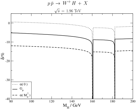
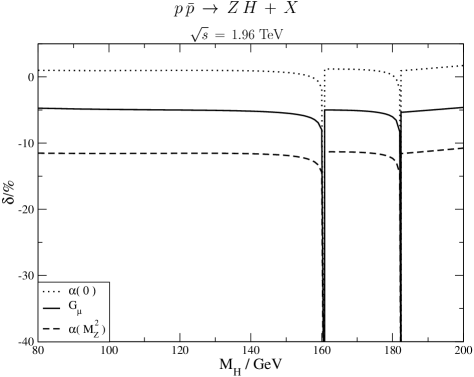
Figure 11: Relative electroweak correction $\delta$ as a function of the Higgs-boson mass for the total cross section $p\bar{p}\to W^{+}H+X$ ($\sqrt{s}=1.96\;\mathrm{TeV}$). Results are presented for the $\alpha(0)$-, $\alpha(M_{\mathrm{Z}}^{2})$-, and $G_{\mu}$-schemes.

Figure 12: Relative electroweak correction $\delta$ as a function of the Higgs-boson mass for the total cross section $p\bar{p}\to ZH+X$ ($\sqrt{s}=1.96\;\mathrm{TeV}$).

In this subsection we present the impact of the electroweak ${\cal O}(\alpha)$ corrections on the cross section predictions for the processes $p\bar{p}/pp\to W^{+}H+X$ and $p\bar{p}/pp\to ZH+X$ at the Tevatron and the LHC. Figures 12 and 12 show the relative size of the ${\cal O}(\alpha)$ corrections as a function of the Higgs-boson mass for $p\bar{p}\to W^{+}H+X$ and $p\bar{p}\to ZH+X$ at the Tevatron. Results are presented for the three different input-parameter schemes. The corrections in the $G_{\mu}$- and $\alpha(M_{\mathrm{Z}}^{2})$-schemes are significant and reduce the cross section by 5–9% and by 10–15%, respectively. The corrections in the $\alpha(0)$-scheme differ from those in the $G_{\mu}$-scheme by $2\Delta r\approx 6\%$ and from those in the $\alpha(M_{\mathrm{Z}}^{2})$-scheme by $2\Delta\alpha(M_{\mathrm{Z}}^{2})\approx 12\%$. The fact that the relative corrections in the $\alpha(0)$-scheme are rather small results from accidental cancellations between the running of the electromagnetic coupling, which leads to a contribution of about $2\Delta\alpha(M_{\mathrm{Z}}^{2})\approx+12\%$, and other (negative) corrections of non-universal origin. Thus, corrections beyond ${\cal O}(\alpha)$ in the $\alpha(0)$-scheme cannot be expected to be suppressed as well. In all schemes, the size of the corrections does not depend strongly on the Higgs-boson mass. The unphysical singularities at the thresholds $M_{H}=2M_{W}$ and $2M_{Z}$ can be removed by taking into account the finite widths of the unstable particles, see e.g. Refs. [32]. Representative results for the leading-order cross section and the electroweak ${\cal O}(\alpha)$ corrections are collected in Tables 2 and 2.

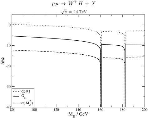
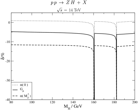
Figure 13: Relative electroweak correction $\delta$ as a function of the Higgs-boson mass for the total cross section $pp\to W^{+}H+X$ ($\sqrt{s}=14\;\mathrm{TeV}$).

Figure 14: Relative electroweak correction $\delta$ as a function of the Higgs-boson mass for the total cross section $pp\to ZH+X$ ($\sqrt{s}=14\;\mathrm{TeV}$).

Figures 14 and 14 and Tables 4 and 4 show the corresponding results for $pp\to W^{+}H+X$ and $pp\to ZH+X$ at the LHC. The corrections are similar in size to those at the Tevatron and reduce the cross section by 5–10% in the $G_{\mu}$-scheme and by 12–17% in the $\alpha(M_{\mathrm{Z}}^{2})$-scheme. We note that the electroweak corrections to $pp\to W^{-}H+X$ at the LHC differ from those to $pp\to W^{+}H+X$ by less than about $2\%$.

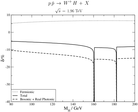
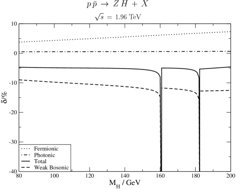
Figure 15: Different contributions to the relative electroweak correction $\delta$ in the $G_{\mu}$-scheme as a function of the Higgs-boson mass for the total cross section $p\bar{p}\to W^{+}H+X$ ($\sqrt{s}=1.96\;\mathrm{TeV}$).

Figure 16: Different contributions to the relative electroweak correction $\delta$ in the $G_{\mu}$-scheme as a function of the Higgs-boson mass for the total cross section $p\bar{p}\to ZH+X$ ($\sqrt{s}=1.96\;\mathrm{TeV}$).

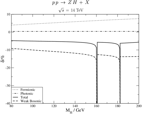
Figure 17: Different contributions to the relative electroweak correction $\delta$ in the $G_{\mu}$-scheme as a function of the Higgs-boson mass for the total cross section $pp\to W^{+}H+X$ ($\sqrt{s}=14\;\mathrm{TeV}$).

Figure 18: Different contributions to the relative electroweak correction $\delta$ in the $G_{\mu}$-scheme as a function of the Higgs-boson mass for the total cross section $pp\to ZH+X$ ($\sqrt{s}=14\;\mathrm{TeV}$).

In order to unravel the origin of the electroweak corrections we display the contributions of individual gauge-invariant building blocks. Figure 16 separates the fermionic corrections (comprising all diagrams with closed fermion loops) from the remaining bosonic contributions to $p\bar{p}\to W^{+}H+X$ at the Tevatron in the $G_{\mu}$-scheme. We observe that the bosonic corrections are dominant and that bosonic and fermionic contributions partly compensate each other. A similar result is found for the $p\bar{p}\to ZH+X$ cross section, where we display the gauge-invariant contributions from (photonic) QED corrections, fermionic corrections, and weak bosonic corrections in Fig. 16. Note that large logarithmic corrections from initial-state photon radiation have been absorbed into the quark distribution functions. The remainder of the QED corrections turns out to be strongly suppressed with respect to the fermionic and weak bosonic corrections. A similar pattern is observed for the $pp\to W^{+}H+X$ and $pp\to ZH+X$ cross sections at the LHC, see Figs. 18 and 18.

At first sight, the large size of the non-universal corrections, i.e. corrections that are not due to the running of $\alpha(k^{2})$, photon radiation, or other universal effects, might be surprising. However, a similar pattern has already been observed in the electroweak corrections to the processes ${\mathrm{e^{+}}}{\mathrm{e^{-}}}\to ZH$ [13] and ${\mathrm{e^{+}}}{\mathrm{e^{-}}}\to Z^{*}H\to\nu\bar{\nu}H$ [33, 16]. Also there large non-universal fermionic and bosonic corrections of opposite sign occur. It was also observed that the corrections cannot be approximated by simple formulae resulting from appropriate asymptotic limits. For instance, taking the large top-mass limit ($m_{\mathrm{t}}\to\infty$) in the fermionic corrections to $WH$ production in the $G_{\mu}$-scheme (see Sect. 2.2.2), the leading term in the relative correction is given by $\delta^{\mathrm{top}}_{q\bar{q}^{\prime}\to WH}\Big{|}_{G_{\mu}}\approx-1.6\%$, which even differs in sign from the full result (see Fig. 16). The reason for this failure is that the relevant scale in the $WWH$ vertex, from which the leading $m_{\mathrm{t}}^{2}$ term in the limit $m_{\mathrm{t}}\to\infty$ results, is set by the variable $\hat{s}$ which is not much smaller than but rather of the same order as $m_{\mathrm{t}}^{2}$. For the $ZH$ channel, we get $\delta^{\mathrm{top}}_{u\bar{u}\to ZH}\Big{|}_{G_{\mu}}\approx\delta^{\mathrm{top}}_{d\bar{d}\to ZH}\Big{|}_{G_{\mu}}\approx-1\%$, again reflecting the failure of the heavy-top limit as a suitable approximation. Concerning the weak bosonic corrections, large negative contributions are expected in the high-energy limit owing to the occurrence of Sudakov logarithms of the form $-\alpha/\pi\log^{2}(\hat{s}/M_{\mathrm{W}}^{2})$. However, the relevant partonic CM energies $\sqrt{\hat{s}}$ are not yet large enough for the Sudakov logarithms to provide a good approximation for the full corrections.

4.3 The cross section at NLO

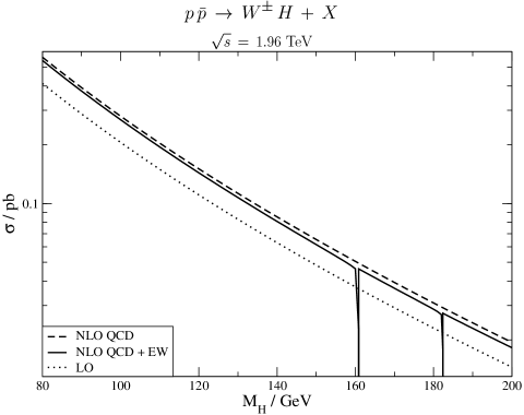
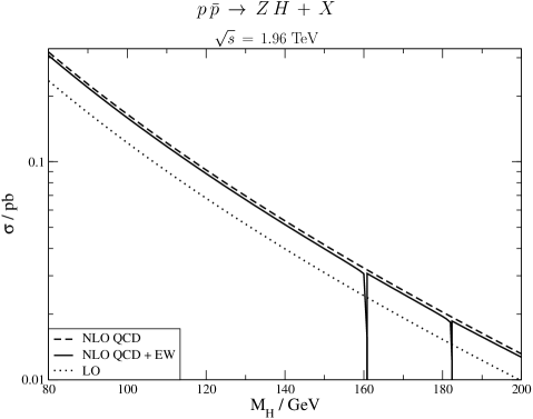
Figure 19: Total cross section for $p\bar{p}\to W^{\pm}H+X$ (sum of $W^{+}H$ and $W^{-}H$) at the Tevatron ($\sqrt{s}=1.96\;\mathrm{TeV}$) in LO, NLO QCD, and including NLO QCD and electroweak corrections in the $G_{\mu}$-scheme. The renormalization and factorization scales have been set to the invariant mass of the Higgs–vector-boson pair, $\mu=\sqrt{s_{VH}}$. CTEQ6L1 and CTEQ6M [31] parton distribution functions have been adopted at LO and ${\cal O}(\alpha_{\rm s})$, respectively.

Figure 20: Total cross section for $p\bar{p}\to ZH+X$ at the Tevatron ($\sqrt{s}=1.96\;\mathrm{TeV}$) in LO, NLO QCD, and including NLO QCD and electroweak corrections in the $G_{\mu}$-scheme.

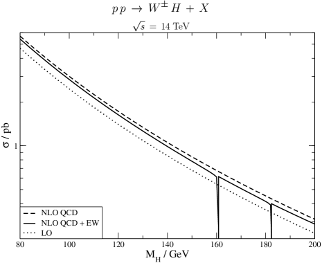
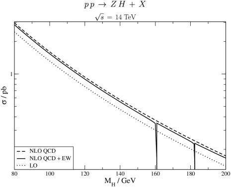
Figure 21: Total cross section for $pp\to W^{\pm}H+X$ at the LHC ($\sqrt{s}=14\;\mathrm{TeV}$) in LO, NLO QCD, and including NLO QCD and electroweak corrections in the $G_{\mu}$-scheme.

Figure 22: Total cross section for $pp\to ZH+X$ at the LHC ($\sqrt{s}=14\;\mathrm{TeV}$) in LO, NLO QCD, and including NLO QCD and electroweak corrections in the $G_{\mu}$-scheme.

In this subsection we present the cross section prediction for associated $WH$ and $ZH$ production at the Tevatron and at the LHC, including the NLO order electroweak and QCD corrections, and we quantify the residual theoretical uncertainty due to scale variation and the parton distribution functions. The total cross sections for the processes $p\bar{p}/pp\to W^{\pm}H+X$ (sum of $W^{+}H$ and $W^{-}H$) and $p\bar{p}/pp\to ZH+X$ at the Tevatron and the LHC are displayed in Figs. 20–22. Representative results are listed in Tables 6–8. For the central renormalization and factorization scale $\mu=\mu_{0}=\sqrt{s_{VH}}$ the NLO QCD corrections increase the LO cross section by typically 20–25%. As discussed in detail in Sect. 4.2, the NLO electroweak corrections are sizeable and decrease the cross section by 5–10% in the $G_{\mu}$-scheme. The size of the ${\cal O}(\alpha_{\rm s})$ and ${\cal O}(\alpha)$ corrections does not depend strongly on the Higgs-boson mass.

The NLO prediction is very stable under variation of the QCD renormalization and factorization scales. We have varied both scales independently in the range $\mu_{0}/5<\mu<5\mu_{0}$. For both the Tevatron and the LHC, the cross section increases monotonically with decreasing renormalization scale. At the Tevatron, the maximal (minimal) cross section is obtained choosing both the renormalization and factorization scales small (large). At the LHC, in contrast, the maximal (minimal) cross section corresponds to choosing a large (small) factorization scale. From the numbers listed in Tables 6–8 one can conclude that the theoretical uncertainty introduced by varying the QCD scales in the range $\mu_{0}/5<\mu<5\mu_{0}$ is less than approximately $10\%$. We have verified that the QED factorization-scale dependence of the ${\cal O}(\alpha)$-corrected cross section is below $1\%$ and thus negligible compared to the other theoretical uncertainties. The QED scale dependence should be reduced further when using QED-improved parton densities.

We have also studied the uncertainty in the cross-section prediction due to the error in the parametrization of the parton densities. To this end we have compared the NLO cross section evaluated using the default CTEQ6 [31] parametrization with the cross section evaluated using the MRST2001 [35] parametrization. The results are collected in Tables 10–12. Both the CTEQ and MRST parametrizations include parton-distribution-error packages which provide a quantitative estimate of the corresponding uncertainties in the cross sections. Using the parton-distribution-error packages and comparing the CTEQ and MRST2001 parametrizations, we find that the uncertainty in predicting the processes $p\bar{p}/pp\to W^{\pm}H+X$ and $p\bar{p}/pp\to ZH+X$ at the Tevatron and the LHC due to the parametrization of the parton densities is less than approximately $5\%$.

5 Conclusions

We have calculated the electroweak ${\cal O}(\alpha)$ corrections to Higgs-boson production in association with $W$ or $Z$ bosons at hadron colliders. These corrections decrease the theoretical prediction by up to 5–10%, depending in detail on the Higgs-boson mass and the input-parameter scheme. We have updated the cross section prediction for associated $WH$ and $ZH$ production at the Tevatron and at the LHC, including the next-to-leading order electroweak and QCD corrections. Finally, the remaining theoretical uncertainty has been studied by varying the renormalization and factorization scales and by taking into account the uncertainties in the parton distribution functions. We find that the scale dependence is reduced to about $10\%$ at next-to-leading order, while the uncertainty due to the parton densities is less than about $5\%$.

$M_{H}/\mathrm{GeV}$ $\sigma_{0}|_{\alpha(0)}/\mathrm{pb}$ $\delta|_{\alpha(0)}/\%$ $\sigma_{0}|_{\alpha(M_{Z}^{2})}/\mathrm{pb}$ $\delta|_{\alpha(M_{Z}^{2})}/\%$ $\sigma_{0}|_{G_{\mu}}/\mathrm{pb}$ $\delta|_{G_{\mu}}/\%$ 80.00 0.1926(1) 0.57(1) 0.2175(1) $-11.99(1)$ 0.2058(1) $-5.17(1)$ 100.00 0.09614(1) 0.25(1) 0.1086(1) $-12.29(1)$ 0.1028(1) $-5.61(1)$ 120.00 0.05176(1) $-0.17(1)$ 0.05846(1) $-12.75(1)$ 0.05532(1) $-6.19(1)$ 140.00 0.02945(1) $-0.89(1)$ 0.03327(1) $-13.53(1)$ 0.03149(1) $-7.05(1)$ 170.00 0.01367(1) $-2.55(1)$ 0.01544(1) $-15.30(1)$ 0.01461(1) $-8.90(1)$ 190.00 0.008517(1) $-1.97(1)$ 0.009624(1) $-14.66(1)$ 0.009106(1) $-8.38(1)$

Table 1: Total lowest-order hadronic cross section $\sigma_{0}(p\bar{p}\;\to\;W^{+}\,H+X)$ and corresponding relative electroweak correction $\delta$ ($\sqrt{s}=1.96\;\mathrm{TeV}$). Results are presented for the $\alpha(0)$-, $\alpha(M_{\mathrm{Z}}^{2})$-, and $G_{\mu}$-schemes. The integration error is given in brackets.

$M_{H}/\mathrm{GeV}$ $\sigma_{0}|_{\alpha(0)}/\mathrm{pb}$ $\delta|_{\alpha(0)}/\%$ $\sigma_{0}|_{\alpha(M_{Z}^{2})}/\mathrm{pb}$ $\delta|_{\alpha(M_{Z}^{2})}/\%$ $\sigma_{0}|_{G_{\mu}}/\mathrm{pb}$ $\delta|_{G_{\mu}}/\%$ 80.00 0.2199(1) 0.99(1) 0.2484(1) $-11.52(1)$ 0.2350(1) $-4.73(1)$ 100.00 0.1142(1) 0.95(1) 0.1290(1) $-11.57(1)$ 0.1221(1) $-4.91(1)$ 120.00 0.06358(1) 0.97(1) 0.07182(1) $-11.55(1)$ 0.06796(1) $-5.01(1)$ 140.00 0.03727(1) 0.91(1) 0.04211(1) $-11.61(1)$ 0.03984(1) $-5.18(1)$ 170.00 0.01799(1) 1.12(1) 0.02032(1) $-11.38(1)$ 0.01922(1) $-5.10(1)$ 190.00 0.01148(1) 1.26(1) 0.01297(1) $-11.24(1)$ 0.01227(1) $-5.04(1)$

Table 2: Total lowest-order hadronic cross section $\sigma_{0}(p\bar{p}\;\to\;Z\,H+X)$ and corresponding relative electroweak correction $\delta$ ($\sqrt{s}=1.96\;\mathrm{TeV}$).

$M_{H}/\mathrm{GeV}$ $\sigma_{0}|_{\alpha(0)}/\mathrm{pb}$ $\delta|_{\alpha(0)}/\%$ $\sigma_{0}|_{\alpha(M_{Z}^{2})}/\mathrm{pb}$ $\delta|_{\alpha(M_{Z}^{2})}/\%$ $\sigma_{0}|_{G_{\mu}}/\mathrm{pb}$ $\delta|_{G_{\mu}}/\%$ 80.00 2.660(1) 0.31(1) 3.005(1) $-12.22(2)$ 2.844(1) $-5.43(1)$ 100.00 1.410(1) $-0.11(1)$ 1.594(1) $-12.67(2)$ 1.508(1) $-5.99(1)$ 120.00 0.8114(2) $-0.65(1)$ 0.9166(2) $-13.24(2)$ 0.8673(2) $-6.67(1)$ 140.00 0.4967(1) $-1.49(1)$ 0.5610(1) $-14.16(2)$ 0.5309(1) $-7.68(1)$ 170.00 0.2605(1) $-3.33(1)$ 0.2942(1) $-16.12(2)$ 0.2784(1) $-9.72(2)$ 190.00 0.1776(1) $-2.92(1)$ 0.2007(1) $-15.67(2)$ 0.1899(1) $-9.36(1)$

Table 3: Total lowest-order hadronic cross section $\sigma_{0}(pp\;\to\;W^{+}\,H+X)$ and corresponding relative electroweak correction $\delta$ ($\sqrt{s}=14\;\mathrm{TeV}$).

$M_{H}/\mathrm{GeV}$ $\sigma_{0}|_{\alpha(0)}/\mathrm{pb}$ $\delta|_{\alpha(0)}/\%$ $\sigma_{0}|_{\alpha(M_{Z}^{2})}/\mathrm{pb}$ $\delta|_{\alpha(M_{Z}^{2})}/\%$ $\sigma_{0}|_{G_{\mu}}/\mathrm{pb}$ $\delta|_{G_{\mu}}/\%$ 80.00 2.299(1) 0.95(1) 2.595(1) $-11.56(1)$ 2.457(1) $-4.77(1)$ 100.00 1.232(1) 0.83(1) 1.392(1) $-11.68(1)$ 1.317(1) $-5.03(1)$ 120.00 0.7134(1) 0.76(1) 0.8058(1) $-11.77(1)$ 0.7630(1) $-5.22(1)$ 140.00 0.4381(1) 0.54(1) 0.4950(1) $-12.01(1)$ 0.4684(1) $-5.56(1)$ 170.00 0.2297(1) 0.37(1) 0.2595(1) $-12.18(1)$ 0.2456(1) $-5.88(1)$ 190.00 0.1563(1) 0.32(1) 0.1765(1) $-12.23(1)$ 0.1670(1) $-6.01(1)$

Table 4: Total lowest-order hadronic cross section $\sigma_{0}(pp\;\to\;Z\,H+X)$ and corresponding relative electroweak correction $\delta$ ($\sqrt{s}=14\;\mathrm{TeV}$).

$M_{H}/\mathrm{GeV}$ $\sigma_{0}|_{G_{\mu}}/\mathrm{pb}$ $\sigma^{\rm QCD}_{\rm NLO}/\mathrm{pb}$ $\sigma^{\rm QCD+EW}_{\rm NLO}/\mathrm{pb}$ $\sigma^{\rm QCD+EW}_{\rm NLO}/\mathrm{pb}\rule[-8.53581pt]{0.0pt}{25.60747pt}$ $\mu_{R}=5\mu_{0}$ $\mu_{R}=\mu_{0}/5$ $\mu_{F}=5\mu_{0}$ $\mu_{F}=\mu_{0}/5$ 80.00 0.4117(1) 0.5616(2) 0.5404(2) 0.5033(1) 0.5838(1) 100.00 0.2056(1) 0.2801(1) 0.2685(1) 0.2482(1) 0.2911(1) 120.00 0.1106(1) 0.1504(1) 0.1436(1) 0.1318(1) 0.1562(1) 140.00 0.06297(1) 0.08536(1) 0.08092(1) 0.07377(1) 0.08833(1) 170.00 0.02921(1) 0.03940(1) 0.03679(1) 0.03318(1) 0.04037(1) 190.00 0.01821(1) 0.02446(1) 0.02294(1) 0.02056(1) 0.02525(1)

Table 5: Total cross section for $p\bar{p}\to W^{\pm}H+X$ (sum of $W^{+}H$ and $W^{-}H$) at the Tevatron ($\sqrt{s}=1.96\;\mathrm{TeV}$) in LO, NLO QCD, and including NLO QCD and electroweak corrections in the $G_{\mu}$-scheme. The renormalization scale ($\mu_{R}$) and the factorization scale ($\mu_{F}$) have been set to the invariant mass of the Higgs–vector-boson pair, $\mu=\mu_{0}=\sqrt{s_{VH}}$. CTEQ6L1 and CTEQ6M [31] parton distribution functions have been adopted at LO and ${\cal O}(\alpha_{\rm s})$, respectively. The last two columns show the minimal and maximal cross section prediction obtained from varying the QCD renormalization and factorization scales independently in the range $\mu_{0}/5<\mu<5\mu_{0}$.

$M_{H}/\mathrm{GeV}$ $\sigma_{0}|_{G_{\mu}}/\mathrm{pb}$ $\sigma^{\rm QCD}_{\rm NLO}/\mathrm{pb}$ $\sigma^{\rm QCD+EW}_{\rm NLO}/\mathrm{pb}$ $\sigma^{\rm QCD+EW}_{\rm NLO}/\mathrm{pb}\rule[-8.53581pt]{0.0pt}{25.60747pt}$ $\mu_{R}=5\mu_{0}$ $\mu_{R}=\mu_{0}/5$ $\mu_{F}=5\mu_{0}$ $\mu_{F}=\mu_{0}/5$ 80.00 0.2350(1) 0.3181(1) 0.3070(1) 0.2858(1) 0.3317(1) 100.00 0.1221(1) 0.1649(1) 0.1589(1) 0.1470(1) 0.1722(1) 120.00 0.06796(1) 0.09160(1) 0.08820(1) 0.08111(2) 0.09575(1) 140.00 0.03984(1) 0.05354(1) 0.05148(1) 0.04706(2) 0.05604(1) 170.00 0.01922(1) 0.02570(1) 0.02472(1) 0.02242(1) 0.02701(1) 190.00 0.01227(1) 0.01635(1) 0.01573(1) 0.01418(1) 0.01722(1)

Table 6: Total cross section for $p\bar{p}\to ZH+X$ at the Tevatron ($\sqrt{s}=1.96\;\mathrm{TeV}$) in LO, NLO QCD, and including NLO QCD and electroweak corrections in the $G_{\mu}$-scheme.

$M_{H}/\mathrm{GeV}$ $\sigma_{0}|_{G_{\mu}}/\mathrm{pb}$ $\sigma^{\rm QCD}_{\rm NLO}/\mathrm{pb}$ $\sigma^{\rm QCD+EW}_{\rm NLO}/\mathrm{pb}$ $\sigma^{\rm QCD+EW}_{\rm NLO}/\mathrm{pb}\rule[-8.53581pt]{0.0pt}{25.60747pt}$ $\mu_{R}=5\mu_{0}$ $\mu_{R}=\mu_{0}/5$ $\mu_{F}=\mu_{0}/5$ $\mu_{F}=5\mu_{0}$ 80.00 4.679(2) 5.676(2) 5.423(2) 4.875(2) 5.749(5) 100.00 2.462(1) 3.005(1) 2.859(1) 2.606(2) 3.033(2) 120.00 1.405(1) 1.726(1) 1.633(1) 1.505(1) 1.731(1) 140.00 0.8537(2) 1.054(1) 0.9892(3) 0.9204(3) 1.050(1) 170.00 0.4434(1) 0.5504(1) 0.5078(1) 0.4782(1) 0.5388(3) 190.00 0.3003(1) 0.3745(1) 0.3466(1) 0.3285(1) 0.3675(2)

Table 7: Total cross section for $pp\to W^{\pm}H+X$ at the LHC ($\sqrt{s}=14\;\mathrm{TeV}$) in LO, NLO QCD, and including NLO QCD and electroweak corrections in the $G_{\mu}$-scheme.

$M_{H}/\mathrm{GeV}$ $\sigma_{0}|_{G_{\mu}}/\mathrm{pb}$ $\sigma^{\rm QCD}_{\rm NLO}/\mathrm{pb}$ $\sigma^{\rm QCD+EW}_{\rm NLO}/\mathrm{pb}$ $\sigma^{\rm QCD+EW}_{\rm NLO}/\mathrm{pb}\rule[-8.53581pt]{0.0pt}{25.60747pt}$ $\mu_{R}=5\mu_{0}$ $\mu_{R}=\mu_{0}/5$ $\mu_{F}=\mu_{0}/5$ $\mu_{F}=5\mu_{0}$ 80.00 2.457(1) 2.974(1) 2.857(1) 2.578(2) 3.018(3) 100.00 1.317(1) 1.605(1) 1.539(1) 1.407(1) 1.629(1) 120.00 0.7630(1) 0.9346(3) 0.8947(3) 0.8271(2) 0.9462(6) 140.00 0.4684(2) 0.5768(2) 0.5508(2) 0.5138(1) 0.5830(3) 170.00 0.2456(1) 0.3045(1) 0.2900(1) 0.2736(1) 0.3068(2) 190.00 0.1670(1) 0.2078(1) 0.1978(1) 0.1879(1) 0.2094(1)

Table 8: Total cross section for $pp\to ZH+X$ at the LHC ($\sqrt{s}=14\;\mathrm{TeV}$) in LO, NLO QCD, and including NLO QCD and electroweak corrections in the $G_{\mu}$-scheme.

$M_{H}/\mathrm{GeV}$ CTEQ6M [31] MRST2001 [35] 80.00 0.5404(2) $\pm$ 0.021 0.5448(2) $\pm$ 0.0097 100.00 0.2685(1) $\pm$ 0.011 0.2698(1) $\pm$ 0.0052 120.00 0.1436(1) $\pm$ 0.0060 0.1437(1) $\pm$ 0.0030 140.00 0.08092(1) $\pm$ 0.0035 0.08065(1) $\pm$ 0.0018 170.00 0.03679(1) $\pm$ 0.0017 0.03644(1) $\pm$ 0.00091 190.00 0.02294(1) $\pm$ 0.0011 0.02262(1) $\pm$ 0.00060

Table 9: Parton distribution function (PDF) uncertainties: Total cross section for $p\bar{p}\to W^{\pm}H+X$ at the Tevatron ($\sqrt{s}=1.96\;\mathrm{TeV}$) including NLO QCD and electroweak corrections in the $G_{\mu}$-scheme for different sets of parton distribution functions. The results include an estimate of the uncertainty due to the parametrization of the parton densities as obtained with the CTEQ6 [31] and MRST2001 [35] eigenvector sets (columns 2 and 3, respectively). The renormalization and the factorization scales have been set to the invariant mass of the Higgs–vector-boson pair, $\mu=\mu_{0}=\sqrt{s_{VH}}$.

$M_{H}/\mathrm{GeV}$ CTEQ6M [31] MRST2001 [35] 80.00 0.3070(1) $\pm$ 0.012 0.3090(1) $\pm$ 0.0039 100.00 0.1589(1) $\pm$ 0.0064 0.1596(1) $\pm$ 0.0020 120.00 0.08820(1) $\pm$ 0.0036 0.08840(1) $\pm$ 0.0011 140.00 0.05148(1) $\pm$ 0.0021 0.05151(1) $\pm$ 0.00066 170.00 0.02472(1) $\pm$ 0.0010 0.02469(1) $\pm$ 0.00033 190.00 0.01573(1) $\pm$ 0.00068 0.01568(1) $\pm$ 0.00021

Table 10: PDF uncertainties: Total cross section for $p\bar{p}\to ZH+X$ at the Tevatron ($\sqrt{s}=1.96\;\mathrm{TeV}$) including NLO QCD and electroweak corrections in the $G_{\mu}$-scheme for different sets of parton distribution functions.

$M_{H}/\mathrm{GeV}$ CTEQ6M [31] MRST2001 [35] 80.00 5.423(2) $\pm$ 0.18 5.509(2) $\pm$ 0.071 100.00 2.859(1) $\pm$ 0.096 2.910(1) $\pm$ 0.035 120.00 1.633(1) $\pm$ 0.055 1.664(1) $\pm$ 0.021 140.00 0.9892(3) $\pm$ 0.034 1.010(1) $\pm$ 0.012 170.00 0.5078(1) $\pm$ 0.018 0.5193(1) $\pm$ 0.0063 190.00 0.3466(1) $\pm$ 0.012 0.3547(2) $\pm$ 0.0043

Table 11: PDF uncertainties: Total cross section for $pp\to W^{\pm}H+X$ at the LHC ($\sqrt{s}=14\;\mathrm{TeV}$) including NLO QCD and electroweak corrections in the $G_{\mu}$-scheme for different sets of parton distribution functions.

$M_{H}/\mathrm{GeV}$ CTEQ6M [31] MRST2001 [35] 80.00 2.857(1) $\pm$ 0.095 2.936(1) $\pm$ 0.036 100.00 1.539(1) $\pm$ 0.051 1.583(1) $\pm$ 0.019 120.00 0.8947(3) $\pm$ 0.030 0.9217(3) $\pm$ 0.011 140.00 0.5508(2) $\pm$ 0.019 0.5681(2) $\pm$ 0.0067 170.00 0.2900(1) $\pm$ 0.010 0.2994(1) $\pm$ 0.0036 190.00 0.1978(1) $\pm$ 0.0069 0.2045(1) $\pm$ 0.0025

Table 12: PDF uncertainties: Total cross section for $pp\to ZH+X$ at the LHC ($\sqrt{s}=14\;\mathrm{TeV}$) including NLO QCD and electroweak corrections in the $G_{\mu}$-scheme for different sets of parton distribution functions.

References

-
[1]
P. W. Higgs,
Phys. Lett. 12 (1964) 132;
Phys. Rev. Lett. 13 (1964) 508
and Phys. Rev. 145 (1966) 1156;
F. Englert and R. Brout, Phys. Rev. Lett. 13 (1964) 321;
G. S. Guralnik, C. R. Hagen and T. W. Kibble, Phys. Rev. Lett. 13 (1964) 585;
T. W. Kibble, Phys. Rev. 155 (1967) 1554. - [2] The LEP Working Group for Higgs Boson Searches, LHWG Note/2002-01.
- [3] The LEP Electroweak Working Group and the SLD Heavy Flavor and Electroweak Groups, D. Abbaneo et al., LEPEWWG/2003-01.
- [4] Report of the Tevatron Higgs working group, M. Carena, J. S. Conway, H. E. Haber, J. D. Hobbs et al. [hep-ph/0010338].
-
[5]
ATLAS Collaboration, Technical Design Report, Vols. 1 and 2, CERN–LHCC–99–14
and CERN–LHCC–99–15;
CMS Collaboration, Technical Proposal, CERN–LHCC–94–38. -
[6]
S. L. Glashow, D. V. Nanopoulos and A. Yildiz,
Phys. Rev. D 18 (1978) 1724;
Z. Kunszt, Z. Trócsány and W. J. Stirling, Phys. Lett. B 271 (1991) 247. -
[7]
T. Han and S. Willenbrock,
Phys. Lett. B 273, 167 (1991);
J. Ohnemus and W. J. Stirling, Phys. Rev. D 47 (1993) 2722;
H. Baer, B. Bailey and J. F. Owens, Phys. Rev. D 47 (1993) 2730;
S. Mrenna and C. P. Yuan, Phys. Lett. B 416 (1998) 200 [hep-ph/9703224];
M. Spira, Fortsch. Phys. 46 (1998) 203 [hep-ph/9705337]. -
[8]
D. A. Dicus and S. S. Willenbrock,
Phys. Rev. D 34 (1986) 148;
D. A. Dicus and C. Kao, Phys. Rev. D 38 (1988) 1008 [Erratum-ibid. D 42 (1990) 2412];
V. D. Barger, E. W. Glover, K. Hikasa, W. Y. Keung, M. G. Olsson, C. J. Suchyta and X. R. Tata, Phys. Rev. Lett. 57 (1986) 1672;
B. A. Kniehl, Phys. Rev. D 42 (1990) 2253. -
[9]
R. Hamberg, W. L. van Neerven and T. Matsuura,
Nucl. Phys. B 359 (1991) 343;
W. L. van Neerven and E. B. Zijlstra, Nucl. Phys. B 382 (1992) 11. - [10] U. Baur, S. Keller and D. Wackeroth, Phys. Rev. D 59 (1999) 013002 [hep-ph/9807417].
- [11] S. Dittmaier and M. Krämer, Phys. Rev. D 65 (2002) 073007 [hep-ph/0109062].
-
[12]
U. Baur, S. Keller and W. K. Sakumoto,
Phys. Rev. D 57 (1998) 199
[hep-ph/9707301];
U. Baur, O. Brein, W. Hollik, C. Schappacher and D. Wackeroth, Phys. Rev. D 65 (2002) 033007 [hep-ph/0108274]. -
[13]
J. Fleischer and F. Jegerlehner,
Nucl. Phys. B 216 (1983) 469;
B. A. Kniehl, Z. Phys. C 55 (1992) 605;
A. Denner, J. Küblbeck, R. Mertig and M. Böhm, Z. Phys. C 56 (1992) 261. - [14] F. Jegerlehner, DESY 01-029, LC-TH-2001-035 [hep-ph/0105283].
- [15] A. Denner, Fortsch. Phys. 41 (1993) 307.
- [16] A. Denner, S. Dittmaier, M. Roth and M. M. Weber, Nucl. Phys. B 660 (2003) 289 [hep-ph/0302198].
-
[17]
J. Küblbeck, M. Böhm and A. Denner,
Comput. Phys. Commun. 60 (1990) 165;
H. Eck and J. Küblbeck, Guide to FeynArts 1.0, University of Würzburg, 1992. - [18] T. Hahn, Comput. Phys. Commun. 140 (2001) 418 [hep-ph/0012260].
- [19] G. Passarino and M. Veltman, Nucl. Phys. B 160 (1979) 151.
-
[20]
G. ’t Hooft and M. Veltman,
Nucl. Phys. B 153 (1979) 365;
W. Beenakker and A. Denner, Nucl. Phys. B 338 (1990) 349;
A. Denner, U. Nierste and R. Scharf, Nucl. Phys. B 367 (1991) 637. -
[21]
R. Mertig, M. Böhm and A. Denner,
Comput. Phys. Commun. 64 (1991) 345;
R. Mertig, Guide to FeynCalc 1.0, University of Würzburg, 1992. - [22] T. Hahn, Nucl. Phys. Proc. Suppl. 89 (2000) 231 [hep-ph/0005029].
-
[23]
A. Sirlin,
Phys. Rev. D 22 (1980) 971;
W. J. Marciano and A. Sirlin, Phys. Rev. D 22 (1980) 2695 [Erratum-ibid. D 31 (1980) 213] and Nucl. Phys. B 189 (1981) 442. - [24] B. A. Kniehl and M. Steinhauser, Nucl. Phys. B 454 (1995) 485 [hep-ph/9508241].
-
[25]
T. Stelzer and W. F. Long,
Comput. Phys. Commun. 81 (1994) 357
[hep-ph/9401258];
F. Maltoni and T. Stelzer, JHEP 0302 (2003) 027 [hep-ph/0208156]. - [26] H. Murayama, I. Watanabe and K. Hagiwara, KEK-91-11.
- [27] S. Dittmaier, Nucl. Phys. B 565 (2000) 69 [hep-ph/9904440].
- [28] S. Catani and M. H. Seymour, Phys. Lett. B 378 (1996) 287 [hep-ph/9602277] and Nucl. Phys. B 485 (1997) 291 [Erratum-ibid. B 510 (1997) 291] [hep-ph/9605323].
-
[29]
J. Kripfganz and H. Perlt,
Z. Phys. C 41 (1988) 319;
H. Spiesberger, Phys. Rev. D 52 (1995) 4936 [hep-ph/9412286]. - [30] K. Hagiwara et al. [Particle Data Group Collaboration], Phys. Rev. D 66 (2002) 010001.
- [31] J. Pumplin, D. R. Stump, J. Huston, H. L. Lai, P. Nadolsky and W. K. Tung, JHEP 0207 (2002) 012 [hep-ph/0201195].
-
[32]
T. Bhattacharya and S. Willenbrock,
Phys. Rev. D 47 (1993) 4022;
B. A. Kniehl, C. P. Palisoc and A. Sirlin, Phys. Rev. D 66 (2002) 057902 [hep-ph/0205304]. -
[33]
G. Belanger et al.,
hep-ph/0211268;
Phys. Lett. B 559 (2003) 252
[hep-ph/0212261];
A. Denner, S. Dittmaier, M. Roth and M. M. Weber, Phys. Lett. B 560 (2003) 196 [hep-ph/0301189]. -
[34]
C. S. Li and S. H. Zhu,
Phys. Lett. B 444 (1998) 224
[hep-ph/9801390];
Q. H. Cao, C. S. Li and S. H. Zhu, Commun. Theor. Phys. 33 (2000) 275 [hep-ph/9810458]. - [35] A. D. Martin, R. G. Roberts, W. J. Stirling and R. S. Thorne, Eur. Phys. J. C 28 (2003) 455 [arXiv:hep-ph/0211080].
- [36] A. D. Martin, R. G. Roberts, W. J. Stirling and R. S. Thorne, Eur. Phys. J. C 23 (2002) 73 [arXiv:hep-ph/0110215].