Next-to-leading order QCD calculations with parton showers I: collinear singularities

Abstract

Programs that calculate observables in quantum chromodynamics at next-to-leading order typically suffer from the problem that, when considered as event generators, the events generated consist of partons rather than hadrons and just a few partons at that. Thus the events generated are completely unrealistic. These programs would be much more useful if the few partons were turned into parton showers, in the style of standard Monte Carlo event generators. Then the parton showers could be given to one of the Monte Carlo event generators to produce hadron showers. We show how to generate parton showers related to the final state collinear singularities of the next-to-leading order perturbative calculation for the example of $e^{+}+e^{-}\to 3\ {\rm jets}$. The soft singularities are left for a separate publication.

I Introduction

Perturbation theory is a powerful tool for deriving the consequences of the standard model and its extensions in order to compare to experimental results. When strongly interacting particles are involved, perturbation theory becomes relevant when the experiment involves a short distance process, with a momentum scale $Q$ that is large compared to 1 GeV. Then one can expand the theoretical quantities for the short distance part of the reaction in powers of $\alpha_{s}(Q)$, which is small for large $Q$. Of course, the particles continue to interact at long distances, but for suitable types of experiments the long distance effects in the final state can be neglected while the long distance effects in the initial state can be factored into parton distribution functions that describe the distributions of partons in incoming hadrons. This works if the measurement of properties of the final state is infrared safe: the measurement is only weakly affected by long distance interactions in the final state. Examples include the inclusive production of very heavy particles and the production of (suitably defined) jets of light particles.

The simplest sort of calculation for this purpose consists of calculating the hard process cross section at the lowest order in $\alpha_{s}$, call it $\alpha_{s}^{B}$, at which it occurs. For example, for two-jet production in hadron-hadron collisions, $B=2$ while for three-jet production in electron-positron annihilation $B=1$. This kind of lowest order (LO) calculation is simple, but leaves out numerically significant contributions. Corrections from higher order graphs are often found to be 50% of the lowest order result. For this reason, one often performs a next-to-leading order (NLO) calculation, including terms proportional to $\alpha_{s}^{B}$ and $\alpha_{s}^{B+1}$. Then the estimated error from yet higher order terms (which are usually unknown) is typically smaller, say 10%.

There is another kind of calculational technique available, that of the Monte Carlo event generator Pythia ; Herwig ; Ariadne . In this technique, a computer program generates “events,” a list of particles ($\pi$, $\rho$, $p$, …) and their momenta $p_{1},p_{2},p_{3},\dots$ that constitute a final state that could arise from the given collision. Call the $n$th final state $f_{\!n}$. The program is constructed in such a way that the probability of generating a final state $f$ is approximately proportional to the physical probability of getting this same final state in the standard model or in whatever theory is to be tested. That is, the predicted value for an observable described by a measurement function ${\cal S}(f)$ is

$$\langle{\cal S}\rangle={1\over N}\sum_{n=1}^{N}{\cal S}(f_{\!n}).$$ (1)

Alternatively, the program may generate weights $w_{n}$ for the events, so that

$$\langle{\cal S}\rangle={1\over N}\sum_{n=1}^{N}w_{n}\,{\cal S}(f_{\!n}).$$ (2)

The Monte Carlo event generators have proven to be of enormous value. Among their benefits is the following. Since they generate complete final states, one can use detector simulations to analyze the effects on the measurement of any departure of the detector from an ideal detector. Essentially, this amounts to replacing an idealized measurement function ${\cal S}(f)$ by something that is much closer to what an actual detector does.

There are, of course, some weaknesses in Monte Carlo event generators, considered as tools to provide predictions of the standard model and its extensions. One is that the theory encoded in them is more than the standard model. They also contain models and approximations for long and medium distance physics. Fortunately, the long and medium distance effects do not matter much in the case that the measurement function ${\cal S}(f)$ is infrared safe and involves only one large momentum scale $Q$. In this case, the place where the medium and long distance approximations are important is in assessing the effects of detector imperfections, which likely result in having an effective measurement function, ${\cal S}_{\rm eff}(f)$, including the detector effects, that departs somewhat from the ideal function ${\cal S}(f)$ and thus departs from being truly infrared safe.

A more serious weakness of current Monte Carlo event generators is that they are based on leading order perturbation theory, so that a rather substantial theoretical uncertainty should be ascribed to the result if the result is considered as deduction from the standard model (or one of its extensions) with no other hypotheses included.

Return now to the NLO calculations. They are typically computer programs that act as Monte Carlo generators of partonic events. They produce events $f$ consisting of a few partons with specified momenta. For example, for three-jet production in electron-positron annihilation, there are three or four partons in the final state. Each event comes with a weight $w_{n}$. Then the predicted value for an observable described by a measurement function ${\cal S}(f)$ is

$$\langle{\cal S}\rangle={1\over N}\sum_{n=1}^{N}w_{n}\,{\cal S}(f_{\!n}).$$ (3)

Here $S(f)$ is an idealized measurement function applied to the partonic final state. We see that the NLO programs are actually quite close in structure to the Monte Carlo event generators.

One perceived weakness of the NLO Monte Carlo generators is that the weights are negative as well as positive. This feature arises because the programs do real quantum mechanics, in which an amplitude times a complex conjugate amplitude has a real part that can be either positive or negative. Negative weights do not, however, cause a problem when inserted into Eq. (3): computers can easily multiply negative numbers.

The real weakness of most current NLO Monte Carlo generators is that they produce simulated final states that are not close to physical final states. What could be done to generate realistic final states? Following the example of the leading order event generators, which do generate realistic final states, one would use the final states in the NLO partonic generators to generate a parton shower from each outgoing parton. This gives a final state with lots of partons. Then one could use one of the highly successful algorithms of the leading order Monte Carlo event generators to turn the many partons into hadrons. There should not be a serious problem with the hadronization stage, since this is modeled as a long distance process that leaves infrared safe observables largely unchanged. The problem lies with the parton showers. Here a high energy parton splits into two daughter partons, which each split into two more partons. As this process continues, the virtualities of successive pairs of daughter partons gets smaller and smaller, representing splittings that happen at larger and larger distance scales. The late splittings leave infrared safe observables largely unchanged. However, the first splittings in a parton shower can involve large virtualities. They represent a mixture of long distance and short distance physics. Thus one must be careful that the showering does not reproduce some piece of short distance physics that was already included in the NLO calculation.

Consider an example that illustrates these ideas, jet production in $pp$ collisions with $\sqrt{s}=14\ {\rm TeV}$ at the Large Hadron Collider now under construction. One can calculate the inclusive cross section $d\sigma/dM_{JJ}$ to make two jets with a dijet mass $M_{JJ}$. We may specify that the jets are defined with the $k_{T}$ algorithm kTjets , that we integrate over the rapidities of the two jets in the range $|y_{1}|<1,|y_{2}|<1$, and that $M_{JJ}$ is in the range $0.5\ {\rm TeV}<M_{JJ}<5\ {\rm TeV}$. There are computer programs currently available to perform this calculation at NLO EKS ; giele ; nagy . There are no large logarithms in the theory in this kinematic region. Thus an NLO calculation should be reliable. If the experiment were to disagree with the theory beyond the experimental errors and the estimated errors from uncalculated NNLO contributions and from parton distributions, that would be a significant indication that some sort of physics not included in the standard model is at work.

Although the theoretical picture just outlined seems bright, the available programs do not produce realistic final states. To illustrate this, imagine computing a cross section that is sensitive to the final state. For example, one might use a standard NLO program to calculate the cross section $d\sigma/dM_{JJ}dM_{1}$, where $M_{1}$ is the mass of the jet with the larger rapidity. Our result would not be sensible in the region $M_{1}\ll M_{JJ}$. It would have a nonintegrable singularity at $M_{1}=0$ together with a term proportional to $\delta(M_{1})$ with an infinite negative coefficient. The integral over $M_{1}$ of this highly singular function would give back $d\sigma/dM_{JJ}$, but the differential distribution would be highly nonphysical. In contrast, the standard Monte Carlo event generators can generate sensible results simultaneously for both $d\sigma/dM_{JJ}$ and $d\sigma/dM_{JJ}\,dM_{1}$. The only drawback is that the result for $d\sigma/dM_{JJ}$ will be correct only to leading order in an expansion in powers of $\alpha_{s}(M_{JJ})$. The problem addressed in this paper (using, however, an example from electron-positron annihilation) is how to modify such an NLO calculation so as to take advantage of the parton shower technology built into Monte Carlo event generators. We wish to get quantities like $d\sigma/dM_{JJ}\,dM_{1}$ approximately right while not losing the NLO accuracy of $d\sigma/dM_{JJ}=\int dM_{1}\ d\sigma/dM_{JJ}\,dM_{1}$.

Some technical language is helpful here in order to make these ideas more precise. Using the familiar concept of infrared safety (defined precisely in Sec. II), one can describe the cross section $d\sigma/dM_{JJ}$ as an infrared safe two-jet cross section. Then the cross section $d\sigma/dM_{JJ}dM_{1}$ for $M_{1}>0$ is an infrared safe three-jet cross section: it is infrared safe and is nonzero only when the number of final state particles is three or more. With this language, what we wish to do is get two-jet cross sections right to NLO and at the same time get $n$-jet cross sections approximately right for $n>2$.

Recall that the shower Monte Carlo programs work by using an approximate version of the perturbative theory at an infinite number of orders in perturbation theory, approximating the behavior of the Feynman graphs near the singularities corresponding to collinear parton splitting or soft gluon emission. These singularities lead to large logarithms, two powers of $\log(M_{1}/M_{JJ})$ for each additional power of $\alpha_{s}$. The programs approximately add up a series of $\alpha_{s}^{N}$ factors times logarithmic factors. After this, there is a phase that models how partons turn into hadrons. In this paper we omit the hadronization phase and use our own code for the parton showering. Our intention is that in the future only the stages of showering that directly connect to the hard scattering would be part of a program for NLO hard scattering with showers. The parts of the shower related to “softer” parton splittings, along with hadronization, would be performed by one of the standard Monte Carlo programs. We thus concentrate in this paper on the showering–hard-scattering interface and not on the showering itself.

We can illustrate the same points for an NLO base calculation that has one more jet. An instructive example is the cross section discussed above, $d\sigma/dM_{JJ}\,dM_{1}$. Here we do not integrate over $M_{1}$ and we insist that $M_{1}/M_{JJ}$ not be small. This is technically an infrared safe three-jet cross section, as discussed earlier. In a three or four parton system that appears in the calculation of this quantity at NLO, jet 1 consists of two or three partons and has mass $M_{1}$, while jet 2 consists of one or two partons. The NLO calculation (using nagy ) should be reliable but would not have sensible final states. Thus if we let $M_{2}$ be the mass of whichever of the two measured jets has the smaller rapidity and tried to calculate $d\sigma/dM_{JJ}\,dM_{1}\,dM_{2}$, the result would not be even approximately correct for $M_{2}\ll M_{JJ}$ and $M_{2}\ll M_{1}$. One would then like to have a method that could get quantities like $d\sigma/dM_{JJ}\,dM_{1}\,dM_{2}$ approximately right while not loosing the NLO accuracy of $d\sigma/dM_{JJ}\,dM_{1}$.

This discussion can serve to illustrate another point. Note that a calculation of $d\sigma/dM_{JJ}\,dM_{1}$ will have a problem if $M_{1}/M_{JJ}\ll 1$ because the result will contain large logarithms, namely logs of $M_{1}/M_{JJ}$. The large logarithms are associated with the partons getting close to a two-jet configuration. One could then view the event as arising from a two-jet event in which one of the jets splits into two nearly collinear jets or one hard jet and one soft jet. A two-jet calculation with showers would get the effects of these large logarithms approximately right. What one would then want is a method to merge the two-jet and three-jet calculations so that 1) a two-jet infrared safe observable is correctly calculated at order $\alpha_{s}^{3}$, i.e. NLO, 2) a three-jet infrared safe observable with suitable cuts so that the contributing events are well away from the two-jet region is correctly calculated at order $\alpha_{s}^{4}$, i.e. NLO for three-jets, and 3) a three-jet infrared safe observable with cuts that allow contributions from close to the two-jet region is correctly calculated at order $\alpha_{s}^{4}$ with additional corrections proportional to $\alpha_{s}^{n+4}$ times logs, with $n\geq 1$, that approximately account for the production of three jets by showering from a two-jet event. An investigation of this merging problem would certainly be desirable, but is beyond the scope of this paper.

This paper concerns $e^{+}+e^{-}\to 3\ {\rm{jets}}$. The goal is to see how to modify a NLO calculation by adding parton showers in such a way that when the generated events are used to calculate an infrared safe observable, the observable is calculated correctly at next-to-leading order. To do this, we build on our work in KSCoulomb , which sets up the NLO calculation in the Coulomb gauge. It is convenient to use a physical gauge for this purpose because it makes the analysis simpler. In this paper we explain the aspects of this problem that relate to the divergences that appear in perturbation theory when two massless partons become collinear. This part of the method is, we think, quite simple and easy to understand. The treatment of the divergences that appear when a gluon becomes soft is a bit more technical and will be given in a separate paper softshower .

The algorithms that we propose apply to showers from final state massless partons. They are illustrated using the process $e^{+}+e^{-}\to 3\ {\rm{jets}}$ in quantum chromodynamics and are embodied in computer code that performs calculations for this process beowulfcode . We do not discuss showers from initial state massless partons. While our research program (starting with KSCoulomb ) was underway, Frixione and Webber succeeded in matching showers to a NLO calculation for a problem with massless partons in the initial state (but no observed colored partons in the final state) FrixioneWebberI . Subsequently, Frixione, Webber, and Nason have extended this method to massive colored partons in the final state FrixioneWebberII . The general approach of FrixioneWebberI ; FrixioneWebberII is quite similar to that of the present paper with respect to collinear singularities. The principle difference is that we generate the first splittings of partons from an order $\alpha_{s}^{B}$ diagram using the functions given by the partonic self-energy diagrams in the Coulomb gauge, while FrixioneWebberI ; FrixioneWebberII uses the splitting functions of the Herwig Monte Carlo event generator.

We discuss $e^{+}+e^{-}\to 3\ {\rm{jets}}$ but not $e^{+}+e^{-}\to 2\ {\rm{jets}}$. Of course, to calculate $e^{+}+e^{-}\to 2\ {\rm{jets}}$ at order $\alpha_{s}$ with parton showering added would be quite a lot simpler than the present calculation for $e^{+}+e^{-}\to 3\ {\rm{jets}}$ at order $\alpha_{s}^{2}$. However, merging the two calculations would not be trivial and is not attempted here. We simply suppose that the present calculation is to be applied with a measurement function that gives zero for events that are close to the two-jet configuration (for example, for thrust near one).

There has been other recent work on this problem otherwork . That of Collins JCC is particularly instructive. This approach seeks both to put the parton showering calculation on a more rigorous basis and at the same time to match it to the hard scattering calculation, viewing the hard scattering as one end of a cascade of virtualities. Our goal is more limited. We take it as proven by experience that parton showers work well to make reasonably realistic final states. Our only concern is to make sure that when we add parton showers we do not lose the NLO accuracy of the result.

II Next-to-leading order calculation

We begin with a program that calculates an infrared safe observable in electron-positron annihilation at next-to-leading order. The program KSCoulomb uses a physical gauge, specifically the Coulomb gauge, and performs all of the integrals, including the virtual loop integrals, numerically beowulfPRL ; beowulfPRD ; beowulfrho . It is not really necessary to perform the virtual loop integrals numerically. It is a lot easier, but if one wanted to perform these integrals by hand ahead of time and insert the analytical results into the program, the calculation could still proceed. It is also not necessary to use a physical gauge. However, the use of a physical gauge makes the method conceptually simpler. In particular, collinear singularities are isolated in very simple Feynman subdiagrams, the cut and uncut two-point functions. If one were to use the Feynman gauge, the collinear singularities would be spread over many kinds of graphs and one would need another layer of analysis to organize them into a simple form. The Coulomb gauge, in particular, is well suited for calculations of electron-positron annihilation, in which the physics is approximately rotationally invariant in the electron-positron c.m. frame. The time-like axial gauge has this same good property, but is not well suited for our algorithm for a technical reason: it introduces singularities in the complex energy plane for loop integrals, which would make the evaluation of the energy integrals in our algorithm more complicated.

In order to present a method for adding showers to the NLO program, we need to review a little about how the NLO calculation works. We present the barest outline. Details may be found in beowulfPRL ; beowulfPRD ; beowulfrho ; KSCoulomb . In the NLO program, the observable is expressed in the form

$${\cal I} = \sum_{n}{1\over n!}\,\int d\vec{p}_{1}\cdots d\vec{p}_{n}\ \delta\left(\sum\vec{p}_{i}\right)\,{h\!\left(\sqrt{s}\right)\over\sigma_{0}\left(\sqrt{s}\,\right)}\,$$ (4)

$$\times F_{\!n}\!\left(\vec{p}_{1},\dots,\vec{p}_{n},\sqrt{s},\alpha_{s}\!\left(\sqrt{S}\right)\right){\cal S}_{n}\!\left(\vec{p}_{1}\sqrt{S/s},\dots,\vec{p}_{n}\sqrt{S/s}\right).$$

Here there is a sum over the number $n$ of final state partons. For a next-to-leading order calculation of a three-jet observable, $n$ runs from 3 to 4. The c.m. energy is $\sqrt{S}$. There are integrations over dimensionless momenta $\vec{p}_{j}$ for the final state partons. The true, dimensionful momenta are $\vec{P}_{j}=\vec{p}_{j}\sqrt{S/s}$ where $\sqrt{s}=\sum|\vec{p}_{j}|$. There is a delta function for momentum conservation. In place of the delta function for energy conservation, there is a function $h(\sqrt{s})$ that satisfies $\int d\sqrt{s}\ h(\sqrt{s})=1$. There is a conventional normalizing factor ${1/\sigma_{0}\left(\sqrt{s}\,\right)}$, where $\sigma_{0}$ is the Born cross section for $e^{+}+e^{-}\to{\rm hadrons}$.

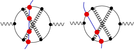
Figure 1: Two cuts of one of the Feynman diagrams that contribute to $e^{+}e^{-}\to{\rm hadrons}$.

The functions $F_{\!n}$ contain the perturbative matrix elements, calculated from the Feynman diagrams for the process. For instance, two such diagrams are depicted in Fig. 1. The first has four partons in the final state and contributes to $F_{\!4}$, while the second has three partons in the final state and contributes to $F_{\!3}$. In the case of diagrams with a virtual loop, as in the second diagram in Fig. 1, the function $F_{\!n}$ contains an integral over a dimensionless loop momentum $\vec{l}$. It is an essential part of the numerical method used here that the integration over the loop momentum is performed numerically, at the same time as the integrations over the final state momenta are performed.

At next-to-leading order, the functions $F_{\!n}$ contain either one or two powers of $\alpha_{s}$. We take the renormalization scale to be $\mu=c_{\mu}\sqrt{S}$, where $c_{\mu}$ is a dimensionless parameter. In our numerical example at the end of this paper, we take $c_{\mu}=1/6$.

The last ingredients in Eq. (4) are the measurement functions ${\cal S}_{n}$, which are functions of the dimensionful final state momenta $\vec{p}_{j}\sqrt{S/s}$. These functions are depicted in Fig. 1 by dots where parton lines cross the cut that represents the final state. The functions ${\cal S}_{n}$ represent a three-jet observable in the sense that ${\cal S}_{2}=0$. They are invariant under interchanges of their arguments and are infrared safe in the sense that

$${\cal S}_{n+1}\!\left(\vec{P}_{1},\dots,\lambda\vec{P}_{n},(1-\lambda)\vec{P}_{n}\right)={\cal S}_{n}\!\left(\vec{P}_{1},\dots,\vec{P}_{n}\right)$$ (5)

for $0\leq\lambda<1$, so that the measurement is unchanged if a parton splits into two partons moving in the same direction.

III One loop self-energy diagrams

In order to formulate parton showering properly, we need to understand how one parton splits into two at the one loop level in the Coulomb gauge. In this section, we analyze the perturbative calculation of a cut quark propagator that occurs as part of a larger graph. The analysis for gluons is essentially the same.

To set the notation, consider first the contribution at order $\alpha_{s}^{0}$:

$${\cal I}[{\rm Born}]=\int\!{d\vec{q}\over 2|\vec{q}\,|}\ {\rm Tr}\left\{\hbox to0.0pt{/\hss}q\,R_{0}\right\},$$ (6)

where $\vec{q}$ is the three-momentum carried by the propagator, $q^{\mu}=(|\vec{q}\,|,\vec{q}\,)$, and $R_{0}$ denotes the factors associated with the rest of the graph and with the final state measurement function. In particular, $R_{0}$ has two Dirac indices that match the Dirac indices on the $\hbox to0.0pt{/\hss}q$ and there is a trace over these indices.

Next, consider the contribution from a cut self-energy insertion on the quark propagator in question. The quark splits into a quark plus a gluon, giving a contribution of the form

$${\cal I}[{\rm real}]=\int\!{d\vec{q}\over 2|\vec{q}\,|}\ {\rm Tr}\left\{\int_{0}^{\infty}\!{d\bar{q}^{2}\over\bar{q}^{2}}\int_{0}^{1}\!dx\int_{-\pi}^{\pi}\!{d\phi\over 2\pi}\ {\alpha_{s}\over 2\pi}{\cal M}_{g/q}(\bar{q}^{2},x,\phi)\,R(\bar{q}^{2},x,\phi)\right\}.$$ (7)

Here there is an integration over the loop momentum that describes the splitting. We use coordinates $\left\{\bar{q}^{2},x,\phi\right\}$ for this loop momentum. We define these as follows. Let the gluon momentum be $\vec{k}_{+}$ and the quark momentum after the splitting be $\vec{k}_{-}$, with $\vec{k}_{+}+\vec{k}_{-}=\vec{q}$. We define $\bar{q}^{2}$ and $x$ by

$$\sqrt{1+\bar{q}^{2}/|\vec{q}\,|^{2}} = (|\vec{k}_{+}|+|\vec{k}_{-}|)/|\vec{q}\,|,$$

$$2x-1 = (|\vec{k}_{+}|-|\vec{k}_{-}|)/|\vec{q}\,|.$$ (8)

Then $0<\bar{q}^{2}$ and $0<x<1$. The variables $\bar{q}^{2}$ and $x$ are constant on surfaces that are, respectively, ellipsoids and hyperboloids in loop momentum space. These surfaces are orthogonal to each other where they intersect. The virtuality of the quark-gluon pair is

$$(|\vec{k}_{+}|+|\vec{k}_{-}|)^{2}-|\vec{q}\,|^{2}=\bar{q}^{2}.$$ (9)

Finally, we let $\phi$ be the azimuthal angle of $\vec{k}_{+}$ in a coordinate frame in which the $z$ axis lies along $\vec{q}$ and the $x$ axis is defined arbitrarily.

The function $[{\alpha_{s}/(2\pi)}]{\cal M}_{g/q}(\bar{q}^{2},x,\phi)$ in Eq. (7) is determined directly from the Feynman rules and is given as ${\cal M}_{q}$ in Eq. (87) of Ref. KSCoulomb . Its $\bar{q}^{2}\to 0$ limit is simple:

$${\alpha_{s}\over 2\pi}{\cal M}_{g/q}(\bar{q}^{2},x,\phi)\sim\hbox to0.0pt{/\hss}q\,{\alpha_{s}\over 2\pi}\,\tilde{P}_{g/q}(x),$$ (10)

where $\tilde{P}_{g/q}(x)$ is the one loop Altarelli-Parisi kernel for $q\to g$, namely $C_{F}[1+(1-x)^{2}]/x$. [We follow the notation of Ref. 4, in which $\tilde{P}_{a/b}(x)$ denotes the Altarelli-Parisi kernel for $b\to a$ but omitting regulation of the $x\to 1$ singularity, if there is such a singularity for that $\{a,b\}$ combination.]

The function $R$ denotes the rest of the graph and the measurement function, as before. Because it includes the measurement function, it depends on $x$ and $\phi$ as well as on $\bar{q}^{2}$. Because the measurement function is infrared safe, the $\bar{q}^{2}\to 0$ limit of $R$ is simple:

$$R(\bar{q}^{2},x,\phi)\to R_{0}\hskip 28.45274pt{\rm as}\hskip 28.45274pt\bar{q}^{2}\to 0,$$ (11)

where $R_{0}$ is the function appearing in the Born cross section, Eq. (6).

Next, consider the contribution from virtual self-energy insertions on the quark propagator in question. The quark splits into a quark plus a gluon that recombine, leaving a single quark line in the final state. The net contribution from the two virtual loop graphs is

$${\cal I}[{\rm virtual}]=\int\!{d\vec{q}\over 2|\vec{q}\,|}\ {\rm Tr}\left\{-\int_{0}^{\infty}{d\bar{q}^{2}\over\bar{q}^{2}}\int_{0}^{1}\!dx\int_{-\pi}^{\pi}\!{d\phi\over 2\pi}\ {\alpha_{s}\over 2\pi}\,{\cal P}_{\!g/q}(\bar{q}^{2},x)\,\hbox to0.0pt{/\hss}q\,R_{0}\right\}.$$ (12)

Here, again, $q^{\mu}=(|\vec{q}\,|,\vec{q}\,)$ is the on-shell incoming momentum. The function ${\cal P}_{\!g/q}$ is given in the Appendix. It equals the function ${\cal P}_{\!q}$ calculated in Ref. KSCoulomb except for modifications to the terms that reflect renormalization. The most crucial feature of ${\cal P}_{\!g/q}$ is its $\bar{q}^{2}\to 0$ limit:

$${\cal P}_{\!g/q}(\bar{q}^{2},x)\to\tilde{P}_{g/q}(x)\hskip 28.45274pt{\rm as}\hskip 28.45274pt\bar{q}^{2}\to 0.$$ (13)

If we combine the three perturbative contributions, we have

$${\cal I}[{\rm Born}]+{\cal I}[{\rm real}]+{\cal I}[{\rm virtual}] = \int\!{d\vec{q}\over 2|\vec{q}\,|}\ {\rm Tr}\biggl{\{}\hbox to0.0pt{/\hss}q\,R_{0}+\int_{0}^{\infty}{d\bar{q}^{2}\over\bar{q}^{2}}\int_{0}^{1}\!dx\int_{-\pi}^{\pi}\!{d\phi\over 2\pi}\$$ (14)

$$\left[{\alpha_{s}\over 2\pi}{\cal M}_{g/q}(\bar{q}^{2},x,\phi)R(\bar{q}^{2},x,\phi)-{\alpha_{s}\over 2\pi}\,{\cal P}_{\!g/q}(\bar{q}^{2},x)\,\hbox to0.0pt{/\hss}q\,R_{0}\right]\biggr{\}}.\ \ \ \$$

These three terms are represented in Fig. 2. The real and virtual contributions are separately infrared divergent. However the integrands are added before the integration is performed numerically. Then the divergence cancels because of Eqs. (10), (13), and (11). (It is also important for the cancellation that the two terms match when $\bar{q}^{2}\to 0$ and $x\to 0$ at the same time, with $\bar{q}^{2}/x$ fixed.)

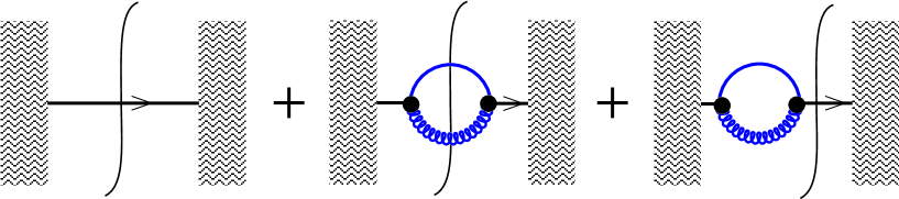
Figure 2: Graphical representation of the three terms in Eq. (14). The third diagram is intended to represent the entire virtual contribution.

IV One level shower for a single parton

So far, we see how a next-to-leading order numerical calculation works, but there is no parton shower. If we wanted to have the first splitting in a parton shower, we could follow the spirit of the parton shower Monte Carlo programs Pythia ; Herwig ; Ariadne and replace Eq. (14) by

$${\cal I}[{\rm shower}] = \int\!{d\vec{q}\over 2|\vec{q}\,|}\ {\rm Tr}\Biggl{\{}\int_{0}^{\infty}{d\bar{q}^{2}\over\bar{q}^{2}}\int_{0}^{1}\!dx\int_{-\pi}^{\pi}\!{d\phi\over 2\pi}\ {\alpha_{s}\over 2\pi}{\cal M}_{g/q}(\bar{q}^{2},x,\phi)R(\bar{q}^{2},x,\phi)$$ (15)

$$\times\exp\left(-\int_{\bar{q}^{2}}^{\infty}{d\bar{l}^{2}\over\bar{l}^{2}}\int_{0}^{1}\!dz\ {\alpha_{s}\over 2\pi}\,{\cal P}_{\!g/q}(\bar{l}^{2},z)\right)\Biggr{\}}.$$

The quantity ${\cal I}[{\rm shower}]$ is represented graphically in Fig. 3.

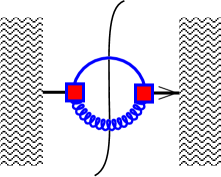
Figure 3: Graphical representation of ${\cal I}[{\rm shower}]$ in Eq. 15. The pair of square vertices represents the matrix element ${\cal M}$ and the Sudakov exponential.

In Eq. (15), we keep the construction simple by maintaining $\alpha_{s}$ evaluated at a fixed scale $\mu$. We choose not to take the $\bar{q}^{2}\to 0$ limit in any part of the function $R(\bar{q}^{2},x,\phi)$ that describes the rest of the graph. The parton splits with the exact matrix element ${\cal M}_{g/q}$, whereas a typical Monte Carlo program would use the small $\bar{q}^{2}$ limit of ${\cal M}_{g/q}$. As is standard, the exponential factor is interpreted as the probability for the parton not to split at virtuality greater than $\bar{q}^{2}$. In place of ${\cal P}_{\!g/q}$ in the exponent, one might use the Altarelli-Parisi kernel supplemented by some theta functions that keep $x$ away from 0 and 1, but we use the exact function ${\cal P}_{\!g/q}$ that occurs in the virtual corrections.

We see here that parton shower calculations as exemplified in Eq. (15) are very different from fixed order calculations as exemplified in Eq. (14). In the fixed order calculation, the virtual graph acts as a subtraction to the real splitting contribution. In the shower calculation, the virtual graph becomes a multiplicative modification to the splitting matrix element.

The perturbative representation in Eq. (14) is the same as the shower representation in Eq. (15) up to corrections of order $\alpha_{s}^{2}$:

$${\cal I}[{\rm Born}]+{\cal I}[{\rm real}]+{\cal I}[{\rm virtual}]={\cal I}[{\rm shower}]\times\left(1+{\cal O}(\alpha_{s}^{2})\right).$$ (16)

The general idea incorporated in this subtraction to multiplication theorem is a standard part of the strategy behind shower Monte Carlo programs, but we have not found the theorem stated in just this way, so we prove it here. First, we write ${\cal I}[{\rm shower}]$ as

$${\cal I}[{\rm shower}]={\cal I}_{1}[{\rm shower}]+{\cal I}_{2}[{\rm shower}]$$ (17)

with

$${\cal I}_{1}[{\rm shower}] = \int\!{d\vec{q}\over 2|\vec{q}\,|}\ {\rm Tr}\Biggl{\{}\int_{0}^{\infty}{d\bar{q}^{2}\over\bar{q}^{2}}\int_{0}^{1}\!dx\int_{-\pi}^{\pi}\!{d\phi\over 2\pi}\ \exp\left(-\int_{\bar{q}^{2}}^{\infty}{d\bar{l}^{2}\over\bar{l}^{2}}\int_{0}^{1}\!dz\ {\alpha_{s}\over 2\pi}\,{\cal P}_{\!g/q}(\bar{l}^{2},z)\right)$$ (18)

$$\times\biggl{[}{\alpha_{s}\over 2\pi}{\cal M}_{g/q}(\bar{q}^{2},x,\phi)\,R(\bar{q}^{2},x,\phi)-{\alpha_{s}\over 2\pi}\,{\cal P}_{\!g/q}(\bar{q}^{2},x)\,\hbox to0.0pt{/\hss}q\,R_{0}\biggr{]}\Biggr{\}}$$

and

$${\cal I}_{2}[{\rm shower}] = \int\!{d\vec{q}\over 2|\vec{q}\,|}\ {\rm Tr}\Biggl{\{}\hbox to0.0pt{/\hss}q\,R_{0}\int_{0}^{\infty}\!d\bar{q}^{2}\$$ (19)

$$\hskip 28.45274pt\times{1\over\bar{q}^{2}}\int_{0}^{1}\!dx\ {\alpha_{s}\over 2\pi}\,{\cal P}_{\!g/q}(\bar{q}^{2},x)\ \exp\left(-\int_{\bar{q}^{2}}^{\infty}{d\bar{l}^{2}\over\bar{l}^{2}}\int_{0}^{1}\!dz\ {\alpha_{s}\over 2\pi}\,{\cal P}_{\!g/q}(\bar{l}^{2},z)\right)\Biggr{\}}.\ \ \$$

Let us find the lowest order (up to and including order $\alpha_{s}\times R$) terms in the expansions of these integrals. The integral ${\cal I}_{1}[{\rm shower}]$ is simple. We take the order $\alpha_{s}^{0}$ term in the exponential to obtain

$${\cal I}_{1}[{\rm shower}] = \int\!{d\vec{q}\over 2|\vec{q}\,|}\ {\rm Tr}\Biggl{\{}\int_{0}^{\infty}{d\bar{q}^{2}\over\bar{q}^{2}}\int_{0}^{1}\!dx\int_{-\pi}^{\pi}\!{d\phi\over 2\pi}\$$ (20)

$$\times\biggl{[}{\alpha_{s}\over 2\pi}{\cal M}_{g/q}(\bar{q}^{2},x,\phi)\,R(\bar{q}^{2},x,\phi)-{\alpha_{s}\over 2\pi}\,{\cal P}_{\!g/q}(\bar{q}^{2},x)\,\hbox to0.0pt{/\hss}q\,R_{0}\biggr{]}\Biggr{\}}+{\cal O}(\alpha_{s}^{2}\times R).\ \ \$$

The integral ${\cal I}_{2}[{\rm shower}]$ is more subtle. We cannot simply expand under the integral since the integrals of each term would be divergent at small $\bar{q}^{2}$. Instead, we note that we have the integral over $\bar{q}^{2}$ of a total derivative, so that the integral is just the difference of the integrand between the integration end points:

$${\cal I}_{2}[{\rm shower}] = \int\!{d\vec{q}\over 2|\vec{q}\,|}\ {\rm Tr}\left\{\hbox to0.0pt{/\hss}q\,R_{0}\right\}[F(\infty)-F(0)],$$ (21)

where

$$F(\bar{q}^{2})=\exp\left(-\int_{\bar{q}^{2}}^{\infty}{d\bar{l}^{2}\over\bar{l}^{2}}\int_{0}^{1}\!dz\ {\alpha_{s}\over 2\pi}\,{\cal P}_{\!g/q}(\bar{l}^{\,2},z)\right).$$ (22)

Now the function ${\cal P}_{\!g/q}(\bar{l}^{\,2},z)$, which is given in the Appendix, has the important property that it is proportional to $1/\bar{l}^{\,2}$ for $\bar{l}^{\,2}\to\infty$. This insures that the integral in the exponent is convergent for $\bar{l}^{\,2}\to\infty$, so that $F(\bar{q}^{2})\to\exp(-0)=1$ as $\bar{q}^{2}\to\infty$. On the other hand, ${\cal P}_{\!g/q}(\bar{l}^{\,2},z)$ approaches ${P}_{\!g/q}(z)$ as $\bar{l}^{\,2}\to 0$. This makes the $\bar{l}^{\,2}$-integral diverge as $\bar{q}^{2}\to 0$. In fact, one gets two powers of $\log(\bar{q}^{2})$ for $\bar{q}^{2}\to 0$, one directly from the $\bar{l}^{\,2}$-integral and one from a divergence at $z\to 0$ in the $z$-integral that develops as ${\cal P}_{\!g/q}(\bar{l}^{2},z)$ gets closer and closer to ${P}_{\!g/q}(z)$. The net effect is that the exponent behaves like a positive constant times $\log^{2}(\bar{q}^{2})$ for $\bar{q}^{2}\to 0$. Thus $F(\bar{q}^{2})\to\exp(-\infty)=0$ as $\bar{q}^{2}\to 0$. The result for ${\cal I}_{2}[{\rm shower}]$ is then

$${\cal I}_{2}[{\rm shower}] = \int\!{d\vec{q}\over 2|\vec{q}\,|}\ {\rm Tr}\left\{\hbox to0.0pt{/\hss}q\,R_{0}\right\}.$$ (23)

Adding the results (20) and (23), we have the result in Eq. (14) plus ${\cal O}(\alpha_{s}^{2}\times R)$. This proves the theorem.

There is an analogous result for the gluon propagator. The trace is over Lorentz indices instead of Dirac indices. The functions ${\cal M}_{g/q}$ and ${\cal P}_{\!g/q}$ are replaced by functions ${\cal M}_{g/g}+N_{F}{\cal M}_{q/g}$ given in Ref. KSCoulomb and ${\cal P}_{\!g/g}+N_{F}{\cal P}_{\!q/g}$ given in the Appendix.

It should be evident that one can use the subtraction to multiplication theorem to add parton showers to the next-to-leading order calculation of three-jet cross sections, while keeping unchanged the first two terms in the perturbative expansion of the result. Indeed, there is more than one way to do this. Which way is best can and should be debated, but in this paper we confine ourselves to mapping out one way.

We will refer to the first splittings of the partons emerging from a Born graph as primary splittings. The basic idea for the primary splittings is this. Start with a computer program that does calculations at next-to-leading order in the Coulomb gauge. In each cut $\alpha_{s}^{1}$ graph, replace ${\cal I}[{\rm Born}]$ by ${\cal I}[{\rm shower}]$ for each cut propagator. Then take the cut order $\alpha_{s}^{2}$ graphs that have a cut self-energy subgraph plus its corresponding virtual correction. In each such graph, replace ${\cal I}[{\rm real}]+{\cal I}[{\rm virtual}]$ by $0$. (There are some complications that arise when applying this basic idea. We address the complications in subsequent sections.)

Once one understands this basic idea, one can envisage a lot of refinements. Here we will pursue one possible refinement. In ${\cal I}[{\rm shower}]$ we choose a number $\lambda_{V}$ of order 1 and divide the integration region into a low virtuality part, $0<\bar{q}^{2}<\lambda_{V}\vec{q}^{\,2}$, and a high virtuality part $\lambda_{V}\vec{q}^{\,2}<\bar{q}^{2}<\infty$. In the high virtuality term, we expand the Sudakov exponential in powers of $\alpha_{s}$ and keep only the order 0 term. This gives

$${\cal I}[{\rm shower}]=\biggl{(}{\cal I}[{\rm shower},\lambda_{V}]+{\cal I}[{\rm real},\lambda_{V}]\biggr{)}\times\left(1+{\cal O}(\alpha_{s}^{2})\right)$$ (24)

where

$${\cal I}[{\rm shower},\lambda_{V}] = \int\!{d\vec{q}\over 2|\vec{q}\,|}\ {\rm Tr}\Biggl{\{}\int_{0}^{\lambda_{V}\vec{q}^{\,2}}\!{d\bar{q}^{2}\over\bar{q}^{2}}\int_{0}^{1}\!dx\int_{-\pi}^{\pi}\!{d\phi\over 2\pi}\ {\alpha_{s}\over 2\pi}{\cal M}_{g/q}(\bar{q}^{2},x,\phi)R(\bar{q}^{2},x,\phi)$$ (25)

$$\times\exp\left(-\int_{\bar{q}^{2}}^{\infty}{d\bar{l}^{2}\over\bar{l}^{2}}\int_{0}^{1}\!dz\ {\alpha_{s}\over 2\pi}\,{\cal P}_{\!g/q}(\bar{l}^{2},z)\right)\Biggr{\}}.$$

and

$${\cal I}[{\rm real},\lambda_{V}]=\int\!{d\vec{q}\over 2|\vec{q}\,|}\ {\rm Tr}\left\{\int_{\lambda_{V}\vec{q}^{\,2}}^{\infty}\!{d\bar{q}^{2}\over\bar{q}^{2}}\int_{0}^{1}\!dx\int_{-\pi}^{\pi}\!{d\phi\over 2\pi}\ {\alpha_{s}\over 2\pi}{\cal M}_{g/q}(\bar{q}^{2},x,\phi)\,R(\bar{q}^{2},x,\phi)\right\}.$$ (26)

Then the refinement of the basic idea for the primary splittings is as follows. Start with a computer program that does calculations at next-to-leading order in the Coulomb gauge. In each cut $\alpha_{s}^{1}$ graph, replace ${\cal I}[{\rm Born}]$ by ${\cal I}[{\rm shower},\lambda_{V}]$ for each cut propagator. Then take the cut order $\alpha_{s}^{2}$ graphs that have a cut self-energy subgraph plus its corresponding virtual correction. In each such graph, replace ${\cal I}[{\rm real}]+{\cal I}[{\rm virtual}]$ by ${\cal I}[{\rm real},\lambda_{V}]$. This approach is a little more complicated than the simple approach we explained first, which amounts to choosing $\lambda_{V}=\infty$.

Why would one choose $\lambda_{V}<\infty$? Unless one has a NNLO calculation to compare to, one cannot know for sure which approach is best, since the approaches differ only at order $\alpha_{s}^{B+2}$. However, the $\lambda_{V}<\infty$ approach has the advantage that we apply the formula with Sudakov suppression of small virtuality splitting in the region of small or moderate virtuality, while we use ordinary fixed order perturbation theory in the large virtuality region where “parton shower” physics is not relevant.

Another possibility would be to modify ${\cal I}[{\rm shower}]$ by replacing ${\cal M}$ by a new function ${\cal M}^{\prime}$ and by replacing ${\cal P}$ by a new function ${\cal P}^{\prime}$. The new functions could be anything we like provided that they have the same small $\bar{q}^{2}\to 0$ limits as the original functions. They could, for example, be the splitting functions in a “standard” showering scheme based on virtuality as the evolution variable. Then, in the order $\alpha_{s}^{2}$ graphs, ${\cal M}$ would be replaced by ${\cal M}-{\cal M}^{\prime}$ and ${\cal P}$ would be replaced by ${\cal P}-{\cal P}^{\prime}$. Thus the shower functions ${\cal M}^{\prime}$ and ${\cal P}^{\prime}$ would act as collinear subtraction terms in the order $\alpha_{s}^{2}$ graphs. This is similar to what is done for initial state collinear singularities in FrixioneWebberI ; FrixioneWebberII . The treatment discussed above with a virtuality cutoff $\lambda_{V}<\infty$ is a special case of this more general possibility. We do not pursue the general ${\cal M}^{\prime}$, ${\cal P}^{\prime}$ possibility here.

V Primary splittings for a whole graph

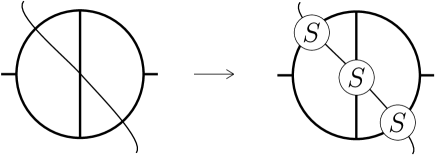
Figure 4: A cut Born graph. We depict here only the topology of the graph, leaving unspecified which lines are quarks and which are gluons. On the right, we show the graph after replacing the cut propagators by ${\cal I}[{\rm shower}]$, which is represented by a circle containing an $S$.

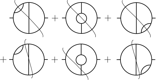
Figure 5: Six order $\alpha_{s}^{2}$ cut Feynman graphs. (For a graph with a self-energy insertion with one adjacent propagator cut, we understand the complete virtual correction.) These graphs are the order $\alpha_{s}^{2}$ term in the expansion of the graph in Fig. 4.

Let us see how this algorithm works in a particular example, taking $\lambda_{V}=\infty$ for simplicity. Begin with a cut Born (i.e. order $\alpha_{s}^{1}$) graph with the topology shown on the left in Fig. 4. The primary splitting algorithm is to replace $\cal{I}[{\rm Born}]$ by $\cal{I}[{\rm shower}]$ for each of the three parton lines crossing the cut. This is illustrated in the right hand side of Fig. 4.

When this expression is expanded in powers of $\alpha_{s}$, it gives the Born graph back along with the six order $\alpha_{s}^{2}$ graphs depicted in Fig. 5. There are further contributions that are of order $\alpha_{s}^{3}$ and higher. Since we get the graphs in Fig. 5 from the expansion of the right hand diagram in Fig. 4, we delete these contributions from the order $\alpha_{s}^{2}$ graphs.

VI Primary splittings for another graph

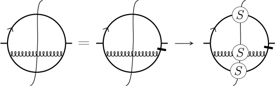
Figure 6: A cut Born graph and its replacement according to the level 1 showering algorithm.

There is one more topology for a cut Born graph that contributes to three-jet cross sections. This topology is exemplified by the graph shown as the left hand diagram in Fig. 6. Again, we keep this analysis as simple as possible by treating the case that the virtuality cut is $\lambda_{V}=\infty$.

To treat this graph, we make use of a technique that helps keep two-jet physics from affecting the three-jet cross section. Let $k_{1}$ be the momentum carried by the top propagator in Fig. 6 and let $k_{2}$ be the momentum carried by the bottom propagator before it splits into two propagators. We multiply the graph by

$$1=F_{1}(k_{1},k_{2})+F_{2}(k_{1},k_{2}),$$ (27)

where

$$F_{j}(k_{1},k_{2})={(k_{j}^{2})^{2}\over(k_{1}^{2})^{2}+(k_{2}^{2})^{2}}.$$ (28)

We separate the two terms and treat them separately, considering the factor $F_{j}$ as part of the graph. We can indicate which term is which by drawing a line through the propagator that carries momentum $k_{j}$ when we have multiplied by $F_{j}$. The line indicates that the corresponding propagator is blocked from going on-shell because of the factor $(k_{j}^{2})^{2}$. For the graph under consideration, only the $F_{2}$ term contributes, as indicated by the equality between the left and middle graphs of Fig 6.

Now we adopt as the splitting algorithm for this case the replacement of each cut propagator by ${\cal I}[{\rm shower}]$, as indicated by the right hand graph in Fig 6. It is significant that we do this only after inserting the factor $F_{2}$.

The role of the factor $F_{j}$ is easy to understand on an intuitive basis. It is possible for the graph on the left in Fig. 6 to generate a two-jet event in which the gluon is nearly parallel to the antiquark at the bottom of the graph. When each parton is allowed to split, one could get a high virtuality splitting from the quark at the top of the graph, creating a three-jet event. Of course, we want to generate three-jet events, but our calculation is based on generating three-jet events directly from the Born graphs. The function $F_{j}$ enforces the requirement that the high virtuality splitting be the one in the Born graph.

Consider now the eight order $\alpha_{s}^{2}$ cut Feynman graphs illustrated in Fig. 7, where we have inserted factors of $1=F_{1}+F_{2}$. For all except the first graph shown, only the $F_{2}$ term survives, as indicated. For the first graph, there is a corresponding graph with a factor $F_{1}$, which is not shown and would be grouped with a different set of graphs.

Now notice that when the right hand graph of Fig. 6 is expanded in powers of $\alpha_{s}$, it reproduces the Born graph with which we started plus the graphs of Fig. 7 plus corrections that are of order $\alpha_{s}^{3}$ or higher. Thus we take the splitting algorithm for this case to be that the graphs of Fig. 7 are deleted from the calculation.

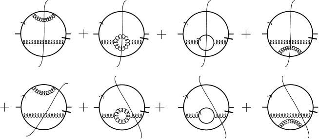
Figure 7: Eight order $\alpha_{s}^{2}$ cut Feynman graphs.

VII The next-to-leading order graphs

We have seen how to insert a one level parton splitting into the Born graphs. We have also seen that certain of the order $\alpha_{s}^{2}$ cut graphs are thereby generated, so that these graphs are to be deleted from the calculation. In the case that we have chosen $\lambda_{V}<\infty$, then the graphs that would have been deleted are retained, but with a virtuality cut $\bar{q}^{2}>\lambda_{V}\vec{q}^{\,2}$ on the appropriate cut self-energy subdiagram. Other order $\alpha_{s}^{2}$ cut graphs are not generated from the Born graphs and need to be added to the Born contributions.

VIII Secondary splittings

We have replaced each cut propagator in the Born diagrams with one step of a parton shower and have called the parton splittings generated in this way primary splittings. Now we would like to let these partons split further with secondary splittings. For each of the parton lines entering the final state, we replace $\cal{I}$ for that line by a simplified version of the splitting probability. For example, if the parton is a quark, we use

$${\cal I}[{\rm shower\mbox{-}0}] = \int\!{d\vec{q}\over 2|\vec{q}\,|}\ {\rm Tr}\Biggl{\{}\int_{0}^{\infty}{d\bar{q}^{2}\over\bar{q}^{2}}\int_{0}^{1}\!dx\int_{-\pi}^{\pi}\!{d\phi\over 2\pi}\ {\alpha_{s}\over 2\pi}\,{\cal S}_{\!g/q}(\bar{q}^{2},x)\,\hbox to0.0pt{/\hss}q\,\,R(\bar{q}^{2},x,\phi)$$ (29)

$$\times\exp\left(-\int_{\bar{q}^{2}}^{\infty}{d\bar{l}^{2}\over\bar{l}^{2}}\int_{0}^{1}\!dz\ {\alpha_{s}\over 2\pi}\,{\cal S}_{\!g/q}(\bar{l}^{2},z)\right)\Biggr{\}},$$

where the Sudakov exponent ${\cal S}_{g/q}$ is a suitable simplified version of ${\cal P}_{\!g/q}$. Here the Dirac structure, $\hbox to0.0pt{/\hss}q$, is kept exactly the same as it was in $\cal{I}[{\rm Born}]$ for this line. We thus take $q^{0}=|\vec{q}|$ in $\hbox to0.0pt{/\hss}q$. Furthermore, we take $q^{0}=|\vec{q}|$ in the rest of the graph. When this expression is expanded in powers of $\alpha_{s}$, it gives the original graph back along with some order $\alpha_{s}^{3}$ and yet higher order corrections.

In the construction so far, we have used a coupling $\alpha_{s}$ evaluated at a fixed scale, $\mu$. As a refinement, we follow standard practice by using for the showering in Eq. (29) a coupling evaluated at a running scale. We take the scale of $\alpha_{s}$ in the main line of the equation to be $[x(1-x)\bar{q}^{2}S/s_{0}]^{1/2}$ and in the exponent to be $[z(1-z)\bar{l}^{2}S/s_{0}]^{1/2}$. Recall that we use a numerical integration program that employs dimensionless momenta as integration variables. The factor $x(1-x)\bar{q}^{2}$ is the dimensionless squared transverse momentum that is associated with the splitting. A factor $S/s$ would convert to the physical momenta. We use instead $S/s_{0}$, where $\sqrt{s_{0}}=\sum|\vec{k}_{j}|$ is the sum of the absolute values of the dimensionless momenta in the perturbative diagram before splittings. Of course, when we introduce a running coupling inside an integral as in Eq. (15), we create an ambiguity about how to evaluate $\alpha_{s}(k)$ when $k\lesssim\Lambda_{\rm QCD}$. We resolve the ambiguity by freezing $\alpha_{s}(k)$, so that it ceases to grow with decreasing $k$ as soon as it reaches the value $\alpha_{s}=1$.

The function ${\cal S}_{\!g/q}(\bar{q}^{2},x)$ should be fairly simple, its integral in the Sudakov exponent should be finite, and it should approach the Altarelli-Parisi function $\tilde{P}_{g/q}(x)$ as $\bar{q}^{2}\to 0$. The reader may choose his or her favorite function. We have tried the following choice, which satisfies these criteria, for the purposes of this paper,

$${\cal S}_{\!g/q}(\bar{q}^{2},x)=\tilde{P}_{g/q}(x)\ \theta(\bar{q}^{2}<x(1-x)\kappa^{2}).$$ (30)

Here $\kappa^{2}$ serves as a cutoff parameter for the splitting. The theta function may be regarded as a simplified version of the factors $4x(1-x)/[\bar{q}^{2}/\vec{q}^{\,2}+4x(1-x)]$ that occur in the functions ${\cal P}$ that represent the virtual self-energy diagrams and appear in the Sudakov exponent of the primary splittings. (See the Appendix for the functions ${\cal P}$.) We examine what to choose for $\kappa$ below.

We can now move on to generate parton splittings within the previous parton splittings. We do this indefinitely except that, when $\bar{q}^{2}$ for a splitting is smaller than some predetermined cutoff, we regard the splitting as having gone too far. We then replace the two daughters by the mother, canceling the splitting. The mother parton remains in the final state and no further splitting of it is attempted.

Since the mother parton in the current splitting was created in a previous splitting, one can choose $\kappa^{2}$ so as to insure angular ordering between the two splittings. For a nearly collinear splitting with parameters $\{\bar{q}^{2},x,|\vec{q}|\}$ of a mother parton with momentum $\vec{q}$, the angle $\theta$ between the two daughter partons is given approximately by

$$\theta^{2}={\bar{q}^{2}\over x(1-x)\vec{q}^{\,2}}.$$ (31)

Suppose that the previous splitting had parameters $\{\bar{p}^{2},y,|\vec{q}|/y\}$, with $y$ being the momentum fraction of the daughter parton that becomes the mother parton for the second splitting. Then the angle between the two partons in the first splitting can be estimated as

$$\theta_{0}^{2}\approx\min\left[{y\,\bar{p}^{2}\over(1-y)\vec{q}^{\,2}},1\right].$$ (32)

The first expression here uses the small angle approximation, while the second provides a rough upper bound for the case that the angle is not small. Thus if we take

$$\kappa^{2}=\min\left[{y\,\bar{p}^{2}\over(1-y)},\vec{q}^{\,2},\kappa_{\rm mother}^{2}\right],$$ (33)

the probability for the second splitting is zero when the second angle is greater than the first. Here $\kappa_{\rm mother}$ is the $\kappa$ parameter that was used for generating the splitting that gave the mother parton in the current splitting.

We have not yet specified what the splitting scale $\kappa^{2}$ should be for the first secondary splitting, the splitting of one of the partons that was generated in a primary splitting. We should be a bit careful because the function $R$ used in the proof in Secs. III and IV now includes the measurement function convoluted with the functions describing the secondary splittings. In the notation of the preceding paragraph, $R(\bar{p}^{2},y,\phi)$ should approach $R_{0}$ when $\bar{p}^{2}\to 0$. This will happen if $\kappa^{2}\to 0$ (so that the secondary jets become narrow) when $\bar{p}^{2}\to 0$. For this reason, we take

$$\kappa^{2}=\min\left[{y\,\bar{p}^{2}\over(1-y)},\vec{q}^{\,2},c_{\kappa}\,\bar{p}^{2}\right],$$ (34)

where $c_{\kappa}$ is a constant, taken to be 4 in the numerical example studied in Sec. X.

IX Singularities of the next-to-leading order graphs

In the next-to-leading order calculation without showers, the order $\alpha_{s}^{2}$ cut graphs contain divergences arising from soft and collinear parton configurations. These divergences cancel between different cuts of a given graph, that is between real and virtual parton contributions.

In the Coulomb gauge, the collinear divergences arise from self-energy graphs. When we incorporate parton showers the collinear divergences disappear. If we use Eq. (16), we simply eliminate the self-energy graphs associated with final state particles, and with them we eliminate the collinear divergences. With the small modification in Eq. (24), we retain part of the real splitting self-energy graph in which the virtuality $\bar{q}^{2}$ is bigger than $\lambda_{V}\vec{q}^{\,2}$. This still eliminates the collinear divergence. As mentioned in Sec. IV, we could adopt suitably behaved alternative functions ${\cal M}^{\prime}$ and ${\cal P}^{\prime}$ to replace ${\cal M}$ and ${\cal P}$ in the splitting from a Born level graph. Then the order $\alpha_{s}^{2}$ real and virtual self-energy graphs would still be present, but ${\cal M}$ would be replaced by ${\cal M}-{\cal M}^{\prime}$ in the real graphs and ${\cal P}$ would be replaced by ${\cal P}-{\cal P}^{\prime}$ in the virtual graphs. Thus the shower functions ${\cal M}^{\prime}$ and ${\cal P}^{\prime}$ would act as collinear subtraction terms in the real and virtual order $\alpha_{s}^{2}$ graphs. In this case also, the collinear divergences are eliminated separately from the real and virtual graphs.

This leaves only the soft divergences in the order $\alpha_{s}^{2}$ graphs. The soft gluon singularities are an essential part of QCD. Their structure is quite different from that of the collinear singularities. Their treatment will be the subject of another paper softshower . Once the soft singularities are accounted for, one can let each parton from an order $\alpha_{s}^{2}$ graph create a shower. Meanwhile, the treatment given here, without showers from the order $\alpha_{s}^{2}$ graphs, yields a divergence-free calculation because the soft gluon divergences cancel between different cuts of a given graph. We will exhibit some results from this calculation in the following section.

X A numerical test

In this section, we provide a numerical test of the algorithm presented here. We have computed the thrust distribution $d\sigma/dt$ for thrust $t=0.86$, in the middle of the three-jet region. We compute the thrust distribution using the algorithm described in this paper. That is, for self-energy graphs in the limited virtuality region, we replace “${\it Born}\times[1+{\it real}-|{\it virtual}|]$” by “${\it Born}\times{\it real}\,\exp(-|{\it virtual}|)$.” Secondary showering from the Born graphs is also included. On the other hand, in this test there are no showers from the order $\alpha_{s}^{B+1}$ graphs.

The idea is to compare the thrust distribution thus calculated to the same distribution calculated with a straightforward NLO computation with no showers. According to the analysis presented above, the difference between the two calculations should be of order $\alpha_{s}^{B+2}$. We divide the difference by the NLO result, forming

$$R=\frac{\mbox{\rm(NLO-shower)}-{\rm NLO}}{{\rm NLO}}.$$ (35)

The ratio $R$ should have a perturbative expansion that begins at order $\alpha_{s}^{2}$. We can test this by plotting the ratio against $\alpha_{s}^{2}$. We expect to see a curve that approximates a straight line through zero for small $\alpha_{s}^{2}$. For comparison, we exhibit also the ratio with the $\alpha_{s}^{B+1}$ corrections omitted,

$$R_{\rm LO}=\frac{\mbox{\rm(LO-shower)}-{\rm NLO}}{{\rm NLO}}.$$ (36)

The ratio $R_{\rm LO}$ should have a perturbative expansion that begins at order $\alpha_{s}^{1}$. Thus we expect to see a curve proportional to the square root function $[{\alpha_{s}^{2}}]^{1/2}$ for small $\alpha_{s}^{2}$. (The size of the coefficient of $[{\alpha_{s}^{2}}]^{1/2}$ in $R_{\rm LO}$ does not have any great significance, since it is quite sensitive to the choice of renormalization scale.) A comparison of the two curves, $R$ and $R_{\rm LO}$, shows whether the $\alpha_{s}^{B+1}$ corrections, which are lacking in $R_{\rm LO}$, are doing their job.

The results of this test are shown in Fig. 8 for $\sqrt{S}=M_{Z}$ and for a range of $\alpha_{s}(M_{Z})$ from $(1/2)\times 0.118$ to $2\times 0.118$, where 0.118 represents something close to the physical value for $\alpha_{s}(M_{Z})$. We choose the renormalization scale to be $\mu=\sqrt{S}/6$. One should note that $2\times 0.118$ amounts to quite a large $\alpha_{s}$ in this calculation since $\alpha_{s}(M_{Z})=0.236$ gives $\alpha_{s}(\mu)=0.586$.

We see the expected shape of the $R_{\rm LO}$ curve. We also see that the $R$ curve lies closer to zero, indicating that the $\alpha_{s}^{B+1}$ corrections are acting in the right direction. The more exacting test is to examine whether the $R$ curve approaches a straight line through the origin as $\alpha_{s}^{2}\to 0$. Within the errors, it does. However, the slope of the straight line is quite small. That is presumably an accident of the choice of parameters in the program. It remains for the future to examine the effects of various parameter choices.

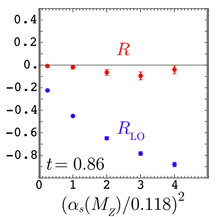
Figure 8: Comparison of the NLO calculation with showers partially added as described in this paper to a pure NLO calculation using beowulfcode . We plot the ratio $R$ defined in Eq. (35) for the thrust distribution at thrust equal 0.86. Also shown is the ratio $R_{\rm LO}$, defined in Eq. (36), in which the order $\alpha_{s}^{B+1}$ correction terms are omitted from the calculation. The c.m. energy is $\sqrt{S}=M_{Z}$ and the renormalization scale is chosen to be $\mu=\sqrt{S}/6$. These ratios are calculated for $\alpha_{s}(M_{Z})^{2}=\{0.25,1,2,3,4\}\times(0.118)^{2}$ and plotted versus $\alpha_{s}(M_{Z})^{2}/(0.118)^{2}$.

In Fig. 9, we show the same comparison, but this time for $t=0.71$. This is near the value $t=2/3$ that marks the far end of the three-jet region, with the three partons in what is sometimes called the Mercedes configuration. In this case, the $R$ curve again approaches a straight line through the origin as $\alpha_{s}^{2}\to 0$, again with quite a small slope.

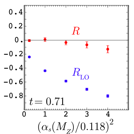
Figure 9: Comparison of the NLO calculation with showers partially added to a pure NLO calculation for $t=0.71$. The notation is as in Fig. 8.

In Fig. 10, we show the same comparison, but this time for $t=0.95$. This is near the two-jet limit at $t=1$. For $\alpha_{s}=0.118$, one would normally not use a calculation that did not include a summation of logs of $1-t$ for $t$ this close to 1, since $\log(0.05)^{2}\approx 9$. Thus we would not recommend using the code discussed in this paper for a comparison to data this near to the two-jet limit. Nevertheless, we can still test for the absence of an $\alpha_{s}^{1}$ term in $R$. Looking at the graph, we see that, within the errors, there is no evidence for a nonzero $\alpha_{s}^{1}$ term in $R$. We expect an $\alpha_{s}^{2}$ term, but the coefficient of $\alpha_{s}^{2}$ appears to be quite small. On the other hand, it appears that some of the higher order terms are quite substantial.

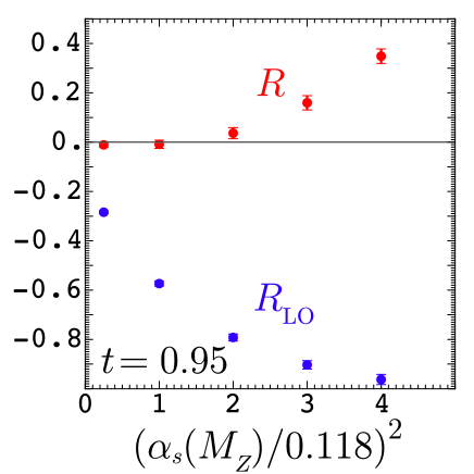
Figure 10: Comparison of the NLO calculation with showers partially added to a pure NLO calculation for $t=0.95$. The notation is as in Fig. 8.

XI Conclusions

We have presented a method for adding parton showers to a next-to-leading order calculation in QCD. Specifically, we treat the final state collinear singularities, using the example of $e^{+}+e^{-}\to 3\ {\rm jets}$. Our intention is that a program like ours would be used in conjunction with a standard Monte Carlo event generator Pythia ; Herwig ; Ariadne . The complete calculation would then act as an event generator (with positive and negative weights for the events) in which the final states consist of hadrons generated from parton showers. Recall that we defined primary parton splittings to be those of the partons emerging from an order $\alpha_{s}^{B}$ graph. There are also secondary splittings: the further splittings of the daughters from the primary splittings as well as the splittings of partons emerging from an order $\alpha_{s}^{B+1}$ graph and of their daughters. It is the primary splittings that need to be matched to the NLO calculation. The secondary splittings affect an infrared safe observable only at order $\alpha_{s}^{B+2}$. Thus the partonic events from our program after the primary splittings could be handed to a Monte Carlo event generator, which would perform the secondary splittings and the hadronization. Alternatively, our program can perform the secondary splittings, leaving hadronization for the Monte Carlo event generators. For the purpose of implementing such a scheme, it is significant that the weight functions do $\it not$ have singularities when two partons are collinear or one is soft. This is in contrast to pure NLO calculations, which depend on cancellations between different events when an infrared safe observable is calculated.

The method presented here is incomplete in that we leave for a companion publication softshower the treatment of the soft gluon singularities of QCD. The code described in this paper is available at beowulfcode . A treatment of soft gluon effects, to be described in softshower , is included in the code. Parton showers are included, but the requisite data structures and color flow information that would be necessary to provide an interface with the showering and hadronization models of standard event generator Monte Carlo programs are not yet available.

Appendix A Virtual splitting functions

In this appendix, we examine the functions ${\cal P}_{\!a/b}(\bar{q}^{2},x)$ that specify the virtual parton self-energy graphs in the Coulomb gauge.

For quark splitting, the function that we use is

$${\cal P}_{\!g/q}(\bar{q}^{2},x) = {C_{F}\over 2D_{\mu}}\,\left\{12x(1-x)-1\right\}$$ (37)

$$+{C_{F}\over 2D_{\mu}^{2}}\,{\bar{q}^{2}\over\mu_{\rm mod}^{2}}\left\{20x(1-x)-3+\log(\mu^{2}/\mu_{\rm mod}^{2})[12x(1-x)-1]\right\}$$

$$+{4C_{F}\over D_{x}}\,x(1-x)\left\{5-14x(1-x)\right\}$$

$$+{16C_{F}\over D_{x}^{2}}\,x(1-x)\left\{1-6x(1-x)+8[x(1-x)]^{2}\right\}$$

$$+{C_{F}\over 2D_{1}}\,(2x-1)$$

$$-{8C_{F}\over D_{1}D_{x}}(2x-1)x(1-x)$$

$$-{16C_{F}\over D_{1}D_{x}^{2}}(2x-1)x(1-x)\left\{1-2x(1-x)\right\},$$

where $\mu$ is the  MS  renormalization scale,

$$\mu_{\rm mod}^{2}=\min(\mu^{2},|\vec{q}\,|^{2}),$$ (38)

and

$$D_{x} = \bar{q}^{2}/|\vec{q}\,|^{2}+4x(1-x),$$

$$D_{\mu} = \bar{q}^{2}/\mu_{\rm mod}^{2}+1,$$

$$D_{1} = \bar{q}^{2}/|\vec{q}\,|^{2}+1.$$ (39)

The function ${\cal P}_{\!g/q}(\bar{q}^{2},x)$ has been modified from the function ${\cal P}_{\!q}$ given in Ref. KSCoulomb . We have replaced the two terms

$$-{C_{F}\over 2}\,{1\over e^{-3}\bar{q}^{2}/\mu^{2}+1}+C_{F}{6x(1-x)\over e^{-5/3}\bar{q}^{2}/\mu^{2}+1}$$ (40)

by the first two terms in Eq. (37). The contributions of these terms to the integral

$$\int_{\bar{q}^{2}}^{\infty}{d\bar{l}^{2}\over\bar{l}^{2}}\,{\cal P}_{\!g/q}(\bar{l}^{2},x)$$ (41)

are the same in the limit of small $\bar{q}^{2}$ up to terms that vanish as $\bar{q}^{2}\to 0$ (and are non-singular as functions of $x$). Thus the two expressions are equivalent when inserted into the perturbative formula (14).

The terms that we have modified contain the effects of  MS  renormalization. In the original form, they cut off the integral (41) at $\bar{l}^{2}$ of order $\mu^{2}$. That is a sensible way to express perturbative renormalization. However, in our present application the integral

$$\int_{\bar{q}^{2}}^{\infty}{d\bar{l}^{2}\over\bar{l}^{2}}\,\int_{0}^{1}dx\,{\cal P}_{\!g/q}(\bar{l}^{2},x)$$ (42)

appears in the Sudakov exponent for shower generation. In the case that $|\vec{q}\,|^{2}\ll\mu^{2}$, the former terms in Eq. (40) would have caused the Sudakov exponential to deviate from 1 for $\bar{q}^{2}$ much greater than $|\vec{q}\,|^{2}$. The effect of this deviation on the calculated cross section is of order $\alpha_{s}^{2}\times R_{0}$ and thus is, in principle, negligible. However this effect appears to us to be quite unphysical. The revised form of ${\cal P}_{\!g/q}$ is preferable in that it confines the contribution of the renormalization dependent terms to $\bar{q}^{2}$ of order $|\vec{q}\,|^{2}$ or smaller.

One may also note that the integral (42) is positive for all $\bar{q}^{2}$ and increases as $\bar{q}^{2}$ decreases. This was not the case with the form of ${\cal P}_{\!g/q}$ before the replacement.

For gluon splitting to a quark and antiquark, we use

$${\cal P}_{\!q/g}(\bar{q}^{2},x) = {1\over 2D_{\mu}}\,\left\{1-2x(1-x)\right\}$$

$$+{1\over 2D_{\mu}^{2}}\,{\bar{q}^{2}\over\mu_{\rm mod}^{2}}\left\{2-{\textstyle{16\over 3}}\,x(1-x)+\log(\mu^{2}/\mu_{\rm mod}^{2})[1-2x(1-x)]\right\}.$$

For gluon splitting to two gluons, we use

$${\cal P}_{\!g/g}(\bar{q}^{2},x) = {C_{A}\over D_{\mu}}\,\left\{3x(1-x)-1\right\}$$ (44)

$$+{C_{A}\over D_{\mu}^{2}}\,{\bar{q}^{2}\over\mu_{\rm mod}^{2}}\left\{7\,x(1-x)-2+\log(\mu^{2}/\mu_{\rm mod}^{2})[3x(1-x)-1]\right\}$$

$$+{12C_{A}\over D_{x}}\,x(1-x)\left\{1-2x(1-x)\right\}$$

$$+{16C_{A}\over D_{x}^{2}}\,x(1-x)\left\{1-4x(1-x)+4[x(1-x)]^{2}\right\}.$$

Here the definitions (38) and (39) apply again. For ${\cal P}_{\!q/g}$, we have replaced

$${1\over 2}\,{1\over e^{-2}\bar{q}^{2}/\mu^{2}+1}-{x(1-x)\over e^{-8/3}\bar{q}^{2}/\mu^{2}+1}$$ (45)

given in Ref. KSCoulomb by the terms in Eq. (A). For ${\cal P}_{\!g/g}$, we have replaced

$$-C_{A}\,{1\over e^{-2}\bar{q}^{2}/\mu^{2}+1}+C_{A}{x(1-x)\over e^{-5/3}\bar{q}^{2}/\mu^{2}+1}+2C_{A}{x(1-x)\over e^{-8/3}\bar{q}^{2}/\mu^{2}+1}$$ (46)

given in Ref. KSCoulomb by the first two terms in Eq. (44). The reasoning behind this modification is the same as in the case of quark splitting.

The Sudakov exponent for gluon splitting is proportional to

$$\int_{\bar{q}^{2}}^{\infty}{d\bar{l}^{2}\over\bar{l}^{2}}\,\int_{0}^{1}dx\,\left[{\cal P}_{\!g/g}(\bar{l}^{2},x)+N_{F}\,{\cal P}_{\!q/g}(\bar{l}^{2},x)\right].$$ (47)

This quantity is positive for all $\bar{q}^{2}$ and increases as $\bar{q}^{2}$ decreases provided that $N_{F}>3C_{A}/2$. Thus this form will work fine for the main cases of phenomenological interest, $C_{A}=3$ with 5 or 6 quark flavors. Further modifications would be necessary for other cases. We have not pursued this topic further because we expect that the $\cal P$ functions will be different anyway in future versions of the algorithms presented in this paper.

References

- (1) T. Sjöstrand, Comput. Phys. Commun. 39 (1986) 347; T. Sjöstrand, P. Eden, C. Friberg, L. Lönnblad, G. Miu, S. Mrenna and E. Norrbin, Comput. Phys. Commun. 135, 238 (2001) [arXiv:hep-ph/0010017].
- (2) G. Marchesini, B. R. Webber, G. Abbiendi, I. G. Knowles, M. H. Seymour and L. Stanco, Comput. Phys. Commun. 67, 465 (1992); G. Corcella et al., JHEP 0101 010 (2001) [arXiv:hep-ph/0011363].
- (3) L. Lönnblad, Comput. Phys. Commun. 71, 15 (1992).
- (4) S. D. Ellis and D. E. Soper, Phys. Rev. D 48, 3160 (1993) [arXiv:hep-ph/9305266].
- (5) S. D. Ellis, Z. Kunszt and D. E. Soper, Phys. Rev. Lett. 64, 2121 (1990).
- (6) W. T. Giele, E. W. Glover and D. A. Kosower, Nucl. Phys. B 403, 633 (1993) [arXiv:hep-ph/9302225].
- (7) Z. Nagy, Phys. Rev. Lett. 88, 122003 (2002) [arXiv:hep-ph/0110315].
- (8) M. Krämer and D. E. Soper, Phys. Rev. D 66, 054017 (2002) [arXiv:hep-ph/0204113].
- (9) D. E. Soper, arXiv:hep-ph/0306268.
- (10) D. E. Soper, beowulf Version 3.0, http://zebu.uoregon.edu/∼soper/beowulf/.
- (11) S. Frixione and B. R. Webber, JHEP 0206, 029 (2002) [arXiv:hep-ph/0204244].
- (12) S. Frixione, P. Nason and B. R. Webber, JHEP 0308, 007 (2003) [arXiv:hep-ph/0305252].
- (13) S. Mrenna, [arXiv:hep-ph/9902471]; B. Pötter, Phys. Rev. D 63, 114017 (2001) [arXiv:hep-ph/0007172]; M. Dobbs, Phys. Rev. D 64, 034016 (2001) [arXiv:hep-ph/0103174]; B. Pötter and T. Schörner, Phys. Lett. B 517, 86 (2001) [arXiv:hep-ph/0104261]; M. Dobbs, Phys. Rev. D 65, 094011 (2002) [arXiv:hep-ph/0111234]; Y. Kurihara, J. Fujimoto, T. Ishikawa, K. Kato, S. Kawabata, T. Munehisa and H. Tanaka, Nucl. Phys. B 654 (2003) 301 [arXiv:hep-ph/0212216].
- (14) J. C. Collins, JHEP 0005, 004 (2000) [arXiv:hep-ph/0001040]; J. C. Collins and F. Hautmann, JHEP 0103, 016 (2001) [arXiv:hep-ph/0009286]; Y. Chen, J. C. Collins and N. Tkachuk, JHEP 0106, 015 (2001) [arXiv:hep-ph/0105291]; J. C. Collins and X. Zu, JHEP 0206, 018 (2002) [arXiv:hep-ph/0204127].
- (15) D. E. Soper, Phys. Rev. Lett. 81, 2638 (1998) [arXiv:hep-ph/9804454].
- (16) D. E. Soper, Phys. Rev. D 62, 014009 (2000) [arXiv:hep-ph/9910292].
- (17) D. E. Soper, Phys. Rev. D 64, 034018 (2001) [arXiv:hep-ph/0103262].