hep-ph/0306219

CERN–TH/2003-138

UMN–TH–2205/03

FTPI–MINN–03/16

Updated Post-WMAP Benchmarks for Supersymmetry

M. Battaglia¹, A. De Roeck¹, J. Ellis¹, F. Gianotti¹, K. A. Olive² and L. Pape^{1 1}CERN, Geneva, Switzerland
²William I. Fine Theoretical Physics Institute,
University of Minnesota, Minneapolis, MN 55455, USA

Abstract

We update a previously-proposed set of supersymmetric benchmark scenarios, taking into account the precise constraints on the cold dark matter density obtained by combining WMAP and other cosmological data, as well as the LEP and $b\rightarrow s\gamma$ constraints. We assume that $R$ parity is conserved and work within the constrained MSSM (CMSSM) with universal soft supersymmetry-breaking scalar and gaugino masses $m_{0}$ and $m_{1/2}$. In most cases, the relic density calculated for the previous benchmarks may be brought within the WMAP range by reducing slightly $m_{0}$, but in two cases more substantial changes in $m_{0}$ and $m_{1/2}$ are made. Since the WMAP constraint reduces the effective dimensionality of the CMSSM parameter space, one may study phenomenology along ‘WMAP lines’ in the $(m_{1/2},m_{0})$ plane that have acceptable amounts of dark matter. We discuss the production, decays and detectability of sparticles along these lines, at the LHC and at linear $e^{+}e^{-}$ colliders in the sub- and multi-TeV ranges, stressing the complementarity of hadron and lepton colliders, and with particular emphasis on the neutralino sector. Finally, we preview the accuracy with which one might be able to predict the density of supersymmetric cold dark matter using collider measurements.

CERN–TH/2003-138

June 2003

1 Introduction

One of the crucial topics in the planning of analyses of data from experiments at present and future colliders is the search for supersymmetry [1]. Even the minimal supersymmetric extension of the Standard Model (MSSM), which conserves $R$ parity, has over 100 free parameters once arbitrary soft supersymmetry-breaking parameters are allowed. For this reason, much attention is focussed on the constrained MSSM (CMSSM), in which the soft supersymmetry-breaking scalar masses $m_{0}$, gaugino masses $m_{1/2}$ and trilinear parameters $A_{0}$ are each assumed to be universal at some high input scale, as in minimal supergravity and other models. These CMSSM parameters are constrained principally by the absence at LEP of new particles with masses $\mathrel{\hbox to0.0pt{\raise 2.15277pt\hbox{$<$}\hss}{\lower 2.15277pt\hbox{$\sim$}}}100$ GeV, by the agreement of $b\to s\gamma$ decay with Standard Model predictions, by the measurement of the anomalous magnetic moment of the muon, $g_{\mu}-2$, and by the range allowed for relic cold dark matter, $\Omega_{CDM}$.

Benchmark supersymmetric scenarios have a venerable history [2]. A couple of years ago, a new set of benchmark supersymmetric models was proposed in [3], consistent with all the above experimental constraints, as well as the cosmological constraint on $\Omega_{CDM}$. Subsequently, there has not been any significant change in the LEP limits on supersymmetric particles [4, 5], we are still looking forward to more sensitive searches at the Fermilab Tevatron collider, the situation of $b\to s\gamma$ decay has changed little [6], and the interpretation of the $g_{\mu}-2$ measurements remains unclear [7]. Various other benchmark scenarios have been proposed, in particular some supplementary points and lines in the CMSSM and in models with different mechanisms for supersymmetry breaking [8], benchmarks for supersymmetric Higgs physics [9], and scenarios in which the prospects for the Fermilab Tevatron collider are more favourable [10, 11].

The road(w)map for supersymmetric phenomenology has, however, been altered significantly by the recent improved determination of the allowable range of the cold dark matter density obtained by combining WMAP and other cosmological data: $0.094<\Omega_{CDM}<0.129$ at the 2-$\sigma$ level [12]. This range is consistent with earlier indications, but more precise. Within the MSSM with conserved $R$ parity, if one assumes that most of the cold dark matter consists of the lightest supersymmetric particle (LSP) and identifies this with the lightest neutralino $\chi$ [13], this WMAP constraint reduces the dimensionality of the parameter space. In the CMSSM, in particular, whereas generic regions of the $(m_{1/2},m_{0})$ planes would previously have been allowed for fixed values of $\tan\beta$ and $A_{0}$ [14], now only thin strips are permitted [15, 16] .

It is of course possible to relax the restrictions to these narrow ‘WMAP lines’ in various ways. One could consider models that violate $R$ parity, though these would also be subject to (different) astrophysical and cosmological constraints. Or one could consider alternatives to gravity-mediated supersymmetry breaking, such as anomaly- or gauge- mediated supersymmetry breaking, in which the sparticle spectra could be radically different, and/or the LSP might be a gravitino [8]. However, we do not discuss such models in this paper.

Here, we consider first the minor modifications of the previous CMSSM benchmark scenarios that bring them on to the WMAP lines. In most cases, this requires only a small change in $m_{0}$, keeping $m_{1/2}$ the same as before, as seen in Table 1. An exception is the previous benchmark H, which had been chosen at the end of one of the coannihilation ‘tails’, at the largest possible value of $m_{1/2}$. The WMAP constraint not only reduces the possible spread in $m_{0}$ for fixed $m_{1/2}$, but also reduces the allowable range of $m_{1/2}$. Therefore, our modification of benchmark H has reduced values of both $m_{1/2}$ and $m_{0}$. Another example is benchmark M, which has also been shifted significantly because the rapid-annihilation ‘funnel’ for $\tan\beta=50$ and $\mu>0$ is affected substantially by the WMAP restriction on $\Omega_{\chi}h^{2}$. More detailed discussions of these updated benchmark points are given in Section 2, where we also discuss the (generally small) extent to which the decay branching ratios differ from the previous versions of the benchmark points .

Supersymmetric spectra in post-WMAP benchmark scenarios
 
Model A’ B’ C’ D’ E’ F’ G’ H’ I’ J’ K’ L’ M’ $m_{1/2}$ 600 250 400 525 300 1000 375 935 350 750 1300 450 1840 (1500) (1150) (1900) $m_{0}$ 120 60 85 110 1530 3450 115 245 175 285 1000 300 1100 (140) (100) (90) (125) (1500) (120) (419) (180) (300) (350) (1500) $\tan{\beta}$ 5 10 10 10 10 10 20 20 35 35 35 50 50 sign($\mu$) $+$ $+$ $+$ $-$ $+$ $+$ $+$ $+$ $+$ $+$ $-$ $+$ $+$ $\alpha_{s}(m_{Z})$ 121 125 123 121 124 120 124 120 123 120 118 122 117 $m_{t}$ 175 175 175 175 171 171 175 175 175 175 175 175 175 Masses $|\mu(m_{Z})|$ 741 333 503 634 205 496 471 1026 439 843 1317 540 1764 h 115 113 116 117 114 118 117 122 116 121 118 118 124 H 884 375 578 736 1532 3491 523 1185 452 883 1176 489 1652 A 882 375 578 735 1533 3491 523 1185 451 883 1176 489 1663 H^± 886 383 584 740 1535 3492 529 1188 459 887 1180 496 1654 $\chi_{1}$ 252 98 163 220 115 430 153 402 143 320 573 187 821 $\chi_{2}$ 480 181 310 424 182 522 289 774 270 615 1105 358 1583 $\chi_{3}$ 761 346 519 655 221 523 489 1068 464 897 1413 588 1994 $\chi_{4}$ 775 365 535 662 304 885 504 1078 478 906 1421 599 1999 $\chi^{\pm}_{1}$ 480 180 309 424 174 511 290 774 270 615 1105 358 1583 $\chi^{\pm}_{2}$ 775 367 535 664 304 886 505 1079 479 907 1422 600 1999 $\tilde{g}$ 1715 715 1145 1495 869 2914 1075 2681 999 1593 3716 994 5262 $e_{L}$, $\mu_{L}$ 425 188 289 375 1544 3512 285 673 300 581 1319 430 1635 $e_{R}$, $\mu_{R}$ 261 121 180 232 1535 3471 189 433 224 405 1114 348 1300 $\nu_{e}$, $\nu_{\mu}$ 418 171 278 367 1542 3511 273 669 289 575 1317 422 1633 $\tau_{1}$ 258 112 172 225 1522 3443 162 403 155 323 971 200 920 $\tau_{2}$ 425 192 291 376 1538 3498 291 670 310 573 1268 420 1511 $\nu_{\tau}$ 418 187 277 366 1542 3497 270 661 277 555 1261 386 1502 $u_{L}$, $c_{L}$ 1202 546 834 1064 1644 3908 792 1808 755 1493 2602 965 3491 $u_{R}$, $c_{R}$ 1151 527 803 1021 1635 3867 762 1730 723 1429 2494 930 3332 $d_{L}$,$s_{L}$ 1205 552 838 1067 1646 3909 797 1810 758 1429 2603 968 3492 $d_{R}$, $s_{R}$ 1144 526 799 1016 1634 3861 759 1718 723 1495 2479 925 3309 $t_{1}$ 896 393 618 807 1050 2580 587 1380 553 1131 1935 710 2630 $t_{2}$ 1143 573 819 1013 1387 3330 777 1677 731 1372 2237 891 3054 $b_{1}$ 1101 502 765 976 1379 3323 717 1645 659 1325 2173 815 2998 $b_{2}$ 1144 528 798 1011 1622 3834 756 1695 711 1377 2242 880 3062

Table 1: Proposed post-WMAP CMSSM benchmark points and mass spectra (in GeV), as calculated using SSARD [18] and FeynHiggs [19], using the one-loop corrected effective potential computed at the electroweak scale and one-loop corrections to the chargino and neutralino masses. We recall (in parentheses) the values of $m_{1/2}$ and $m_{0}$ used in [3], in cases where they differ. As in [3], exact gauge coupling unification is enforced, resulting in the predictions for $\alpha_{s}(m_{Z})$ that are shown in units of 0.001. We use $A_{0}=0$, $m_{b}(m_{b})^{\overline{MS}}=4.25$ GeV and $m_{t}=175$ GeV for most of the points, with the exceptions of points E’ and F’, where $m_{t}=171$ GeV is used.

Then, in Section 3, we discuss systematically how the phenomenology of supersymmetric models varies with $m_{1/2}$ along the WMAP lines. We first present parametrizations of these lines appropriate for the SSARD [18] and ISASUGRA 7.67 [20] codes. We then discuss the patterns of decays of various selected sparticles. We show in particular that $\chi_{2}\to{\tilde{\tau}_{1}}\tau$ decays are generally important, though other $\chi_{2}\to{\tilde{\ell}}\ell$ decays (where $\ell\equiv e,\mu$) are also important for low $m_{1/2}$ at low $\tan\beta$. The decays $\chi_{2}\to\chi h,\chi Z$ are never very large on the WMAP lines, despite being kinematically allowed for most values of $m_{1/2}$. We then discuss the average numbers of $Z,h$ and $\tau$ particles produced per sparticle production event at the LHC. This study confirms the importance of the $\tau$ signature, with trilepton signatures also looking promising. We discuss the extent to which our various benchmark scenarios sample generic features along the WMAP lines.

Section 4 contains a discussion of sparticle detectability at various accelerators, starting with the LHC . We find that the lightest MSSM Higgs boson and all the squarks are in principle observable along the complete WMAP lines, except along parts of the rapid-annihilation ‘funnels’, whereas sleptons and other neutralinos and charginos are detectable only in the lower parts of the WMAP ranges of $m_{1/2}$. This discussion is extended in Subsection 4.2 to linear $e^{+}e^{-}$ colliders with $E_{CM}=0.5,1.0$ [21] and 3.0 or 5.0 TeV [22]. Confirming previous studies [21, 3, 8], we see that a machine with $E_{CM}=0.5$ TeV would be able to explore supersymmetry in the lower parts of the WMAP ranges of $m_{1/2}$, whereas a machine with $E_{CM}=1.0$ TeV would be able to explore supersymmetry along (almost) the entire WMAP lines. CLIC with $E_{CM}=3.0$ TeV would be able to complete the spectrum of electroweakly-interacting sparticles along the entire WMAP lines, as well as furnish detailed measurements of squarks for a large fraction of the allowed range of $m_{1/2}$ [23]. We also discuss in more detail the observability of neutralinos at the different colliders surveyed, with particular emphasis on CLIC studies.

Finally, in Section 5 we review some conclusions from our results, addressing in particular the question whether collider measurements will have the potential to determine if the LSP constitutes most of the cold dark matter in the Universe [13, 24].

2 Updated CMSSM Benchmark Points

2.1 Improved Choices of Supersymmetry-Breaking Parameters

Since the laboratory constraints on the CMSSM have not yet changed substantially since the termination of LEP [4], the only reason for updating the benchmark points we proposed previously [3] is the refined estimate of $\Omega_{CDM}h^{2}$ provided by combining the new WMAP data with those previously available [12]. Assuming that most of the cold dark matter is composed of LSPs $\chi$, previously we allowed $0.1<\Omega_{\chi}h^{2}<0.3$ (rather conservatively), whereas the WMAP analysis now allows only the range

$$0.094\;<\;\Omega_{\chi}h^{2}\;<\;0.129$$ (1)

at the 2-$\sigma$ level [12]. We see in Table 2 of [3] that all the previous benchmark points yielded relic densities $\Omega_{\chi}h^{2}$ above the range (1). Since the relic density calculations have not changed significantly since [3] in the regions of interest, the previous benchmark points must be moved.

Of the 13 benchmark points proposed previously, 5 (B, C, G, I, L) were in the ‘bulk’ regions at low $m_{1/2}$ and $m_{0}$, 4 (A, D, H, J) were along the coannihilation ‘tails’ extending to larger $m_{1/2}$ [25], 2 (K, M) were along rapid-annihilation ‘funnels’ where both $m_{1/2}$ and $m_{0}$ may grow large [26], and 2 (E, F) were in the ‘focus-point’ region at very large $m_{0}$ [27]. The WMAP constraint (1) has slimmed the ‘bulk’ region down considerably, but only minor reductions in $m_{0}$ are needed to reduce the relic density of points (B, C, G, I, L) into the range (1), as shown in Table 1. The coannihilation ‘tails’ are also much thinner than they were before, and the required reductions in $m_{0}$ for points (A, D, J) are also small. The previous point H is an exception to this rule, since it was chosen at the extreme tip of a coannihilation ‘tail’. In this case, since the upper limit in (1) is considerably reduced compared with that assumed in [3], the allowed upper limit on $m_{1/2}$ has been reduced substantially [15]. Hence we must make reductions in both $m_{1/2}$ and $m_{0}$ for point H, as also shown in Table 1. In the case of point K, the rapid-annihilation ‘funnel’ has become thinner following WMAP, and a minor adjustment in $m_{1/2}$ is sufficient, but in the case of point M, the ‘funnel’ has changed substantially, and both $m_{1/2}$ and $m_{0}$ had to be changed.

The two focus-point benchmarks (E, F) may also be adapted to the WMAP constraint (1) with small changes, as also shown in Table 1, which is based on the SSARD code. However, we take this opportunity to underline the extreme delicacy of model calculations in this region, as may be seen by comparing the results of different codes [18, 20, 28, 29] in their successive releases . The various codes do agree that there is a strip in the ‘focus-point’ region where $\Omega_{\chi}h^{2}$ is in the WMAP range (1), but the error in its location due to the experimental uncertainty in the mass of the top quark $m_{t}$ (for example) is much larger than the intrinsic width of the WMAP strip in this region. We have chosen a pole mass $m_{t}=171$ GeV for benchmarks E and F, as opposed to the choice $m_{t}=175$ GeV made for the other benchmarks, which would have required much larger values of $m_{0}$ in this focus-point region, namely $m_{0}=2550,5030$ GeV for the SSARD code, respectively. The new D0 value of $m_{t}\simeq 179$ GeV [30], if confirmed, would push the ‘focus-point’ region up to still larger $m_{0}$, whatever code is used: specifically to $m_{0}=5800,9070$ GeV for benchmarks E and F, respectively, if the SSARD code is used 

There are also significant theoretical uncertainties associated with higher-order effects [31], that are reflected in differences between different codes in their various versions. For example, for $m_{t}=175$ GeV at benchmarks E and F (with $m_{1/2}=300,1000$ GeV, respectively), the ISASUGRA 7.51, [ISASUGRA 7.67], [SUSPECT 2.10], [SUSPECT 2.11] codes require $m_{0}=1530,3450$ GeV, [$m_{0}=3590,6260$ GeV], [$m_{0}=2350,4110$ GeV], [$m_{0}=2590,3850$ GeV], respectively. We see that the predictions of successive versions of the SUSPECT code [28] do not vary much, and agree quite well with SSARD [18], whereas there has been significant evolution in the predictions of ISASUGRA [20].

In view of these uncertainties in the focus-point region, we concentrate in the following on the remaining updated benchmark points proposed in Table 1. These are located on the ‘WMAP lines’ shown in Fig. 1(a) for $\mu>0$ and $\tan\beta=5,10,20,35$ and 50, and (b) for $\mu<0$ and $\tan\beta=10$ and 35 . We recall that, for given values of $\tan\beta$, $m_{1/2}$ and the sign of $\mu$, lower values of $m_{0}$ generally have values of $\Omega_{\chi}h^{2}$ below the WMAP range , whereas higher values of $m_{0}$ generally have values of $\Omega_{\chi}h^{2}$ that are too high, and are therefore unacceptable unless one goes beyond the CMSSM framework used here. At the ends of the ‘WMAP lines’, smaller values of $m_{1/2}$ are excluded by either $m_{h}$ [5, 19] and/or $b\to s\gamma$ [6], and larger values of $m_{1/2}$ have values of $\Omega_{\chi}h^{2}$ above the WMAP range and/or the LSP is the charged ${\tilde{\tau}_{1}}$. We note that, as was commented in [3], most of the proposed benchmark points for $\mu>0$ yield a value of $g_{\mu}-2$ that lies within 2 $\sigma$ of the present experimental value based on $e^{+}e^{-}$ data, corresponding to the lighter (pink) regions of the strips in Fig. 1(a). However, we do not impose this as a requirement on the benchmark points, as exemplified in Fig. 1(b) for $\mu<0$.

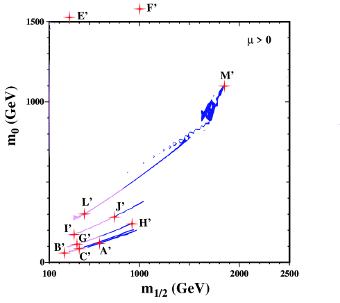
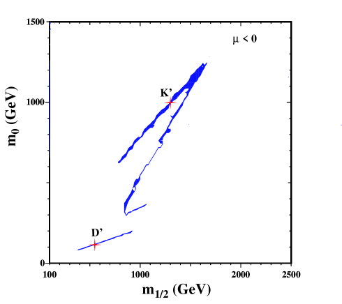
Figure 1: The shaded strips display the regions of the $(m_{1/2},m_{0})$ plane that are compatible [15] with $0.094<\Omega_{\chi}h^{2}<0.129$ in the ‘bulk’, coannihilation ‘tail’, and rapid-annihilation ‘funnel’ regions, as well as the laboratory constraints, for (a) $\mu>0$ and $\tan\beta=5,10,20,35$ and 50, and (b) for $\mu<0$ and $\tan\beta=10$ and 35. The parts of these ‘WMAP lines’ for $\mu>0$ compatible with $g_{\mu}-2$ at the 2-$\sigma$ level have lighter (pink) shading [7]. The updated post-WMAP benchmark scenarios are marked in red. Points (E’,F’) in the focus-point region have larger values of $m_{0}$.

We see also in Fig. 1 that the majority of the benchmark points lie on the portions of the WMAP lines with lower values of $m_{1/2}$, making them more interesting for the early stages of LHC operation, and for any sub-TeV linear $e^{+}e^{-}$ collider. Generally speaking, less fine-tuning of parameters is required in this region than in the focus-point, funnel and tail regions [32]: see also the discussion in [3].

2.2 Discussion of Spectra

In order to study the detectability of MSSM particles and the possible accuracies in measurements for the proposed benchmarks, it is essential to relate the input CMSSM parameters, defined in Table 1 for the SSARD program, to those necessary to obtain an equivalent MSSM spectrum in Monte Carlo generators . Accordingly, we have tuned the inputs for ISASUGRA 7.67 to reproduce as accurately as possible the spectra given in Table 1, by scanning $m_{0}$ and $\tan\beta$ to identify the parameter pairs minimizing the sum of the relative differences of particle masses $|m_{\tt SSARD}-m_{\tt ISASUSY}|/M_{\tt SSARD}$. In view of their importances for the calculation of $\Omega_{\chi}h^{2}$, we have treated specially the mass splitting $|m_{\tilde{\tau}_{1}}-m_{\chi}|$, which is important along the coannihilation ‘tail’, and also $|m_{A}-2m_{\chi}|$, where it becomes important in the ‘funnel’ regions. We have given each of them 30 % of the total weighting when optimizing the Isasugra 7.67 parameters in the relevant $(m_{1/2},m_{0})$ regions. The results of the optimization are given in Table 2.

Supersymmetric spectra in post-WMAP benchmarks
calculated with ISASUGRA 7.67
 
Model A’ B’ C’ D’ E’ F’ G’ H’ I’ J’ K’ L’ M’ $m_{1/2}$ 600 250 400 525 300 1000 375 935 350 750 1300 450 1840 $m_{0}$ 107 57 80 101 1532 3440 113 244 181 299 1001 303 1125 $\tan{\beta}$ 5 10 10 10 10 10 20 20 35 35 46 47 51 sign($\mu$) $+$ $+$ $+$ $-$ $+$ $+$ $+$ $+$ $+$ $+$ $-$ $+$ $+$ $m_{t}$ 175 175 175 175 171 171 175 175 175 175 175 175 175 Masses $|\mu(m_{Z})|$ 773 339 519 663 217 606 485 1092 452 891 1420 563 1940 h 116 113 117 117 114 118 117 122 117 121 123 118 124 H 896 376 584 750 1544 3525 525 1214 444 888 1161 480 1623 A 889 373 580 745 1534 3502 522 1206 441 882 1153 477 1613 H^± 899 384 589 754 1546 3524 532 1217 453 892 1164 490 1627 $\chi$ 242 95 158 212 112 421 148 388 138 309 554 181 794 $\chi_{2}$ 471 180 305 415 184 610 286 750 266 598 1064 351 1513 $\chi_{3}$ 778 345 525 671 229 622 492 1100 459 899 1430 568 1952 $\chi_{4}$ 792 366 540 678 302 858 507 1109 475 908 1437 582 1959 $\chi^{\pm}_{1}$ 469 178 304 415 175 613 285 750 265 598 1064 350 1514 $\chi^{\pm}_{2}$ 791 366 541 679 304 846 507 1108 475 908 1435 582 1956 $\tilde{g}$ 1367 611 940 1208 800 2364 887 2061 835 1680 2820 1055 3884 $e_{L}$, $\mu_{L}$ 425 188 290 376 1543 3499 285 679 304 591 1324 434 1660 $e_{R}$, $\mu_{R}$ 251 117 174 224 1534 3454 185 426 227 410 1109 348 1312 $\nu_{e}$, $\nu_{\mu}$ 412 167 274 362 1539 3492 270 665 290 579 1315 423 1648 $\tau_{1}$ 249 109 167 217 1521 3427 157 391 150 312 896 194 796 $\tau_{2}$ 425 191 291 376 1534 3485 290 674 312 579 1251 420 1504 $\nu_{\tau}$ 411 167 273 360 1532 3478 266 657 278 558 1239 387 1492 $u_{L}$, $c_{L}$ 1248 558 859 1103 1639 3923 814 1885 778 1554 2722 1001 3670 $u_{R}$, $c_{R}$ 1202 542 830 1064 1637 3897 787 1812 754 1497 2627 969 3528 $d_{L}$, $s_{L}$ 1250 564 863 1107 1641 3924 818 1887 783 1556 2723 1004 3671 $d_{R}$, $s_{R}$ 1197 541 828 1059 1638 3894 786 1804 752 1491 2615 967 3509 $t_{1}$ 958 411 653 860 1052 2647 617 1477 584 1207 2095 753 2857 $t_{2}$ 1184 576 837 1048 1387 3373 792 1753 748 1428 2366 920 3231 $b_{1}$ 1147 514 789 1015 1375 3356 737 1719 677 1377 2297 844 3149 $b_{2}$ 1181 535 816 1043 1602 3816 770 1761 725 1423 2349 904 3217

Table 2: Proposed post-WMAP CMSSM benchmark points and mass spectra (in GeV), as calculated using ISASUGRA 7.67 [20] and adapting the values of $m_{0}$ and $\tan\beta$ (when it is large) to give the best fit to the SSARD spectra shown in Table 1, as described in the text.

In general, good matching between the predictions of the two codes can be found with only moderate shifts of the input parameters, and we have chosen only to adjust $m_{0}$ in most cases. The typical average relative difference in the benchmark point masses is of the order of a few percent. However, occasionally individual masses may exhibit discrepancies of up to 15%, and ensuring compatible mass splittings $\Delta M$ requires a systematic shift in $m_{0}$ to higher values, particularly at large $\tan\beta$, as seen in Fig. 2, where the cases $\tan\beta=5,10,20,35$ and 50 are exhibited for $\mu>0$, and $\tan\beta=10$ for $\mu>0$. In addition to increasing $m_{0}$, here we find a better correspondence between SSARD and ISASUGRA 7.67 if $\tan\beta$ is allowed to be reduced, as done for benchmarks (K, L, M) in Table 2.

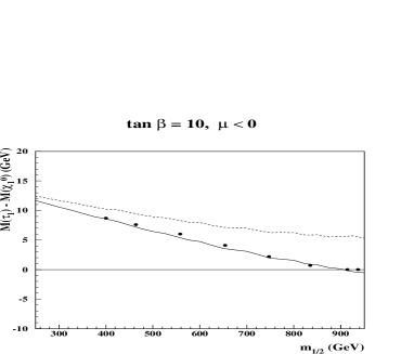
Figure 2: Comparison of the mass differences $\Delta M\equiv|m_{\tilde{\tau}_{1}}-m_{\chi}|$ along the WMAP lines, as calculated in the SSARD code (dots) and ISASUGRA 7.67 using the same values of $m_{0}$ (dashed lines), as functions of $m_{1/2}$ for $\mu>0$ and $\tan\beta=5,10,20,35,50$ and $\mu<0,\tan\beta=10$. We see the need to shift $m_{0}$ systematically, particularly at larger $m_{1/2}$ and $\tan\beta$. This has been done for the solid lines, which are improved ISASUGRA 7.67 fits to the WMAP lines described in the text.

We have further studied whether the resulting ISASUGRA 7.67 versions of the benchmark points yield values of $\Omega_{\chi}h^{2}$ that are indeed compatible with the WMAP data. The first line of Table 3 shows the values of $\Omega_{\chi}h^{2}$ calculated using the SSARD [18] code at the updated benchmark points shown in Table 1, which are well within the WMAP range. The second line shows the corresponding values of $\Omega_{\chi}h^{2}$ calculated using the Micromegas code [33] interfaced with the ISASUGRA 7.67 code that is used to calculate the spectra in Table 2. The agreement between SSARD and Micromegas/ISASUGRA 7.67 is generally good in the bulk and coannihilation tail regions, with the latter falling within the WMAP range, except for point H (which is right at the tip of the coannihilation tail) and point J (where the discrepancy is only marginal). The Micromegas/ISASUGRA 7.67 code gives results that are outside the WMAP range in the focus-point and at the upper edge of the funnel region (points E, F and M), reflecting the fact that the calculation of $\Omega_{\chi}h^{2}$ is notoriously delicate in these regions [32] and that the tuning of the mass spectra between the two different codes becomes difficult.

Relic density $\Omega_{\chi}h^{2},b\to s\gamma$ and $g_{\mu}-2$ in post-WMAP benchmark scenarios
 
A’ B’ C’ D’ E’ F’ G’ H’ I’ J’ K’ L’ M’ $\Omega_{\chi}h^{2}$: SSARD .12 .12 .12 .10 .10 .10 .13 .13 .12 .10 .10 .10 .14 $\Omega_{\chi}h^{2}$: Micromegas .09 .12 .12 .09 .33 2.56 .12 .16 .12 .08 0.12 .11 0.27 BR($b\to s\gamma$) $\times 10^{4}$ 3.9 3.1 3.8 4.5 3.7 3.7 3.3 3.6 2.5 3.4 4.2 2.5 3.5 $\delta a_{\mu}$ $\times 10^{9}$ 0.3 3.2 1.3 -0.8 0.2 0.03 2.7 0.4 4.5 1.1 -0.3 3.4 0.3

Table 3: Comparison of $\Omega_{\chi}h^{2}$ for the benchmark points in Table 1 computed with the SSARD code [18] (top line), and the Micromegas code [33] interfaced with ISASUGRA 7.67 [20] (second line) using the fitted parameters shown in Table 2. The third and fourth lines show the values of $b\to s\gamma$ and $g_{\mu}-2$ calculated using SSARD.

For completeness, we also present in Table 2 the values of the $b\to s\gamma$ branching ratio and the supersymmetric contribution to $g_{\mu}-2$ calculated using SSARD. These may be compared with any evolution in the future experimental values of these quantities. As already mentioned, the situation with regard to any possible non-Standard Model contribution to the experimental value of $g_{\mu}-2$ is sufficiently volatile that we do not use this as a criterion for selecting benchmarks, though it is used in Fig. 3 to order the benchmark points, as described below.

2.3 Observability at Different Accelerators

As an important ingredient in the subsequent analyses of sparticle observability at different colliders, we first report a comparison of the principal sparticle branching ratios at the updated benchmark points with those found previously [3] at the original benchmark points. The new branching ratios have been calculated using ISASUGRA 7.67, whereas previously they were calculated using ISASUGRA 7.51 [20], and we comment on the differences associated with the improvement in ISASUGRA, as opposed to the changes in the benchmark parameter choices . Since the differences in branching ratios are not large, in general, we limit ourselves to commenting on instances where the more significant differences occur.

$\bullet$ In the case of point A, the most notable difference is an increase in $B({\tilde{b}_{2}}\to b\chi)$ from 39 to 62 %, with corresponding decreases in $B({\tilde{b}_{2}}\to t+\chi^{-},{\tilde{t}_{1}}+W^{-})$. There is also an increase of $\chi_{4}\to h\chi_{2}$ from 23 to 29 % at the expense of $\chi_{4}\to W\chi^{\pm}_{1}$. These changes are not related to the new parameter choice, but to the differences in the ISASUGRA versions.

$\bullet$ In the case of point B, there is again an increase in $B({\tilde{b}_{2}}\to b\chi)$, from 15 to 25 %, and a decrease in $B({\tilde{b}_{2}}\to{\tilde{t}_{1}}+W^{-})$. There is also an increase in $B({\tilde{e}_{L}}\to e\chi)$ from 47 to 87 %, accompanied by decreases in $B({\tilde{e}_{L}}\to e\chi_{2},\nu+\chi^{\pm}_{1})$. We also note that the $B({\tilde{\nu}}_{\ell}\to\ell^{-}\chi^{+})$ now vanish, so that the ${\tilde{\nu}}_{\ell}$ are invisible. There is also an increase in $B({\tilde{\tau}}_{2}\to\tau\chi)$ from 51 to 84 %, which decreases $B({\tilde{\tau}}_{2}\to\nu_{\tau}+\chi^{-},\tau+\chi_{2})$. Finally, there are decreases in $B(\chi_{2}\to{\tilde{\tau}}_{1}+\tau)$ from 84 to 42 %, which increases the branching ratio for the invisible channel $B(\chi_{2}\to{\tilde{\nu}}+\nu)$, and in $B(\chi^{\pm}\to{\tilde{\tau}}_{1}+\nu_{\tau})$ from 96 to 36 %, which increases $B(\chi^{\pm}\to{\tilde{\nu}}+\ell)$. The changes for the sleptons are mostly because they are lighter at the updated benchmark point with smaller $m_{0}$, and those for $\tilde{b}_{2}$ are related to the differences in the ISASUGRA versions. Both effects influence the gaugino branching ratios.

$\bullet$ At benchmarks C and D, $B({\tilde{b}_{2}}\to b\chi)$ increases from 13 to 24 % and from 20 to 44 %, respectively, with corresponding decreases in $B({\tilde{b}_{2}}\to{\tilde{t}_{1}}W^{-})$ and $B({\tilde{b}_{2}}\to t+\chi^{\pm})$. At point C, decreases are observed of $\chi_{2}\to\widetilde{\tau}_{1}\tau$ from 23 to 13 % and of $\chi^{\pm}_{1}\to\widetilde{\tau}_{1}\nu$ from 21 to 11 %, compensated by increases of $\chi_{2}\to\widetilde{\nu}\nu$ and $\chi^{\pm}_{1}\to\widetilde{\nu}l$, respectively. All changes are mostly related to differences in the ISASUGRA versions.

$\bullet$ At the updated points E and F, the most notable effect is an increase of the branching ratios of squarks to gluinos, due to the increase in $m_{0}$ and hence of the squark masses at the updated benchmark points. For instance, the $B(\widetilde{b}_{1}\to b\tilde{g})$ changes from 45 to 52 % at E and from 22 to 38 % at F. They are compensated by a reduction of the decays to charginos and neutralinos. Moreover, at point E the decays of sleptons into $\chi^{\pm}_{1}$ tend to decrease and those into $\chi^{\pm}_{2}$ to increase correspondingly.

$\bullet$ At the updated benchmark G, there are increases in $B({\tilde{b}_{1}}\to t\chi^{\pm}_{2})$, from 13 to 22 %, with accompanying decreases in other modes, mainly in $B({\tilde{b}_{1}}\to t+\chi^{\pm}_{1},b+\chi_{2})$. A decrease is observed of $\chi_{2}\to\widetilde{\tau}_{1}\tau$ from 82 to 62 % and of $\chi^{\pm}_{1}\to\widetilde{\tau}_{1}\nu$ from 81 to 57 %, compensated by an increase of $\chi_{2}\to\widetilde{\nu}\nu$ and $\chi^{\pm}_{1}\to\widetilde{\nu}l$, respectively. The changes are mostly due to the differences in the ISASUGRA versions.

$\bullet$ Although the updated point H has a significantly lighter spectrum than previously, no major changes ($>$ 5-6 %) are observed in the decay branching ratios.

$\bullet$ For the old point I the decay $\widetilde{b}_{1}\to t\chi^{\pm}_{2}$ was kinematically forbidden. For the updated point it is allowed and has a branching ratio of 11 %. Also, $B(\widetilde{\nu}_{e}\to\nu\chi)$ increases from 61 to 73 % and $B(\widetilde{\nu}_{e}\to e\chi^{\pm}_{1})$ decreases correspondingly, mostly due to the change in the ISASUGRA version used.

$\bullet$ At point J the main changes are a decrease of $B(\chi_{2}\to\widetilde{\tau}_{1}\tau)$ from 82 to 66 % and of $B(\chi^{\pm}_{1}\to\widetilde{\tau}_{1}\nu)$ from 82 to 64 %, mostly compensated by an increase of $B(\chi_{2}\to\widetilde{\nu}\nu)$ and $B(\chi^{\pm}_{1}\to\widetilde{\nu}l)$, respectively. The changes are mainly due to the differences in the ISASUGRA versions.

$\bullet$ At the updated benchmark K, there is an increased branching ratio for the direct decay of ${\widetilde{e}}_{L}$ and $\widetilde{\nu}_{e}$ to $\chi$ from 26 to 35 % and 27 to 37 % respectively, at the expense of the decays to $\chi^{\pm}_{1}$. The increase of $B(\widetilde{\nu}_{\tau}\to W\widetilde{\tau}_{1})$ from 28 to 40 % is accompanied by a decrease of $B(\widetilde{\nu}_{\tau}\to\tau\chi^{\pm}_{1})$. Also, the decays of $\chi_{2}$ and $\chi^{\pm}_{1}$ to $\widetilde{\tau}_{1}$, which were previously forbidden kinematically, are now allowed by the new parameter values and reach 43 and 41 %, respectively. A reduction of $B(\chi_{4}\to W\chi^{\pm}_{1})$ from 56 to 47 % is also observed, associated with the differences in the ISASUGRA versions.

$\bullet$ The updated point L is characterized by a decrease of the branching ratios of $\widetilde{\nu}_{e}$ and $\widetilde{\nu}_{\tau}$ to the $\chi^{\pm}_{1}$, compensated by an increase of $B(\widetilde{\nu}_{e}\to\nu\chi)$ from 35 to 43 % and of $B(\widetilde{\nu}_{\tau}\to W\widetilde{\tau}_{1})$ from 59 to 77 %. The decay branching ratios of $\chi_{3}$ and $\chi_{4}$ to $\widetilde{\tau}_{1}\tau$ are increased from 19 to 27 % and 13 to 20 %, respectively, with a corresponding reduction of the decays to $\chi^{\pm}_{1}$. These changes are associated with the updated CMSSM parameter values.

$\bullet$ At the updated point M, the main change is a smaller value of $m_{0}$, which affects many branching fractions. We only mention some of the major changes. The direct decay to $\chi$ is increased for ${\widetilde{e}}_{L}$ and $\widetilde{\nu}_{e}$ from 34 to 74 % and from 34 to 77 %, repectively, at the expense of a reduced decay to the chargino and the heavier neutralino. The $B(\chi_{2}\to h+\chi)$ decreases from 45 to 12 %, whereas $B(\chi_{2}\to{\tilde{\tau}_{1}}+\tau)$ increases, and $B(\chi^{\pm}_{1}\to W^{\pm}+\chi)$ decreases from 48 to 14 %, whereas $B(\chi^{\pm}_{1}\to{\tilde{\tau}_{1}}+\nu_{\tau})$ increases.

The branching ratios at the updated benchmark points not mentioned above are not significantly different from those at the original versions of the points. Among all the above effects, perhaps the most significant is the invisibility of the ${\tilde{\nu}_{\ell}}$ at the updated version of point B.

Combining the above information, we now present in Fig. 3 an updated comparison of the numbers of different MSSM particles that should be observable at different accelerators in the various benchmark scenarios [3], ordered by their consistency with $g_{\mu}-2$ as calculated using $e^{+}e^{-}$ data for the Standard Model contribution [7]. We re-emphasize that the qualities of the prospective sparticle observations at hadron colliders and linear $e^{+}e^{-}$ colliders are often very different, with the latters’ clean experimental environments providing prospects for measurements with better precision. Nevertheless, Fig. 3 already restates the clear message that hadron colliders and linear $e^{+}e^{-}$ colliders are largely complementary in the classes of particles that they can see, with the former offering good prospects for strongly-interacting sparticles such as squarks and gluinos, and the latter excelling for weakly-interacting sparticles such as charginos, neutralinos and sleptons. We discuss later the detailed criteria used for assessing the detectabilities of different particles at different colliders.

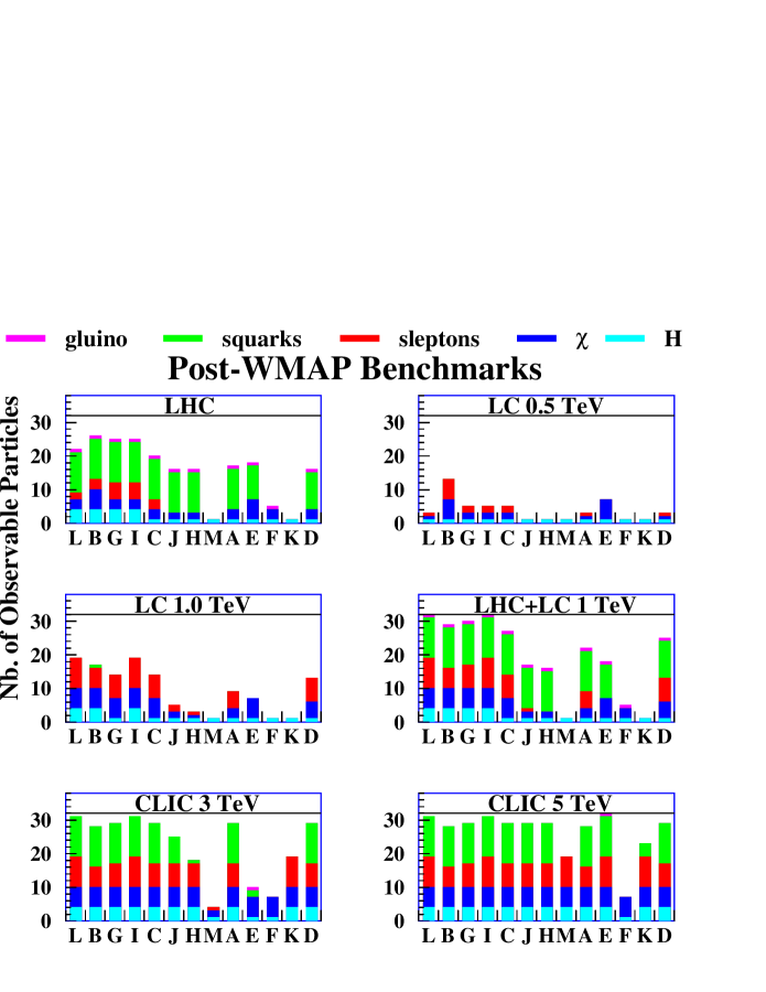
Figure 3: Summary of the numbers of MSSM particles that may be detectable at various accelerators in the updated benchmark scenarios. As in [3], we see that the capabilities of the LHC and of linear $e^{+}e^{-}$ colliders are largely complementary. We re-emphasize that mass and coupling measurements at $e^{+}e^{-}$ colliders are usually much cleaner and more precise than at hadron-hadron colliders such as the LHC, where, for example, it is not known how to distinguish the light squark flavours.

3 WMAP Lines

As has already been mentioned, in view of the reduction in dimensionality of the CMSSM parameter space enforced by WMAP [15], one may progress beyond the previous approach of sampling, more or less sparsely, the CMSSM parameter space. In particular, as proposed in [8] but with a different attitude towards the cosmological density constraint, one may explore, more or less systematically, the CMSSM phenomenology along the lines in parameter space shown in Fig. 1. Again as proposed in [8], one may then focus special attention on particular points along these lines. The updated benchmark points discussed in the previous section are examples and, as we discuss below, they manifest some of the distinctive possibilities that may appear along the WMAP lines. However, for certain purposes it may be helpful to select a few additional points that exemplify other generic possibilities, as we discuss later.

3.1 Parametrizations of WMAP Lines

As seen in Fig. 1, the WMAP lines have a relatively simple form for $\tan\beta\mathrel{\hbox to0.0pt{\raise 2.15277pt\hbox{$<$}\hss}{\lower 2.15277pt\hbox{$\sim$}}}35$. It is therefore possible to provide simple quadratic parametrizations for them that are a convenient summaries of the correlations between $m_{1/2}$ and $m_{0}$ that are enforced by WMAP within the CMSSM framework adopted here. Using the SSARD code, we find the following convenient parametrizations for the $\mu>0$ lines:

$$\tan\beta=~{}5:\; m_{0} \;=\;-5.46+0.206m_{1/2}+4.02\times 10^{-6}m_{1/2}^{2},\;(475\leq m_{1/2}\leq 960)$$ (2)

$$\tan\beta=10:\; m_{0} \;=\;11.97+0.163m_{1/2}+4.90\times 10^{-5}m_{1/2}^{2},\;(300\leq m_{1/2}\leq 940)$$ (3)

$$\tan\beta=20:\; m_{0} \;=\;50.89+0.144m_{1/2}+6.77\times 10^{-5}m_{1/2}^{2},\;(270\leq m_{1/2}\leq 940),$$ (4)

$$\tan\beta=35:\; m_{0} \;=\;90.24+0.219m_{1/2}+5.70\times 10^{-5}m_{1/2}^{2},\;(315\leq m_{1/2}\leq 1070)$$ (5)

where the masses are expressed in units of GeV, and the numbers in parentheses specify the allowed ranges of $m_{1/2}$. When $\tan\beta=50$, a rapid-annihilation funnel appears, and parametrizing the regions allowed by WMAP becomes more complicated. In the case of $\tan\beta=50$, one may conveniently use:

$$m_{0}\; = \;140.6+0.33m_{1/2}+6.3\times 10^{-5}m_{1/2}^{2}\;(350\leq m_{1/2}\leq 1550),$$

$$m_{0}\; = \;-1941+1.65m_{1/2}\;(1700\leq m_{1/2}\leq 1800),$$ (6)

where the masses are again expressed in GeV units. For $\mu<0$, we propose the following convenient parametrizations:

$$\tan\beta=10:\; m_{0} \;=\;15.0+0.16m_{1/2}+4.2\times 10^{-5}m_{1/2}^{2},\;(400\leq m_{1/2}\leq 940)$$ (7)

$$\tan\beta=35:\; m_{0} \;=\;39.6+0.76m_{1/2}-1.9\times 10^{-5}m_{1/2}^{2},\;(790\leq m_{1/2}\leq 1650),$$ (8)

where for $\tan\beta=35$ we parametrize only the top branch allowed by WMAP in the $(m_{1/2},m_{0})$ plane shown in panel (b) of Fig. 1, which includes the updated point K.

As mentioned earlier when discussing the specific benchmark points, the appropriate values of $m_{0}$ as functions of $m_{1/2}$ must be re-evaluated for the ISASUGRA 7.67 code. A similar minimization procedure to that discussed earlier has been repeated, parametrizing the shifts w.r.t. the values obtained with the SSARD code by a linear function of $m_{1/2}$, which have then been added to (5, 6, 8). The resulting parametrizations are:

$$\tan\beta=~{}5:\; m_{0} \;=\;-9.96+0.197m_{1/2}+4.02\times 10^{-6}m_{1/2}^{2},\;(475\leq m_{1/2}\leq 960)$$ (9)

$$\tan\beta=10:\; m_{0} \;=\;13.57+0.142m_{1/2}+4.90\times 10^{-5}m_{1/2}^{2},\;(300\leq m_{1/2}\leq 940)$$ (10)

$$\tan\beta=20:\; m_{0} \;=\;50.39+0.142m_{1/2}+6.77\times 10^{-5}m_{1/2}^{2},\;(270\leq m_{1/2}\leq 940),$$ (11)

$$\tan\beta=35:\; m_{0} \;=\;89.56+0.239m_{1/2}+5.70\times 10^{-5}m_{1/2}^{2},\;(300\leq m_{1/2}\leq 1050).$$ (12)

These have been used to produce the solid lines in Fig. 2.

We note in passing that, as the mass difference $\Delta M\equiv|m_{\tilde{\tau}_{1}}-m_{\chi}|\to 0$ towards the high-$m_{1/2}$ ends of the WMAP lines, these have portions at high $m_{1/2}$ where $\Delta M<m_{\tau}$. In these portions, the ${\tilde{\tau}_{1}}$ NLSP decays via a virtual $\tau$, resulting in the dominance of four-body decay modes such as ${\tilde{\tau}_{1}}\to\nu\chi\ell{\bar{\nu}}$ and $\nu\chi q{\bar{q}}$. In this case, the ${\tilde{\tau}_{1}}$ is stable on the scale of the size of the detector. This observation has important implications for ${\tilde{\tau}_{1}}$ observability at different colliders, as we discuss below.

3.2 Discussion of $\chi_{2}$ Decay Branching Ratios

One of the key particles appearing in sparticle decay chains is the second neutralino $\chi_{2}$, whose branching ratios are quite model-dependent and have significant impact on sparticle detectability at future colliders. Moreover, $\chi_{2}$ decays play crucial roles in reconstructing sparticle masses via cascade decays. Therefore, we now use ISASUGRA 7.67 to discuss how the principal branching ratios of the $\chi_{2}$ vary along the WMAP lines, noting several significant features that are important for phenomenology.

As seen in Fig 4(a) for $\tan\beta=5$ and $\mu>0$, $\chi_{2}$ decays into ${\tilde{\tau}}\tau$ and other ${\tilde{\ell}}\ell$ modes dominate among the decay modes of interest. Both ${\tilde{\tau}_{1}}\tau$ and ${\tilde{\tau}_{2}}\tau$ contribute, the latter increasing with $m_{1/2}$ while the former decreases. The dip in the the ${\tilde{\ell}}\ell$ branching ratio when $m_{1/2}\sim 300$ GeV reflects a similar switch between the ${\tilde{\ell}_{R}}\ell$ modes at low $m_{1/2}$ and the ${\tilde{\ell}_{L}}\ell$ modes at large $m_{1/2}$ . The most important other decay modes are the invisible $\chi_{2}\to{\tilde{\nu}}\nu$ decays. The decay modes $\chi_{2}\to\chi Z$ and $\chi_{2}\to\chi h$ exhibit clear thresholds at $m_{1/2}\sim 270$ GeV and 310 GeV, respectively, reflecting the opening up of these two channels. We note that benchmark A is in the region of $m_{1/2}$ where the branching ratio for $\chi_{2}\to\chi h$ is already declining from its peak value $\simeq 6$ %, while that for $\chi_{2}\to\chi Z$ has already been reduced from its peak value $\simeq 0.6$ %.

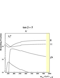
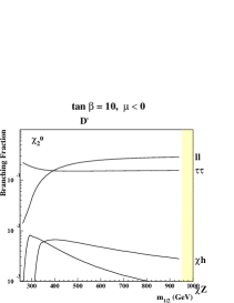
Figure 4: Dominant branching ratios of the next-to-lightest neutralino $\chi_{2}$ as functions of $m_{1/2}$ along the WMAP lines for (a) $\tan\beta=5$, (b) $\tan\beta=10$, (c) $\tan\beta=20$, (d) $\tan\beta=35$ and (e) $\tan\beta=50$, all for $\mu>0$, and (f) $\tan\beta=10$ for $\mu<0$. The locations of updated benchmark points along these WMAP lines are indicated, as are the upper limits on $m_{1/2}$ in panels (a, b, c) and (f).

Similar features are exhibited in Fig 4(b) for $\tan\beta=10$ and $\mu>0$, with the peak in the branching ratio for $\chi_{2}\to\chi h$ reduced to $\simeq 5$ % and that for $\chi_{2}\to\chi Z$ increased to $\simeq 0.9$ %. The updated benchmark point B with $m_{1/2}=250$ GeV is below both thresholds, whilst benchmark C has a near-maximal branching ratio for $\chi_{2}\to\chi h$.

Panel (c) of Fig. 4 shows the corresponding $\chi_{2}$ decay branching ratios for $\tan\beta=20$ and $\mu>0$. We see that the ${\tilde{\tau}}\tau$ mode is larger than for $\tan\beta=10$, reflecting the larger $\tau$ Yukawa coupling. The dip in the ${\tilde{\ell}}\ell$ has moved to larger $m_{1/2}\sim 400$ GeV. The thresholds in $\chi_{2}\to\chi Z$ and $\chi_{2}\to\chi h$ are again prominent, with the former branching ratio now reaching slightly more than 1 %. Benchmark G is located near the peak in $\chi_{2}\to\chi h$ and the dip in $\chi_{2}\to{\tilde{\ell}}\ell$, whilst benchmark H has almost equal branching ratios for ${\tilde{\ell}}\ell$ and ${\tilde{\tau}}\tau$, and smaller branching ratios for $\chi h$ and particularly $\chi Z$.

When $\tan\beta=35$ and $\mu>0$, shown in panel (d) of Fig. 4, $\chi_{2}\to{\tilde{\tau}}\tau$ becomes the dominant branching ratio for all values of $m_{1/2}$ allowed by WMAP. Apart from this, the most noticeable feature is the relative suppression of the $\chi_{2}\to{\tilde{\ell}}\ell$ branching ratio, whose dip has now moved up to $m_{1/2}\sim 700$ GeV. The branching ratio for $\chi_{2}\to\chi h$ exhibits a broad peak of similar height to the lower values of $\tan\beta$, whereas the branching ratio for $\chi_{2}\to\chi Z$ is somewhat smaller. Benchmark I is located near the peaks of the $\chi_{2}\to\chi h,\chi Z$ branching ratios, and benchmark J is located in the region of $m_{1/2}$ where the $\chi_{2}\to{\tilde{\ell}}\ell$ starts to rise.

Panel (e) of Fig. 4 shows the branching ratios for $\tan\beta=50$ and $\mu>0$. Here we note the strong dominance of $\chi_{2}\to{\tilde{\tau}}\tau$ decays, the approximate constancies (at relatively low levels) of the branching ratios for $\chi_{2}\to\chi h,Z$ above their respective thresholds, and the strong suppression of $\chi_{2}\to{\tilde{\ell}}\ell$ decays. Benchmark L has branching ratios that are typical for this value of $\tan\beta$.

Finally, panel (f) of Fig. 4 shows the branching ratios for $\tan\beta=10$ when $\mu<0$. In this case, there is dip structure in the branching ratio for $\chi_{2}\to{\tilde{\ell}}\ell$, which rises monotonically with $m_{1/2}$, while the branching ratio for $\chi_{2}\to{\tilde{\tau}}\tau$ is always large. In this case, the peak branching ratio for $\chi_{2}\to\chi h$ is below that for $\chi_{2}\to\chi Z$.

The $\chi_{2}$ branching ratios are rather different at the tip of the funnel for $\tan\beta=50$ - which has BR($\chi_{2}\to\chi h$) = 0.11 at the location of point M, by point K on the side of the rapid-annihilation funnel for $\tan\beta=35$ and $\mu<0$ - where the mode $\chi_{2}\to\chi h$ gives half of the total $\chi_{2}$ decay rate, and at the focus points E and F - where the $\chi_{2}$ decay rate is saturated by $\chi q\bar{q}$ and by $\chi h$, respectively.

4 Production and Detectability along WMAP lines

We now study the reaches at different accelerators in the number of observable supersymmetric particles, and the changes in experimental signatures and topologies along the WMAP lines for different values of $\tan\beta$.

4.1 LHC

4.1.1 Sparticle Signatures

In order to visualize the changes in the signatures of sparticle decays along the WMAP lines, we first compute the mean numbers of different particle species produced in sparticle decay chains at LHC. Large samples of inclusive supersymmetric events have been generated along the WMAP lines, using PYTHIA 6.215 [34] interfaced to ISASUGRA 7.67 [20] to compute the average numbers of different particle species produced per supersymmetric event, and the production cross sections of exclusive and inclusive sparticle production reactions. Fig. 5 shows the average numbers of (a) $Z$, (b) $h$ bosons, (c) $\tau$ leptons and (d) trilepton events with three $\ell$ ($\ell=e,~{}\mu$) in inclusive sparticle decays at the LHC. The plots are all for $\mu>0$ and display results for $\tan\beta=10,20,35$ and 50 along the corresponding WMAP lines.

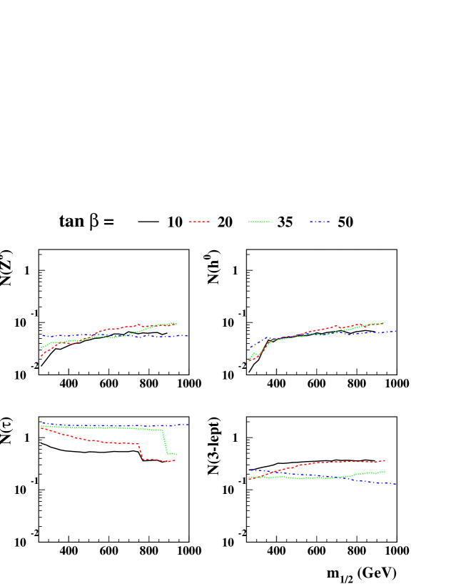
Figure 5: Supersymmetric event signatures at the LHC: the numbers of $Z$ bosons (upper left), light Higgs bosons $h$ (upper right), $\tau$ leptons (lower left) and three-lepton final states per supersymmetric event are shown as functions of $m_{1/2}$ along the WMAP lines for four values of $\tan\beta$, all with $\mu>0$. These plots were obtained with PYTHIA 6.215 [34] interfaced to ISASUGRA 7.67 [20].

We see in panel (a) of Fig. 5 that the fractions of sparticle decays with a $Z$ boson in the cascade is never large in the regions of the parameter space traversed by the WMAP lines, reaching about 0.1 $Z^{0}$/sparticle decay at large $m_{1/2}$ and $\tan\beta$.

The decays of sparticles into the lightest Higgs boson $h$, followed by $h\to b\bar{b}$ decay, provide another important signature at the LHC. These appear above the threshold for $\chi_{2}\to\chi h$ decay at about $m_{1/2}$=350 GeV, and may reach 7-10% per sparticle event at larger $m_{1/2}$, as seen in panel (b) of Fig. 5.

As seen in panel (c), the numbers of $\tau$ leptons produced in sparticle events are always large, particularly at large $\tan\beta$ where there are between one and two per event. Finally, we see in panel (d) of Fig. 5 that the fraction of trilepton events is always above 10%, and may attain $\sim 40$% at large $m_{1/2}$ and small $\tan\beta$.

These plots reinforce the importance of the $\tau$ signature for sparticle detection at the LHC, within the CMSSM framework used here. Clearly the $\chi_{2}\to\chi h,Z$ signatures are also interesting, but they may be quite challenging to exploit. However, we would like to emphasize that other decay patterns should not be neglected, and may be preferred in other supersymmetric models. For example, if the soft supersymmetry-breaking scalar masses for the Higgs multiplets are non-universal, $\chi_{2}\to\chi h,Z$ decays may be more copious.

4.1.2 Detectability at the LHC

We now estimate the numbers of different species of supersymmetric particles that may be detectable at the LHC as functions of $m_{1/2}$ along the WMAP lines for different values of $\tan\beta$, using the following criteria.

$\bullet$ Higgs bosons: We generally follow the ATLAS and CMS studies of the numbers of observable bosons as functions of $M_{A}$ and $\tan\beta$ [35]. In contrast to [3], here we also consider $H/A\to\chi_{2}\chi_{2}$ decays.

$\bullet$ Gauginos: Our criteria for the observability of heavier neutralinos at the LHC have been refined compared to our previous publication [3]. In particular, we first compute the total numbers of $\chi_{2}$ produced in all sparticle events and the branching fraction corresponding to a dilepton final state. We consider this to be observable at the LHC if the product is at least 0.01 pb, corresponding to 1000 events produced with 100 fb^-1 of integrated luminosity. The lightest neutralino $\chi$ is considered always to be detectable via the cascade decays of observed supersymmetric particles.

$\bullet$ Gluinos: These are considered to be observable for masses below 2.5 TeV [36].

$\bullet$ Squarks: The spartners of the lighter quark flavours $u,d,s,c$ are considered to be observable if $m_{\tilde{q}}<$ 2.5 TeV [36], but we recall that it is not known how to distinguish the spartners of different light-quark flavours at the LHC. In general, we assume that the stops and sbottoms ${\tilde{t}},{\tilde{b}}$ are observable only if they weigh below 1 TeV, unless the gluino weighs $<2.5$ TeV and the stop or sbottom can be produced in its two-body decays.

$\bullet$ Charged Sleptons: These are considered to be observable when the mass splitting $m_{\tilde{\ell}}-m_{\chi}>30$ GeV  and the inclusive production cross section, which includes their direct production and that in the decays of other supersymmetric particles, exceeds 0.1 pb, giving at least 10000 events with 100 fb^-1 of integrated luminosity .

$\bullet$ Sneutrinos: These have not been considered as observable at the LHC, due to their large yield of invisible $\tilde{\nu}\to\nu\chi$ decays.

We first note the key differences between the expected numbers of detectable MSSM particles at the updated benchmark points, shown in Fig. 3, and the analogous LHC analysis in [3]. Howver, we would like to caution the reader that it is impossible to be precie about the capabilities of the LHC (or other accelerator) without detailed simulations that go beyond the scope of this paper.

$\bullet$ At point B, we now consider the heavier neutral Higgs bosons to be detectable via their decays into the $\chi_{2}$ and into $\tau$ leptons, and the $H^{\pm}\to\tau\nu$ decays should also be detectable.

$\bullet$ We no longer consider the $H^{\pm}$ to be observable at point C.

$\bullet$ At point F, we now observe that the ${\tilde{g}}$ has branching ratios of 16 % and 17 %, respectively, for decays into $\chi_{2,3}{\bar{t}}t$, followed by branching ratios of 97 % and 99 % for $\chi_{2}\to\chi h$ and $\chi_{3}\to\chi Z$, respectively. The ${\tilde{g}}$ also has a branching ratio of 33 % for the decay into $\chi^{\pm}{\bar{t}}b$. We now consider that the $\chi_{2,3}$ should be detectable at this point, but not the $\chi^{\pm}$.

$\bullet$ At point H, supersymmetric particles are now well within the reach of the LHC, essentially because of the reduction in $m_{1/2}$. We now consider the ${\tilde{q}}$, ${\tilde{g}}$, $\chi$ and $\chi_{2}$ to be detectable at this point.

$\bullet$ At point J, we now consider the $\chi_{2}$ to be observable because of its large production rate, even though its decays generally include $\tau$ leptons.

$\bullet$ At point K, we now find that no sparticles are observable with our present criteria, although the lightest Higgs boson $h$ is observable.

A corollary of these changes is that supersymmetric particles appear to be detectable at the LHC at all the updated benchmark points except K and M, which are located in rapid-annihilation funnels.

We now display in Fig. 6, as functions of $m_{1/2}$ along the WMAP lines for different values of $\tan\beta$, the numbers of different types of MSSM particles that should be observable at the LHC with 100 fb^-1 of integrated luminosity in each of ATLAS and CMS. The nominal lower bounds on $m_{1/2}$ imposed by $m_{h}$ (dashed lines) and $b\to s\gamma$ (dot-dashed lines) are also shown. These each have some uncertainties, for example FeynHiggs has a quoted error of $\sim 2$ GeV in the calculation of $m_{h}$ so that (specifically) benchmark B in the top right panel should not be regarded as excluded.

Figure 6: Estimates of the numbers of MSSM particles that may be detectable at the LHC as functions of $m_{1/2}$ along the WMAP lines for $\mu>0$ and $\tan\beta=5,10,20,35$ and $50$, and for $\mu<0$ and $\tan\beta=10$. The locations of updated benchmark points along these WMAP lines are indicated, as are the nominal lower bounds on $m_{1/2}$ imposed by $m_{h}$ (dashed lines) and $b\to s\gamma$ (dot-dashed lines).

We use the criteria explained above and generalize the results for the indicated benchmark scenarios that were shown in Fig. 3. In the top left panel, for $\tan\beta=5$, we note first that only one MSSM Higgs boson is expected to be visible. In the top right panel for $\tan\beta=10$, we see that the other Higgs bosons are also expected to be observable at low $m_{1/2}$ in the neighbourhood of point B, for example via decays into $\chi_{2}\chi_{2}$. All of the Higgs bosons are expected to observable over the entire range of $m_{1/2}$ for $\tan\beta=35,50$ and $\mu>0$, but not for $\tan\beta=10$ and $\mu<0$ (bottom right panel). All of the charginos and neutralinos are expected to be observable at low $m_{1/2}$, but only the lightest neutralino $\chi$ at high $m_{1/2}$. Since the sneutrinos decay invisibly and the rates for ${\tilde{\ell}_{2}}$ production are inadequate, only the ${\tilde{\ell}_{1}}$ are considered to be observable at the LHC for this value of $\tan\beta$, and only at low $m_{1/2}$. However, all the squarks and gluinos are expected to be observable anywhere along any of the WMAP lines, except that for $\tan\beta=50$ and $\mu>0$, where sparticles would be unobservable at the end of the funnel, as exemplified by benchmark point M in Fig 3.

In the cases of larger values of $\tan\beta$, shown in the other panels of Fig. 6, all the MSSM Higgs bosons are expected to be observable for all the WMAP ranges of $m_{1/2}$. However, the observabilities of the different charginos and neutralinos resemble those for $\tan\beta=10$. Some of the ${\tilde{\ell}_{2}}$ may be observable, at least for small $m_{1/2}$. As for $\tan\beta=10$, all the squarks and gluinos are expected to observable at the LHC anywhere along the parts of the WMAP lines that are shown, with the exception of the tip of the line for $\tan\beta=50$.

We comment finally on the case of the metastable ${\tilde{\tau}_{1}}$ that appears towards the end of the WMAP lines where $\Delta M=|m_{\tilde{\tau}_{1}}-m_{\chi}|<m_{\tau}$. There is no specific study of this scenario at the LHC, but it has been estimated in an analogous gauge-mediated supersymmetry-breaking scenario that the efficiency for observing a metastable particle with $m=640$ GeV would be 25 % (increasing for larger masses), and that a signal should be detectable if the overall production cross-section exceeds 1 fb [37]. In view of the large sparticle production cross sections at the LHC, and the fact (see Fig. 5) that each sparticle event produces on average 0.1 or more ${\tilde{\tau}_{1}}$ particles per event towards the ends of the WMAP lines, we believe that a metastable ${\tilde{\tau}_{1}}$ could be detected out to the ends of the coannihilation tails. On the other hand, it may not be easy to determine the mass accurately, as the peak measured from the relativistic $1/\beta$ factor broadens with increasing mass. For example, when $m=640$ GeV the FWHM of the mass distribution is estimated to be about 250 GeV [37]. The error in the mass estimate may be reduced in a large statistical sample, but such an analysis would need to assume a realistic experimental environment in order to evaluate systematic errors.

4.2 Detectability at $e^{+}e^{-}$ Linear Colliders

Our criteria for the observability of supersymmetric particles at linear colliders are based on their pair-production cross sections.

$\bullet$ Particles with cross sections in excess of 0.1 fb are considered as observable, thanks to their production in more than 100 events with an integrated luminosity of 1 ab^-1.

$\bullet$ The lightest neutralino $\chi$ is considered to be observable only through its production in the decays of heavier supersymmetric particles.

$\bullet$ Sneutrinos are considered to be detectable when the sum of the branching fractions for decays which lead to clean experimental signatures, such as $\tilde{\nu}_{\ell}\to\chi^{\pm}\ell^{\mp}$ ($\ell$ = $e$, $\mu$, $\tau$) and $\tilde{\nu}_{\tau}\to W^{+}\tilde{\tau_{1}}^{-}$, exceeds 15%.

$\bullet$ The $\gamma\gamma$ collider option at a linear collider would allow one to produce heavy neutral Higgs bosons via the $s$-channel processes $\gamma\gamma\to A$ and $\gamma\gamma\to H$, extending the reach up to 750 GeV for 0.5 TeV $e^{\pm}$ beams and up to 1.5-2.0 TeV for 1.5 TeV $e^{\pm}$ beams. A $\gamma\gamma$ collider may also be used to look for gluinos, but we do not include this possibility in our analysis.

$\bullet$ Finally, we assume that a metastable ${\tilde{\tau}_{1}}$ could be detected at any linear $e^{+}e^{-}$ collider with more than 100 events, and note that the mass could be measured more accurately than at the LHC, by measuring the production threshold as well as $1/\beta$.

We consider $e^{+}e^{-}$ collision energies $\sqrt{s}$ = 0.5 TeV, 1.0 TeV, 3 TeV and 5 TeV, and also the combined capabilities of the LHC and a 1-TeV linear collider. Comparing our present estimates of the physics reaches of linear $e^{+}e^{-}$ colliders of different energies with those in [3], we observe changes due both to the criteria adopted and to the mass spectra. We note briefly the principal changes.

$\bullet$ The updated point F has no supersymmetric particles observable at 1 TeV centre-of-mass energy. This is in part due to differences in the ISAJET spectrum optimisation, where it now reproduces more closely that from SSARD.

$\bullet$ On the other hand, the reductions in the parameters $m_{1/2},m_{0}$ for point H make slepton-pair production possible already below 1 TeV. The same point now has one squark accessible at CLIC with centre-of-mass energy 3 TeV, and all of the squarks at 5 TeV.

$\bullet$ Point M now has no squarks accessible even to CLIC operating with a centre-of-mass energy of 5 TeV.

4.2.1 TeV-Class $e^{+}e^{-}$ Linear Colliders

The capabilities of a linear $e^{+}e^{-}$ collider with $\sqrt{s}$ = 0.5 TeV are illustrated in Fig. 7 [21]. It can see some gauginos and sleptons if $m_{1/2}\mathrel{\hbox to0.0pt{\raise 2.15277pt\hbox{$<$}\hss}{\lower 2.15277pt\hbox{$\sim$}}}500$ GeV. Its capabilities are therefore well suited to the $g_{\mu}-2$-friendlier scenarios displayed in the left columns of Fig. 3. Moreover, the sparticles that it would see would complement those detectable at the LHC. Also, we recall that such a linear collider would be able to measure sparticle properties much more accurately than the LHC [3, 8].

Figure 7: Estimates of the numbers of MSSM particles that may be detectable at a 0.5-TeV linear $e^{+}e^{-}$ collider as functions of $m_{1/2}$ along the WMAP lines for $\mu>0$ and $\tan\beta=5,10,20,35$ and $50$, and for $\mu<0$ and $\tan\beta=10$. The locations of updated benchmark points along these WMAP lines are indicated, as are the nominal lower bounds on $m_{1/2}$ imposed by $m_{h}$ (dashed lines) and $b\to s\gamma$ (dot-dashed lines).

A linear $e^{+}e^{-}$ collider able to deliver collisions at a centre of mass energy $\sqrt{s}=1$ TeV has the potential to complement significantly the LHC in studying the supersymmetric spectrum, as seen in Fig. 8. In particular, such a linear collider would observe most sleptons and gauginos as long as $m_{1/2}$ is below about 600 GeV, as exemplified by benchmarks B, C, G, I and L. Also, it would detect at least one supersymmetric particle over the whole range of the WMAP lines, even up to their upper $m_{1/2}$ limits exemplified by benchmark point H, except in the funnel cases: $\mu>0,\tan\beta=50$ and $\mu<0,\tan\beta=35$. The accuracy it would provide in the measurements of several sparticle masses would enable GUT mass relations to be tested, thereby completing the exploitation of the LHC data. We note also that a 1-TeV linear $e^{+}e^{-}$ collider would be able to observe the lightest squark, the ${\tilde{t}_{1}}$, at low values of $m_{1/2}$. This possibility is exemplified by benchmark point B, as also seen in Fig. 3.

Figure 8: Estimates of the numbers of MSSM particles that may be detectable at a 1-TeV linear $e^{+}e^{-}$ collider as functions of $m_{1/2}$ along the WMAP lines for $\mu>0$ and $\tan\beta=5,10,20,35$ and $50$, and for $\mu<0$ and $\tan\beta=10$. The locations of updated benchmark points along these WMAP lines are indicated, as are the nominal lower bounds on $m_{1/2}$ imposed by $m_{h}$ (dashed lines) and $b\to s\gamma$ (dot-dashed lines).

The complementarity between the LHC and 1-TeV linear $e^{+}e^{-}$ collider is displayed clearly in Fig. 9, where we see that, together, they cover the majority of the MSSM spectrum over most of the $m_{1/2}$ ranges covered by the different WMAP lines.

Figure 9: Estimates of the combined numbers of MSSM particles that may be detectable at a combination of the LHC and a 1-TeV linear $e^{+}e^{-}$ collider as functions of $m_{1/2}$ along the WMAP lines for $\mu>0$ and $\tan\beta=5,10,20,35$ and $50$, and for $\mu<0$ and $\tan\beta=10$. The locations of updated benchmark points along these WMAP lines are indicated, as are the nominal lower bounds on $m_{1/2}$ imposed by $m_{h}$ (dashed lines) and $b\to s\gamma$ (dot-dashed lines).

4.2.2 CLIC

A 3-TeV lepton collider, such as CLIC, is expected to access almost all the sparticle spectrum for $m_{1/2}<700$ GeV, as seen in Fig. 10. This would enable it, for example, to distinguish and provide detailed measurements of the different flavours of squarks that will not be possible at the LHC. Moreover, at larger $m_{1/2}$ CLIC would be able to observe (almost) all the spectrum of Higgs bosons, sleptons, charginos and neutralinos [23]. CLIC will also be able to observe gluinos via squark decays at the focus-point benchmark E . It would therefore provide full complementarity with the LHC along the full extension of the lines.

Figure 10: Estimates of the numbers of MSSM particles that may be detectable at the 3-TeV version of the CLIC linear $e^{+}e^{-}$ collider as functions of $m_{1/2}$ along the WMAP lines for $\mu>0$ and $\tan\beta=5,10,20,35$ and $50$, and for $\mu<0$ and $\tan\beta=10$. The locations of updated benchmark points along these WMAP lines are indicated, as are the nominal lower bounds on $m_{1/2}$ imposed by $m_{h}$ (dashed lines) and $b\to s\gamma$ (dot-dashed lines).

Finally, we display in Fig. 11 the capabilities of a 5-TeV lepton collider such as CLIC. We see that all the MSSM particles are detected along all the WMAP lines, with the exception of the gluino that would generally have been seen at the LHC, and, for $\mu>0$ and $\tan\beta=50$, squarks towards the tip of the corresponding WMAP line, including the point M.

Figure 11: Estimates of the numbers of MSSM particles that may be detectable at the 5-TeV version of the CLIC linear $e^{+}e^{-}$ collider as functions of $m_{1/2}$ along the WMAP lines for $\mu>0$ and $\tan\beta=5,10,20,35$ and $50$, and for $\mu<0$ and $\tan\beta=10$. The locations of updated benchmark points along these WMAP lines are indicated, as are the nominal lower bounds on $m_{1/2}$ imposed by $m_{h}$ (dashed lines) and $b\to s\gamma$ (dot-dashed lines).

Despite the larger machine-induced backgrounds and beam energy spread, CLIC is expected to perform measurements of the properties of accessible suspersymmetric particles with good accuracy [23]. Slepton and heavy Higgs boson masses can be determined to ${\cal{O}}$(1%) accuracy, also when accounting for realistic experimental conditions and resolutions. A similar accuracy can typically be obtained also for sparticles reconstructed through cascade decays, such as the the $\chi_{2}$ discussed below. The availability of polarized beams is not only beneficial to increase the signal cross sections (such as in the case of slepton-pair production) but also as an analyzing tool. A combination of measurements of the stop-pair production with different polarisation states can be used to determine the stop mixing angle [23].

4.3 A Neutralino Case Study

Many of the most interesting differences in the capabilities of the different colliders discussed above arise in the spectrum of charginos and neutralinos. In particular, while the LHC and a TeV-scale linear $e^{+}e^{-}$ collider are largely complementary, they may not be able to discover all the charginos, neutralinos and sleptons when $m_{1/2}\mathrel{\hbox to0.0pt{\raise 2.15277pt\hbox{$>$}\hss}{\lower 2.15277pt\hbox{$\sim$}}}400$ GeV, whereas CLIC can in principle observe all of them along all of the WMAP lines. To confirm these statements, we now compare the physics reaches of different accelerators for neutralinos in the $(m_{1/2},m_{0})$ plane, with the conclusions shown in Fig. 12(a).

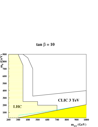
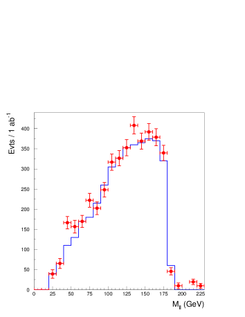
Figure 12: (a) Comparison of the sensitivities in the $(m_{1/2},m_{0})$ plane of the LHC and CLIC at 3 TeV to $\chi_{2}\to\chi\ell^{+}\ell^{-}$ decay and (b) the dilepton mass spectrum from this decay observable at 3-TeV CLIC for the CMSSM point $m_{1/2}=700$ GeV, $m_{0}=150$ GeV, $\mu>0$ and $\tan\beta=10$ discussed in the text.

For the LHC, we show Fig. 12(a) the region of the $(m_{1/2},m_{0})$ plane for $\tan\beta=10$ in which dilepton structures due to the decay chains $\chi_{2}\to\ell\tilde{\ell},\tilde{\ell}\to\ell\chi$ and $\chi_{2}\to XZ^{0},Z^{0}\to\ell^{+}\ell^{-}$ are expected to be observable in the cascade decays of heavier sparticles. We consider $\ell=e,\mu$ only, though the case $\ell=\tau$ would also be interesting at large $\tan\beta$, and require $\sigma\times$ dilepton branching ratio to exceed 0.01 pb, as discussed above. For our purposes, the relevant parts of the $(m_{1/2},m_{0})$ plane are those allowed by the WMAP dark matter constraint. We see that here the LHC coverage extends up to $m_{1/2}\simeq 500$ GeV, as also reflected in Fig. 6.

In order to see how accurately the 3-TeV version of CLIC could measure heavier neutralinos, we have made a new simulation of the process $e^{+}e^{-}\to\chi\chi_{2}$ followed by the decay chains $\chi_{2}\to\ell\tilde{\ell},\tilde{\ell}\to\ell\chi$ and $\chi_{2}\to XZ^{0},Z^{0}\to\ell^{+}\ell^{-}$, using SIMDET [38] to simulate the detector response and PYTHIA 6.215 [34] interfaced to ISASUGRA [20] to simulate the signal. Events with at least two leptons and significant missing energy were selected. Both slepton and Standard Model gauge-boson pair-production backgrounds were considered. Combinatorial backgrounds were subtracted by taking the difference of the pair $e^{+}e^{-}+\mu^{+}\mu^{-}$ events and the mixed $e^{\pm}\mu^{\mp}$ events, and a sliding window has been used to search for a $>$5-$\sigma$ excess in the $M_{\ell\ell}$ mass distribution. The results shown in Figure 12(a) for $\tan\beta=10$ make manifest the extended reach provided by CLIC, covering all the range of $m_{1/2}$ allowed by WMAP. At larger values of $\tan\beta$, decay chains involving the $\tilde{\tau}$ become more significant, requiring a more detailed study that should include $\tau$ reconstruction.

To benchmark the 3-TeV CLIC capabilities for measuring the masses of heavy neutralinos, a representative point has been chosen at $m_{1/2}=700$ GeV, $m_{0}=150$ GeV, $\mu>0$ and $\tan\beta=10$, along the corresponding WMAP line. Here, $m_{\chi_{2}}=540$ GeV, $m_{\chi}=290$ GeV and $m_{\ell_{L}}=490$ GeV. As seen in Fig. 12(b), at CLIC the dilepton invariant mass distribution shows a clear upper edge at 120 GeV due to $\chi_{2}\to\ell^{+}\tilde{\ell^{-}}_{L}$ followed by $\tilde{\ell^{-}}_{L}\to\ell^{-}\chi$, which can be very accurately measured with 1 ab^-1 of data. However, in order to extract the mass of the $\chi_{2}$ state, the masses of both the $\tilde{\ell}_{L}$ and $\chi$ need to be known. In fact, making a two-parameter fit to the muon energy distribution, the masses of the $\tilde{\mu}_{L}$ and $\chi$ can be extracted with an accuracy of 3 % and 2.5 %, respectively, with 1 ab^-1 of data [39]. Improved accuracy can be obtained with higher luminosity and using also a threshold energy scan. We therefore assume that these masses can be known to 1.7 % and 1.5 % respectively, which gives an uncertainty of 8 GeV, or 1.6 %, on the $\chi_{2}$ mass, accounting for correlations. This uncertainty is dominated by that in the $\tilde{\ell}$ and $\chi$ masses. The accuracy on the determination of the end point alone would correspond to a $\chi_{2}$ mass determination to 0.3 GeV, fixing all other masses, which is not sensitive to the details of the beamstrahlung and accelerator-induced backgrounds.

5 Conclusions

We have seen in this paper how different colliders could provide complementary information about the MSSM spectrum in updated CMSSM benchmark scenarios and along lines in the $(m_{1/2},m_{0})$ planes for different values of $\tan\beta$ and both signs of $\mu$. In addition to direct and indirect laboratory constraints, we have implemented the constraints on cold dark matter imposed by WMAP and other astrophysical and cosmological data.

We emphasize that the LSP is stable in any supersymmetric model in which $R$ parity is conserved, such as the MSSM, in which case astrophysical and cosmological constraints on dark matter must be taken into account. In principle, the LSP might be some different sparticle, such as the gravitino or axino. Specific scenarios of this type include models with gauge-mediated supersymmetry breaking, and benchmarks for such models have been proposed elsewhere [8]. We recall, however, that the WMAP data on reionization of the early Universe disfavour models with warm dark matter [12], so that all such models must grapple with the constraint on cold dark matter provided by WMAP and other data.

Alternatively, one might seek to avoid the cold dark matter constraints by postulating some amount of $R$ violation. The collider signatures of any such model would differ from those of the MSSM if $R$-violating couplings are not sufficiently small, and an additional set of astrophysical and cosmological constraints come into play if the $R$-violating couplings are not very large. Any $R$-violating scenario must address these issues.

We have updated a set of thirteen CMSSM benchmark points proposed previously [3] in light of the current WMAP constraint on supersymmetric dark matter. Since this constraint has reduced the dimensionality of the CMSSM parameter space, we have also introduced ‘WMAP lines’ in the $(m_{1/2},m_{0})$ plane for different values of $\tan\beta$, and have studied the physics reach of different accelerators, by charting the decay signatures and numbers of observable particles. It is interesting to observe that some important signatures, such as the pattern of $\chi_{2}$ decays, remain rather uniform along these lines. However, we note that different signatures may be recovered by relaxing some of the assumptions taken here. An interesting example is the appearence of large $\chi_{2}$ decay branching fractions into $h^{0}$ or $Z^{0}$ in models with non-universal Higgs masses. As these are of importance for defining the phenomenology of early runs at the LHC, we plan to consider them separately in conjunction with the corresponding dark matter density constraints.

The observation at the LHC of an excess of events containing large missing transverse energy could immediately indicate that supersymmetry is present, and that $R$ parity is conserved, so that the Universe should contain relic LSPs. However, it is possible that the relic LSP density might not saturate the bound on cold dark matter from WMAP, since there could be other significant contributions to the cold dark matter, e.g., from axions or superheavy metastable particles. It is therefore interesting and important to study, within the CMSSM framework considered here, to what extent colliders can verify that the LSP ‘does its job’ of providing the cold dark matter [13], yielding a relic density that is neither too small nor too large.

The answer to this question requires a detailed study of the accuracy with which a given collider (or combination of colliders) can measure sparticle masses. General measurements of supersymmetric final states, based on the methods already established by ATLAS and CMS several years ago, involving, e.g., the end-points of kinematic distributions, should allow the masses of the visible sparticles to be measured with precisions of 10 % or better in many cases. This should in turn provide constraints on the fundamental parameters of upersymmetry at the level of a few percent in minimal models such as the CMSSM. At this point one should be able to test the compatibility of the region of parameter space favoured by the LHC with that preferred by cold dark matter experiments and hypotheses, e.g., with the WMAP lines.

To go further, one needs to understand the sensitivity of calculations of $\Omega_{\chi}h^{2}$ to variations in the supersymmetric model parameters [32]. These sensitivities depend on their values, are different for different benchmark scenarios, and vary along the WMAP lines. Determining in general the accuracy with which $\Omega_{\chi}h^{2}$ could be calculated would require detailed simulations going beyond the scope of this paper. However, existing studies of the previous version of benchmark point B yield a provisional answer in this case.

The following sparticle masses are thought to be measurable with the indicated accuracies at the LHC [40] at SPS point 1a [8], which is equivalent for our purposes to benchmark B:

$$m_{\tilde{g}} = 595.1(8.0),$$

$$m_{\tilde{q}_{L}}=540.3(8.8),\;m_{\tilde{q}_{L}}=520.4(11.8) m_{\tilde{b}_{1}}=491.9(7.5),\;m_{\tilde{b}_{2}}=524.5(7.9)$$ ,

$$m_{\tilde{\ell}_{L}}=202.3(5.0),\;m_{\tilde{\ell}_{R}} = 143.1(4.8),\;m_{\tilde{\tau}_{1}}=132.5(6.3),$$

$$m_{\chi}=96.2(4.8),\;m_{\chi_{2}} = 176.9(4.7),\;m_{\chi_{4}}=377.9(5.1)$$ (13)

Since these simulations were made using ISASUGRA, we fit the determinations (13) to the CMSSM parameters $m_{1/2},m_{0}$ and $\tan\beta$. We assume that the sign of $\mu$ is known, and set $A_{0}=0$, recalling $A_{0}$ does not in any case have a large impact on $\Omega_{\chi}h^{2}$, and find:

$$m_{0}=(103\pm 8)~{}{\rm GeV},~{}~{}m_{1/2}=(240\pm 3)~{}{\rm GeV},~{}~{}\tan\beta=10.8\pm 2.$$ (14)

We have adjusted the central value of $m_{0}$ to correspond to the updated benchmark value for point B, and then propagated the above uncertainties into the calculation of $\Omega_{\chi}h^{2}$ using Micromegas, with the result shown in Fig. 13.

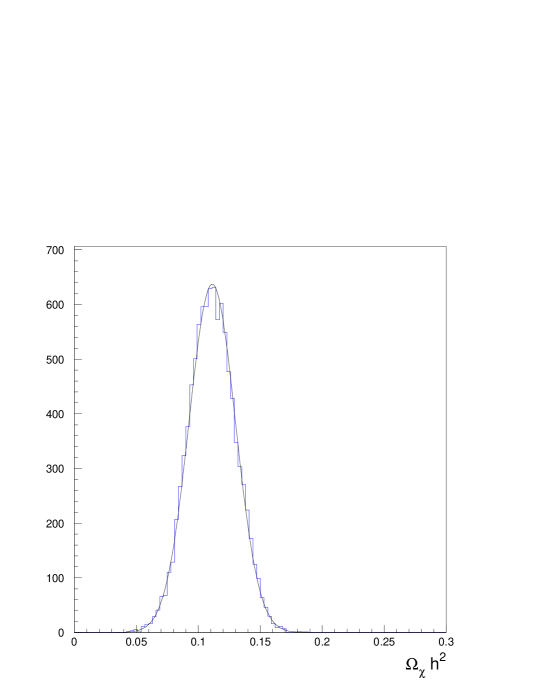
Figure 13: The estimated accuracy with which $\Omega_{\chi}h^{2}$ could be predicted on the basis of LHC data for the updated benchmark point B, using the projected experimental errors reported in  [40], a fit to ISASUGRA 7.67 parameters and the Micromegas code. We find similar results using SSARD.

As seen in Fig. 13, the calculated relic density has a well-behaved distribution that is well fit by a Gaussian with

$$\Omega_{\chi}h^{2}=0.111\pm 0.018$$ (15)

We have made a similar analysis using SSARD, finding an identical central value of $\Omega_{\chi}h^{2}$ and errors ${}^{+0.014}_{-0.020}$, ${}^{+0.001}_{-0.000}$ and ${}^{+0.010}_{-0.017}$ associated with $m_{0}$, $m_{1/2}$ and $\tan\beta$, respectively. We conclude that collider measurements should, in principle enable the expected value of $\Omega_{\chi}h^{2}$ to be calculated with interesting accuracy. Measurements at linear $e^{+}e^{-}$ colliders would increase the accuracy in (15) and also enable $\Omega_{\chi}h^{2}$ to be calculated for other benchmarks where data from the LHC alone might be insufficient.

The LHC and linear $e^{+}e^{-}$ collider measurements would also provide crucial input for predicting the cross sections expected in direct dark matter searches or the LSP annihilation rate in the Sun. For this, it would in general be important to measure the higgsino and gaugino components of the LSP, which may be possible at the LHC in some regions of the parameter space by measuring the decay modes of the heavier gauginos or by comparing the rates of $\chi_{2}\to\ell\ell\chi$ via a (virtual) slepton and $\chi_{2}\to\chi h$.

Dark matter physics is another example of the complementarity of LHC and linear $e^{+}e^{-}$ colliders for exploring new physics in the TeV energy range. Very possibly, Nature does not choose the CMSSM, and it is desirable to formulate benchmarks for other possibilities [8]. However, the CMSSM remains one of the prime options for physics beyond the Standard Model that might be accessible to the next generation of colliders. We hope that this paper contributes to a better understanding of what they might achieve, given the present constraints on supersymmetry from laboratory experiments and cosmology, as updated here using information from WMAP.

Acknowledgments
The work of K.A.O. was supported partly by DOE grant DE–FG02–94ER–40823. We thank G. Belanger, F. Boudjema and A. Pukhov for useful discussions about Micromegas.

References

- [1] L. Maiani, Proceedings of the 1979 Gif-sur-Yvette Summer School On Particle Physics, 1; G. ’t Hooft, in Recent Developments in Gauge Theories, Proceedings of the Nato Advanced Study Institute, Cargese, 1979, eds. G. ’t Hooft et al., (Plenum Press, NY, 1980); E. Witten, Phys. Lett. B 105, 267 (1981).
- [2] I. Hinchliffe, F. E. Paige, M. D. Shapiro, J. Soderqvist and W. Yao, Phys. Rev. D55 (1997) 5520; S. Abdullin et al. [CMS Collaboration], hep-ph/9806366; S. Abdullin and F. Charles, Nucl. Phys. B547 (1999) 60; TESLA Technical Design Report, DESY-01-011, Part III, Physics at an Linear Collider (March 2001).
- [3] M. Battaglia et al., Eur. Phys. J. C 22, 535 (2001) [arXiv:hep-ph/0106204].
-
[4]
Joint LEP 2 Supersymmetry Working Group,
Combined LEP Chargino Results, up to 208 GeV,
http://lepsusy.web.cern.ch/lepsusy/www/inos_moriond01/ charginos_pub.html; Combined LEP Selectron/Smuon/Stau Results, 183-208 GeV,
http://lepsusy.web.cern.ch/lepsusy/www/sleptons_summer02/ slep_2002.html. - [5] LEP Higgs Working Group for Higgs boson searches, OPAL Collaboration, ALEPH Collaboration, DELPHI Collaboration and L3 Collaboration, Search for the Standard Model Higgs Boson at LEP, CERN-EP/2003-011, arXiv:hep-ex/0306033.
- [6] M. S. Alam et al., [CLEO Collaboration], Phys. Rev. Lett. 74, 2885 (1995), as updated in S. Ahmed et al., CLEO CONF 99-10; BELLE Collaboration, BELLE-CONF-0003, contribution to the 30th International conference on High-Energy Physics, Osaka, 2000. See also K. Abe et al., [Belle Collaboration], arXiv:hep-ex/0107065; L. Lista [BaBar Collaboration], arXiv:hep-ex/0110010; C. Degrassi, P. Gambino and G. F. Giudice, JHEP 0012, 009 (2000) [arXiv:hep-ph/0009337]; M. Carena, D. Garcia, U. Nierste and C. E. Wagner, Phys. Lett. B 499, 141 (2001) [arXiv:hep-ph/0010003]; P. Gambino and M. Misiak, Nucl. Phys. B 611, 338 (2001); D. A. Demir and K. A. Olive, Phys. Rev. D 65, 034007 (2002) [arXiv:hep-ph/0107329]; T. Hurth, arXiv:hep-ph/0212304.
- [7] H. N. Brown et al. [Muon g-2 Collaboration], Phys. Rev. Lett. 86, 2227 (2001) [arXiv:hep-ex/0102017]; G. W. Bennett et al. [Muon g-2 Collaboration], Phys. Rev. Lett. 89, 101804 (2002) [Erratum-ibid. 89, 1219903 (2002)] [arXiv:hep-ex/0208001]; M. Davier, S. Eidelman, A. Hocker and Z. Zhang, Eur. Phys. J. C 27, 497 (2003) [arXiv:hep-ph/0208177]; see also K. Hagiwara, A. D. Martin, D. Nomura and T. Teubner, arXiv:hep-ph/0209187; F. Jegerlehner, unpublished, as reported in M. Krawczyk, arXiv:hep-ph/0208076.
- [8] B. C. Allanach et al., Proc. of the APS/DPF/DPB Summer Study on the Future of Particle Physics (Snowmass 2001) ed. N. Graf, Eur. Phys. J. C 25, 113 (2002) [eConf C010630, P125 (2001)] [arXiv:hep-ph/0202233].
- [9] M. Carena, S. Heinemeyer, C. E. Wagner and G. Weiglein, arXiv:hep-ph/9912223, Eur. Phys. J. C 26, 601 (2003) [arXiv:hep-ph/0202167].
- [10] G. L. Kane, J. Lykken, S. Mrenna, B. D. Nelson, L. T. Wang and T. T. Wang, Phys. Rev. D 67, 045008 (2003) [arXiv:hep-ph/0209061].
- [11] H. Baer, T. Krupovnickas and X. Tata, arXive:hep-ph/0305325.
- [12] C. L. Bennett et al., arXiv:astro-ph/0302207; D. N. Spergel et al., arXiv:astro-ph/0302209; H. V. Peiris et al., arXiv:astro-ph/0302225.
- [13] J. R. Ellis, J. S. Hagelin, D. V. Nanopoulos, K. A. Olive and M. Srednicki, Nucl. Phys. B 238, 453 (1984); see also H. Goldberg, Phys. Rev. Lett. 50, 1419 (1983).
- [14] See, for example: J. R. Ellis, T. Falk, G. Ganis, K. A. Olive and M. Srednicki, Phys. Lett. B510, 236 (2001) [arXiv:hep-ph/0102098]; L. Roszkowski, R. Ruiz de Austri and T. Nihei, JHEP 0108, 204 (2001) [arXiv:hep-ph/0106334]; A. Djouadi, M. Drees and J. L. Kneur, JHEP 0108, 055 (2001) [arXiv:hep-ph/0107316]; U. Chattopadhyay, A. Corsetti and P. Nath, Phys. Rev. D 66, 035003 (2002) [arXiv:hep-ph/0201001]; H. Baer, C. Balazs and A. Belyaev, JHEP 0203, 042 (2002) [arXiv:hep-ph/0202076]; R. Arnowitt and B. Dutta, arXiv:hep-ph/0211417; T. Kamon, R. Arnowitt, B. Dutta and V. Khotilovich, arXiv:hep-ph/0302249; H. Baer, C. Balazs, A. Belyaev, T. Krupovnickas and X. Tata, arXiv:hep-ph/0304303.
- [15] J. Ellis, K. A. Olive, Y. Santoso and V. C. Spanos, arXiv:hep-ph/0303043.
- [16] H. Baer and C. Balazs, arXiv:hep-ph/0303114; A. B. Lahanas and D. V. Nanopoulos, arXiv:hep-ph/0303130; U. Chattopadhyay, A. Corsetti and P. Nath, arXiv:hep-ph/0303201.
- [17] A. B. Lahanas, D. V. Nanopoulos and V. C. Spanos, Phys. Rev. D 62 (2000) 023515 [arXiv:hep-ph/9909497]; Mod. Phys. Lett. A 16 (2001) 1229 [arXiv:hep-ph/0009065]; Phys. Lett. B518 (2001) 94 [arXiv:hep-ph/0107151]; V. Barger and C. Kao, Phys. Lett. B518 (2001) 117 [arXiv:hep-ph/0106189]; R. Arnowitt and B. Dutta, arXiv:hep-ph/0211417.
- [18] Information about this code is available from K. A. Olive: it contains important contributions from T. Falk, G. Ganis, J. McDonald, K. A. Olive and M. Srednicki.
- [19] S. Heinemeyer, W. Hollik and G. Weiglein, Comput. Phys. Commun. 124, 76 (2000) [hep-ph/9812320] and Eur. Phys. J. C 9 (1999) 343 [arXiv:hep-ph/9812472].
- [20] We use mainly the 7.67 version of ISASUGRA, whose basic documentation is found in H. Baer, F. E. Paige, S. D. Protopopescu and X. Tata, ISAJET 7.48: A Monte Carlo event generator for , , and reactions, hep-ph/0001086. The latest update is available from http://paige.home.cern.ch/paige/.
- [21] S. Matsumoto et al. [JLC Group], JLC-1, KEK Report 92-16 (1992); J. Bagger et al. [American Linear Collider Working Group], The Case for a 500-GeV Linear Collider, SLAC-PUB-8495, BNL-67545, FERMILAB-PUB-00-152, LBNL-46299, UCRL-ID-139524, LBL-46299, Jul 2000, arXiv:hep-ex/0007022; T. Abe et al. [American Linear Collider Working Group Collaboration], Linear Collider Physics Resource Book for Snowmass 2001, SLAC-570, arXiv:hep-ex/0106055, hep-ex/0106056, hep-ex/0106057 and hep-ex/0106058; TESLA Technical Design Report, DESY-01-011, Part III, Physics at an Linear Collider (March 2001).
- [22] R. W. Assmann et al. [CLIC Study Team], A 3-TeV Linear Collider Based on CLIC Technology, ed. G. Guignard, CERN 2000-08; for more information about this project, see: http://ps-div.web.cern.ch/ps-div/CLIC/Welcome.html.
- [23] CLIC Physics Study Group, http://clicphysics.web.cern.ch/CLICphysics/ and Yellow Report in preparation.
- [24] M. Drees, Y. G. Kim, M. M. Nojiri, D. Toya, K. Hasuko and T. Kobayashi, Phys. Rev. D 63, 035008 (2001) [arXiv:hep-ph/0007202].
- [25] J. Ellis, T. Falk and K. A. Olive, Phys. Lett. B 444, 367 (1998) [arXiv:hep-ph/9810360]; J. Ellis, T. Falk, K. A. Olive and M. Srednicki, Astropart. Phys. 13, 181 (2000) [arXiv:hep-ph/9905481]; M. E. Gómez, G. Lazarides and C. Pallis, Phys. Rev. D 61, 123512 (2000) [arXiv:hep-ph/9907261], Phys. Lett. B 487, 313 (2000) [arXiv:hep-ph/0004028] and Nucl. Phys. B B638, 165 (2002) [arXiv:hep-ph/0203131]; R. Arnowitt, B. Dutta and Y. Santoso, Nucl. Phys. B 606, 59 (2001) [arXiv:hep-ph/0102181]; T. Nihei, L. Roszkowski and R. Ruiz de Austri, JHEP 0207, 024 (2002) [arXiv:hep-ph/0206266].
- [26] M. Drees and M. M. Nojiri, Phys. Rev. D 47, 376 (1993) [arXiv:hep-ph/9207234]; H. Baer and M. Brhlik, Phys. Rev. D 53, 597 (1996) [arXiv:hep-ph/9508321] and Phys. Rev. D 57, 567 (1998) [arXiv:hep-ph/9706509]; H. Baer, M. Brhlik, M. A. Diaz, J. Ferrandis, P. Mercadante, P. Quintana and X. Tata, Phys. Rev. D 63, 015007 (2001) [arXiv:hep-ph/0005027]; A. B. Lahanas, D. V. Nanopoulos and V. C. Spanos, Mod. Phys. Lett. A 16, 1229 (2001) [arXiv:hep-ph/0009065]; J. R. Ellis, T. Falk, G. Ganis, K. A. Olive and M. Srednicki in [14]; A. B. Lahanas and V. C. Spanos, Eur. Phys. J. C 23, 185 (2002) [arXiv:hep-ph/0106345].
- [27] J. L. Feng, K. T. Matchev and T. Moroi, Phys. Rev. Lett. 84 (2000) 2322; J. L. Feng, K. T. Matchev and T. Moroi, Phys. Rev. D61 (2000) 075005; J. L. Feng, K. T. Matchev and F. Wilczek, Phys. Lett. B482 (2000) 388.
- [28] A. Djouadi, J.-L. Kneur and G. Moultaka, SuSpect: a Fortran Code for the Supersymmetric and Higgs Particle Spectrum in the MSSM, arXiv:hep-ph/0211331. The latest version is available from http://www.lpm.univ-montp2.fr:7082/~kneur/.
-
[29]
B. C. Allanach, S. Kraml and W. Porod,
JHEP 0303, 016 (2003)
[arXiv:hep-ph/0302102]; see also the web pages
http://cern.ch/kraml/comparison/compare.html for comparisons between different codes and http://wwwth.cern.ch/susycom/compare_vrsn.html for comparisons between different versions of ISASUGRA. -
[30]
The RunII D0 top group, see
http://www-d0.fnal.gov/Run2Physics/top/conf.html. - [31] D. Pierce and A. Papadopoulos, Phys. Rev. D50, 565 (1994) [hep-ph/9312248] and Nucl. Phys. B430, 278 (1994) [hep-ph/9403240]; W. de Boer, R. Ehret and D. I. Kazakov, Z. Phys. C 67, 647 (1995) [arXiv:hep-ph/9405342]; D. M. Pierce, J. A. Bagger, K. Matchev and R. Zhang, Nucl. Phys. B491, 3 (1997) [hep-ph/9606211].
- [32] J. R. Ellis, K. Enqvist, D. V. Nanopoulos and F. Zwirner, Mod. Phys. Lett. A 1, 57 (1986); R. Barbieri and G. F. Giudice, Nucl. Phys. B 306, 63 (1988); J. R. Ellis and K. A. Olive, Phys. Lett. B 514, 114 (2001) [arXiv:hep-ph/0105004]; J. R. Ellis, K. A. Olive and Y. Santoso, New J. Phys. 4, 32 (2002) [arXiv:hep-ph/0202110].
- [33] G. Belanger, F. Boudjema, A. Pukhov and A. Semenov, arXiv:hep-ph/0112278.
- [34] T. Sjostrand, L. Lonnblad and S. Mrenna, arXiv:hep-ph/0108264.
- [35] ATLAS Collaboration, ATLAS detector and physics performance Technical Design Report, CERN/LHCC 99-14/15 (1999); CMS Collaboration, Technical Proposal, CERN/LHCC 94-38 (1994).
- [36] See [35], and the second and third papers in [2].
- [37] M. Kazana, G. Wrochna and P. Zalewski, CMS Conference Report 1999-019, contributed to the European Physical Society Conference on High-Energy Physics, Tampere, 1999.
- [38] M. Pohl and H. J. Schreiber, arXiv:hep-ex/0206009.
- [39] M. Battaglia and M. Gruwe, arXiv:hep-ph/0212140.
- [40] G. Polesello, private communication.