Bicocca-FT-03-12

CERN–TH/2003-117

hep-ph/0306211

Soft-gluon resummation for Higgs boson production
at hadron colliders

Stefano Catani^(a), Daniel de Florian^(b), Massimiliano Grazzini^(c) and Paolo Nason^(d)

^(a)INFN, Sezione di Firenze, I-50019 Sesto Fiorentino, Florence, Italy

^(b)Departamento de Física, FCEYN, Universidad de Buenos Aires, (1428) Pabellón 1

Ciudad Universitaria, Capital Federal, Argentina

^(c)Theory Division, CERN, CH-1211 Geneva 23, Switzerland

^(d)INFN, Sezione di Milano, I-20136 Milan, Italy

Abstract

We consider QCD corrections to Higgs boson production through gluon–gluon fusion in hadron collisions. We compute the cross section, performing the all-order resummation of multiple soft-gluon emission at next-to-next-to-leading logarithmic level. Known fixed-order results (up to next-to-next-to-leading order) are consistently included in our calculation. We give phenomenological predictions for Higgs boson production at the Tevatron and at the LHC. We estimate the residual theoretical uncertainty from perturbative QCD contributions. We also quantify the differences obtained by using the presently available sets of parton distributions.

CERN–TH/2003-117

June 2003

1 Introduction

Higgs boson production is nowadays a topic of central importance in hadron collider physics [1, 2]. The Tevatron will be actively searching for a Higgs boson signal in the near future. The discovery of the Higgs boson is also a primary physics goal of the LHC.

The main Higgs production mechanism at hadron colliders is the gluon fusion process [3], an essentially strong-interaction process, that has attracted a large amount of theoretical work in recent years. Indeed, limits on the Higgs mass will rely upon QCD calculations of the cross sections. Conversely, if a Higgs boson is discovered, discrepancies of its measured cross section from QCD calculations may signal deviations of the Yukawa couplings from the Standard Model (SM) predictions. It is thus important to provide an accurate calculation of the Higgs production cross section, together with a reliable estimate of the associated theoretical error.

The QCD computation of the gluon fusion production cross section was carried out at next-to-leading order (NLO) in Refs. [4, 5] in the heavy-top limit, and in Ref. [6] with the full dependence on the top-quark mass. Perturbative corrections at the NLO level were found to be quite large (of the order of 100%), thus casting doubts upon the reliability of the perturbative calculation.

Next-to-next-to-leading order (NNLO) corrections have been computed in the heavy-top limit. The virtual contributions were evaluated in Ref. [7]. The soft contributions were computed in Refs. [8, 9]. The remaining hard real contributions were included in Ref. [10], with a semi-numerical approach. More recently, fully analytical results for the real contributions have been obtained [11, 12, 13].

Numerically, it is found that NNLO corrections are moderate in size. There is thus good hope that the NNLO calculation gives a reasonable estimate of the cross section. Nevertheless, a better understanding of the pattern of radiative corrections would prove useful both to assess the reliability of the available calculations and to include higher-order corrections.

In the present work, we include the dominant effect of the uncalculated higher-order terms, by exploiting the resummation of soft-gluon emission. The possibility of performing such an improvement relies upon the observation that an accurate use of the soft-gluon approximation provides the bulk of the NLO term and a reliable estimate of the NNLO effects [8]. Now that the NNLO corrections are fully known, and confirm that observation, it makes sense to add the higher-order terms that can be obtained in the soft-gluon approximation, in order to give a more precise prediction. Since the soft approximation proves reliable for the NLO and NNLO contributions, we make the reasonable assumption that it maintains the same reliability for higher-order terms.

The paper is organized as follows. In Sect. 2 we give our notation for the QCD cross section and the fixed-order radiative corrections. In Sect. 3 we present the formalism of soft-gluon resummation to all logarithmic orders, and derive the explicit resummation formulae up to the next-to-next-to-leading logarithmic (NNLL) level.

The resummation formalism correctly predicts the structure and the coefficients of the singular terms in the exact NLO and NNLO calculations. The quantitative reliability of the soft-gluon approximation can be tested by comparing the truncation of the resummation formalism at the NLO and NNLO levels with the exact result. This comparison is performed in Sect. 4. Several variants of the soft-gluon approximation are considered there, in order to justify the validity of our approach. Furthermore, in Sect. 4.2, the order of magnitude of the soft-gluon effects is studied, by simply considering the value of the short-distance partonic cross section in $N$-moment space.

In Sect. 5, full numerical predictions for the Higgs production cross section, including soft-gluon resummation at NNLL accuracy and the exact NLO and NNLO contributions, are given, both at the Tevatron and at the LHC. We also perform a study of the remaining theoretical uncertainty. Incidentally, we note that the calculation presented here is the first calculation of a QCD cross section at such nominal theoretical accuracy, namely NNLO+NNLL accuracy.

Finally, in Sect. 6 we give our conclusions.

In Appendix A we derive a simple prescription to evaluate the large-$N$ Mellin moments of the soft-gluon contributions at an arbitrary logarithmic accuracy. The method is a generalization of the prescription $z^{N-1}-1\rightarrow-\theta(1-z-N_{0}/N)$. In Appendix B, we present a formal proof of the equivalence of two different formulations of the $N$-space resummation formulae. This equivalence clarifies the distinction between the all-order logarithmic terms in the soft-gluon resummation formalism and the large-order perturbative behaviour due to infrared renormalons. In Appendix C we show how to compute the logarithmic functions that control soft-gluon resummation. In Appendix D we check the numerical convergence of the fixed-order soft-gluon expansion, and in Appendix E we provide the soft-gluon approximation of the N³LO contribution to the partonic cross section.

Preliminary results of this work have been presented in Ref. [14].

2 Notation and QCD cross section at fixed orders

We consider the collision of two hadrons $h_{1}$ and $h_{2}$ with centre-of-mass energy ${\sqrt{s}}$. The inclusive cross section for the production of the SM Higgs boson can be written as

$$\sigma(s,M_{H}^{2})= \sum_{a,b}\int_{0}^{1}dx_{1}\;dx_{2}\;f_{a/h_{1}}(x_{1},\mu_{F}^{2})\;f_{b/h_{2}}(x_{2},\mu_{F}^{2})\int_{0}^{1}dz\;\delta\!\left(z-\frac{\tau_{H}}{x_{1}x_{2}}\right)$$

$$\cdot\sigma^{(0)}\,z\;G_{ab}(z;\alpha_{\mathrm{S}}(\mu_{R}^{2}),M_{H}^{2}/\mu_{R}^{2};M_{H}^{2}/\mu_{F}^{2})\;,$$ (1)

where $M_{H}$ is the Higgs boson mass, $\tau_{H}=M_{H}^{2}/s$, and $\mu_{F}$ and $\mu_{R}$ are factorization and renormalization scales, respectively. The parton densities of the colliding hadrons are denoted by $f_{a/h}(x,\mu_{F}^{2})$ and the subscript $a$ labels the type of massless partons ($a=g,q_{f},{\bar{q}}_{f}$, with $N_{f}$ different flavours of light quarks). We use parton densities as defined in the ${\overline{\rm MS}}$ factorization scheme.

From Eq. (2) the cross section ${\hat{\sigma}}_{ab}$ for the partonic subprocess $ab\rightarrow H+X$ at the centre-of-mass energy ${\hat{s}}=x_{1}x_{2}s=M_{H}^{2}/z$ is

$${\hat{\sigma}}_{ab}({\hat{s}},M_{H}^{2})=\frac{1}{\hat{s}}\;\sigma^{(0)}M_{H}^{2}\;G_{ab}(z)=\sigma^{(0)}\;z\;\;G_{ab}(z)\;,$$ (2)

where the term $1/{\hat{s}}$ corresponds to the flux factor and leads to an overall $z$ factor. The Born-level cross section $\sigma^{(0)}$ and the hard coefficient function $G_{ab}$ arise from the phase-space integral of the matrix elements squared.

The incoming partons $a,b$ couple to the Higgs boson through heavy-quark loops and, therefore, $\sigma^{(0)}$ and $G_{ab}$ also depend on the masses $M_{Q}$ of the heavy quarks. The Born-level contribution $\sigma^{(0)}$ is [3]

$$\sigma^{(0)}=\frac{G_{F}}{288\pi\sqrt{2}}\;\left|\sum_{Q}A_{Q}\!\left(\frac{4M_{Q}^{2}}{M_{H}^{2}}\right)\right|^{2}\;\;,$$ (3)

where $G_{F}=1.16639\times 10^{-5}$ GeV^-2 is the Fermi constant, and the amplitude $A_{Q}$ is given by

$$A_{Q}(x) =\frac{3}{2}x\Big{[}1+(1-x)f(x)\Big{]}\;,$$

$$f(x) =\left\{\begin{array}[]{ll}\displaystyle\arcsin^{2}\frac{1}{\sqrt{x}}\;,&x\geq 1\\ \displaystyle-\frac{1}{4}\left[\ln\frac{1+\sqrt{1-x}}{1-\sqrt{1-x}}-i\pi\right]^{2}\;,&x<1\end{array}\right.\;.$$ (6)

In the following, $M_{Q}=M_{t}$ or $M_{b}$ denotes the on-shell pole mass of the top quark or bottom quark.

The coefficient function $G_{ab}$ in Eq. (2) is computable in QCD perturbation theory according to the expansion

$$G_{ab}(z;\alpha_{\mathrm{S}}(\mu_{R}^{2}),M_{H}^{2}/\mu_{R}^{2};M_{H}^{2}/\mu_{F}^{2})=\alpha_{\mathrm{S}}^{2}(\mu_{R}^{2})\sum_{n=0}^{+\infty}\left(\frac{\alpha_{\mathrm{S}}(\mu_{R}^{2})}{\pi}\right)^{n}\;G_{ab}^{(n)}(z;M_{H}^{2}/\mu_{R}^{2};M_{H}^{2}/\mu_{F}^{2})$$ (7)

$$=\alpha_{\mathrm{S}}^{2}(\mu_{R}^{2})G_{ab}^{(0)}(z)+\frac{\alpha_{\mathrm{S}}^{3}(\mu_{R}^{2})}{\pi}\;G_{ab}^{(1)}\left(z;\frac{M_{H}^{2}}{\mu_{R}^{2}};\frac{M_{H}^{2}}{\mu_{F}^{2}}\right)+\frac{\alpha_{\mathrm{S}}^{4}(\mu_{R}^{2})}{\pi^{2}}\;G_{ab}^{(2)}\left(z;\frac{M_{H}^{2}}{\mu_{R}^{2}};\frac{M_{H}^{2}}{\mu_{F}^{2}}\right)+{\cal O}(\alpha_{\mathrm{S}}^{5})\;,$$ (8)

where the (scale-independent) LO contribution is

$$G_{ab}^{(0)}(z)=\delta_{ag}\;\delta_{bg}\;\delta(1-z)\;.$$ (9)

The terms $G_{ab}^{(1)}$ and $G_{ab}^{(2)}$ give the NLO and NNLO contributions, respectively.

The NLO coefficients $G_{ab}^{(1)}$ are known. Their calculation with the exact dependence on $M_{t}$ (and $M_{b}$) was performed in Ref. [6], where it was also observed that the NLO Higgs boson cross section is well approximated by considering its limit $M_{t}\gg M_{H}$ [4, 5]. Therefore, throughout the paper we work in the framework of the large-$M_{t}$ approximation: we consider the case of a single heavy quark, the top quark, and $N_{f}=5$ light-quark flavours, and we neglect all the contributions to $G_{ab}^{(n)}$ that vanish when $M_{H}/M_{t}\rightarrow 0$. However, unless otherwise stated, we include in $\sigma^{(0)}$ the full dependence on $M_{t}$ and $M_{b}$. At NLO this approximation [6, 15] turns out to be very good when $M_{H}\leq 2M_{t}$, and it is still accurate to better than $10\%$ when $M_{H}\raisebox{-1.72218pt}{\hbox to0.0pt{$\,\sim\,$\hss}}\raisebox{1.72218pt}{$\,<\,$}1$ TeV.

The use of the large-$M_{t}$ expansion considerably simplifies the calculation of the QCD radiative corrections, since one can exploit the effective-lagrangian approach [17, 18, 15] to embody the heavy-quark loop in an effective point-like vertex. The virtual [7] and soft [19, 20, 21, 22] contributions (i.e. the contributions that are singular when $z\rightarrow 1$) to the NNLO coefficients $G_{ab}^{(2)}(z)$ were independently computed in Refs. [8] and [9]. The hard contributions were considered in Ref. [10], by expanding $G_{ab}^{(2)}(z)$ in powers of $(1-z)$ and evaluating the coefficients of the expansion explicitly up to order $(1-z)^{16}$. An independent NNLO calculation, which includes all the hard contributions in closed analytic form, was carried out in Ref. [11]. This result has recently been confirmed [13] by using a different method of calculation. In the high-energy limit, the results of Refs. [11, 13] agree with the calculation of Ref. [23], based on $k_{\perp}$-factorization [24].

The NLO coefficient functions $G_{ab}^{(1)}$ in the large-$M_{t}$ limit (i.e. neglecting corrections that vanish when $M_{H}/M_{t}\rightarrow 0$) are [4, 5]

$$G_{gg}^{(1)}(z;M_{H}^{2}/\mu_{R}^{2}; M_{H}^{2}/\mu_{F}^{2})=\delta(1-z)\left(\frac{11}{2}+6\zeta(2)+\frac{33-2N_{f}}{6}\ln\frac{\mu_{R}^{2}}{\mu_{F}^{2}}\right)+12\,{\cal D}_{1}(z)$$

$$+6\,{\cal D}_{0}(z)\,\ln\frac{M_{H}^{2}}{\mu_{F}^{2}}\,+P_{gg}^{{\rm reg}}(z)\,\ln\frac{(1-z)^{2}M_{H}^{2}}{z\mu_{F}^{2}}-6\frac{\ln z}{1-z}-\frac{11}{2}\frac{(1-z)^{3}}{z}\;,$$ (10)

$$G_{gq}^{(1)}(z;M_{H}^{2}/\mu_{R}^{2};M_{H}^{2}/\mu^{2}_{F})=\frac{1}{2}P_{gq}(z)\ln\frac{(1-z)^{2}M_{H}^{2}}{z\mu^{2}_{F}}+\frac{2}{3}\,z-\frac{(1-z)^{2}}{z}\;,$$ (11)

$$G_{q{\bar{q}}}^{(1)}(z;M_{H}^{2}/\mu_{R}^{2};M_{H}^{2}/\mu_{F}^{2})=\frac{32}{27}\,\frac{(1-z)^{3}}{z}\;,\quad G_{qq}^{(1)}(z;M_{H}^{2}/\mu_{R}^{2};M_{H}^{2}/\mu_{F}^{2})=0\;,$$ (12)

where $\zeta(n)$ is the Riemann zeta-function ($\zeta(2)=\pi^{2}/6=1.645\dots$, $\zeta(3)=1.202\dots$), and we have defined

$${\cal D}_{i}(z)\equiv\left[\frac{\ln^{i}(1-z)}{1-z}\right]_{+}\,\,.$$ (13)

The kernels $P_{ab}(z)$ are the LO Altarelli–Parisi splitting functions for real emission,

$$P_{gg}(z)=6\left[\frac{1}{1-z}+\frac{1}{z}-2+z(1-z)\right]\;,~{}~{}~{}~{}~{}P_{gq}(z)=\frac{4}{3}\,\frac{1+(1-z)^{2}}{z}\;,$$ (14)

and $P_{gg}^{{\rm reg}}(z)$ is the regular (when $z\rightarrow 1$) part of $P_{gg}(z)$:

$$P_{gg}^{{\rm reg}}(z)=P_{gg}(z)-\frac{6}{1-z}\;.$$ (15)

The analytic formulae for the NNLO coefficient functions $G_{ab}^{(2)}$ are given in Refs. [11, 13] ($\eta_{ab}^{(2)}(z)=zG_{ab}^{(2)}(z)$, according to the notation of Ref. [11]).

For the purpose of the discussion in the following sections, we note that we can identify three kinds of contributions in Eqs. (2)–(12) and in the analytic formulae for $G_{ab}^{(2)}$:

• Soft and virtual corrections, which involve only the $gg$ channel and give rise to the ${\cal D}_{i}$ and $\delta(1-z)$ terms (see Eq. (2)). These are the most singular terms when $z\rightarrow 1$.

• Purely collinear logarithmic contributions, which are controlled by the regular part of the Altarelli–Parisi splitting kernels (see Eqs. (2), (11)). The argument of the collinear logarithm corresponds to the maximum value $(q^{2}_{T\,{\rm max}}\sim(1-z)^{2}M_{H}^{2}/z)$ of the transverse momentum $q_{T}$ of the Higgs boson. These contributions give the next-to-dominant singular terms when $z\rightarrow 1$.

• Hard contributions, which are present in all partonic channels and lead to finite corrections in the limit $z\rightarrow 1$ .

In this work we are mainly interested in studying the effect of soft-gluon contributions to all perturbative orders. Soft-gluon resummation has to be carried out in the Mellin (or $N$-moment) space [25, 26]. We thus introduce our notation in the $N$-space.

We consider the Mellin transform $\sigma_{N}(M_{H}^{2})$ of the hadronic cross section $\sigma(s,M_{H}^{2})$. The $N$-moments with respect to $\tau_{H}=M_{H}^{2}/s$ at fixed $M_{H}$ are thus defined as follows:

$$\sigma_{N}(M_{H}^{2})\equiv\int_{0}^{1}\;d\tau_{H}\;\tau_{H}^{N-1}\;\sigma(s,M_{H}^{2})\;\;.$$ (16)

In $N$-moment space, Eq. (2) takes a simple factorized form

$$\sigma_{N-1}(M_{H}^{2})=\sigma^{(0)}\;\sum_{a,b}\;f_{a/h_{1},\,N}(\mu_{F}^{2})\;f_{b/h_{2}\,N}(\mu_{F}^{2})\;{G}_{ab,\,N}(\alpha_{\mathrm{S}}(\mu_{R}^{2}),M_{H}^{2}/\mu_{R}^{2};M_{H}^{2}/\mu_{F}^{2})\;,$$ (17)

where we have introduced the customary $N$-moments of the parton distributions ($f_{a/h,\,N}$) and of the hard coefficient function (${G}_{ab,\,N}$):

$$f_{a/h,\,N}(\mu_{F}^{2}) =\int_{0}^{1}\;dx\;x^{N-1}\;f_{a/h}(x,\mu_{F}^{2})\;,$$ (18)

$$G_{ab,\,N} =\int_{0}^{1}dz\;z^{N-1}\;G_{ab}(z)\;\;.$$ (19)

Once these $N$-moments are known, the physical cross section in $x$-space can be obtained by Mellin inversion:

$$\sigma(s,M_{H}^{2})=\sigma^{(0)}\;\sum_{a,b} \;\int_{C_{MP}-i\infty}^{C_{MP}+i\infty}\;\frac{dN}{2\pi i}\;\left(\frac{M_{H}^{2}}{s}\right)^{-N+1}\;f_{a/h_{1},\,N}(\mu_{F}^{2})\;f_{b/h_{2}\,N}(\mu_{F}^{2})$$

$$\times\;{G}_{ab,\,N}(\alpha_{\mathrm{S}}(\mu_{R}^{2}),M_{H}^{2}/\mu_{R}^{2};M_{H}^{2}/\mu_{F}^{2})\;,$$ (20)

where the constant $C_{MP}$ that defines the integration contour in the $N$-plane is on the right of all the possible singularities of the $N$-moments.

Note that the evaluation of $G_{ab}(z)$ in the limit $z\rightarrow 1$ corresponds to the evaluation of its $N$-moments $G_{ab,N}$ in the limit $N\rightarrow\infty$. In particular, the soft, virtual and collinear contributions to $G_{ab}^{(n)}(z)$ lead to $\ln N$-enhanced contributions in $N$-space according to the following correspondence (see Appendix A):

$$\int_{0}^{1}\;dz\;z^{N-1}\;{\cal D}_{k}(z) =\frac{(-1)^{k+1}}{k+1}\ln^{k+1}N+{\cal O}(\ln^{k}N)\;\;,$$ (21)

$$\int_{0}^{1}\;dz\;z^{N-1}\;\delta(1-z) =1\;\;,$$ (22)

$$\int_{0}^{1}\;dz\;z^{N-1}\;\ln^{k}(1-z) =\frac{(-1)^{k}}{N}\ln^{k}N+{\cal O}\left(\frac{1}{N}\ln^{k-1}N\right)\;\;.$$ (23)

3 Soft-gluon resummation

3.1 Summation to all logarithmic orders

In this section we consider the all-order perturbative summation of enhanced threshold (soft and virtual) contributions to the partonic cross section for Higgs boson production. The threshold region $z\rightarrow 1$ corresponds to the limit $N\rightarrow\infty$ in $N$-moment space. We are thus interested in evaluating the hard coefficient function $G_{ab,\,N}$, by keeping all the terms that are not vanishing when $N\rightarrow\infty$. To this purpose, we first note that in this limit only the $gg$ partonic channel is not suppressed. In other words, we have:

$$G_{ab,\,N}(\alpha_{\mathrm{S}}(\mu_{R}^{2}),M_{H}^{2}/\mu_{R}^{2};M_{H}^{2}/\mu_{F}^{2})={\cal O}(1/N)\;\;\quad(ab\neq gg)\;\;,$$ (24)

where the notation ${\cal O}(1/N)$ means that the right-hand side vanishes at least as a single power of $1/N$ (modulo $\ln N$ corrections) when $N\rightarrow\infty$. When the partonic channel is $ab\neq q{\bar{q}}$, Eq. (24) simply follows from power counting: the final state $X$ in the partonic subprocess $ab\rightarrow{H+X}$ contains at least a fermion, and the corresponding cross section thus vanishes in the soft limit. When $ab=q{\bar{q}}$, the threshold limit selects the exclusive subprocess $q{\bar{q}}\rightarrow H$ that vanishes since the gluon-mediated production of a spin 0 particle through $q{\bar{q}}$ annihilation is forbidden in the massless quark case. As a matter of fact, gluonic interactions conserve helicity, so that the total spin projection along the incoming $q\bar{q}$ direction is $\pm 1$, which is incompatible with the production of a spin 0 state.

Observe that the large-$N$ behaviour of the hadronic cross section $\sigma_{N}(M_{H}^{2})$ also depends upon the large-$N$ behaviour of the parton densities, according to Eq. (17). Thus, the ${\cal O}(1/N)$ relative suppression of the partonic cross section in the $qg$ channel relative to the $gg$ channel may be compensated by the enhancement of the quark with respect to the gluon density. Under the typical assumption that the gluon density is softer than the (valence) quark density at large $x$, it is possible to show (see Sect. 2.4 in Ref. [27]) that the two parton channels contribute with the same power behaviour in $N$ to the total hadronic cross section. In the present work, however, we are not considering the large-$N$ limit of the hadronic cross section $\sigma_{N}(M_{H}^{2})$ for Higgs boson production. We are rather using the soft-gluon approximation to find a good approximation of the full partonic cross section, to be convoluted with the parton densities and used in kinematical regimes that are far from the hadronic large-$N$ limit. In this context, Eq. (24) implies that the $gg$ channel strongly prevails over the other channels in the evaluation of the cross section for Higgs boson production.

We are thus led to consider the $gg$ partonic channel. The formalism to systematically perform soft-gluon resummation for hadronic processes, in which a colourless massive particle is produced by $q{\bar{q}}$ annihilation or $gg$ fusion, was set up in Refs. [25, 26, 28]. In the case of Higgs boson production, we have

$$G_{gg,\,N}=\alpha_{\mathrm{S}}^{2}\left\{1+\sum_{n=1}^{+\infty}\alpha_{\mathrm{S}}^{n}\sum_{m=0}^{2n}G_{H}^{(n,m)}\ln^{m}N\right\}+{\cal O}(1/N)={G}_{gg,\,N}^{{\rm(res)}}+{\cal O}(1/N)\;\;,$$ (25)

where the non-vanishing (singular and constant) contributions in the large-$N$ limit can be organized in the following all-order resummation formula:

$${G}_{gg,\,N}^{{\rm(res)}}(\alpha_{\mathrm{S}}(\mu_{R}^{2}),M_{H}^{2}/\mu_{R}^{2};M_{H}^{2}/\mu_{F}^{2}) =\alpha_{\mathrm{S}}^{2}(\mu_{R}^{2})\,C_{gg}(\alpha_{\mathrm{S}}(\mu^{2}_{R}),M_{H}^{2}/\mu^{2}_{R};M_{H}^{2}/\mu_{F}^{2})$$

$$\cdot\exp\{{\cal G}_{H}(\alpha_{\mathrm{S}}(\mu^{2}_{R}),\ln N;M_{H}^{2}/\mu^{2}_{R},M_{H}^{2}/\mu_{F}^{2})\}\;.$$ (26)

The function $C_{gg}(\alpha_{\mathrm{S}})$ contains all the contributions that are constant in the large-$N$ limit. They are produced by the hard virtual contributions and non-logarithmic soft corrections, and can be computed as a power series expansions in $\alpha_{\mathrm{S}}$:

$$C_{gg}(\alpha_{\mathrm{S}}(\mu^{2}_{R}),M_{H}^{2}/\mu^{2}_{R};M_{H}^{2}/\mu_{F}^{2})=1+\sum_{n=1}^{+\infty}\;\left(\frac{\alpha_{\mathrm{S}}(\mu^{2}_{R})}{\pi}\right)^{n}\;C_{gg}^{(n)}(M_{H}^{2}/\mu^{2}_{R};M_{H}^{2}/\mu_{F}^{2})\;\;.$$ (27)

All the large logarithmic terms $\alpha_{\mathrm{S}}^{n}\ln^{m}N$ (with $1\leq m\leq 2n$), which are due to soft-gluon radiation, are included in the exponential factor $\exp{\cal G}_{H}$. It can be expanded as

$$~{}\vspace{-.5cm}{\cal G}_{H}\!\left(\alpha_{\mathrm{S}}(\mu^{2}_{R}),\ln N;\frac{M_{H}^{2}}{\mu^{2}_{R}},\frac{M_{H}^{2}}{\mu_{F}^{2}}\right) =\sum_{n=1}^{+\infty}\alpha_{\mathrm{S}}^{n}\sum_{m=1}^{n+1}{\cal G}_{H}^{(n,m)}\ln^{m}N$$ (28)

$$=\ln N\;g_{H}^{(1)}(b_{0}\alpha_{\mathrm{S}}(\mu^{2}_{R})\ln N)+g_{H}^{(2)}(b_{0}\alpha_{\mathrm{S}}(\mu^{2}_{R})\ln N,M_{H}^{2}/\mu^{2}_{R};M_{H}^{2}/\mu_{F}^{2})$$

$$+\alpha_{\mathrm{S}}(\mu^{2}_{R})\;g_{H}^{(3)}(b_{0}\alpha_{\mathrm{S}}(\mu^{2}_{R})\ln N,M_{H}^{2}/\mu^{2}_{R};M_{H}^{2}/\mu_{F}^{2})$$

$$+\sum_{n=4}^{+\infty}\left[\alpha_{\mathrm{S}}(\mu^{2}_{R})\right]^{n-2}\;g_{H}^{(n)}(b_{0}\alpha_{\mathrm{S}}(\mu^{2}_{R})\ln N,M_{H}^{2}/\mu^{2}_{R};M_{H}^{2}/\mu_{F}^{2})\;,$$ (29)

where, for later convenience, we have introduced the first coefficient, $b_{0}$, of the QCD $\beta$-function. The functions $g_{H}^{(n)}$ are defined such that $g_{H}^{(n)}(b_{0}\alpha_{\mathrm{S}}\ln N)=0$ when $\alpha_{\mathrm{S}}=0$.

Note that the exponentiation in Eqs. (3.1) and (28) is not trivial [25, 26]. The sum over $m$ in Eq. (25) extends up to $m=2n$, while in Eq. (28) the maximum value for $m$ is smaller, $m\leq n+1$. In particular, this means that all the double logarithmic (DL) terms $\alpha_{\mathrm{S}}^{n}G_{H}^{(n,2n)}\ln^{2n}N$ in Eq. (25) are taken into account by simply exponentiating the lowest-order contribution $\alpha_{\mathrm{S}}G_{H}^{(1,2)}\ln^{2}N$. Then, the exponentiation allows us to define the resummed perturbative expansion in Eq. (29). The function $\ln N\;g_{H}^{(1)}$ resums all the leading logarithmic (LL) contributions $\alpha_{\mathrm{S}}^{n}\ln^{n+1}N$, $g_{H}^{(2)}$ contains the next-to-leading logarithmic (NLL) terms $\alpha_{\mathrm{S}}^{n}\ln^{n}N$, $\alpha_{\mathrm{S}}g_{H}^{(3)}$ collects the next-to-next-to-leading logarithmic (NNLL) terms $\alpha_{\mathrm{S}}^{n+1}\ln^{n}N$, and so forth. Note that in the context of soft-gluon resummation, the parameter $\alpha_{\mathrm{S}}\ln N$ is formally considered as being of order unity. Thus, the ratio of two successive terms in the expansion (29) is formally of ${\cal O}(\alpha_{\mathrm{S}})$ (with no $\ln N$ enhancement). In this respect, the resummed logarithmic expansion in Eq. (29) is as systematic as any customary fixed-order expansion in powers of $\alpha_{\mathrm{S}}$.

The purpose of the soft-gluon resummation program is to explicitly evaluate the logarithmic functions $g^{(n)}$ of Eq. (29) in terms of few coefficients that are perturbatively computable. In the case of Higgs boson production, this goal is achieved by showing that the all-order resummation formula (3.1) can be recast in the following form [8]:

$${G}_{gg,\,N}^{{\rm(res)}}(\alpha_{\mathrm{S}}(\mu_{R}^{2}),M_{H}^{2}/\mu_{R}^{2};M_{H}^{2}/\mu_{F}^{2}) =\alpha_{\mathrm{S}}^{2}(\mu_{R}^{2})\,{\overline{C}}_{gg}(\alpha_{\mathrm{S}}(\mu^{2}_{R}),M_{H}^{2}/\mu^{2}_{R};M_{H}^{2}/\mu_{F}^{2})$$

$$\cdot\Delta_{N}^{H}(\alpha_{\mathrm{S}}(\mu^{2}_{R}),M_{H}^{2}/\mu^{2}_{R};M_{H}^{2}/\mu_{F}^{2})+{\cal O}(1/N)\;.$$ (30)

The factor ${\overline{C}}_{gg}(\alpha_{\mathrm{S}})$ in Eq. (3.1) is completely analogous to the factor ${C}_{gg}(\alpha_{\mathrm{S}})$ in Eq. (3.1). The difference between ${C}_{gg}$ and ${\overline{C}}_{gg}$ is simply due to the fact that some constant terms at large $N$ have been moved from ${C}_{gg}$ to $\Delta_{N}^{H}$. The Sudakov radiative factor $\Delta_{N}^{H}$ has the following integral representation:

$$\Delta_{N}^{H}\!\left(\alpha_{\mathrm{S}}(\mu^{2}_{R}),\frac{M_{H}^{2}}{\mu^{2}_{R}};\frac{M_{H}^{2}}{\mu_{F}^{2}}\right)=\exp \left\{\int_{0}^{1}\;dz\;\frac{z^{N-1}-1}{1-z}\right.$$

$$\times\left.\left[2\int_{\mu_{F}^{2}}^{(1-z)^{2}M_{H}^{2}}\;\frac{dq^{2}}{q^{2}}\;A(\alpha_{\mathrm{S}}(q^{2}))+D(\alpha_{\mathrm{S}}((1-z)^{2}M_{H}^{2}))\right]\right\}\;\;,$$ (31)

where $A(\alpha_{\mathrm{S}})$ and $D(\alpha_{\mathrm{S}})$ are perturbative functions

$$A(\alpha_{\mathrm{S}}) =\sum_{n=1}^{+\infty}\left({\alpha_{s}}\over{\pi}\right)^{n}A^{(n)}={{\alpha_{s}}\over{\pi}}A^{(1)}+\left({\alpha_{s}}\over{\pi}\right)^{2}A^{(2)}+\left({\alpha_{s}}\over{\pi}\right)^{3}A^{(3)}+{\cal O}(\alpha_{\mathrm{S}}^{4})\;\;,$$ (32)

$$D(\alpha_{\mathrm{S}}) =\sum_{n=2}^{+\infty}\left({\alpha_{s}}\over{\pi}\right)^{n}D^{(n)}=\left({\alpha_{s}}\over{\pi}\right)^{2}D^{(2)}+{\cal O}(\alpha_{\mathrm{S}}^{3})\;\;.$$ (33)

The coefficients $A^{(n)}$ and $D^{(n)}$ are perturbatively computable. For example, they can be extracted from the calculation of ${G}_{gg,\,N}$ at NⁿLO.

By inspection of $z$ and $q^{2}$ integrations in Eq. (31), it is evident that the radiative factor leads to the logarithmic structure of Eq. (29), plus corrections of ${\cal O}(1/N)$ that vanish when $N\rightarrow\infty$. The functions $g_{H}^{(n)}$ depend on the coefficients in Eqs. (32) and (33), and the functional dependence is completely specified by Eq. (31). More precisely (see Eqs. (41)–(43)), the LL function $g_{H}^{(1)}$ depends on $A^{(1)}$, the NLL function $g_{H}^{(2)}$ depends also on $A^{(2)}$, the NNLL function $g_{H}^{(3)}$ depends also on $A^{(3)}$ and $D^{(2)}$, and so forth. In Appendix A, we describe in detail a method to obtain the functions $g_{H}^{(n)}$ (for arbitrary values of $n$) from the integral representation in Eq. (31).

The structure of Eq. (31) is completely analogous to that of the radiative factor of the Drell–Yan (DY) process. The derivation of this result up to NLL accuracy (i.e. keeping only the coefficients $A^{(1)}$ and $A^{(2)}$) was discussed in Refs. [25, 26, 29]. The discussion of Refs. [25, 26, 29] can be extended to any logarithmic accuracy by taking into account the following two main points.

First, beyond ${\cal O}(\alpha_{\mathrm{S}}^{2})$ the Sudakov radiative factor acquires an additional contribution [30, 31, 32, 33] due to final-state soft partons emitted at large angles with respect to the direction of the colliding gluons (or of the colliding $q{\bar{q}}$ pair, in the case of the DY process). In Eq. (31) this contribution is included in the term that depends on the function $D(\alpha_{\mathrm{S}}((1-z)^{2}M_{H}^{2}))$.

Second, the term proportional to the function $A(\alpha_{\mathrm{S}}(q^{2}))$ in Eq. (31) embodies the effect of soft-parton radiation emitted collinearly to the initial-state partons; it therefore depends on both the factorization scheme and the factorization scale $\mu_{F}$ of the gluon parton distributions in Eq. (17). The invariance of the hadronic cross section with respect to $\mu_{F}$ variations thus implies that the function $A(\alpha_{\mathrm{S}})$ gets higher-order ($n\geq 3$) contributions (given by the coefficients $A^{(n)}$ in Eq. (32)) to compensate the factorization-scale dependence of the parton distributions, as given by the Altarelli–Parisi evolution equations

$$\frac{d\,f_{a/h,\,N}(\mu_{F}^{2})}{d\ln\mu_{F}^{2}}=\sum_{b}\gamma_{ab,\,N}(\alpha_{\mathrm{S}}(\mu_{F}^{2}))\;f_{b/h,\,N}(\mu_{F}^{2})\;\;.$$ (34)

It is straightforward to show that the function $A(\alpha_{\mathrm{S}})$ in Eqs. (31) and (32) coincides at any perturbative order with the function that controls the large-$N$ behaviour [34] of the gluon anomalous dimensions $\gamma_{gg,\,N}$ in the ${\overline{\rm MS}}$ factorization scheme:

$$\gamma_{gg,\,N}(\alpha_{\mathrm{S}})=-A(\alpha_{\mathrm{S}})\,\ln N+{\cal O}(1)\quad\quad(N\rightarrow\infty)\;\;.$$ (35)

The Sudakov radiative factor in Eq. (31) can also be expressed by using an alternative integral representation:

$$\Delta_{N}^{H}\!\left(\alpha_{\mathrm{S}}(\mu^{2}_{R}),\frac{M_{H}^{2}}{\mu^{2}_{R}};\frac{M_{H}^{2}}{\mu_{F}^{2}}\right) =\exp\left\{-\int_{N_{0}/N}^{1}\;\frac{dy}{y}\left[2\int_{\mu_{F}^{2}}^{y^{2}M_{H}^{2}}\;\frac{dq^{2}}{q^{2}}\;A(\alpha_{\mathrm{S}}(q^{2}))+{\widetilde{D}}(\alpha_{\mathrm{S}}(y^{2}M_{H}^{2}))\right]\right\}$$ (36)

$$\times{\widetilde{C}}_{gg}(\alpha_{\mathrm{S}}(\mu^{2}_{R}),M_{H}^{2}/\mu^{2}_{R})+{\cal O}(1/N)\,,$$

where $N_{0}=e^{-\gamma_{E}}$ ($\gamma_{E}=0.5772\dots$ is the Euler number), and the new perturbative functions ${\widetilde{C}}_{gg}(\alpha_{\mathrm{S}})$ and ${\widetilde{D}}(\alpha_{\mathrm{S}})$ are completely analogous to the functions $C_{gg}(\alpha_{\mathrm{S}})$ and $D(\alpha_{\mathrm{S}})$ in Eqs. (27) (unlike $C_{gg}$, ${\widetilde{C}}_{gg}$ does not depend on $\mu_{F}^{2}$) and (33), respectively. Note that the $\ln N$ dependence of $\Delta_{N}^{H}$ is fully included in the exponential factor on the right-hand side of Eq. (36). The representation in Eq. (36) was first introduced in Ref. [26] up to NLL accuracy. The equivalence between Eq. (31) and (36) to any logarithmic accuracy is proved in Appendix B, where we also derive the formulae that explicitly relate the functions $A(\alpha_{\mathrm{S}})$ and $D(\alpha_{\mathrm{S}})$ to the functions ${\widetilde{C}}_{gg}(\alpha_{\mathrm{S}})$ and ${\widetilde{D}}(\alpha_{\mathrm{S}})$. Using Eq. (36), it is straightforward to carry out the $z$ and $q^{2}$ integrations and to obtain the logarithmic functions $g_{H}^{(n)}$ in Eq. (29) (see Sect. 3.2 and Appendix C).

These results on soft-gluon resummation at any logarithmic accuracy deserve some comments on the large-order perturbative behaviour. As is well known (see [35] and references therein), any perturbative QCD expansion, such as Eq. (7), has to be regarded as an asymptotic rather than a convergent series. In fact, the perturbative coefficients (e.g. $G_{ab}^{(n)}$) are expected to diverge as $n!$ when the perturbative order $n$ becomes very large. The ambiguities related to the definition of the asymptotic series are then interpreted as perturbative evidence of non-perturbative power corrections. These features apply to the fixed-order perturbative expansion in Eq. (7) as well as to the resummed logarithmic expansion in Eq. (29). In other words, the functions $g_{H}^{(n)}$ are expected to diverge as $n!$ at large $n$.

Infrared renormalons [35] are a known source of factorially divergent terms in perturbative QCD. They arise from the behaviour of the running coupling $\alpha_{\mathrm{S}}(q^{2})$ in the infrared region and, more precisely, from integrating the coupling down to momentum scales $q$ below the Landau pole, as set by the QCD scale $\Lambda_{QCD}$. The representation in Eq. (31) may lead to infrared renormalons, since it involves $z$ and $q^{2}$ integrals that extend in the infrared region independently of the value of $N$. In Ref. [36], it was observed that the ensuing factorially divergent behaviour corresponds to a power correction $\Lambda_{QCD}/M_{H}$, which is linear in $1/M_{H}$. This observation was based on the truncation of the perturbative function $A(\alpha_{\mathrm{S}})$ at a fixed perturbative order. However, as pointed out by Beneke and Braun [37], this simplifying assumption is not sufficient to draw conclusions on power corrections. Factorial divergences can arise both from the $z$ and $q^{2}$ integrals and from the large-order behaviour of the functions $A(\alpha_{\mathrm{S}})$ and $D(\alpha_{\mathrm{S}})$: both effects have to be taken into account [37]. This feature is evident by comparing the integral representations in Eqs. (31) and (36). The two all-order representations are fully equivalent, but the integrals in Eq. (36) are perfectly convergent as long as $N\leq N_{0}M_{H}/\Lambda_{QCD}\sim M_{H}/\Lambda_{QCD}$. In Eq. (36) factorial divergences can appear only through the large-order behaviour of the functions $A(\alpha_{\mathrm{S}})$ and ${\widetilde{D}}(\alpha_{\mathrm{S}})$ (see also Appendix B). The detailed study of Ref. [37] shows that the functions $D(\alpha_{\mathrm{S}})$ and ${\widetilde{D}}(\alpha_{\mathrm{S}})$ (due to large-angle soft-gluon radiation) are indeed factorially divergent. In particular, $D(\alpha_{\mathrm{S}})$ has a factorial divergence that corresponds to a linear power correction and cancels the linear power correction found in Ref. [36]. Renormalon calculations, based on the explicit evaluation of the dominant terms at large $N_{f}$, lead to power corrections of the type $\Lambda_{QCD}^{2}/M_{H}^{2}$ [37] (or, more generally, integer powers of $N^{2}\Lambda_{QCD}^{2}/M_{H}^{2}$ [38]).

Note that the $z$ integral in Eq. (36) is not regular when $N>N_{0}M_{H}/\Lambda_{QCD}\sim M_{H}/\Lambda_{QCD}$, but this does not lead to factorial divergences [39]. We postpone further comments on this point to Sect. 5.1.

The all-order resummation formulae presented in this section are valid for Higgs boson production, independently of the use of the large-$M_{t}$ approximation. In particular, the exponential factor $\exp{\cal G}_{H}$ in Eq. (3.1) and the Sudakov radiative factor $\Delta_{N}^{H}$ in Eqs. (31) and (36) do not depend on $M_{t}$. The full dependence on $M_{t}$ of the resummation formula (3.1) is embodied in the $N$-independent function $C_{gg}(\alpha_{\mathrm{S}})$, namely, in its perturbative coefficients $C_{gg}^{(n)}$ (see Eq. (27)). As shown below in Eqs. (46)–(49), in the large-$M_{t}$ limit, the coefficient $C_{gg}^{(1)}$ becomes independent of $M_{t}$, while $C_{gg}^{(2)}$ depends logarithmically on $M_{H}/M_{t}$.

3.2 Soft-gluon resummation at NNLL accuracy

In the following we are interested in a quantitative study of soft-gluon resummation effects up to NNLL accuracy. We thus need the Higgs bosons coefficients $A^{(1)},A^{(2)},A^{(3)}$ and $D^{(2)}$ in Eqs. (32) and (33). Note that these coefficients are related to the analogous coefficients of the DY process [26, 40, 41] by a simple overall factor $C_{a}$, which is proportional to the colour charges of the colliding partons in the different processes. Therefore we explicitly introduce in the following expressions the factor $C_{a}$, where $C_{a}=C_{A}=N_{c}=3$ in Higgs boson production and $C_{a}=C_{F}=(N_{c}^{2}-1)/2N_{c}=4/3$ in DY production.

The LL and NLL coefficients $A^{(1)}$ and $A^{(2)}$ are well known [42, 43]:

$$A^{(1)}=C_{a}\;,\;\;\;\;A^{(2)}=\frac{1}{2}\;C_{a}K\;,$$ (37)

with

$$K=C_{A}\left(\frac{67}{18}-\frac{\pi^{2}}{6}\right)-\frac{5}{9}N_{f}\;.$$ (38)

The NNLL coefficient $D^{(2)}$ was evaluated in Refs. [8, 9]:

$$D^{(2)}=C_{a}\left[C_{A}\left(-\frac{101}{27}+\frac{11}{3}\,\zeta(2)+\frac{7}{2}\,\zeta(3)\right)+N_{f}\left(\frac{14}{27}-\frac{2}{3}\,\zeta(2)\right)\right]\;\;.$$ (39)

The higher-order coefficients $A^{(n)}$ with $n\geq 3$ are not fully known. However, the contribution to $A^{(n)}$ of the term proportional to $N_{f}^{n-1}$ can be extracted from calculations [37, 44] in the large-$N_{f}$ limit. Moreover, by exploiting the relation (35) between the anomalous dimensions and $A(\alpha_{\mathrm{S}})$, the available approximation [45] of the NNLO anomalous dimensions can be used to obtain a corresponding numerical estimate [41] of the NNLL coefficient $A^{(3)}$:

$$A^{(3)} =C_{a}\left\{(13.81\pm 0.13)-\frac{1}{2}\left[C_{F}\left(\frac{55}{48}-\zeta(3)\right)+C_{A}\left(\frac{209}{216}-\frac{5\pi^{2}}{54}+\frac{7\zeta(3)}{6}\right)\right]N_{f}-\frac{1}{108}N_{f}^{2}\right\}$$ (40)

$$=C_{a}\left[(13.81\pm 0.13)-2.1467\dots\;N_{f}-\frac{1}{108}N_{f}^{2}\right]\;.$$

where we have used the recent analytical computation [46, 47] of the term proportional to $N_{f}$, which agrees with the approximate numerical calculation in Ref. [45].

The LL, NLL and NNLL functions $g_{H}^{(1)},g_{H}^{(2)}$ and $g_{H}^{(3)}$ in Eq. (29) have the following explicit expressions (see Appendix C):

$$g_{H}^{(1)}(\lambda)= +\frac{A^{(1)}}{\pi b_{0}\lambda}\left[2\lambda+(1-2\lambda)\ln(1-2\lambda)\right]\;,$$ (41)

$$g_{H}^{(2)}(\lambda,M_{H}^{2}/\mu^{2}_{R};M_{H}^{2}/\mu_{F}^{2})= -\frac{A^{(2)}}{\pi^{2}b_{0}^{2}}\left[2\lambda+\ln(1-2\lambda)\right]-\frac{2A^{(1)}\gamma_{E}}{\pi b_{0}}\ln(1-2\lambda)$$

$$+\frac{A^{(1)}b_{1}}{\pi b_{0}^{3}}\left[2\lambda+\ln(1-2\lambda)+\frac{1}{2}\ln^{2}(1-2\lambda)\right]$$

$$+\frac{A^{(1)}}{\pi b_{0}}\left[2\lambda+\ln(1-2\lambda)\right]\ln\frac{M_{H}^{2}}{\mu^{2}_{R}}-\frac{2A^{(1)}}{\pi b_{0}}\,\lambda\ln\frac{M_{H}^{2}}{\mu^{2}_{F}}\;,$$ (42)

$$g_{H}^{(3)}(\lambda,M_{H}^{2}/\mu^{2}_{R};M_{H}^{2}/\mu_{F}^{2})= +\frac{4A^{(1)}}{\pi}(\zeta(2)+\gamma_{E}^{2})\frac{\lambda}{1-2\lambda}-\frac{2A^{(1)}\gamma_{E}b_{1}}{\pi b_{0}^{2}(1-2\lambda)}\left[2\lambda+\ln(1-2\lambda)\right]$$

$$+\frac{A^{(1)}b_{1}^{2}}{\pi b_{0}^{4}(1-2\lambda)}\left[2\lambda^{2}+2\lambda\ln(1-2\lambda)+\frac{1}{2}\ln^{2}(1-2\lambda)\right]$$

$$+\frac{A^{(1)}b_{2}}{\pi b_{0}^{3}}\left[2\lambda+\ln(1-2\lambda)+\frac{2\lambda^{2}}{1-2\lambda}\right]+\frac{2A^{(3)}}{\pi^{3}b_{0}^{2}}\frac{\lambda^{2}}{1-2\lambda}-\frac{D^{(2)}}{\pi^{2}b_{0}}\frac{\lambda}{1-2\lambda}$$

$$+\frac{4\gamma_{E}A^{(2)}}{\pi^{2}b_{0}}\frac{\lambda}{1-2\lambda}-\frac{A^{(2)}b_{1}}{\pi^{2}b_{0}^{3}}\frac{1}{1-2\lambda}\left[2\lambda+\ln(1-2\lambda)+2\lambda^{2}\right]$$

$$-\frac{2A^{(2)}}{\pi^{2}b_{0}}\,\lambda\ln\frac{M_{H}^{2}}{\mu^{2}_{F}}-\frac{A^{(1)}}{\pi}\,\lambda\ln^{2}\frac{M_{H}^{2}}{\mu^{2}_{F}}+\frac{2A^{(1)}}{\pi}\lambda\ln\frac{M_{H}^{2}}{\mu^{2}_{R}}\ln\frac{M_{H}^{2}}{\mu^{2}_{F}}$$

$$+\frac{1}{1-2\lambda}\Big{(}\frac{A^{(1)}b_{1}}{\pi b_{0}^{2}}\left[2\lambda+\ln(1-2\lambda)\right]-\frac{4A^{(1)}\gamma_{E}}{\pi}\lambda-\frac{4A^{(2)}}{\pi^{2}b_{0}}\lambda^{2}\Big{)}\ln\frac{M_{H}^{2}}{\mu^{2}_{R}}$$

$$+\frac{2A^{(1)}}{\pi}\frac{\lambda^{2}}{1-2\lambda}\ln^{2}\frac{M_{H}^{2}}{\mu^{2}_{R}}\;\;,$$ (43)

where

$$\lambda=b_{0}\alpha_{\mathrm{S}}(\mu^{2}_{R})\ln N\;\;,$$ (44)

and $b_{0},b_{1},b_{2}$ are the first three coefficients of the QCD $\beta$-function [48]:

$$b_{0} =\frac{1}{12\pi}\left(11C_{A}-2N_{f}\right)\;\;,\quad\quad b_{1}=\frac{1}{24\pi^{2}}\left(17C_{A}^{2}-5C_{A}N_{f}-3C_{F}N_{f}\right)\;\;,$$

$$b_{2} =\frac{1}{(4\pi)^{3}}\left(\frac{2857}{54}C_{A}^{3}-\frac{1415}{54}C_{A}^{2}N_{f}-\frac{205}{18}C_{A}C_{F}N_{f}+C_{F}^{2}N_{f}+\frac{79}{54}C_{A}N_{f}^{2}+\frac{11}{9}C_{F}N_{f}^{2}\right)\;\;.$$ (45)

The functions $g_{H}^{(1)}$ and $g_{H}^{(2)}$ are well known (see e.g. Ref. [30]). The NNLL function $g_{H}^{(3)}$ was first evaluated in Ref. [41]. Our result in Eq. (43) is obtained by using a different method, and confirms the result of Ref. [41].

To fully exploit the content of the resummation formula (3.1) up to NLL (and NNLL) accuracy we need the constant coefficient $C_{gg}^{(1)}$ (and $C_{gg}^{(2)}$) in Eq. (27). The coefficients $C_{gg}^{(1)}$ and $C_{gg}^{(2)}$ read

$$C_{gg}^{(1)} =\delta G_{gg}^{(1)}+6\gamma_{E}^{2}+\pi^{2}-6\gamma_{E}\ln\frac{M_{H}^{2}}{\mu_{F}^{2}}\;,$$ (46)

$$C_{gg}^{(2)} =\delta G_{gg}^{(2)}+\gamma_{E}\left(\frac{101}{3}-\frac{14}{9}N_{f}-\frac{63}{2}\zeta(3)\right)+\gamma_{E}^{2}\left(\frac{133}{2}-\frac{5N_{f}}{3}+\frac{21\,{\pi}^{2}}{2}\right)+\gamma_{E}^{3}\left(11-\frac{2{N_{f}}}{3}\right)+18\gamma_{E}^{4}$$

$$+\frac{133\,{\pi}^{2}}{12}-\frac{5\,{N_{f}}\,{\pi}^{2}}{18}+\frac{29\,{\pi}^{4}}{20}+22\,\zeta(3)-\frac{4\,{N_{f}}\,\zeta(3)}{3}+\ln^{2}\frac{M_{H}^{2}}{\mu_{F}^{2}}\left(-\frac{165}{4}\gamma_{E}+18\gamma_{E}^{2}+\frac{5}{2}N_{f}\gamma_{E}+3\pi^{2}\right)$$

$$+\frac{3}{2}\gamma_{E}(33-2N_{f})\ln\frac{M_{H}^{2}}{\mu_{F}^{2}}\ln\frac{M_{H}^{2}}{\mu_{R}^{2}}-\frac{1}{4}(33-2N_{f})(6\gamma_{E}^{2}+\pi^{2})\ln\frac{M_{H}^{2}}{\mu_{R}^{2}}$$

$$+\ln\frac{M_{H}^{2}}{\mu_{F}^{2}}\left[-36\gamma_{E}^{3}+(33-2N_{f})\gamma_{E}^{2}+\gamma_{E}\left(-\frac{133}{2}+\frac{5\,{N_{f}}}{3}-\frac{21\,{\pi}^{2}}{2}\right)\right.$$

$$\left.+\frac{11\,{\pi}^{2}}{2}-\frac{{N_{f}}\,{\pi}^{2}}{3}-72\,{\zeta}(3)\right]\;,$$ (47)

where

$$\delta G_{gg}^{(1)} =\frac{11}{2}+6\zeta(2)+\frac{33-2N_{f}}{6}\ln\frac{\mu_{R}^{2}}{\mu_{F}^{2}}\;,$$ (48)

$$\delta G_{gg}^{(2)} =\frac{11399}{144}+\frac{133}{2}\zeta(2)-\frac{9}{20}\zeta(2)^{2}-\frac{165}{4}\zeta(3)$$

$$+\left(\frac{19}{8}+\frac{2}{3}N_{f}\right)\ln\frac{M_{H}^{2}}{M_{t}^{2}}+N_{f}\left(-\frac{1189}{144}-\frac{5}{3}\zeta(2)+\frac{5}{6}\zeta(3)\right)$$

$$+\frac{\left(33-2N_{f}\right)^{2}}{48}\ln^{2}\frac{\mu_{F}^{2}}{\mu_{R}^{2}}-18\,\zeta(2)\ln^{2}\frac{M_{H}^{2}}{\mu_{F}^{2}}$$

$$+\left(\frac{169}{4}+\frac{171}{2}\zeta(3)-\frac{19}{6}N_{f}+\left(33-2N_{f}\right)\zeta(2)\right)\ln\frac{M_{H}^{2}}{\mu_{F}^{2}}$$

$$+\left(-\frac{465}{8}+\frac{13}{3}N_{f}-\frac{3}{2}\left(33-2N_{f}\right)\zeta(2)\right)\ln\frac{M_{H}^{2}}{\mu_{R}^{2}}\;\;.$$ (49)

The terms $\delta G_{gg}^{(1)}$ and $\delta G_{gg}^{(2)}$ are the coefficients of the contribution proportional to $\delta(1-z)$ in the coefficient functions $G_{gg}^{(1)}(z)$ and $G_{gg}^{(2)}(z)$, respectively. The NLO term $\delta G_{gg}^{(1)}$ can be read from Eq. (2). The NNLO term $\delta G_{gg}^{(2)}$ was computed in Refs. [8, 9].

As pointed out in Ref. [15], the dominant part of the corrections of ${\cal O}(1/N)$ in Eq. (25) is due to collinear-parton radiation, since it produces terms that are enhanced by powers of $\ln N$ (or $\ln(1-z)$, as shown in Eqs. (2) and (23)). These corrections can be included in the soft-gluon resummation formula (3.1). In particular, by implementing the simple modification

$$C_{gg}^{(1)}\rightarrow C_{gg}^{(1)}+2A^{(1)}\;\frac{\ln N}{N}\;,$$ (50)

to the coefficient $C_{gg}^{(1)}$, Eq. (3.1) correctly resums [15, 8] all the leading collinear contributions to $G_{gg,\,N}$, i.e. all the terms of the type $(\alpha_{\mathrm{S}}^{n}\ln^{2n-1}N)/N$ that appear in the large-$N$ behaviour of $G_{gg,\,N}^{(n)}$. In the following sections we use the prescription in Eq. (50) to quantitatively estimate the dominant corrections to soft-gluon resummation.

4 Soft-virtual approximation

4.1 Soft-virtual approximation at NNLO

In Sect. 3 we have discussed a method to resum soft-gluon effects to all perturbative orders. The resummed formula is formally justified in the threshold limit $z\rightarrow 1$, where the expansion parameter $\ln N$ is really large, so that terms that are suppressed by powers of $1/N$ are negligible. We wish, however, to use the resummed formulae also away from the threshold region. Our justification for doing so is that we expect that the large-$N$ approximation is a good quantitative approximation to the exact result.

The reasons for this expectation are discussed in detail in Refs. [8, 16]. We briefly summarize the main point of that discussion. In the evaluation of the hadronic cross section in Eq. (2), the partonic cross section $\hat{\sigma}_{ab}({\hat{s}},M_{H}^{2})$ has to be weighted (convoluted) with the parton densities. Owing to the strong suppression of the parton densities $f_{a/h}(x,\mu_{F}^{2})$ at large $x$, the partonic centre-of-mass energy $\sqrt{\hat{s}}$ is typically substantially smaller than $\sqrt{s}$ ($\langle{\hat{s}}\rangle=\langle x_{1}x_{2}s\rangle=\langle\tau_{H}\rangle s$), and the dominant values of the variable $z=M_{H}^{2}/\hat{s}$ in the hard coefficient function $G_{ab}(z)$ can be close to unity also when $\sqrt{s}$ is not very close to $M_{H}$ [49].

At fixed $M_{H}$, the reliability of the large-$z$ (large-$N$) approximation of the hard coefficient function depends on the value of $\sqrt{s}$ and on the actual value of the parton densities. Therefore, the qualitative expectation of the relevance of the large-$N$ approximation has to be quantitatively tested at the level at which the exact result is known, that is up to the NNLO level. Since in the rest of the paper we are interested in studying higher-order soft-gluon effects within the $N$-space resummation formalism of Sect. 3, in this subsection we study the soft approximations to the fixed-order perturbative coefficients in $N$-space up to NNLO. At the end of the subsection, we also discuss the soft approximations in $x$-space, which were already considered in Refs. [8, 16].

We begin by defining the $N$-space soft-virtual (SV-$N$) approximation of the hard coefficient function. We write

$${G}_{gg,\,N}^{{\rm(res)}}=\alpha_{\mathrm{S}}^{2}(\mu_{R}^{2})\left[1+\frac{\alpha_{\mathrm{S}}(\mu_{R}^{2})}{\pi}\,G_{gg,N}^{(1)\,{\mbox{\footnotesize SV-$N$}}}+\left(\frac{\alpha_{\mathrm{S}}(\mu_{R}^{2})}{\pi}\right)^{2}G_{gg,N}^{(2)\,{\mbox{\footnotesize SV-$N$}}}+{\cal O}(\alpha_{\mathrm{S}}^{3})\right]\;.$$ (51)

The coefficients $G_{gg,N}^{(1,2)\,{\mbox{\footnotesize SV-$N$}}}$ can be obtained either by Mellin transformation of $G^{(1,2)}_{gg}(z)$, neglecting all terms formally suppressed by powers of $N$, or by expanding Eq. (3.1) to the fourth order in $\alpha_{\mathrm{S}}$. We get

$$G_{gg,N}^{(1)\,{\mbox{\footnotesize SV-$N$}}}( M_{H}^{2}/\mu_{R}^{2};M_{H}^{2}/\mu_{F}^{2})=6\ln^{2}N+12\gamma_{E}\ln N-\,6\,\ln N\ln\frac{M_{H}^{2}}{\mu_{F}^{2}}+C_{gg}^{(1)}\;\;,$$ (52)

$$G_{gg,N}^{(2)\,{\mbox{\footnotesize SV-$N$}}}( M_{H}^{2}/\mu_{R}^{2},M_{H}^{2}/\mu_{F}^{2})=18\,\ln^{4}N+\ln^{3}N\left[\frac{1}{3}(33\,-2\,N_{f})+72\,\gamma_{E}\,-36\,\ln\frac{M_{H}^{2}}{\mu_{F}^{2}}\right]$$

$$+\ln^{2}N \left[6\,C_{gg}^{(1)}+(33-2\,N_{f})\,\gamma_{E}+72\,{\gamma_{E}}^{2}-\frac{5}{3}\,N_{f}+\frac{67}{2}-\frac{3}{2}{\pi}^{2}\right.$$

$$\left.+18\,{\ln^{2}\frac{M_{H}^{2}}{\mu_{F}^{2}}}-72{\gamma_{E}}\ln\frac{M_{H}^{2}}{\mu_{F}^{2}}-\frac{1}{2}(33-2\,N_{f})\,\ln\frac{M_{H}^{2}}{\mu_{R}^{2}}\right]$$

$$+\ln N \left[(33-2N_{f})\gamma_{E}^{2}+12\gamma_{E}\,C_{gg}^{(1)}+\gamma_{E}\left(67-\frac{10}{3}N_{f}-3\,{\pi}^{2}\right)+\frac{101}{3}-\frac{14}{9}N_{f}-\frac{63}{2}\,{\zeta}(3)\right.$$

$$\left.-\frac{1}{4}(33-2N_{f})\ln^{2}\frac{M_{H}^{2}}{\mu_{F}^{2}}+\frac{1}{2}(33-2N_{f})\ln\frac{M_{H}^{2}}{\mu_{F}^{2}}\,\ln\frac{M_{H}^{2}}{\mu_{R}^{2}}-(33-2N_{f})\gamma_{E}\ln\frac{M_{H}^{2}}{\mu_{R}^{2}}\right.$$

$$\left.+\ln\frac{M_{H}^{2}}{\mu_{F}^{2}}\left(-\frac{67}{2}+\frac{5}{3}N_{f}+\frac{3}{2}\pi^{2}-6\,C_{gg}^{(1)}\right)\right]+C_{gg}^{(2)}\;\;.$$ (53)

The $N$-space soft-virtual-collinear (SVC-$N$) approximation is defined as

$$G_{gg,N}^{(1)\,{\mbox{\footnotesize SVC-$N$}}}(M_{H}^{2}/\mu_{R}^{2};M_{H}^{2}/\mu_{F}^{2}) =G_{gg,N}^{(1)\,{\mbox{\footnotesize SV-$N$}}}(M_{H}^{2}/\mu_{R}^{2};M_{H}^{2}/\mu_{F}^{2})+6\frac{\ln N}{N}\;,$$ (54)

$$G_{gg,N}^{(2)\,{\mbox{\footnotesize SVC-$N$}}}(M_{H}^{2}/\mu_{R}^{2};M_{H}^{2}/\mu_{F}^{2}) =G_{gg,N}^{(2)\,{\mbox{\footnotesize SV-$N$}}}(M_{H}^{2}/\mu_{R}^{2};M_{H}^{2}/\mu_{F}^{2})+36\frac{\ln^{3}N}{N}$$

$$+72\gamma_{E}\frac{\ln^{2}N}{N}-36\frac{\ln^{2}N}{N}\ln\frac{M_{H}^{2}}{\mu_{F}^{2}}\;\;.$$ (55)

Note that we keep terms proportional to $\ln^{2}N/N$ in the two-loop coefficient $G_{gg,N}^{(2)\,{\mbox{\footnotesize SVC-$N$}}}$. These subleading collinear terms appear in the expansion of the (modified) resummed formulae when the leading collinear terms are taken into account according to Eq. (50).

We now want to compare the SV-$N$ and SVC-$N$ approximations to the exact results, both at NLO and NNLO. To do this, at each order we define the quantity

$$\Delta_{A}(\mu_{F},\mu_{R})=\frac{\sigma_{A}(\mu_{F},\mu_{R})-\sigma(\mu_{F}=\mu_{R}=M_{H})}{\sigma(\mu_{F}=\mu_{R}=M_{H})}\;\;,$$ (56)

where the subscript $A$ stands for SV, SVC, or nothing (in the case of no approximation) at the given order. The approximated cross sections $\sigma_{\rm SV}$ and $\sigma_{\rm SVC}$ at NLO are defined by Eq. (20) with the replacements

$$G_{ab,N} \Longrightarrow 0\quad\mbox{for $ab\neq gg$}$$ (57)

$$G_{gg,N} \Longrightarrow \alpha_{\mathrm{S}}^{2}(\mu_{R}^{2})\left[1+\frac{\alpha_{\mathrm{S}}(\mu_{R}^{2})}{\pi}\,G_{gg,N}^{(1)\,{\mbox{\footnotesize A-$N$}}}\right]\;,$$

where $A$ stands for SV or SVC, and $G_{gg,N}^{(1)\,{\mbox{\footnotesize A-$N$}}}$ is given in Eq. (52) or (54), respectively. At the NNLO level, the approximated cross sections $\sigma_{A}$ are defined by the replacements

$$G_{ab,N} \Longrightarrow \alpha_{\mathrm{S}}^{2}(\mu_{R}^{2})\,\frac{\alpha_{\mathrm{S}}(\mu_{R}^{2})}{\pi}\,G_{ab,N}^{(1)}\quad\mbox{for $ab\neq gg$}$$ (58)

$$G_{gg,N} \Longrightarrow \alpha_{\mathrm{S}}^{2}(\mu_{R}^{2})\left[1+\frac{\alpha_{\mathrm{S}}(\mu_{R}^{2})}{\pi}G_{gg,N}^{(1)}+\left(\frac{\alpha_{\mathrm{S}}(\mu_{R}^{2})}{\pi}\right)^{2}\,G_{gg,N}^{(2)\,{\mbox{\footnotesize A-$N$}}}\right]\;,$$

where $G_{gg,N}^{(2)\,{\mbox{\footnotesize A-$N$}}}$ is given in Eqs. (53) and (55). Note that at NNLO, $\sigma_{\rm SV}$ and $\sigma_{\rm SVC}$ include the complete (i.e. without any large-$N$ approximation and including the $qg$ and $q{\bar{q}}$ channels) hard coefficient function up to NLO.

The quantity $\Delta$ is plotted in Figs. 1 and 2 for the LHC and for the Tevatron, respectively.

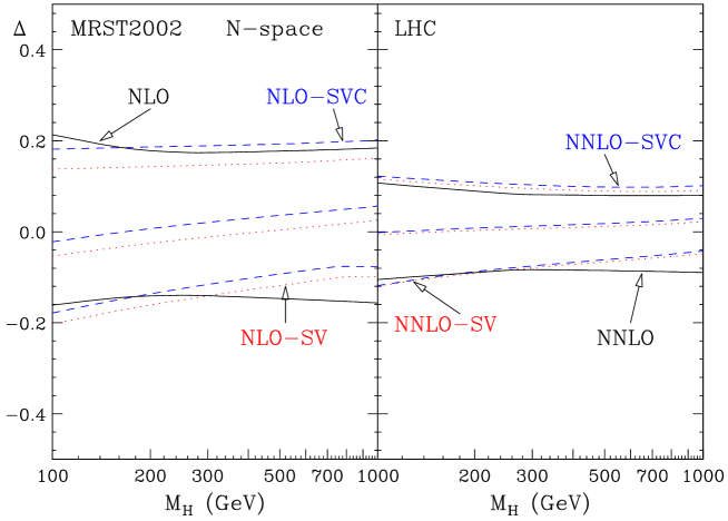
Figure 1: The SV (dotted lines) and SVC (dashed lines) approximations in $N$-space versus the exact results (solid lines) at the LHC (${\sqrt{s}}=14$ TeV).

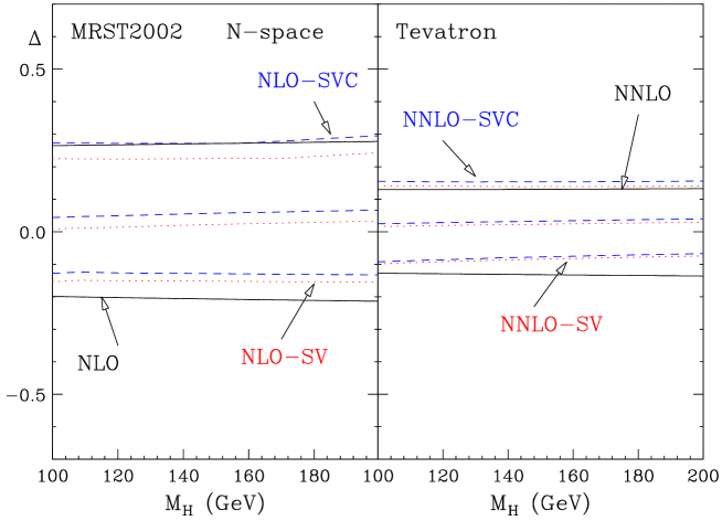
Figure 2: The SV (dotted lines) and SVC (dashed lines) approximations in $N$-space versus the exact results (solid lines) at the Tevatron (${\sqrt{s}}=1.96$ TeV).

The central curves are obtained by fixing $\mu_{F}=\mu_{R}=M_{H}$. The bands are obtained by varying $\mu_{F}$ and $\mu_{R}$ simultaneously and independently in the range $0.5M_{H}\leq\mu_{F},\mu_{R}\leq 2M_{H}$ with the constraint $0.5\leq\mu_{F}/\mu_{R}\leq 2$.

Here and in the following, we use the MRST2002 [50] set of parton distributions, which includes (approximated [45, 46, 51]) NNLO parton distributions. The parton densities and QCD coupling are evaluated at each corresponding order, by using 1-loop $\alpha_{\mathrm{S}}$ at LO, 2-loop $\alpha_{\mathrm{S}}$ at NLO and 3-loop $\alpha_{\mathrm{S}}$ at NNLO. The corresponding values of $\alpha_{\mathrm{S}}(M_{Z})$ are 0.130, 0.1197, 0.1154, at 1-loop, 2-loop and 3-loop order, respectively.

As can be observed from Figs. 1 and 2, the SV and SVC approximations in $N$-space agree very well with the exact NLO and NNLO calculations. Moreover, the differences between the approximated and exact results are substantially smaller than the effects produced by the scale variations in the exact results at each fixed order. A sizeable part of these small differences can be understood from the fact that in the approximation only the $gg$ channel contribution is included, thus neglecting the negative contribution from the $qg$ channel, which incidentally is also well approximated by its leading collinear behaviour at large $N$. The very small numerical difference between the SV and SVC approximations is consistent with the fact that they formally differ by $1/N$ suppressed terms, thus again confirming the consistency of the approximation based on the large-$N$ expansion.

The soft approximation, as well as the SV and SVC approximations, can also be defined in $x$ space. In this formulation, the large logarithm to be considered is $\ln(1-x)$, instead of $\ln N$. It is easy to go from one formulation to the other by Mellin transform. For example (see e.g. Eqs. (21)–(23) and Appendix A), one goes from the $x$-space formulae to the $N$-space ones by performing a Mellin transformation and discarding all $1/N$ suppressed terms, and all terms that are subleading (in the large-$N$ limit) with respect to the logarithmic accuracy of the initial $x$-space formulae. Thus, $x$-space and $N$-space formulae generally differ by terms that are formally subleading.

It has been shown in Ref. [39] that large subleading terms arise in the $x$-space formulation of the resummation program. These subleading terms grow factorially with the order of the perturbative expansion. Their factorial growth is not related to renormalons or Landau singularities. These terms are rather an artefact of the $x$-space approximation, which mistreats the kinematical constraint of energy conservation, and they should not be present in the exact theory. As a consequence of the factorial growth of these terms, all-order resummation cannot systematically be defined (implemented) in $x$-space, since the series of LL, NLL, NNLL, $\dots$ terms are separately divergent. It is therefore interesting to compare the $x$-space and $N$-space approximations for the first few exactly known orders.

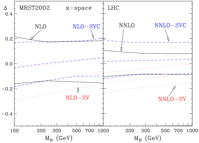
Figure 3: The SV-$x$ (dotted lines) and SVC-$x$ (dashed lines) approximations versus the exact results (solid lines) at the LHC (${\sqrt{s}}=14$ TeV).

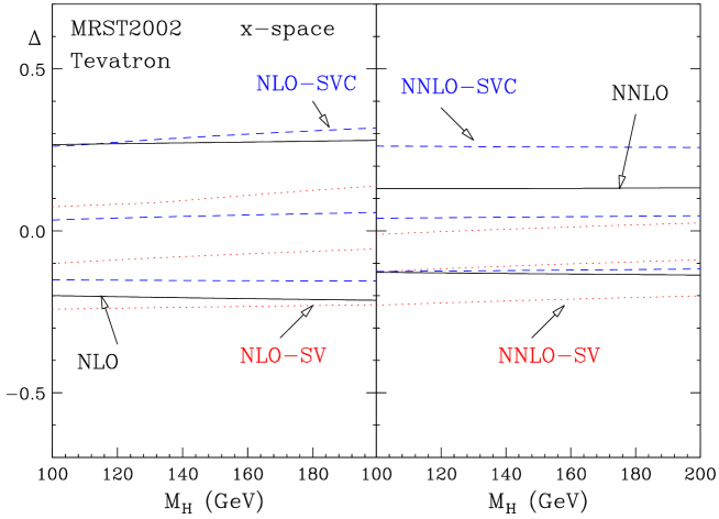
Figure 4: The SV-$x$ (dotted lines) and SVC-$x$ (dashed lines) approximations versus the exact results (solid lines) at the Tevatron (${\sqrt{s}}=1.96$ TeV).

At NLO, the $x$-space soft-virtual contribution (called SV-$x$ approximation, here) to the gluon coefficient function $G_{gg}^{(1)}$ in Eq. (2) is

$$G_{gg}^{(1)\,{\mbox{\footnotesize SV-$x$}}}(z;M_{H}^{2}/\mu_{R}^{2};M_{H}^{2}/\mu_{F}^{2}) =\delta(1-z)\left(\frac{11}{2}+6\zeta(2)+\frac{33-2N_{f}}{6}\ln\frac{\mu_{R}^{2}}{\mu_{F}^{2}}\right)$$

$$+\,6\,{\cal D}_{0}(z)\,\ln\frac{M_{H}^{2}}{\mu_{F}^{2}}+12\,{\cal D}_{1}(z)\;.$$ (59)

The same approximation can be defined at NNLO, and the corresponding contribution to the gluon coefficient function $G_{gg}^{(2)}(z)$ has the form

$$G_{gg}^{(2)\,{{\mbox{\footnotesize SV-$x$}}}}(z;M_{H}^{2}/\mu_{R}^{2},M_{H}^{2}/\mu_{F}^{2})=\delta(1-z)\;\delta G^{(2)}+{\cal D}_{0}\;G_{0}^{(2)}+{\cal D}_{1}\;G_{1}^{(2)}+{\cal D}_{2}\;G_{2}^{(2)}+{\cal D}_{3}\;G_{3}^{(2)}\;,$$ (60)

where the coefficients $\delta G^{(2)},G_{0}^{(2)},G_{1}^{(2)}$ and $G_{3}^{(2)}$ were computed in Refs. [8, 9] (these coefficients can be found in Eq. (2.13) of Ref. [8]).

After including the leading collinear logarithmic contributions, the $x$-space soft-virtual-collinear (SVC-$x$) approximation is defined [8] by

$$G_{gg}^{(1)\,{{\mbox{\footnotesize SVC-$x$}}}}(z;M_{H}^{2}/\mu^{2}_{R};M_{H}^{2}/\mu^{2}_{F})=G_{gg}^{(1)\,{{\mbox{\footnotesize SV-$x$}}}}(z;M_{H}^{2}/\mu^{2}_{R};M_{H}^{2}/\mu^{2}_{F})-12\,\ln(1-z)\;\;,$$ (61)

$$G_{gg}^{(2)\,{{\mbox{\footnotesize SVC-$x$}}}}(z;M_{H}^{2}/\mu^{2}_{R};M_{H}^{2}/\mu^{2}_{F})=G_{gg}^{(2)\,{{\mbox{\footnotesize SV-$x$}}}}(z;M_{H}^{2}/\mu^{2}_{R};M_{H}^{2}/\mu^{2}_{F})-72\,\ln^{3}(1-z)\;\;.$$ (62)

Figures 3 and 4 are obtained in the same way as Figs. 1 and 2, except for the use of the SV-$x$ and SVC-$x$ approximations instead of the analogous $N$-space approximations. These figures show that the bulk of the fixed-order radiative corrections is given by the SV-$x$ and SVC-$x$ approximations, as observed in Refs. [8, 16]. However, comparing Figs. 3 and 4 with Figs. 1 and 2, we also see that the $x$-space approximations are worse than the $N$-space ones. Furthermore, the difference between the SV-$x$ and SVC-$x$ approximations (which is formally suppressed by a power of $(1-z)$) is considerably larger than the difference between the SV-$N$ and SVC-$N$ approximations (which is formally suppressed by a power of $1/N$).

The lower quality of the $x$-space approximations at NLO and NNLO can have two different origins. First, the typical value $\langle 1-z\rangle$ of the distance from the partonic threshold, which is the parameter that formally controls the large-$x$ expansion, can be quantitatively larger than the typical value $\langle 1/N\rangle$ of the analogous expansion parameter in the $N$-space approach. Second, the numerical coefficients in the $x$-space expansion formulae can be larger than those in the $N$-space expansion formulae, as is the case at very high perturbative orders, because of the presence of factorially-growing subleading terms in the $x$-space approach. Of course, given the few orders available in the perturbative expansion, it is very difficult to explicitly check for the presence or absence of these factorial terms. We conclude, however, that these results provide no justification for estimating terms of still higher order through the soft-gluon approximation in the $x$-space approach.

4.2 Numerical relevance of the resummation

Before moving to the phenomenological results for soft-gluon resummation in Higgs production at the LHC and at the Tevatron, it is interesting to study the main features of the resummed coefficient function. This is better done in $N$-space, since both the resummed and fixed-order coefficient functions in $x$-space are distributions, and their numerical impact is therefore more difficult to assess.

To directly observe the effect of the exponentiation, we fix the coupling constant at $\alpha_{\mathrm{S}}=0.1$, the Higgs mass at $M_{H}=150$ GeV, and the scales at $\mu_{F}=\mu_{R}=M_{H}$. Figure 5 shows the $N$-moments, $G_{gg,\,N}$, of the resummed (left-hand side) and fixed-order (right-hand side) gluon coefficient function. The fixed-order coefficient function (see Eq. (8)) is evaluated at LO, NLO and NNLO. The resummed coefficient function (see Eq. (3.1)) is evaluated at LL (i.e. including the function $g_{H}^{(1)}$), NLL (i.e. including also the function $g_{H}^{(2)}$ and the coefficient $C_{gg}^{(1)}$) and NNLL (i.e. including also the function $g_{H}^{(3)}$ and the coefficient $C_{gg}^{(2)}$) order. At large values of $N$, there is a noticeable improvement in the convergence of the perturbative expansion once the resummation is performed. Indeed, the ratio between NNLL and NLL results is considerably smaller than the one between NLL and LL results. On the contrary, fixed-order results show an increasing ratio between two successive orders, which is due to the appearance of new and large $\ln^{(i)}N$ terms in the fixed-order expansion. Note, however, that we do not anticipate very large resummation effects on Higgs boson production at the LHC and the Tevatron. In fact, we know [8]–[13] that the ratio between the NNLO and LO cross sections does not exceed a factor of about 3 at these hadron colliders. From inspection of the right-hand side of Fig. 5, we thus expect that the Higgs boson cross section at LHC and Tevatron energies is mainly sensitive to the gluon coefficient function at moderate values of $N$.

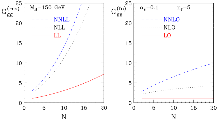
Figure 5: $N$-dependence of resummed (left-hand side) and fixed-order (right-hand side) gluon coefficient functions for Higgs production ($M_{H}=150$ GeV) with fixed coupling constant $\alpha_{\mathrm{S}}=0.1$.

5 Phenomenological results

5.1 Resummed cross section

We use soft-gluon resummation in $N$-space at the parton level (i.e. at the level of the partonic coefficient function $G_{ab}$) to introduce an improved (resummed) hadronic cross section $\sigma^{\rm(res)}(s,M_{H}^{2})$, which is obtained by inverse Mellin transformation (see Eq. (20)) as follows:

$$\sigma^{\rm(res)}(s,M_{H}^{2}) =\sigma^{(0)}\;\int_{C_{MP}-i\infty}^{C_{MP}+i\infty}\;\frac{dN}{2\pi i}\;\left(\frac{M_{H}^{2}}{s}\right)^{-N+1}\;f_{g/h_{1},\,N}(\mu_{F}^{2})\;f_{g/h_{2}\,N}(\mu_{F}^{2})$$

$$\times\left[\;{G}_{gg,\,N}^{\rm(res)}(\alpha_{\mathrm{S}}(\mu_{R}^{2}),M_{H}^{2}/\mu_{R}^{2};M_{H}^{2}/\mu_{F}^{2})-\left({G}_{gg,\,N}^{\rm(res)}(\alpha_{\mathrm{S}}(\mu_{R}^{2}),M_{H}^{2}/\mu_{R}^{2};M_{H}^{2}/\mu_{F}^{2})\right)_{\rm(f.o.)}\,\right]$$

$$+\sigma^{\rm(f.o.)}(s,M_{H}^{2})\;\;,$$ (63)

where $\sigma^{\rm(f.o.)}(s,M_{H}^{2})$ is the Higgs boson hadronic cross section at a given fixed order (f.o. = LO, NLO, NNLO), ${G}_{gg,\,N}^{\rm(res)}$ is given in Eq. (3.1), and $\left({G}_{gg,\,N}^{\rm(res)}\right)_{\rm(f.o.)}$ represents its perturbative truncation at the same fixed order in $\alpha_{\mathrm{S}}(\mu_{R}^{2})$. Thus, because of the subtraction in the square bracket on the right-hand side, Eq. (5.1) exactly reproduces the fixed-order results and resums soft-gluon effects beyond those fixed orders up to a certain logarithmic accuracy.

In the following subsections, we present numerical results for the resummed cross section $\sigma^{\rm(res)}(s,M_{H}^{2})$ at LL, NLL and NNLL accuracy. The resummed coefficient function ${G}_{gg,\,N}^{\rm(res)}$ in Eq. (5.1) is evaluated from the expressions in Eqs. (3.1)–(29): at LL accuracy we include the function $g_{H}^{(1)}$; at NLL accuracy we include also the function $g_{H}^{(2)}$ and the coefficient $C_{gg}^{(1)}$; at NNLL accuracy we include also $g_{H}^{(3)}$ and $C_{gg}^{(2)}$. Although they are briefly denoted as N^kLL $(k=0,1,2)$, the resummed results are always matched to the corresponding fixed order (f.o. = N^kLO) according to Eq. (5.1), i.e. LL is matched to LO, NLL to NLO and NNLL to NNLO.

Unless otherwise stated, cross sections are computed using sets of parton distributions, with densities and QCD coupling evaluated at each corresponding order, by using 1-loop $\alpha_{\mathrm{S}}$ at LO (LL), 2-loop $\alpha_{\mathrm{S}}$ at NLO (NLL), and 3-loop $\alpha_{\mathrm{S}}$ at NNLO (NNLL).

We recall that the hard coefficient function $G_{ab}$ is evaluated in the large-$M_{t}$ approximation, whereas the exact dependence on the masses $M_{t}$ and $M_{b}$ of the top and bottom quark is included in the Born-level cross section $\sigma^{(0)}$. We use $M_{t}=176$ GeV and $M_{b}=4.75$ GeV.

The inverse Mellin transformation in Eq. (5.1) involves an integral in the complex $N$ plane. When the $N$-moments ${G}_{gg,\,N}$ are evaluated at a fixed perturbative order, they are analytic functions in a right half-plane of the complex variable $N$. In this case, the constant $C_{MP}$ that defines the integration contour has to be chosen in this half-plane, that is, on the right of all the possible singularities of the $N$-moments.

When ${G}_{gg,\,N}$ is evaluated in resummed perturbation theory, the resummed functions $g_{H}^{(n)}(\lambda)$ in Eqs. (41)–(43) are singular at the point $\lambda=1/2$, which corresponds to $N=N_{L}=\exp(1/2b_{0}\alpha_{\mathrm{S}}(\mu_{R}^{2}))$ (i.e. $N_{L}\sim M_{H}/\Lambda_{QCD}$). These singularities, which are related to the divergent behaviour of the perturbative running coupling $\alpha_{\mathrm{S}}$ near the Landau pole, signal the onset of non-perturbative phenomena at very large values of $N$ or, equivalently, in the region very close to threshold. We deal with these singularities by using the Minimal Prescription introduced in Ref. [39]. In the evaluation of the inverse Mellin transformation in Eq. (5.1), the constant $C_{MP}$ is chosen in such a way that all singularities in the integrand are to the left of the integration contour, except for the Landau singularity at $N=N_{L}$, that should lie to the far right. The results obtained by using this prescription converge asymptotically to the perturbative series and do not introduce (unjustified) power corrections of non-perturbative origin. These corrections are certainly present in physical cross sections, but their effect is not expected to be sizeable, as long as $M_{H}$ is sufficiently perturbative and $\tau_{H}=M_{H}^{2}/s$ is sufficiently far from the hadronic threshold, as is the case in Higgs boson production at the Tevatron and the LHC.

The resummed cross section in Eq. (5.1) can equivalently be rewritten as

$$\sigma^{\rm(res)}(s,M_{H}^{2})=\sigma^{\rm(SV)}(s,M_{H}^{2})+\sigma^{\rm(match.)}(s,M_{H}^{2})\;\;,$$ (64)

where $\sigma^{\rm(SV)}$ denotes the contribution obtained by Mellin inversion of ${G}_{gg,\,N}^{\rm(res)}$, while the matching contribution $\sigma^{\rm(match.)}$ denotes the fixed-order cross section minus the corresponding fixed-order truncation of the soft-gluon resummed terms. As can easily be argued from the numerical results in Sect. 4.1, $\sigma^{\rm(SV)}$ gives the bulk of the QCD radiative corrections to the Higgs boson cross section at the Tevatron and the LHC. The order of magnitude of the relative contribution from $\sigma^{\rm(match.)}$ can be estimated from the size of the ratio $\Delta$ (see the definition in Eq. (56)) in Figs. 1 and 2: it is of ${\cal O}(10\%)$ and of ${\cal O}(1\%)$ at NLO and NNLO, respectively. Thus, the fixed-order cross section $\sigma^{\rm(match.)}$ quantitatively behaves as naively expected from a power series expansion whose expansion parameter is $\alpha_{\mathrm{S}}\sim 0.1$. We expect that the currently unknown (beyond NNLO) corrections to $\sigma^{\rm(match.)}$ have no practical quantitative impact on the QCD predictions for Higgs boson production at the Tevatron and the LHC.

We note that the predictions we are going to present regard the production of an on-shell Higgs boson. Therefore they are directly applicable at low values of $M_{H}$, where the small-width approximation is valid. At high values of $M_{H}$, corrections due to finite-width effects have to be implemented.

5.2 LHC

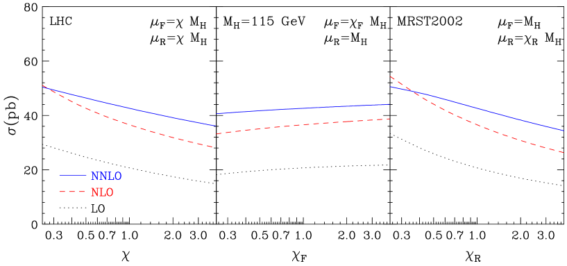
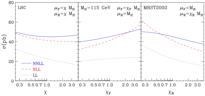
Figure 6: Scale dependence of the Higgs production cross section at the LHC for $M_{H}=115$ GeV at a) (upper) LO, NLO, NNLO and b) (lower) LL, NLL, NNLL accuracy.

In this subsection we study the phenomenological impact of soft-gluon resummation on the production of the SM Higgs boson at the LHC. The cross sections are computed using the MRST2002 set of parton distributions [50], with densities and QCD coupling evaluated at each corresponding order, as stated in Sect. 5.1 and done in Sect. 4.1.

We begin the presentation of our results by showing in Fig. 6 the scale dependence of the cross section for the production of a Higgs boson with $M_{H}=115$ GeV. The scale dependence is analysed by varying the factorization and renormalization scales around the default value $M_{H}$. The plot on the left corresponds to the simultaneous variation of both scales, $\mu_{F}=\mu_{R}=\chi\,M_{H}$, whereas the plot in the centre (right) corresponds to the variation of the factorization (renormalization) scale $\mu_{F}=\chi_{F}\,M_{H}$ ($\mu_{R}=\chi_{R}\,M_{H}$) by fixing the other scale at the default value $M_{H}$.

As expected from the QCD running of $\alpha_{\mathrm{S}}$, the cross sections typically decrease when $\mu_{R}$ increases around the characteristic hard scale $M_{H}$, at fixed $\mu_{F}=M_{H}$. In the case of variations of $\mu_{F}$ at fixed $\mu_{R}=M_{H}$, we observe the opposite behaviour. In fact, when $M_{H}=115$ GeV, the cross sections are mainly sensitive to partons with momentum fraction $x\sim 10^{-2}$, and in this $x$-range scaling violation of the parton densities is (moderately) positive. Varying the two scales simultaneously ($\mu_{F}=\mu_{R}$) leads to a compensation of the two different behaviours. As a result, the scale dependence is mostly driven by the renormalization scale, because the lowest-order contribution to the process is proportional to $\alpha_{\mathrm{S}}^{2}$, a (relatively) high power of $\alpha_{\mathrm{S}}$.

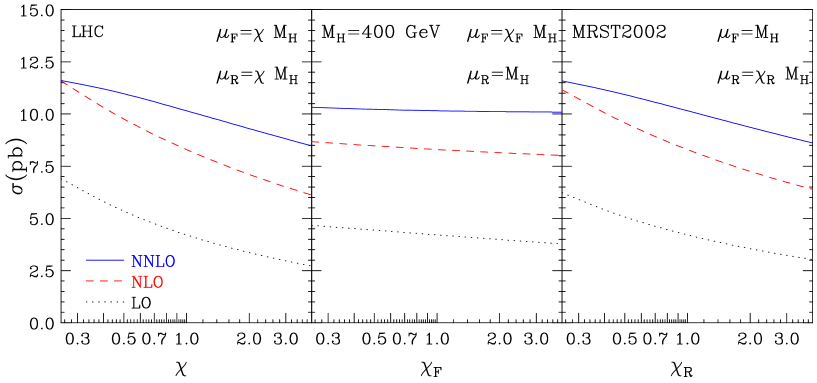
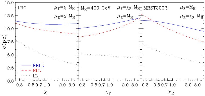
Figure 7: Scale dependence of the Higgs production cross section at the LHC for $M_{H}=400$ GeV at a) (upper) LO, NLO, NNLO and b) (lower) LL, NLL, NNLL accuracy.

Figure 6a shows that the scale dependence is reduced when higher-order corrections are included. When resummation effects are implemented (Fig. 6b), we typically observe a further (slight) reduction of the scale dependence, with the exception of the factorization-scale dependence at fixed $\mu_{R}=M_{H}$ that is marginally stronger after resummation. This suggests that the rather flat dependence on $\mu_{F}$ at NNLO can be an accidental effect, as also suggested by the fact that the $\mu_{F}$ dependence is much weaker than the $\mu_{R}$ dependence at each fixed order (LO, NLO, NNLO).

In Fig. 7, analogous results are plotted at a higher value, $M_{H}=400$ GeV, of the Higgs boson mass. The overall features of Figs. 6 and 7 are similar, although we notice that the improvement in the scale dependence when higher-order contributions are included is slightly better in Fig. 7 than in Fig. 6. An interesting difference between these two figures regards the $\mu_{F}$ dependence at fixed $\mu_{R}$. The LO, NLO, NNLO and LL results in Fig. 7 show that the corresponding cross sections (very) slightly decrease as $\mu_{F}$ increases around $M_{H}$. This is because, when increasing $M_{H}$ from $M_{H}=115$ GeV to $M_{H}=400$ GeV, the cross section is sensitive to partons with higher values of the momentum fraction $x$, so that scaling violation of the parton densities can become slightly negative. The fact that the parton densities are evaluated in an $x$-range where scaling violation changes sign is also suggested by the change in the slope of the $\mu_{F}$ dependence when going from LL to NLL and NNLL order.

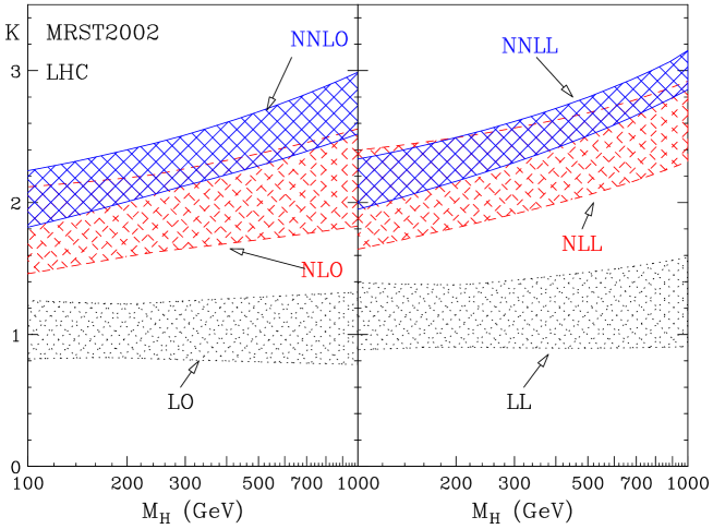
Figure 8: Fixed-order and resummed K-factors for Higgs production at the LHC.

The impact of higher-order corrections is sometimes presented through the $K$-factors, defined as the ratio of the cross section evaluated at each corresponding order over the LO result. The $K$-factors are shown in Fig. 8, where the bands are obtained, as in Sect. 4.1, by varying the scales $\mu_{R}$ and $\mu_{F}$ (simultaneously and independently) in the range $0.5M_{H}\leq\mu_{F},\mu_{R}\leq 2M_{H}$, with the constraint $0.5\leq\mu_{F}/\mu_{R}\leq 2$. The LO result that normalizes the $K$-factors is computed at the default scale $M_{H}$ in all cases. We see that the effect of the higher-order corrections increases with $M_{H}$. We also see that the soft-gluon resummation effects are more important at higher values of $M_{H}$. This is expected, since by increasing $M_{H}$ we are closer to the hadronic threshold, where soft-gluon effects are larger. When $M_{H}$ increases, the scale dependence after resummation is smaller than at the corresponding fixed orders. In the case of a light Higgs boson ($M_{H}\raisebox{-1.72218pt}{\hbox to0.0pt{$\,\sim\,$\hss}}\raisebox{1.72218pt}{$\,<\,$}200$ GeV), the NNLO K-factor is about 2.1–2.2, which corresponds to an increase of about $20\%$ with respect to the NLO K-factor. In this low-mass range, the effects of resummation are also moderate: at NNLL accuracy the central value of the cross section increases by about $6\%$ with respect to NNLO.

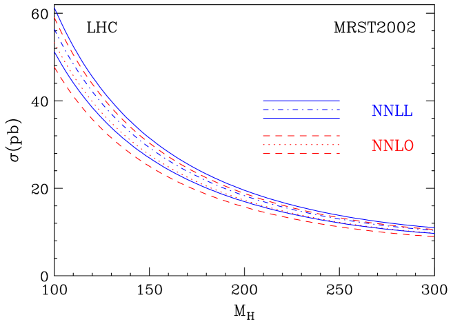
Figure 9: NNLL and NNLO cross sections at the LHC, using MRST2002 parton densities.

In Fig. 9 we plot the NNLO and NNLL cross sections, with the corresponding scale-dependence bands (computed as in Fig. 8), in the range $M_{H}=$100–300 GeV. The corresponding numerical results are given in Table 1, where $\sigma_{\rm min}$, $\sigma_{\rm max}$ and $\sigma_{\rm ref}$ correspond to the minimum, maximum and central values in the bands.

$M_{H}$	$\sigma^{NNLO}_{\rm min}$	$\sigma^{NNLO}_{\rm ref}$	$\sigma^{NNLO}_{\rm max}$	$\sigma^{NNLL}_{\rm min}$	$\sigma^{NNLL}_{\rm ref}$	$\sigma^{NNLL}_{\rm max}$
100	47.71	53.30	59.02	51.22	56.36	61.28
110	41.08	45.77	50.55	44.12	48.41	52.47
120	35.81	39.80	43.85	38.46	42.10	45.52
130	31.52	34.96	38.45	33.87	37.00	39.92
140	27.99	30.99	34.02	30.09	32.80	35.32
150	25.05	27.69	30.34	26.94	29.31	31.51
160	22.56	24.90	27.25	24.28	26.37	28.31
170	20.45	22.54	24.64	22.02	23.88	25.59
180	18.65	20.52	22.40	20.08	21.74	23.27
190	17.09	18.79	20.48	18.39	19.90	21.27
200	15.74	17.28	18.83	16.96	18.32	19.55
210	14.57	15.98	17.39	15.70	16.94	18.07
220	13.55	14.85	16.14	14.60	15.74	16.78
230	12.65	13.86	15.05	13.65	14.70	15.65
240	11.87	12.99	14.10	12.81	13.78	14.67
250	11.19	12.24	13.28	12.08	12.99	13.81
260	10.60	11.58	12.55	11.45	12.30	13.06
270	10.09	11.01	11.93	10.90	11.70	12.42
280	9.648	10.53	11.39	10.42	11.18	11.86
290	9.270	10.11	10.94	10.02	10.74	11.39
300	8.960	9.773	10.57	9.696	10.38	11.00

Table 1: NNLO and NNLL cross sections (in pb) at the LHC, using MRST2002 parton densities.

5.3 Tevatron

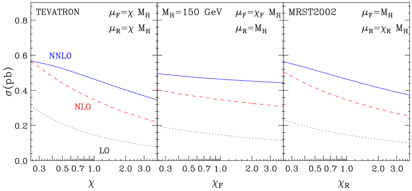
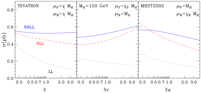
Figure 10: Scale dependence of the Higgs production cross section at the Tevatron for $M_{H}=150$ GeV at a) (upper) LO, NLO, NNLO and b) (lower) LL, NLL, NNLL accuracy.

Here we study the phenomenological impact of soft-gluon resummation on the production of the SM Higgs boson at the Tevatron Run II.

As in the previous subsection, we show in Fig. 10 the scale dependence of the fixed-order and resummed results. We use $M_{H}=150$ GeV. As in the LHC case, the cross sections typically decrease when $\mu_{R}$ increases around the characteristic hard scale $M_{H}$. Figure 10a shows that the fixed-order cross section decreases when $\mu_{F}$ increases at fixed $\mu_{R}$. This is not unexpected: at the Tevatron, the cross section is mainly sensitive to partons with $x\sim 0.05$–0.1, where the scaling violation is slightly negative. As in the LHC case, the $\mu_{F}$ dependence of the resummed results appears to be stronger than the $\mu_{F}$ dependence of the fixed-order results. The slope of the $\mu_{F}$ dependence changes sign in going from LL to NLL and NNLL order, as in the case of Fig. 7.

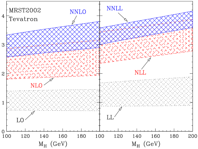
Figure 11: Fixed order and resummed K-factors for Higgs production at the Tevatron Run II ($\sqrt{s}=1.96$ TeV).

In Fig. 11 we plot the K-factor bands defined as in Fig. 8. We see that the impact of higher-order corrections at fixed $M_{H}$ is larger at the Tevatron than at the LHC. This is not unexpected: at the Tevatron, the Higgs boson is produced closer to the hadronic threshold and soft-gluon effects are therefore more sizeable. The NNLO K-factor is about 3–3.2, with an increase of about $40\%$ with respect to NLO. Correspondingly, also the resummation effects are larger: at NNLL they increase the NNLO cross section by about 12–15$\%$. The scale dependence of the NNLL result is smaller than at NNLO.

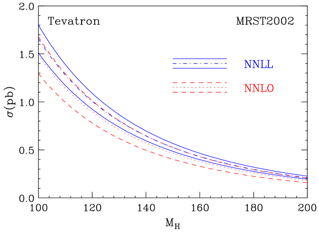
Figure 12: NNLL and NNLO cross sections at the Tevatron ($\sqrt{s}=1.96$ TeV), using MRST2002 parton densities.

In Fig. 12 we plot the NNLO and NNLL cross-section bands, obtained as in Figs. 8 and 11, in the mass range $M_{H}=100$–200 GeV. The corresponding numerical results are given in Table 2.

$M_{H}$	$\sigma^{NNLO}_{\rm min}$	$\sigma^{NNLO}_{\rm ref}$	$\sigma^{NNLO}_{\rm max}$	$\sigma^{NNLL}_{\rm min}$	$\sigma^{NNLL}_{\rm ref}$	$\sigma^{NNLL}_{\rm max}$
100	1.2946	1.4846	1.6783	1.5129	1.6568	1.8009
105	1.1335	1.3006	1.4701	1.3292	1.4535	1.5784
110	0.9970	1.1445	1.2936	1.1728	1.2808	1.3894
115	0.8804	1.0112	1.1429	1.0389	1.1331	1.2281
120	0.7803	0.8967	1.0135	0.9237	1.0062	1.0898
125	0.6939	0.7978	0.9017	0.8240	0.8965	0.9704
130	0.6190	0.7120	0.8048	0.7373	0.8013	0.8668
135	0.5537	0.6373	0.7204	0.6615	0.7182	0.7766
140	0.4967	0.5719	0.6465	0.5951	0.6455	0.6976
145	0.4466	0.5145	0.5817	0.5367	0.5815	0.6282
150	0.4025	0.4639	0.5246	0.4850	0.5251	0.5670
155	0.3635	0.4193	0.4742	0.4393	0.4752	0.5130
160	0.3290	0.3797	0.4295	0.3988	0.4310	0.4651
165	0.2984	0.3445	0.3898	0.3627	0.3917	0.4226
170	0.2712	0.3132	0.3544	0.3305	0.3566	0.3847
175	0.2469	0.2852	0.3228	0.3017	0.3253	0.3509
180	0.2251	0.2602	0.2946	0.2758	0.2972	0.3206
185	0.2056	0.2378	0.2693	0.2526	0.2720	0.2933
190	0.1881	0.2177	0.2465	0.2317	0.2493	0.2688
195	0.1724	0.1996	0.2261	0.2129	0.2289	0.2469
200	0.1582	0.1832	0.2076	0.1959	0.2105	0.2270

Table 2: NNLO and NNLL cross sections (in pb) at the Tevatron ($\sqrt{s}=1.96$ TeV), using MRST2002 parton densities.

5.4 Uncertainties on Higgs production cross section

In this subsection we would like to discuss the various sources of QCD uncertainty that still affect the Higgs production cross section, focusing on the low-$M_{H}$ region ($M_{H}\raisebox{-1.72218pt}{\hbox to0.0pt{$\,\sim\,$\hss}}\raisebox{1.72218pt}{$\,<\,$}200$ GeV). The uncertainty basically has two origins: the one coming from still unknown perturbative QCD contributions to the coefficient function $G_{ab}$ in Eq. (2), and the one originating from our limited knowledge of the parton distributions.

Uncalculated higher-order QCD radiative corrections are the most important source of uncertainty on the coefficients $G_{ab}$. A method, which is customarily used in perturbative QCD calculations, to estimate their size is to vary the renormalization and factorization scales around the hard scale $M_{H}$. In general, this procedure can only give a lower limit on the ‘true’ uncertainty. This is well demonstrated by Figs. 8 and 11, which show no overlap between the LO and NLO (or, LL and NLL) bands. However, the NLO and NNLO bands and, also, the NNLO and NNLL bands do overlap. Furthermore, the central value of the NNLL bands lies inside the corresponding NNLO bands. This gives us confidence in using scale variations to estimate the uncertainty at NNLO and at NNLL order.

Performing scale variations as in Figs. 8, 9, 11 and 12, from the numerical results in Tables 1 and 2, we find the following results. At the LHC, the NNLO scale dependence ranges from about $\pm 10\%$ when $M_{H}=120$ GeV, to about $\pm 9\%$ when $M_{H}=200$ GeV. At NNLL order, it is about $\pm 8\%$ when $M_{H}\raisebox{-1.72218pt}{\hbox to0.0pt{$\,\sim\,$\hss}}\raisebox{1.72218pt}{$\,<\,$}200$ GeV. At the Tevatron, when $M_{H}\raisebox{-1.72218pt}{\hbox to0.0pt{$\,\sim\,$\hss}}\raisebox{1.72218pt}{$\,<\,$}200$ GeV, the NNLO scale dependence is about $\pm 13\%$, whereas the NNLL scale dependence is about $\pm 8\%$.

Another method to estimate the size of higher-order corrections is to compare the results at the highest available order with those at the previous order. Considering the differences between the NNLO and NNLL cross sections, we obtain results that are consistent with the uncertainty estimated from scale variations.

We have also considered other possible sources of higher-order uncertainty. The NNLL coefficient $A^{(3)}$ is not yet exactly known (see Eq. (40) and the accompanying comment). One can thus wonder which is the numerical impact of $A^{(3)}$ in the calculation. We have investigated the numerical effect of $A^{(3)}$ by comparing the full NNLL result with the same result obtained by setting $A^{(3)}=0$. The differences are below $1\%$, allowing us to conclude that the uncertainty from $A^{(3)}$ can safely be neglected. Similar conclusions can be drawn about the inclusion of the dominant collinear contributions (see Eq. (50)) in the resummed formula. At NNLL order, it gives an effect below $1\%$, in agreement with the fact that collinear logarithmic contributions, which are formally suppressed by powers of $1/N$, give only a small correction to the dominant terms due to soft and virtual contributions (see Sect. 4).

A different and relevant source of perturbative QCD uncertainty comes from the use of the large-$M_{t}$ approximation in the computation of $G_{ab}$ beyond the LO. The comparison [6, 15] between the exact NLO cross section and the one obtained in the large-$M_{t}$ approximation (but rescaled with the full Born result, including its exact dependence on $M_{t}$ and $M_{b}$) shows that the approximation works well also for $M_{H}\raisebox{-1.72218pt}{\hbox to0.0pt{$\,\sim\,$\hss}}\raisebox{1.72218pt}{$\,>\,$}M_{t}$. This is not accidental. In fact, the higher-order contributions to the cross section are dominated by soft radiation, which is weakly sensitive to the mass of the heavy quark in the loop at the Born level. In other words, as for the size of the QCD radiative corrections, what matters is that the heavy-quark mass, $M_{t}$ is actually larger than the soft-gluon scale, $M_{H}/N$, rather than the Higgs boson scale $M_{H}$. This feature, i.e. the dominance of soft-gluon effects, persists at NNLO (see Sect. 4) and it is thus natural to assume that, having normalized our cross sections with the exact Born result, the uncertainty ensuing from the large-$M_{t}$ approximation should be of order of few per cent for $M_{H}\raisebox{-1.72218pt}{\hbox to0.0pt{$\,\sim\,$\hss}}\raisebox{1.72218pt}{$\,<\,$}200$ GeV, as it is at NLO.

Besides QCD radiative corrections, electroweak corrections also have to be considered. For a light Higgs, the ${\cal O}(G_{F}M_{t}^{2})$ dominant corrections in the large-$M_{t}$ limit have been computed and found to give a very small effect (well below $1\%$) [52].

The other independent and important source of theoretical uncertainty in the cross section is the one coming from parton distributions.

We start our discussion by considering NLO results. We have compared the MRST2002 NLO cross sections with the ones computed with CTEQ6 [53] and Alekhin [54] distributions. All three sets include a study of the effect of the experimental uncertainties in the extraction of the parton densities. At the LHC, we find that the CTEQ6M results are slightly larger than the MRST2002 ones, the differences decreasing from about $2\%$ at $M_{H}=100$ GeV to below $1\%$ at $M_{H}=200$ GeV. Alekhin’s results are instead slightly smaller than the MSRT2002 ones, the difference being below $3\%$ for $M_{H}\raisebox{-1.72218pt}{\hbox to0.0pt{$\,\sim\,$\hss}}\raisebox{1.72218pt}{$\,<\,$}200$ GeV. At the Tevatron, CTEQ6 (Alekhin) cross sections are smaller than the MRST2002 ones, the differences increasing from $6\%$ ($7\%$) to $10\%$ ($9\%$) when $M_{H}$ increases from $100$ GeV to $200$ GeV. These results are not unexpected, since in Higgs production at the Tevatron the gluon distribution is probed at larger values of $x$, where its (experimental) uncertainty is definitely larger. The cross section differences that we find at NLO are compatible with the experimental uncertainty on the NLO gluon luminosity quoted by the three groups, which is below about $\pm 5\%$ at the LHC and about $\pm 10\%$ at the Tevatron [50, 53, 54].

Throughout the paper we have used the MRST2002 set [50] as the reference set of parton distributions. The main motivation for this choice is that this set includes (approximated) NNLO densities, allowing a consistent study at NNLL (NNLO) accuracy. The CTEQ collaboration does not provide a NNLO set, and a complete, consistent comparison with MRST can therefore not be performed. In Ref. [54], a NNLO set of parton distributions (set A02 from here on) has been released. This set also includes an estimate of the corresponding uncertainties. We can thus perform a comparison with the MRST2002 results.

$M_{H}$	$\sigma^{NNLO}$	$\sigma^{NNLL}$
$100$	$57.52^{+0.93}_{-0.93}$	$60.95^{+1.00}_{-1.00}$
$110$	$48.97^{+0.77}_{-0.77}$	$51.81^{+0.82}_{-0.82}$
$120$	$42.29^{+0.64}_{-0.64}$	$44.82^{+0.68}_{-0.69}$
$130$	$36.99^{+0.54}_{-0.55}$	$39.17^{+0.58}_{-0.59}$
$140$	$32.59^{+0.46}_{-0.47}$	$34.55^{+0.50}_{-0.50}$
$150$	$28.94^{+0.40}_{-0.40}$	$30.74^{+0.43}_{-0.43}$
$160$	$25.91^{+0.35}_{-0.35}$	$27.52^{+0.38}_{-0.38}$

$M_{H}$	$\sigma^{NNLO}$	$\sigma^{NNLL}$
$170$	$23.35^{+0.31}_{-0.31}$	$24.75^{+0.34}_{-0.33}$
$180$	$21.17^{+0.28}_{-0.28}$	$22.42^{+0.30}_{-0.30}$
$190$	$19.29^{+0.25}_{-0.25}$	$20.44^{+0.27}_{-0.27}$
$200$	$17.65^{+0.23}_{-0.23}$	$18.76^{+0.25}_{-0.25}$
$210$	$16.25^{+0.21}_{-0.21}$	$17.28^{+0.23}_{-0.23}$
$220$	$15.03^{+0.20}_{-0.20}$	$15.98^{+0.21}_{-0.21}$
$230$	$13.96^{+0.18}_{-0.18}$	$14.84^{+0.19}_{-0.19}$

$M_{H}$	$\sigma^{NNLO}$	$\sigma^{NNLL}$
$240$	$13.04^{+0.17}_{-0.17}$	$13.86^{+0.18}_{-0.18}$
$250$	$12.23^{+0.16}_{-0.16}$	$13.00^{+0.17}_{-0.17}$
$260$	$11.53^{+0.16}_{-0.16}$	$12.26^{+0.16}_{-0.16}$
$270$	$10.92^{+0.15}_{-0.15}$	$11.62^{+0.16}_{-0.16}$
$280$	$10.39^{+0.15}_{-0.15}$	$11.05^{+0.15}_{-0.15}$
$290$	$9.939^{+0.14}_{-0.14}$	$10.57^{+0.15}_{-0.15}$
$300$	$9.562^{+0.14}_{-0.14}$	$10.16^{+0.15}_{-0.15}$

Table 3: NNLO and NNLL cross sections (in pb) at the LHC ($\mu_{F}=\mu_{R}=M_{H}$) using the parton distributions of Ref. [54].

$M_{H}$	$\sigma^{NNLO}$	$\sigma^{NNLL}$
$100$	$1.378^{+0.041}_{-0.041}$	$1.548^{+0.043}_{-0.042}$
$105$	$1.203^{+0.038}_{-0.038}$	$1.347^{+0.039}_{-0.039}$
$110$	$1.054^{+0.035}_{-0.035}$	$1.181^{+0.037}_{-0.036}$
$115$	$0.9280^{+0.033}_{-0.032}$	$1.042^{+0.034}_{-0.034}$
$120$	$0.8194^{+0.030}_{-0.030}$	$0.9227^{+0.031}_{-0.032}$
$125$	$0.7259^{+0.028}_{-0.028}$	$0.8191^{+0.029}_{-0.029}$
$130$	$0.6445^{+0.026}_{-0.026}$	$0.7292^{+0.027}_{-0.027}$

$M_{H}$	$\sigma^{NNLO}$	$\sigma^{NNLL}$
$135$	$0.5740^{+0.024}_{-0.024}$	$0.6503^{+0.026}_{-0.025}$
$140$	$0.5135^{+0.023}_{-0.023}$	$0.5816^{+0.024}_{-0.024}$
$145$	$0.4604^{+0.021}_{-0.021}$	$0.5210^{+0.023}_{-0.022}$
$150$	$0.4136^{+0.020}_{-0.020}$	$0.4686^{+0.021}_{-0.021}$
$155$	$0.3723^{+0.019}_{-0.019}$	$0.4231^{+0.020}_{-0.020}$
$160$	$0.3357^{+0.018}_{-0.017}$	$0.3831^{+0.019}_{-0.019}$
$165$	$0.3032^{+0.017}_{-0.016}$	$0.3471^{+0.018}_{-0.017}$

$M_{H}$	$\sigma^{NNLO}$	$\sigma^{NNLL}$
$170$	$0.2741^{+0.015}_{-0.015}$	$0.3142^{+0.016}_{-0.016}$
$175$	$0.2483^{+0.014}_{-0.014}$	$0.2841^{+0.015}_{-0.015}$
$180$	$0.2253^{+0.014}_{-0.014}$	$0.2577^{+0.015}_{-0.015}$
$185$	$0.2054^{+0.013}_{-0.013}$	$0.2353^{+0.014}_{-0.014}$
$190$	$0.1877^{+0.012}_{-0.012}$	$0.2157^{+0.013}_{-0.013}$
$195$	$0.1716^{+0.011}_{-0.011}$	$0.1981^{+0.012}_{-0.012}$
$200$	$0.1572^{+0.011}_{-0.011}$	$0.1818^{+0.012}_{-0.012}$

Table 4: NNLO and NNLL cross sections (in pb) at the Tevatron ($\mu_{F}=\mu_{R}=M_{H}$) using the parton distributions of Ref. [54].

In Table 3 (Table 4) we report the NNLO and NNLL cross sections (computed with $\mu_{F}=\mu_{R}=M_{H}$) obtained at the LHC (Tevatron) by using the set A02 of parton distributions. We also report the corresponding errors, computed by using the dispersion array of the A02 sets. Comparing Tables 3 and 4 with the corresponding central results in Tables 1 and 2, we see that there are relatively large differences that cannot be accounted for by the errors provided in the A02 set. At the LHC the cross section is larger than the one computed with the MRST2002 set, and the difference goes from about $8\%$ at low masses to about $2\%$ at $M_{H}=200$ GeV. At the Tevatron the cross section is lower than that using MRST2002, with a difference that ranges from about $7\%$ at low $M_{H}$ to about $14\%$ at $M_{H}=200$ GeV.

These differences can be better understood by looking at Figs. 13 and 14, where a comparison of Alekhin (with errors) and MSRT2002 luminosities is presented. Comparing Tables 1, 2, 3 and 4 with Figs. 13 and 14, we see that the differences in the cross sections are basically due to differences in the NNLO gluon–gluon luminosity. Moreover, Figs. 13 and 14 show that the differences between the luminosities are typically larger than the estimated uncertainty of experimental origin. In particular, the differences between the $gg$ luminosities appear to increase with the perturbative order (i.e. going from LO to NLO and to NNLO).

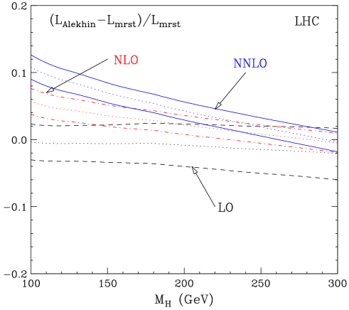
Figure 13: Comparison of A02 and MRST2002 gg luminosities at the LHC.

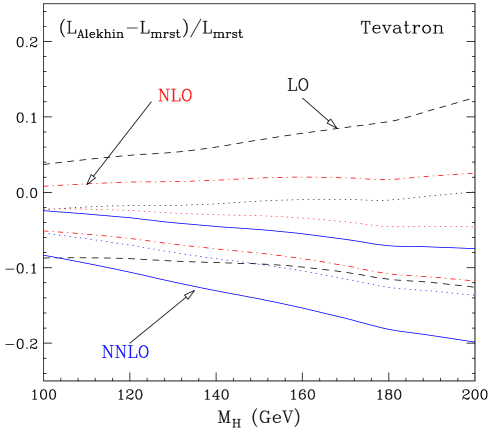
Figure 14: Comparison of A02 and MRST2002 gg luminosities at the Tevatron.

We are not able to pin down the origin of these differences. References [50] and [54] use the same (though approximated) NNLO evolution kernels, but the MRST2002 set is based on a fit of deep-inelastic scattering (DIS), DY and Tevatron jet data, whereas the A02 set is obtained through a fit to DIS data only.

From the above discussion, we conclude that the theoretical uncertainties of perturbative origin in the calculation of the Higgs production cross section, after inclusion of both NNLO corrections and soft-gluon resummation at the NNLL level, are below 10% in the low-mass range. However, it is also apparent that there are uncertainties in the (available) parton densities alone that can reach values larger than 10%, and that are not fully understood at the moment. Improvements of these aspects may only come from better understanding of parton density determinations, and are therefore totally unrelated to the calculation presented in this work.

6 Conclusions

In this work we have presented a next-to-next-to-leading resummation of soft-gluon effects in the gluon fusion cross section for Higgs production. Furthermore, we have supplemented our resummed result with available fixed-order (up to NNLO) calculations. We have presented a phenomenological study of the Higgs cross sections at the LHC and the Tevatron, and showed that, once problems with parton density determinations are overcome, a theoretical precision of about 10% in the predicted cross section can be attained.

The impact of the NNLL corrections included in this work was found to be modest in the case of light-Higgs production at the LHC. The NNLL corrections are more significant at the Tevatron, and allow us to reduce the theoretical error band at the same precision level as at the LHC. We believe that our results add much confidence in the predicted cross sections for the following reason. The pattern of radiative corrections from the NNLL resummation, when truncated at fixed order, reproduces quite well the pattern from the exact fixed-order calculations. This adds confidence that the higher-order (beyond the NNLO level) radiative corrections arising from the NNLL treatment reflect the behaviour of the exact theory.

As a side product of this work, we have shown that the $N$-space formulation of the soft-gluon approximation is superior to the $x$-space one. In Ref. [39] it was shown that the $N$-space formulation of soft-gluon resummation should be used, since it avoids a gross violation of momentum conservation, which in turn leads to an unphysically large asymptotic growth of the coefficients of the perturbative expansion. In the present work, the better behaviour of the $N$-space approach has also been shown to hold in practice, when comparing known fixed-order results with the fixed-order expansion of the resummation formulae, up to the NNLO level.

Appendix A Appendix: $N$-moments of soft-gluon contributions

In this appendix we present a simple method to evaluate $N$-moments of soft-gluon contributions to arbitrary logarithmic accuracy.

We consider the $N$-moments $I_{n}(N)$ of the singular distributions ${\cal D}_{n}(z)$ defined in Eq. (13):

$$I_{n}(N)\equiv\int_{0}^{1}dz\;z^{N-1}{\cal D}_{n}(z)=\int_{0}^{1}dz\;\frac{z^{N-1}-1}{1-z}\;\ln^{n}(1-z)\;\;.$$ (65)

These $N$-moments were computed in Ref. [26]. It was shown that, in the large-$N$ limit, the leading and next-to-leading logarithmic terms ($\ln^{n+1}N$ and $\ln^{n}N$) arising from the integration over $z$ can straightforwardly be obtained by a very simple prescription. It is indeed sufficient [26] to replace the integrand weight $(z^{N-1}-1)$ by the approximation

$$z^{N-1}-1\simeq-\;\Theta(1-z-N_{0}/N)\;\;,$$ (66)

where $N_{0}=e^{-\gamma_{E}}$. In the following we show how this NLL prescription can be generalized to any logarithmic accuracy. The all-order generalization of Eq. (66) is given in Eq. (76) or, equivalently, in Eq. (77).

The $N$-moments in Eq. (65) can be evaluated as described in Ref. [26]. Using the following identity

$$\ln^{n}(1-z)=\lim_{\epsilon\rightarrow 0}\left(\frac{\partial}{\partial\epsilon}\right)^{n}(1-z)^{\epsilon}$$ (67)

to replace the logarithmic term in the integrand on the right-hand side of Eq. (65), we obtain

$$I_{n}(N)=\lim_{\epsilon\rightarrow 0}\left(\frac{\partial}{\partial\epsilon}\right)^{n}\left\{\frac{1}{\epsilon}\left[\frac{\Gamma(N)\;\Gamma(1+\epsilon)}{\Gamma(N+\epsilon)}-1\right]\right\}\;\;,$$ (68)

where $\Gamma(x)$ is the Euler $\Gamma$-function. The expression (68) can be used to evaluate $I_{n}(N)$ for any given value of $n$ without approximations of the dependence on $N$ [26].

We are interested in the large-$N$ behaviour of $I_{n}(N)$. Neglecting terms that are suppressed by powers of $1/N$ in the large-$N$ limit, we can use the approximation

$$\frac{\Gamma(N)}{\Gamma(N+\epsilon)}=e^{-\epsilon\ln N}\left[1+{\cal O}\left(\frac{1}{N}\right)\right]\;\;,$$ (69)

and we can rewrite Eq. (68) as

$$I_{n}(N)=\lim_{\epsilon\rightarrow 0}\left(\frac{\partial}{\partial\epsilon}\right)^{n}\left\{\frac{1}{\epsilon}\left[e^{-\epsilon\ln N}\Gamma(1+\epsilon)-1\right]\right\}+{\cal O}\left(\frac{1}{N}\right)\;\;.$$ (70)

Using the expression

$$\Gamma(1+\epsilon)=\exp\left\{-\gamma_{E}\;\epsilon+\sum_{n=2}^{+\infty}\left(-1\right)^{n}\frac{\zeta(n)}{n}\;\epsilon^{n}\right\}\;\;,$$ (71)

the term in the curly bracket of Eq. (70) can easily be expanded in powers of $\epsilon$. The result for $I_{n}(N)$ is thus a polynomial of degree $n+1$ in the large logarithm $\ln N$:

$$I_{n}(N) =\frac{(-1)^{n+1}}{n+1}\,(\ln N+\gamma_{E})^{n+1}+\frac{(-1)^{n-1}}{2}\;n\,\zeta(2)\;(\ln N+\gamma_{E})^{n-1}$$

$$+\sum_{k=0}^{n-2}\;a_{nk}\;(\ln N+\gamma_{E})^{k}+{\cal O}\!\left(\frac{1}{N}\right)\;\;,$$ (72)

where the coefficients $a_{nk}$ are combinations of powers of $\zeta(2),\zeta(3),\dots,\zeta(n+1)$ (see e.g. Table 1 in Ref. [26]).

As shown by Eq. (A) and pointed out in Ref. [26], the LL and NLL terms ($\ln^{n+1}N$ and $\ln^{n}N$) can straightforwardly be obtained from the definition of the $N$-moments in Eq. (65) by simply implementing the prescription in Eq. (66). To show how this NLL prescription can be generalized to any logarithmic accuracy, we consider the right-hand side of Eq. (70) and use the following formal identity:

$$e^{-\epsilon\ln N}\;\Gamma(1+\epsilon)=\Gamma\!\left(1-\frac{\partial}{\partial\ln N}\right)\;e^{-\epsilon\ln N}\;\;.$$ (73)

Then we can perform the $n$-th derivative with respect to $\epsilon$, and we obtain

$$I_{n}(N)=\Gamma\!\left(1-\frac{\partial}{\partial\ln N}\right)\frac{\left(-\ln N\right)^{n+1}}{n+1}+{\cal O}\left(\frac{1}{N}\right)\;\;.$$ (74)

This expression can be regarded as a replacement of Eq. (70) to compute the polynomial coefficients $a_{nk}$ in Eq. (A). Moreover, by noting that

$$\frac{\left(-\ln N\right)^{n+1}}{n+1}=-\int_{0}^{1-1/N}dz\;\frac{\ln^{n}(1-z)}{1-z}\;\;,$$ (75)

we shortly get the all-order generalization of Eq. (66). It is:

$$z^{N-1}-1 =-\;\Gamma\!\left(1-\frac{\partial}{\partial\ln N}\right)\;\Theta(1-z-1/N)+{\cal O}(1/N)$$ (76)

$$=-\;{\widetilde{\Gamma}}\!\left(1-\frac{\partial}{\partial\ln N}\right)\;\Theta(1-z-N_{0}/N)+{\cal O}(1/N)\;\;,$$ (77)

where we have also introduced the function ${\widetilde{\Gamma}}$ defined by

$${\widetilde{\Gamma}}(1+\epsilon)\equiv e^{\gamma_{E}\,\epsilon}\;\Gamma(1+\epsilon)=\exp\left\{\sum_{n=2}^{+\infty}\left(-1\right)^{n}\frac{\zeta(n)}{n}\;\epsilon^{n}\right\}\;\;.$$ (78)

Note that the equality between Eqs. (76) and (77) simply follows from $\Gamma={\widetilde{\Gamma}}\exp[\gamma_{E}N\partial/(\partial N)]$ and from the fact that the exponential of the differential operator acts as the rescaling $N\rightarrow\exp[\gamma_{E}]N=N/N_{0}$.

Although we have derived it by starting from Eq. (65), it is straightforward to show that the prescription (76) (or (77)) can be applied as follows

$$\int_{0}^{1}dz\,\frac{z^{N-1}-1}{1-z}\,F(\alpha_{\mathrm{S}},\ln(1-z))\!\! =-\,\Gamma\!\left(1-\frac{\partial}{\partial\ln N}\right)\int_{0}^{1-1/N}\;\frac{dz}{1-z}\;F(\alpha_{\mathrm{S}},\ln(1-z))+{\cal O}\!\left(\frac{1}{N}\right)$$

$$=-\,{\widetilde{\Gamma}}\!\left(1-\frac{\partial}{\partial\ln N}\right)\int_{0}^{1-N_{0}/N}\!\!\frac{dz}{1-z}\;F(\alpha_{\mathrm{S}},\ln(1-z))+{\cal O}\!\left(\frac{1}{N}\right)$$

to evaluate the $\ln N$-contributions arising from the integration of any soft-gluon function $F$ that has a generic perturbative expansion of the type

$$F(\alpha_{\mathrm{S}},\ln(1-z))=\sum_{k=1}^{+\infty}\alpha_{\mathrm{S}}^{k}\;\sum_{n=0}^{2k-1}F_{kn}\;\ln^{n}(1-z)\;\;.$$ (79)

The all-order differential operator $\Gamma$ (${\widetilde{\Gamma}}$) in Eq. (76) (Eq. (77)) is obviously defined only in a formal sense through Eq. (71) (Eq. (78)). However, such a definition is sufficient for any formal manipulation to all logarithmic orders. Moreover, it is also sufficient for any practical use at fixed and arbitrary logarithmic accuracy. Since each additional power of $\partial/(\partial\ln N)$ leads to terms that are suppressed by a power of $\ln N$, we can obtain all the terms up to a given (and arbitrary) logarithmic order by simply truncating the power series expansion of $\Gamma$ at the corresponding order in the logarithmic derivative. For example, using the truncation

$$\Gamma\!\left(1-\frac{\partial}{\partial\ln N}\right) =1+\gamma_{E}\frac{\partial}{\partial\ln N}+\frac{1}{2}\left(\gamma_{E}^{2}+\zeta(2)\right)\left(\frac{\partial}{\partial\ln N}\right)^{2}$$

$$+\frac{1}{6}\left(\gamma_{E}^{3}+3\gamma_{E}\,\zeta(2)+2\zeta(3)\right)\left(\frac{\partial}{\partial\ln N}\right)^{3}+\dots\;\;,$$ (80)

the first, second, third and fourth terms on the right-hand side lead to the LL, NLL, NNLL and N³LL contributions, respectively.

Appendix B Appendix: Equivalence between resummation formulae

Here we prove the equivalence between the two all-order representations (31) and (36) of the Sudakov radiative factor $\Delta_{N}^{H}$. In particular, we derive the relations between the functions $A(\alpha_{\mathrm{S}})$ and $D(\alpha_{\mathrm{S}})$ in Eq. (31) and the functions ${\widetilde{D}}(\alpha_{\mathrm{S}})$ and ${\widetilde{C}}_{gg}(\alpha_{\mathrm{S}})$ in Eq. (36). These relations are:

$${\widetilde{D}}(\alpha_{\mathrm{S}})=D(\alpha_{\mathrm{S}})+4\;\partial_{\alpha_{\mathrm{S}}}\;\Gamma_{2}(\partial_{\alpha_{\mathrm{S}}})\left[A(\alpha_{\mathrm{S}})-\frac{1}{4}\;\partial_{\alpha_{\mathrm{S}}}\;D(\alpha_{\mathrm{S}})\right]\;\;,$$ (81)

$${\widetilde{C}}_{gg}(\alpha_{\mathrm{S}}(M_{H}^{2}),M_{H}^{2}/\mu^{2}_{R}=1)=\exp\left\{-4\;\Gamma_{2}(\partial_{\alpha_{\mathrm{S}}})\left[A(\alpha_{\mathrm{S}})-\frac{1}{4}\;\partial_{\alpha_{\mathrm{S}}}\;D(\alpha_{\mathrm{S}})\right]\right\}\;\;,$$ (82)

where the differential operator $\partial_{\alpha_{\mathrm{S}}}$ is defined by

$$\partial_{\alpha_{\mathrm{S}}}\equiv-2\beta(\alpha_{\mathrm{S}})\;\alpha_{\mathrm{S}}\;\frac{\partial}{\partial\alpha_{\mathrm{S}}}\;\;,$$ (83)

$\beta(\alpha_{\mathrm{S}})$ is the QCD $\beta$-function,

$$\frac{d\ln\alpha_{\mathrm{S}}(\mu^{2})}{d\ln\mu^{2}}=\beta(\alpha_{\mathrm{S}}(\mu^{2}))=-\sum_{n=0}^{+\infty}b_{n}\alpha_{\mathrm{S}}^{n+1}\;\;,$$ (84)

whose first three coefficients, $b_{0},b_{1},b_{2}$, are given in Eq. (45), and the function $\Gamma_{2}(\epsilon)$ is defined by its power series expansion in $\epsilon$:

$$\Gamma_{2}(\epsilon)\equiv\frac{1}{\epsilon^{2}}\left[1-e^{-\gamma_{E}\epsilon}\,\Gamma(1-\epsilon)\right]=\frac{1}{\epsilon^{2}}\left\{1-\exp\left[\sum_{n=2}^{+\infty}\frac{\zeta(n)}{n}\;\epsilon^{n}\right]\right\}\;\;.$$ (85)

Note that Eq. (82) gives ${\widetilde{C}}_{gg}(\alpha_{\mathrm{S}}(\mu^{2}_{R}),M_{H}^{2}/\mu^{2}_{R})$ at the scale $\mu^{2}_{R}=M_{H}^{2}$ as a function of $\alpha_{\mathrm{S}}(M_{H}^{2})$. The dependence on $\mu^{2}_{R}$ is simply recovered by using renormalization-group invariance, i.e. by expressing $\alpha_{\mathrm{S}}(M_{H}^{2})$ as a function of $\alpha_{\mathrm{S}}(\mu^{2}_{R})$ and $M_{H}^{2}/\mu^{2}_{R}$ through the solution of the renormalization-group equation (84) (see also Eq. (C)).

Inserting the following expansion

$$\Gamma_{2}(\epsilon)=-\frac{1}{2}\;\zeta(2)-\frac{1}{3}\;\zeta(3)\;\epsilon+{\cal O}(\epsilon^{2})\;\;,$$ (86)

in Eqs. (81) and (82), we can straightforwardly obtain the expansions of the functions ${\widetilde{D}}$ and ${\widetilde{C}}_{gg}$ up to NLL accuracy:

$${\widetilde{D}}(\alpha_{\mathrm{S}})-D(\alpha_{\mathrm{S}})=-\left(\frac{\alpha_{\mathrm{S}}}{\pi}\right)^{2}4\zeta(2)\pi b_{0}A^{(1)}+{\cal O}(\alpha_{\mathrm{S}}^{3})$$ (87)

$${\widetilde{C}}_{gg}(\alpha_{\mathrm{S}}(\mu^{2}_{R}),M_{H}^{2}/\mu^{2}_{R})=1 +\frac{\alpha_{\mathrm{S}}(\mu^{2}_{R})}{\pi}\;2\zeta(2)A^{(1)}+\left(\frac{\alpha_{\mathrm{S}}(\mu^{2}_{R})}{\pi}\right)^{2}\left[2\zeta(2)\left(A^{(2)}-\pi b_{0}A^{(1)}\ln\frac{M_{H}^{2}}{\mu^{2}_{R}}\right)\right.$$

$$\left.+2\left(\zeta(2)A^{(1)}\right)^{2}+\frac{8}{3}\zeta(3)\pi b_{0}A^{(1)}\right]+{\cal O}(\alpha_{\mathrm{S}}^{3})\;\;.$$ (88)

To derive Eqs. (81) and (82), we start from Eq. (31), we replace the integrand weight $(z^{N-1}-1)$ by the all-order logarithmic prescription in Eq. (77), and we change the integration variable $z$ as $z\rightarrow y=1-z$. We obtain:

$$\ln\Delta_{N}^{H}\!\left(\alpha_{\mathrm{S}}(\mu^{2}_{R}),\frac{M_{H}^{2}}{\mu^{2}_{R}};\frac{M_{H}^{2}}{\mu_{F}^{2}}\right)=-\;{\widetilde{\Gamma}}\!\left(1-\frac{\partial}{\partial\ln N}\right)\int_{N_{0}/N}^{1}\;\frac{dy}{y} \Bigl{[}2\int_{\mu_{F}^{2}}^{y^{2}M_{H}^{2}}\;\frac{dq^{2}}{q^{2}}\;A(\alpha_{\mathrm{S}}(q^{2}))\Bigr{.}$$ (89)

$$\Bigl{.}\frac{}{}+D(\alpha_{\mathrm{S}}(y^{2}M_{H}^{2}))\Bigr{]}+{\cal O}(1/N)\;\;.$$

Then we use the definitions in Eqs. (78) and (85) to get

$${\widetilde{\Gamma}}\!\left(1-\frac{\partial}{\partial\ln N}\right)=1-\Gamma_{2}\!\left(\frac{\partial}{\partial\ln N}\right)\left(\frac{\partial}{\partial\ln N}\right)^{2}\;\;.$$ (90)

Inserting Eq. (90) in Eq. (89) and comparing the latter with Eq. (36), we get

$$\int_{N_{0}/N}^{1} \;\frac{dy}{y}\;{\widetilde{D}}(\alpha_{\mathrm{S}}(y^{2}M_{H}^{2}))-\ln{\widetilde{C}}_{gg}(\alpha_{\mathrm{S}}(M_{H}^{2}),M_{H}^{2}/\mu^{2}_{R}=1)=\int_{N_{0}/N}^{1}\;\frac{dy}{y}\;D(\alpha_{\mathrm{S}}(y^{2}M_{H}^{2}))$$

$$-\Gamma_{2}\!\left(\frac{\partial}{\partial\ln N}\right)\left(\frac{\partial}{\partial\ln N}\right)^{2}\int_{N_{0}/N}^{1}\;\frac{dy}{y}\;\Bigl{[}\,2\int_{\mu_{F}^{2}}^{y^{2}M_{H}^{2}}\;\frac{dq^{2}}{q^{2}}\;A(\alpha_{\mathrm{S}}(q^{2}))\Bigl{.}\frac{}{}+D(\alpha_{\mathrm{S}}(y^{2}M_{H}^{2}))\Bigr{]}$$ (91)

$$=\int_{N_{0}/N}^{1}\;\frac{dy}{y}\;D(\alpha_{\mathrm{S}}(y^{2}M_{H}^{2}))$$

$$-\Gamma_{2}\!\left(\frac{\partial}{\partial\ln N}\right)\;\Bigl{[}\,-4\;A(\alpha_{\mathrm{S}}(N_{0}^{2}M_{H}^{2}/N^{2}))+\left(\frac{\partial}{\partial\ln N}\right)D(\alpha_{\mathrm{S}}(N_{0}^{2}M_{H}^{2}/N^{2}))\Bigr{]}\;\;,$$ (92)

where Eq. (92) is obtained from Eq. (91) by acting with the operator $\left(\frac{\partial}{\partial\ln N}\right)^{2}$ onto the $y$-integral. Using the renormalization-group equation (84), we now observe that the relation

$$\left(\frac{\partial}{\partial\ln N}\right)f(\alpha_{\mathrm{S}}(k^{2}/N^{2}))=-2\left(\frac{\partial}{\partial\ln k^{2}}\right)f(\alpha_{\mathrm{S}}(k^{2}/N^{2}))=\partial_{\alpha_{\mathrm{S}}}f(\alpha_{\mathrm{S}}(k^{2}/N^{2}))$$ (93)

is valid for any arbitrary function $f(\alpha_{\mathrm{S}})$ (the operator $\partial_{\alpha_{\mathrm{S}}}$ is defined in Eq. (83)). Therefore, we can perform the replacement $\frac{\partial}{\partial\ln N}\rightarrow\partial_{\alpha_{\mathrm{S}}}$ in Eq. (92), and we obtain

$$\int_{N_{0}/N}^{1} \;\frac{dy}{y}\;{\widetilde{D}}(\alpha_{\mathrm{S}}(y^{2}M_{H}^{2}))-\ln{\widetilde{C}}_{gg}(\alpha_{\mathrm{S}}(M_{H}^{2}),M_{H}^{2}/\mu^{2}_{R}=1)=\int_{N_{0}/N}^{1}\;\frac{dy}{y}\;D(\alpha_{\mathrm{S}}(y^{2}M_{H}^{2}))$$

$$+\left\{\Gamma_{2}\left(\partial_{\alpha_{\mathrm{S}}}\right)\;\Bigl{[}\;4A(\alpha_{\mathrm{S}})-\partial_{\alpha_{\mathrm{S}}}D(\alpha_{\mathrm{S}})\Bigr{]}\right\}_{\alpha_{\mathrm{S}}=\alpha_{\mathrm{S}}(N_{0}^{2}M_{H}^{2}/N^{2})}\;\;.$$ (94)

Note that this equation holds for any value of $N$. Thus, setting $N=N_{0}$ the $y$-integrals vanish, and we immediately get Eq. (82). Moreover, we can apply the operator $\frac{\partial}{\partial\ln N}$ on both sides of Eq. (94) and, since ${\widetilde{C}}_{gg}$ is $N$-independent, we obtain the relation

$${\widetilde{D}}(\alpha_{\mathrm{S}}(N_{0}^{2}M_{H}^{2}/N^{2})) =D(\alpha_{\mathrm{S}}(N_{0}^{2}M_{H}^{2}/N^{2}))$$

$$+\left(\frac{\partial}{\partial\ln N}\right)\left\{\Gamma_{2}\left(\partial_{\alpha_{\mathrm{S}}}\right)\;\Bigl{[}\;4A(\alpha_{\mathrm{S}})-\partial_{\alpha_{\mathrm{S}}}D(\alpha_{\mathrm{S}})\Bigr{]}\right\}_{\alpha_{\mathrm{S}}=\alpha_{\mathrm{S}}(N_{0}^{2}M_{H}^{2}/N^{2})}\;,$$ (95)

which, owing to Eq. (93), gives exactly Eq. (81).

Appendix C Appendix: Resummation formulae at NNLL accuracy and beyond

In this appendix we sketch the calculation of the logarithmic functions $g_{H}^{(n)}$ in Eq. (29). These functions originate from the Sudakov radiative factor $\Delta_{N}^{H}$ in Eq. (3.1). Thus we write

$$\ln\Delta_{N}^{H}\!\left(\alpha_{\mathrm{S}}(\mu^{2}_{R}),\frac{M_{H}^{2}}{\mu^{2}_{R}};\frac{M_{H}^{2}}{\mu_{F}^{2}}\right) =\ln N\;g_{H}^{(1)}(b_{0}\alpha_{\mathrm{S}}(\mu^{2}_{R})\ln N)+$$ (96)

$$+\sum_{n=2}^{+\infty}\left[\alpha_{\mathrm{S}}(\mu^{2}_{R})\right]^{n-2}\;g_{H}^{(n)}(b_{0}\alpha_{\mathrm{S}}(\mu^{2}_{R})\ln N,M_{H}^{2}/\mu^{2}_{R};M_{H}^{2}/\mu_{F}^{2})+{\cal O}(1)\,\,,$$

where the term ${\cal O}(1)$ stands for contributions that are constant in the large-$N$ limit. This $N$-independent term eventually contributes to the function $C_{gg}(\alpha_{\mathrm{S}})$ in Eq. (3.1).

The logarithmic expansion on the right-hand side of Eq. (96) is most easily computed by starting from the integral representation in Eq. (36) and by using the method described in Refs. [26, 55]. We first use the renormalization group equation (84) to change the integration variables $\{q^{2},y\}$ in $\{\alpha_{\mathrm{S}}(q^{2})=\alpha,\alpha_{\mathrm{S}}(y^{2}M_{H}^{2})=\alpha^{\prime}\}$, so Eq. (36) becomes

$$\ln\Delta_{N}^{H}\!\left(\alpha_{\mathrm{S}}(\mu^{2}_{R}),\frac{M_{H}^{2}}{\mu^{2}_{R}};\frac{M_{H}^{2}}{\mu_{F}^{2}}\right) =-\int_{\alpha_{\mathrm{S}}(N_{0}^{2}M_{H}^{2}/N^{2})}^{\alpha_{\mathrm{S}}(M_{H}^{2})}\;\frac{d\alpha^{\prime}}{\alpha^{\prime}}\frac{1}{\beta(\alpha^{\prime})}\left[\,\int_{\alpha_{\mathrm{S}}(\mu_{F}^{2})}^{\alpha^{\prime}}\;\frac{d\alpha}{\alpha}\;\frac{A(\alpha)}{\beta(\alpha)}+\frac{1}{2}\,{\widetilde{D}}(\alpha)\right]+{\cal O}(1)\;.$$ (97)

Now, the integrand can be expanded (see Eqs. (32), (33), (81) and (84)) in power series of $\alpha$ and $\alpha^{\prime}$, and the expansion can be truncated to the required (and arbitrary) logarithmic accuracy. This procedure leads to simple (logarithmic and polynomial) integrals, and the result is expressed in terms of elementary functions of the perturbative coefficients $A^{(n)},D^{(n)},b_{n}$ and of $\alpha_{\mathrm{S}}(k^{2})$ with $k^{2}=N_{0}^{2}M_{H}^{2}/N^{2},M_{H}^{2}$ or $\mu_{F}^{2}$. To obtain the functions $g_{H}^{(n)}(b_{0}\alpha_{\mathrm{S}}(\mu^{2}_{R})\ln N,M_{H}^{2}/\mu^{2}_{R};M_{H}^{2}/\mu_{F}^{2})$, it is sufficient to express $\alpha_{\mathrm{S}}(k^{2})$ in terms of $\alpha_{\mathrm{S}}(\mu_{R}^{2})$ and $\ln(k^{2}/\mu_{R}^{2})$ (i.e. $\ln N,$$\ln(M_{H}^{2}/\mu_{R}^{2}),$$\ln(M_{H}^{2}/\mu_{F}^{2}),$$\ln N_{0}=-\gamma_{E}$) according to the perturbative solution of the renormalization group equation (84), and then to compare the results with the right-hand side of Eq. (96). For instance, to extract the LL, NLL and NNLL functions $g_{H}^{(1)},g_{H}^{(2)}$ and $g_{H}^{(3)}$ in Eqs. (41),(42) and (43), it is sufficient to use the NNLO solution of Eq. (84):

$$\alpha_{\mathrm{S}}(k^{2}) =\frac{\alpha_{\mathrm{S}}(\mu_{R}^{2})}{\ell}\Bigl{\{}1-\frac{\alpha_{\mathrm{S}}(\mu_{R}^{2})}{\ell}\,\frac{b_{1}}{b_{0}}\,\ln\ell+\left(\frac{\alpha_{\mathrm{S}}(\mu_{R}^{2})}{\ell}\right)^{2}\left[\,\frac{b_{1}^{2}}{b_{0}^{2}}\left(\ln^{2}\ell-\ln\ell+\ell-1\right)-\frac{b_{2}}{b_{0}}(\ell-1)\,\right]$$

$$+{\cal O}(\alpha_{\mathrm{S}}^{3}(\mu_{R}^{2})(\alpha_{\mathrm{S}}(\mu_{R}^{2})\ln(k^{2}/\mu_{R}^{2}))^{n})\Bigr{\}}\;,$$ (98)

where we have defined ${\ell}=1+b_{0}\,\alpha_{\mathrm{S}}(\mu_{R}^{2})\ln(k^{2}/\mu_{R}^{2})$. The extension to arbitrarily higher logarithmic accuracy is straightforward.

Appendix D Appendix: Convergence of the fixed-order
soft-gluon expansion

We check here the numerical convergence of the fixed-order soft-gluon expansion toward the resummed result obtained by using the Minimal Prescription.

The rapid convergence of the higher-order soft-gluon corrections is displayed in Table 5, for the case of Higgs production at the LHC and the Tevatron. All the entries reported in Table 5 are obtained by using the MRST2002 NNLO parton densities. The first three columns show the contributions to the total cross section from the first three orders in perturbation theory. The sum of the first three columns thus gives the exact NNLO result. The next two columns show the contributions from the next two fixed-order terms, as obtained by the (truncated) fixed-order expansion of our NNLL resummed formula. The sum of all entries in each row corresponds to the full NNLL resummed result as obtained with the Minimal Prescription, while each fixed-order term has no ambiguity due to the choice of the contour for the Mellin transformation in Eq. (5.1). The results in Table 5 support the validity of the Minimal Prescription, since the truncated resummed expansion converges to it very rapidly.

	$\alpha_{s}^{2}$	$\alpha_{s}^{3}$	$\alpha_{s}^{4}$	$\alpha_{s}^{5}$	$\alpha_{s}^{6}$	$\alpha_{s}^{\geq 7}$
LHC	11.67	14.72	8.61	1.65	0.30	0.08
Tevatron	0.228	0.291	0.194	0.065	0.017	0.007

Table 5: Contributions to the total cross sections (in pb) at the LHC and the Tevatron from higher orders in the expansion of the NNLL resummed result, with $\mu_{R}=\mu_{F}=M_{H}$, $M_{H}=130$ GeV and MRST2002 NNLO parton densities. The sum of the first three columns gives the exact NNLO result.

Appendix E Appendix: Soft-gluon expansion at N³LO

In this final appendix we present the soft-gluon approximation, $G_{gg,\,N}^{(3)\,{\mbox{\footnotesize SV-$N$}}}$, in $N$ space of the N³LO contribution, $G_{gg,\,N}^{(3)}$, to the coefficient function in Eq. (7). The analytic expression of $G_{gg,\,N}^{(3)\,{\mbox{\footnotesize SV-$N$}}}$, obtained by performing the expansion of the all-order resummation formula in Eq. (3.1), is

$$G_{gg}^{(3)\,{\mbox{\footnotesize SV-$N$}}}( M_{H}^{2}/\mu_{R}^{2},M_{H}^{2}/\mu_{F}^{2})=\frac{4\,\left(A^{(1)}\right)^{3}}{3}\,\ln^{6}N$$

$$+\ln^{5}N \Bigg{[}\frac{8\,\left(A^{(1)}\right)^{2}\,b_{0}\pi}{3}+8\,{\gamma_{E}}\,\left(A^{(1)}\right)^{3}-4\,\left(A^{(1)}\right)^{3}\ln\frac{M_{H}^{2}}{\mu_{F}^{2}}\Bigg{]}$$

$$+\ln^{4}N \Bigg{[}4\,A^{(1)}A^{(2)}+\frac{4A^{(1)}b_{0}^{2}\pi^{2}}{3}+2\left(A^{(1)}\right)^{2}C_{gg}^{(1)}+\frac{40\left(A^{(1)}\right)^{2}b_{0}\pi\,{\gamma_{E}}}{3}+16\left(A^{(1)}\right)^{3}\,{\gamma_{E}^{2}}$$

$$-4\left(A^{(1)}\right)^{2}\,b_{0}\pi\ln\frac{M_{H}^{2}}{\mu_{R}^{2}}+4\left(A^{(1)}\right)^{3}\,\ln^{2}\frac{M_{H}^{2}}{\mu_{F}^{2}}-\ln\frac{M_{H}^{2}}{\mu_{F}^{2}}\Bigg{(}\frac{8\,\left(A^{(1)}\right)^{2}b_{0}\pi}{3}+16\left(A^{(1)}\right)^{3}\,{\gamma_{E}}\Bigg{)}\Bigg{]}$$

$$+\ln^{3}N \Bigg{[}\frac{8\,A^{(2)}\,b_{0}\pi}{3}+\frac{4\,A^{(1)}\,b_{1}\pi^{2}}{3}+\frac{4\,A^{(1)}\,b_{0}\pi\,C_{gg}^{(1)}}{3}-2\,A^{(1)}\,D^{(2)}+8\,\left(A^{(1)}\right)^{2}\,b_{0}\pi\,\zeta(2)$$

$$+\frac{32\,\left(A^{(1)}\right)^{3}\gamma_{E}^{3}}{3}+24\,\left(A^{(1)}\right)^{2}\,b_{0}\pi\,\gamma_{E}^{2}+\gamma_{E}\Big{(}16\,A^{(1)}A^{(2)}+\frac{16\,A^{(1)}\,b_{0}^{2}\pi^{2}}{3}+8\left(A^{(1)}\right)^{2}\,C_{gg}^{(1)}\Big{)}$$

$$-\frac{4\,\left(A^{(1)}\right)^{3}}{3}\ln^{3}\frac{M_{H}^{2}}{\mu_{F}^{2}}+\ln^{2}\frac{M_{H}^{2}}{\mu_{F}^{2}}\Big{(}8\,\left(A^{(1)}\right)^{3}\gamma_{E}-2\,\left(A^{(1)}\right)^{2}\,b_{0}\pi\Big{)}-\ln\frac{M_{H}^{2}}{\mu_{R}^{2}}\Big{(}\frac{8\,A^{(1)}\,b_{0}^{2}\pi^{2}}{3}$$

$$+16\,\left(A^{(1)}\right)^{2}\,b_{0}\pi\,\gamma_{E}\Big{)}-\ln\frac{M_{H}^{2}}{\mu_{F}^{2}}\Big{(}8\,A^{(1)}\,A^{(2)}+4\,\left(A^{(1)}\right)^{2}\,C_{gg}^{(1)}+8\,\left(A^{(1)}\right)^{2}\,b_{0}\pi\,\gamma_{E}$$

$$+16\,\left(A^{(1)}\right)^{3}\,\gamma_{E}^{2}\Big{)}+8\,\left(A^{(1)}\right)^{2}\,b_{0}\pi\,\ln\frac{M_{H}^{2}}{\mu_{F}^{2}}\,\ln\frac{M_{H}^{2}}{\mu_{R}^{2}}\Bigg{]}$$

$$+\ln^{2}N \Bigg{[}2\,A^{(3)}+2\,A^{(2)}\,C_{gg}^{(1)}+2\,A^{(1)}\,C_{gg}^{(2)}-2\,b_{0}\pi\,D^{(2)}+8\,A^{(1)}\,b_{0}^{2}\pi^{2}\,\zeta(2)+16\,\left(A^{(1)}\right)^{2}\,b_{0}\pi\,\gamma_{E}^{3}$$

$$+\gamma_{E}^{2}\Big{(}8\,\left(A^{(1)}\right)^{2}\,C_{gg}^{(1)}+16\,A^{(1)}\,A^{(2)}+8\,A^{(1)}\,b_{0}^{2}\pi^{2}\Big{)}+\gamma_{E}\Big{(}8\,A^{(2)}\,b_{0}\pi+4\,A^{(1)}\,b_{1}\pi^{2}$$

$$+4\,A^{(1)}\,b_{0}\pi\,C_{gg}^{(1)}-4\,A^{(1)}\,D^{(2)}+16\,\left(A^{(1)}\right)^{2}\,b_{0}\pi\,\zeta(2)\Big{)}+2\,A^{(1)}\,b_{0}^{2}\pi^{2}\,\ln^{2}\frac{M_{H}^{2}}{\mu_{R}^{2}}$$

$$-4\,\left(A^{(1)}\right)^{2}\,b_{0}\pi\,\ln^{2}\frac{M_{H}^{2}}{\mu_{F}^{2}}\,\ln\frac{M_{H}^{2}}{\mu_{R}^{2}}+16\left(A^{(1)}\right)^{2}\,b_{0}\pi\,\gamma_{E}\ln\frac{M_{H}^{2}}{\mu_{F}^{2}}\,\ln\frac{M_{H}^{2}}{\mu_{R}^{2}}+2\,\left(A^{(1)}\right)^{2}\,b_{0}\pi\,\ln^{3}\frac{M_{H}^{2}}{\mu_{F}^{2}}$$

$$+\ln^{2}\frac{M_{H}^{2}}{\mu_{F}^{2}}\Big{(}4\,A^{(1)}\,A^{(2)}+2\,\left(A^{(1)}\right)^{2}C_{gg}^{(1)}-4\,\left(A^{(1)}\right)^{2}\,b_{0}\pi\,\gamma_{E}\Big{)}+\ln\frac{M_{H}^{2}}{\mu_{F}^{2}}\Big{(}2\,A^{(1)}\,D^{(2)}$$

$$-16\,A^{(1)}\,A^{(2)}\,\gamma_{E}-8\,\left(A^{(1)}\right)^{2}\,C_{gg}^{(1)}\,\gamma_{E}-8\,\left(A^{(1)}\right)^{2}\,b_{0}\pi\,\gamma_{E}^{2}-8\,\left(A^{(1)}\right)^{2}\,b_{0}\pi\,\zeta(2)\Big{)}$$

$$-\ln\frac{M_{H}^{2}}{\mu_{R}^{2}}\Big{(}4\,A^{(2)}\,b_{0}\pi+2\,A^{(1)}\,b_{1}\pi^{2}+2\,A^{(1)}\,b_{0}\pi\,C_{gg}^{(1)}+8\,A^{(1)}\,b_{0}^{2}\pi^{2}\,\gamma_{E}+16\,\left(A^{(1)}\right)^{2}\,b_{0}\pi\Big{)}\Bigg{]}$$

$$+\ln N \Bigg{[}-D^{(3)}-C_{gg}^{(1)}\,D^{(2)}+\frac{32\,A^{(1)}\,b_{0}^{2}\pi^{2}\,\zeta(3)}{3}+8\,A^{(2)}\,b_{0}\pi\,\zeta(2)+4\,A^{(1)}\,b_{1}\pi^{2}\,\zeta(2)$$

$$+4\,A^{(1)}\,b_{0}\pi\,C_{gg}^{(1)}\,\zeta(2)+\frac{16\,A^{(1)}\,b_{0}^{2}\pi^{2}\,\gamma_{E}^{3}}{3}+\gamma_{E}^{2}\Big{(}8\,A^{(2)}\,b_{0}\pi+4\,A^{(1)}\,b_{1}\pi^{2}+4\,A^{(1)}\,C_{gg}^{(1)}\,b_{0}\pi\Big{)}$$

$$+\gamma_{E}\Big{(}4\,A^{(3)}+4\,A^{(2)}\,C_{gg}^{(1)}+4\,A^{(1)}\,C_{gg}^{(2)}-4\,b_{0}\pi\,D^{(2)}+16\,A^{(1)}\,b_{0}^{2}\pi^{2}\,\zeta(2)\Big{)}-\frac{2\,A^{(1)}\,b_{0}^{2}\pi^{2}}{3}\,\ln^{3}\frac{M_{H}^{2}}{\mu_{F}^{2}}$$

$$+2\,A^{(1)}\,b_{0}^{2}\pi^{2}\,\ln^{2}\frac{M_{H}^{2}}{\mu_{F}^{2}}\,\ln\frac{M_{H}^{2}}{\mu_{R}^{2}}-2\,A^{(1)}\,b_{0}^{2}\pi^{2}\,\ln\frac{M_{H}^{2}}{\mu_{F}^{2}}\,\ln^{2}\frac{M_{H}^{2}}{\mu_{R}^{2}}+4\,A^{(1)}\,b_{0}^{2}\pi^{2}\,\gamma_{E}\,\ln^{2}\frac{M_{H}^{2}}{\mu_{R}^{2}}$$

$$-\ln^{2}\frac{M_{H}^{2}}{\mu_{F}^{2}}\Big{(}2\,A^{(2)}\,b_{0}\pi+A^{(1)}\,b_{1}\pi^{2}+A^{(1)}\,b_{0}\pi\,C_{gg}^{(1)}\Big{)}-\ln\frac{M_{H}^{2}}{\mu_{F}^{2}}\Big{(}2\,A^{(3)}+2\,A^{(2)}\,C_{gg}^{(1)}+2\,A^{(1)}\,C_{gg}^{(2)}\Big{)}$$

$$+\ln\frac{M_{H}^{2}}{\mu_{F}^{2}}\,\ln\frac{M_{H}^{2}}{\mu_{R}^{2}}\Big{(}4\,A^{(2)}\,b_{0}\pi+2\,A^{(1)}\,b_{1}\pi^{2}+2\,A^{(1)}\,b_{0}\pi\,C_{gg}^{(1)}\Big{)}$$

$$-\ln\frac{M_{H}^{2}}{\mu_{R}^{2}}\Big{(}8\,A^{(2)}\,b_{0}\pi\,\gamma_{E}+4\,A^{(1)}\,b_{1}\pi^{2}\,\gamma_{E}+4\,A^{(1)}\,C_{gg}^{(1)}\,b_{0}\pi\,\gamma_{E}+8A^{(1)}\,b_{0}^{2}\pi^{2}\,\gamma_{E}^{2}+8A^{(1)}\,b_{0}^{2}\pi^{2}\,\zeta(2)\Big{)}\Bigg{]}$$

$$+\;C_{gg}^{(3)} \;\;.$$ (99)

Note that with the present knowledge (see Sect. 3.2) of the perturbative coefficients of the functions $A(\alpha_{\mathrm{S}})$, $D(\alpha_{\mathrm{S}})$ and $C_{gg}(\alpha_{\mathrm{S}})$, it is possible to predict the numerical values of the coefficients in the expansion (E) only up to ${\cal O}(\ln^{2}N)$ terms. The term proportional to $\ln N$ and the $N$-independent term depend on the unknown coefficients $D^{(3)}$ and $C_{gg}^{(3)}$, respectively. The same results apply to the DY process, by simply replacing the $gg$-channel coefficients $A^{(n)},D^{(n)}$ and $C_{gg}^{(n)}$ with the corresponding $q{\bar{q}}$-channel coefficients. The expression (E) can be used to check future perturbative calculations at N³LO.

References

• [1] M. Carena et al. [Higgs Working Group Coll.], Report of the Tevatron Higgs working group, hep-ph/0010338.
• [2] CMS Coll., Technical Proposal, report CERN/LHCC/94-38 (1994); ATLAS Coll., ATLAS Detector and Physics Performance: Technical Design Report, Volume 2, report CERN/LHCC/99-15 (1999).
• [3] H. M. Georgi, S. L. Glashow, M. E. Machacek and D. V. Nanopoulos, Phys. Rev. Lett. 40 (1978) 692.
• [4] S. Dawson, Nucl. Phys. B 359 (1991) 283.
• [5] A. Djouadi, M. Spira and P. M. Zerwas, Phys. Lett. B 264 (1991) 440.
• [6] M. Spira, A. Djouadi, D. Graudenz and P. M. Zerwas, Nucl. Phys. B 453 (1995) 17.
• [7] R. V. Harlander, Phys. Lett. B 492 (2000) 74.
• [8] S. Catani, D. de Florian and M. Grazzini, JHEP 0105 (2001) 025.
• [9] R. V. Harlander and W. B. Kilgore, Phys. Rev. D 64 (2001) 013015.
• [10] R. V. Harlander and W. B. Kilgore, Phys. Rev. Lett.  88 (2002) 201801.
• [11] C. Anastasiou and K. Melnikov, Nucl. Phys. B 646 (2002) 220.
• [12] W. B. Kilgore, hep-ph/0208143, presented at the $31^{\rm st}$ International Conference on High Energy Physics (ICHEP 2002), Amsterdam, The Netherlands.
• [13] V. Ravindran, J. Smith and W. L. van Neerven, preprint YITP-SB-03-02 [hep-ph/0302135].
• [14] S. Catani, D. de Florian, M. Grazzini and P. Nason, in W. Giele et al., hep-ph/0204316, p. 51; M. Grazzini, hep-ph/0209302, presented at the $31^{\rm st}$ International Conference on High Energy Physics (ICHEP 2002), Amsterdam, The Netherlands.
• [15] M. Krämer, E. Laenen and M. Spira, Nucl. Phys. B 511 (1998) 523.
• [16] S. Catani, D. de Florian and M. Grazzini, JHEP 0201 (2002) 015.
• [17] J. Ellis, M.K. Gaillard and D.V. Nanopoulos, Nucl. Phys. B 106 (1976) 292; A. Vainshtein, M. Voloshin, V. Zakharov and M. Shifman, Sov. J. Nucl. Phys. 30 (1979) 711.
• [18] K. G. Chetyrkin, B. A. Kniehl and M. Steinhauser, Phys. Rev. Lett. 79 (1997) 353, Nucl. Phys. B 510 (1998) 61.
• [19] Z. Bern, V. Del Duca and C. R. Schmidt, Phys. Lett. B 445 (1998) 168; Z. Bern, V. Del Duca, W. B. Kilgore and C. R. Schmidt, Phys. Rev. D 60 (1999) 116001.
• [20] S. Catani and M. Grazzini, Nucl. Phys. B 591 (2000) 435.
• [21] J. M. Campbell and E. W. Glover, Nucl. Phys. B 527 (1998) 264.
• [22] S. Catani and M. Grazzini, Nucl. Phys. B 570 (2000) 287.
• [23] F. Hautmann, Phys. Lett. B 535 (2002) 159.
• [24] S. Catani, M. Ciafaloni and F. Hautmann, Phys. Lett. B 242 (1990) 97, Nucl. Phys. B 366 (1991) 135.
• [25] G. Sterman, Nucl. Phys. B 281 (1987) 310.
• [26] S. Catani and L. Trentadue, Nucl. Phys. B 327 (1989) 323.
• [27] S. Catani, M. L. Mangano, P. Nason, C. Oleari and W. Vogelsang, JHEP 9903 (1999) 025.
• [28] S. Catani and L. Trentadue, Nucl. Phys. B 353 (1991) 183.
• [29] S. Catani, B. R. Webber and G. Marchesini, Nucl. Phys. B 349 (1991) 635.
• [30] S. Catani, M. L. Mangano and P. Nason, JHEP 9807 (1998) 024.
• [31] E. Laenen, G. Oderda and G. Sterman, Phys. Lett. B 438 (1998) 173.
• [32] N. Kidonakis and G. Sterman, Nucl. Phys. B 505 (1997) 321.
• [33] R. Bonciani, S. Catani, M. L. Mangano and P. Nason, Nucl. Phys. B 529 (1998) 424.
• [34] G. P. Korchemsky, Mod. Phys. Lett. A 4 (1989) 1257.
• [35] M. Beneke, Phys. Rep.  317 (1999) 1.
• [36] G. P. Korchemsky and G. Sterman, Nucl. Phys. B 437 (1995) 415.
• [37] M. Beneke and V. M. Braun, Nucl. Phys. B 454 (1995) 253.
• [38] E. Gardi, Nucl. Phys. B 622 (2002) 365.
• [39] S. Catani, M. L. Mangano, P. Nason and L. Trentadue, Nucl. Phys. B 478 (1996) 273.
• [40] T. Matsuura, S. C. van der Marck and W. L. van Neerven, Nucl. Phys. B 319 (1989) 570.
• [41] A. Vogt, Phys. Lett. B 497 (2001) 228.
• [42] J. Kodaira and L. Trentadue, Phys. Lett. B 112 (1982) 66.
• [43] S. Catani, E. D’Emilio and L. Trentadue, Phys. Lett. B 211 (1988) 335.
• [44] J. F. Bennett and J. A. Gracey, Nucl. Phys. B 517 (1998) 241; J. A. Gracey, Phys. Lett. B 322 (1994) 141.
• [45] W. L. van Neerven and A. Vogt, Nucl. Phys. B 568 (2000) 263 and 588 (2000) 345, Phys. Lett. B 490 (2000) 111.
• [46] S. Moch, J. A. Vermaseren and A. Vogt, Nucl. Phys. B 646 (2002) 181.
• [47] C. F. Berger, Phys. Rev. D 66 (2002) 116002.
• [48] O. V. Tarasov, A. A. Vladimirov and A. Y. Zharkov, Phys. Lett. B 93 (1980) 429; S. A. Larin and J. A. Vermaseren, Phys. Lett. B 303 (1993) 334.
• [49] A. P. Contogouris, N. Mebarki and S. Papadopoulos, Int. J. Mod. Phys. A 5 (1990) 1951.
• [50] A. D. Martin, R. G. Roberts, W. J. Stirling and R. S. Thorne, Phys. Lett. B 531 (2002) 216, Eur. Phys. J. C 28 (2003) 455.
• [51] S. A. Larin, P. Nogueira, T. van Ritbergen and J. A. Vermaseren, Nucl. Phys. B 492 (1997) 338; A. Retey and J. A. Vermaseren, Nucl. Phys. B 604 (2001) 281.
• [52] A. Djouadi and P. Gambino, Phys. Rev. Lett.  73 (1994) 2528; K. G. Chetyrkin, B. A. Kniehl and M. Steinhauser, Nucl. Phys. B 490 (1997) 19.
• [53] J. Pumplin, D. R. Stump, J. Huston, H. L. Lai, P. Nadolsky and W. K. Tung, JHEP 0207 (2002) 012.
• [54] S. Alekhin, hep-ph/0211096.
• [55] S. Catani, L. Trentadue, G. Turnock and B. R. Webber, Nucl. Phys. B 407 (1993) 3.