Flux tube dressed with color electric $E^{a}_{\rho,\varphi}$ and magnetic $H^{a}_{\rho,\varphi}$ fields

Abstract

The nonperturbatuve analytical calculations in quantum field theory are presented. On the first step the Nielsen - Olesen flux tube in the SU(2) Yang - Mills - Higgs theory dressed by color electric $E^{a}_{\rho,\varphi}$ and magnetic $H^{a}_{\rho,\varphi}$ fields is derived. On the next step it is shown that this flux tube can be considered as a pure nonperturbative quantum object in the SU(3) gauge theory.

I introduction

The confinement problem in quantum chromodynamics is a manifestation of problems in the quantum field theory with strong interactions. Let us compare this situation with the situation in the classical field theory. If a classical theory is linear we know the answer for any question: for example, in classical electrodynamics without currents and charges any solution is the superposition of simple harmonic waves. If such theory is nonlinear we have big problems : for example, in Yang -Mills theory we have not any general algorithm for taking solutions and in this case the solutions like instantons, monopoles are big success by the research. This situation becomes deeper in quantum field theory: we can calculate everything in QED but the interaction between quark and antiquark is unresolved problem for us. The reason is that an algebra of quantized strongly interacting fields is much more complicated and richer the algebra of linear fields.

The complexity of confinement problem lies in the fact that it is very difficult to derive a tube filled with the color longitudinal electric field $E^{a}_{z}$. In a dual theories such tubes filled with $H_{z}$ exist: it is well known the Nielsen - Olesen flux tube in U(1) gauge theory interacting with Higgs scalar field no and BPS flux tubes, see for example kneipp . It is clear also why the flux tube can not be obtained by perturbative technique in quantum field theory: on the perturbative consideration level any quantized field distribution is a cloud of quanta. It is obvious that such field configuration as the flux tube can not be the cloud of particles moving with the speed of light. It allows us to say that the quantum field theory with strongly interacting fields strongly differs from the theories with a small coupling constant. Therefore the problem of confinement is obvious : we have to quantize not a set of oscillators but a field distribution as the whole. Probably such quantization procedure is similar to the art: just as in the classical theory - finding such solutions as black holes, monopoles, instantons and so on is the art of researcher. In both cases we do not have any procedure (algorithm) for taking classical/quantum field distributions describing one or another physical situation.

In section II we will consider a cylindrically symmetric solution in the SU(2) Yang - Mills - Higgs theory with broken gauge symmetry. The derived solution is the Nielsen - Olesen flux tube dressed with color electric $E_{\rho,\varphi}$ and magnetic $H_{\rho,\varphi}$ fields. In section III we present arguments that this dressed flux tube is a pure quantum object in the SU(3) gauge theory.

II Dressed flux tube

In this paper we assume that in the SU(2) gauge theory exists such quantum phenomenon as gauge symmetry breakdown. At present this phenomenon can not be calculated on the nonperturbative level and we only suppose that it takes place. Then the field equations with mass term which breaks the gauge symmetry are

$$\mathcal{D}_{\nu}F^{a\mu\nu} = g\epsilon^{abc}\phi^{b}\mathcal{D}^{\mu}\phi^{c}+m^{2}(a)A^{a\mu},$$ (1)

$$\mathcal{D}_{\mu}\mathcal{D}^{\mu}\phi^{a} = -\lambda\phi^{a}\left(\phi^{b}\phi^{b}-\phi^{2}_{\infty}\right)$$ (2)

where $F^{a}_{\mu\nu}=\partial_{\mu}A^{a}_{\nu}-\partial_{\nu}A^{a}_{\mu}+g\epsilon^{abc}A^{b}_{\mu}A^{c}_{\nu}$; $A^{a}_{\mu}$ is the SU(2) gauge potential; $a,b,c=1,2,3$ are color indices; $\mu,\nu$ are Lorentz indices; $\phi^{a}$ is the Higgs field; $g,\lambda$ some constants; $m(a)$ is the gauge breaking mass term, in the next section we will discuss how it can erase in the SU(3) quantum theory.

The solution we search in the following form

$$A^{1}_{t}=f(\rho)\;,\;A^{1}_{z}=v(\rho)\;,\;A^{3}_{\varphi}=w(\rho)\;,\;\phi^{2}=\phi(\rho)$$ (3)

where $\rho,z,\varphi$ are the cylindrical coordinates. The substitution in (1), (2) equations gives us

$$f^{\prime\prime}+\frac{f^{\prime}}{x} = f\left(\phi^{2}+\frac{w^{2}}{x^{2}}-m^{2}\right),$$ (4)

$$v^{\prime\prime}+\frac{v^{\prime}}{x} = v\left(\phi^{2}+\frac{w^{2}}{x^{2}}-m^{2}\right),$$ (5)

$$w^{\prime\prime}-\frac{w^{\prime}}{x} = w\left(-f^{2}+v^{2}+\phi^{2}\right),$$ (6)

$$\phi^{\prime\prime}+\frac{\phi^{\prime}}{x} = \phi\left(-f^{2}+v^{2}+\frac{w^{2}}{x^{2}}\right)+\lambda\phi\left(\phi^{2}-1\right)$$ (7)

here we have introduced the dimensionless coordinate $x=\rho\phi_{\infty}$; redefined $f/\phi_{\infty}\rightarrow f$, $v/\phi_{\infty}\rightarrow v$, $w/\phi_{\infty}\rightarrow w$, $\phi/\phi_{\infty}\rightarrow\phi$ and $m(1)=m(2)=m,m(3)=0$. We will search the solution in the simplest form $f=v$. Then we have the following splitted equations set

$$-\left(f^{\prime\prime}+\frac{f^{\prime}}{x}\right)+fV_{eff} = -\left(1-m^{2}\right)f,$$ (8)

$$V_{eff} = \phi^{2}+\frac{w^{2}}{x^{2}}-1$$ (9)

and

$$w^{\prime\prime}-\frac{w^{\prime}}{x} = w\phi^{2},$$ (10)

$$\phi^{\prime\prime}+\frac{\phi^{\prime}}{x} = \phi w^{2}+\lambda\phi\left(\phi^{2}-1\right).$$ (11)

We have very interesting equations set: the first equation (8) is the Schrödinger equation with the potential $V_{eff}$ (9) and ”wave function“ $f(x)$, the second (10) and third (11) equations describe the well known Nielsen - Olesen flux tube filled with $H^{2}_{z}$ color magnetic field. The solution for Nielsen - Olesen flux tube is presented on Fig.1 (functions $w(x)$ and $\phi(x)$).

Figure 1: The functions $f(x)$, $w(x)$ and $\phi(x)$.

This solution has the following behavior at the center of tube

$$w(x) = 2+ax^{2}+\cdots,$$ (12)

$$\phi(x) = bx^{2}+\cdots$$ (13)

with $a\approx-0.19527$, $b\approx 0.15400139$, $\lambda=0.25$ Obukhov:1996ry and $m\approx 0.9402$. At the infinity

$$w(x) \approx w_{0}\sqrt{x}e^{-x},$$ (14)

$$\phi(x) \approx 1-\phi_{0}\frac{e^{-x}}{\sqrt{x}}$$ (15)

here $w_{0}$ and $\phi_{0}$ are some constants. This solution gives us the potential for the Schrödinger equation (8) presented on the Fig. 2. Immediately we see that the potential has a minimum and consequently the corresponding equation (8) can have a discrete energy spectrum with appropriate wave functions. The numerical investigation is presented on Fig. 1 (“wave function” $f(x)$) and the corresponding “energy level” is $1-m^{2}\approx 0.9402$.

Figure 2: The potential $V_{eff}(x)$.

Thus we have derived the gauge potentials $f(x),w(x)$ and $\phi(x)$ presented on Fig.1 and color electric and magnetic fields shown on Fig’s.4,6. We see that it is the Nielsen - Olesen flux tube filled with the longitudinal $H^{2}_{z}$ magnetic field and dressed with the radial $E^{1}_{\rho},H^{1}_{\rho}$ and azimuthal $E^{3}_{\varphi},H^{3}_{\varphi}$ fields:

$$E^{3}_{\varphi}=F^{3}_{t\varphi}= = fw,$$ (16)

$$E^{1}_{\rho}=F^{1}_{t\rho} = -f^{\prime},$$ (17)

$$H^{1}_{\varphi}=\epsilon_{\varphi z\rho}F^{1z\rho} = -\rho f^{\prime},$$ (18)

$$H^{3}_{\rho}=\epsilon_{\rho z\varphi}F^{3z\varphi} = -\frac{1}{\rho}fw$$ (19)

$$H^{2}_{z} = \frac{1}{\rho}w^{\prime}.$$ (20)

Figure 3: The electric $E^{1}_{\rho},E^{3}_{\phi}$ fields.

Figure 4: The magnetic $H^{1}_{\rho},H^{3}_{\phi},H^{2}_{z}$ fields.

The linear energy density $\varepsilon(\rho)$ for this tube is

$$\begin{split}2\varepsilon(\rho)={f^{\prime}}^{2}+{v^{\prime}}^{2}+\frac{{w^{\prime}}^{2}}{x^{2}}+{\phi^{\prime}}^{2}+\frac{f^{2}w^{2}}{\rho^{2}}+f^{2}\phi^{2}+\frac{v^{2}w^{2}}{\rho^{2}}+\\ \frac{w^{2}\phi^{2}}{\rho^{2}}+\frac{\lambda}{2}\left(\phi^{2}-\phi^{2}_{\infty}\right)^{2}+\left(f^{2}+v^{2}\right)m^{2}\end{split}$$ (21)

and it is presented on Fig.6.

Figure 5: The energy density $\varepsilon(x)$.

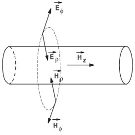
Figure 6: The flux tube filled with the longitudinal magnetic $H^{2}_{z}$ and dressed with color electric $E^{a}_{\rho,\varphi}$ and magnetic $H^{a}_{\rho,\varphi}$ fields.

III Quantum interpretation

In this section we would like to present certain arguments that the derived above dressed flux tube can be considered as a pure quantum object in the SU(3) quantum theory on the nonperturbative level in the first approximation.

One can suppose that in QCD there are two different degrees of freedom vdsin1 , vdsin2 : the first are nonperturbative and the second perturbative degrees of freedom. For us is interesting here only nonperturbative degrees of freedom. In Ref’s vdsin1 , vdsin2 it was supposed that they can be splitted on ordered and disordered phases:

1. The gauge field components $A^{a}_{\mu}\in SU(2),a=1,2,3$ belonging to the small subgroup $SU(2)\subset SU(3)$ are in an ordered phase. It means that

   $$\left\langle A^{a}_{\mu}(x)\right\rangle=(A^{a}_{\mu}(x))_{cl}.$$ (22)

   The subscript means that this is the classical field. It is assumed that in the first approximation these degrees of freedom are classical and is described by appropriate classical equations.

2. The gauge field components $A^{m}_{\mu}$ (m=4,5, … , 8) and $A^{m}_{\mu}\in SU(3)/SU(2)$) belonging to the coset SU(3)/SU(2) are in a disordered phase (or in other words - a condensate), but have non-zero energy. It means that

   $$\left\langle A^{m}_{\mu}(x)\right\rangle=0,\quad\text{but}\quad\left\langle A^{m}_{\mu}(x)A^{n}_{\nu}(x)\right\rangle\neq 0.$$ (23)

   These degrees of freedom are pure quantum degrees and are involved in the equations for the ordered phase as an averaged field distribution of coset components.

In Ref.vdsin2 was made the following assumptions and simplifications:

1. The correlation between coset components $A^{m}_{\mu}(y)$ and $A^{n}_{\nu}(x)$ in two points $x^{\mu}$ and $y^{\mu}$ is

   $$\left\langle A^{m}_{\mu}(y)A^{n}_{\nu}(x)\right\rangle = =-\eta_{\mu\nu}\mathcal{G}^{mn}(y,x)$$ (24)

   $$\mathcal{G}^{mn}(y,x) = -\frac{1}{3}f^{mpb}f^{npc}\phi^{b}(y)\phi^{c}(x)$$ (25)

   where $f^{abc}$ is the structure constants of the SU(3) group.

2. There is not correlation between ordered (classical) and disordered (quantum) phases

   $$\left\langle f(a^{a}_{\mu})g(A^{m}_{\nu})\right\rangle=f(a^{a}_{\mu})\left\langle g(A^{m}_{\mu})\right\rangle$$ (26)

   where $f$ and $g$ are arbitrary functions.

3. The 4-point Green’s function is

   $$\left\langle A^{m}_{\alpha}(x)A^{n}_{\beta}(y)A^{p}_{\mu}(z)A^{q}_{\nu}(u)\right\rangle=\left(E^{mnpq}_{1,abcd}\eta_{\alpha\beta}\eta_{\mu\nu}+E^{mpnq}_{2,abcd}\eta_{\alpha\mu}\eta_{\beta\nu}+E^{mqnp}_{3,abcd}\eta_{\alpha\nu}\eta_{\beta\mu}\right)\phi^{a}(x)\phi^{b}(y)\phi^{c}(z)\phi^{d}(u)$$ (27)

here $E^{mnpq}_{1,abcd},E^{mpnq}_{2,abcd},E^{mqnp}_{3,abcd}$ are constants. The main idea proposed in Ref.vdsin1 is that the initial SU(3) Lagrangian

$$\mathcal{L}_{SU(3)}=-\frac{1}{4}F^{A}_{\mu\nu}F^{A\mu\nu}\;A=1,2,\cdots 8.$$ (28)

after above mentioned assumptions and simplifications can be reduced to the SU(2) Yang - Mills - Higgs Lagrangian

$$\mathcal{L}_{SU(2)}=-\frac{1}{4}F^{a}_{\mu\nu}F^{a\mu\nu}+\frac{1}{2}\left(\partial_{\mu}\phi^{a}-\frac{g}{2}\epsilon^{abc}A^{b}_{\mu}\phi^{c}\right)^{2}+\frac{m^{2}_{\phi}}{2}(\phi^{a}\phi^{a})-\lambda\left(\phi^{a}\phi^{a}\right)^{2}+\frac{g^{2}}{2}a_{\mu}^{b}\phi^{b}a^{c\mu}\phi^{c}.$$ (29)

The first term $F^{a}_{\mu\nu}F^{a\mu\nu}$ is the Lagrangian for the ordered phase $A^{a}_{\mu}$ and the next terms are the Lagrangian for the disordered phase (for the condensate). There is an additional gauge noninvariant term $\frac{g^{2}}{2}a_{\mu}^{b}\phi^{b}a^{c\mu}\phi^{c}$. For the ansätz (3) the corresponding terms in field equations are zero and it is nonimportant for us.

The next remark concerns to the mass $m(a)$. In during of derivation Lagrangian (29) it was assumed that there is a mechanism of generating the mass term $m^{2}_{\phi}\phi^{a}\phi^{a}$ for the disordered phase. By the same way one can suppose that an identical mechanism works for the ordered phase $A^{a}_{\mu}$

$$m^{2}(a)A^{a}_{\mu}A^{a\mu}=m^{2}(1)A^{a}_{\mu}A^{a\mu}+m^{2}(2)A^{a}_{\mu}A^{a\mu}+m^{2}(3)A^{a}_{\mu}A^{a\mu}.$$ (30)

This term will appear in Lagrangian (29) and in field equations (1), additionally we suppose that $m(1)=m(2)=m$ and $m(3)=0$. Therefore we see that above presented dressed flux tube is a pure quantum flux tube in SU(3) quantum theory.

IV Concusions

In this paper we have found the flux tube solution in the SU(2) Yang - Mills - Higgs theory with broken gauge symmetry: it is the Nielsen - Olesen flux tube dressed with the radial and azimuthal color electric and magnetic fields. It was shown that this dressed flux tube can be considered as the tube on the nonperturbative level in quantum SU(3) gauge theory.

It is necessary to note that this tube solution exists only in the presence of gauge symmetry breakdown: $m(1,2)\neq 0$ and $m_{\phi}\neq 0$. It means that there is very close relation between confinement and symmetry breaking phenomena: they are tied in a tight knot. Currently there are different mechanism for generating mass term: the condensation of ghost fields dudal , the Coleman - Weinberg mechanism coleman1 , the nonperturbative symmetry breaking mechanism dzhun . Nevertheless it is not clear how can these mechanisms applicable in the situation presented here. One can say that this problem is not simpler confinement problem and is the task for the future nonperturbative investigations.

Another interesting feature is that the dressed tube exists only by certain values of mass $m$. Probably it is connected with the fact that in full SU(3) quantum theory the mass $m$ will be explicitly calculated that gives us the mass $m$. In our situation the presented here value $m^{2}\approx 0.9402$ is an approximation to a precise value.

We have to note that the presented here the nonperturbative technique strongly differs from perturbative calculations based on Feynman diagrams. Following to Heisenberg heis the nonperturbative calculations in quantum field theory are based on an infinite equations set which connect all Green’s functions. In fact the initial equations (1), (2) are some approximations to this infinite equations set. Our approximation with the ordered and disordered phases allows us to reduce the infinite equations set to the finite field equations (1), (2). The Heisenberg quantization idea is similar to a turbulence theory where all quantities (velocities, pressure and so on) are correlated at different points. These correlators (Green’s functions for quantum field theory) are nor zero for $t=const$ (in contrast to propagators in quantum field theory). By the same way in quantum field theory with strong interactions Green’s functions will be nonzero at one moment $\left\langle Q\left|A^{a}_{\mu}(t,\vec{x})A^{b}_{\mu}(t,\vec{y})\right|Q\right\rangle\neq 0$ in contrast with the case of linear fields where the propagator is zero for one moment. It means that in linear quantum theories (or in theories with weak interactions) the interaction is carried by quanta but in quantum field theory with strong interaction (like to turbulence) can exist a field distributions where the field magnitudes at the different points and at one moment are correlated.

V Acknowledgments

I am very grateful to the ISTC grant KR-677 for the financial support.

References

• (1) H.B. Nielsen and P. Olesen, Nucl. Phys. B61, 45 (1973).
• (2) M.Β A.Β Kneipp and P.Β Brockill, Phys.Β Rev.Β D64, 125012(2001); M.Β A.Β Kneipp, hep-th/0211146; M.Β A.Β Kneipp, hep-th/0211049.
• (3) V. Dzhunushaliev and D. Singleton, Phys. Rev., D65, 125007 (2002).
• (4) V. Dzhunushaliev and D. Singleton, β€œGinzburg - Landau equation from SU(2) gauge field theory”, Mod. Phys. Lett., A18, 955(2003), hep-th/0210287; V. Dzhunushaliev and D. Singleton, β€œEffective ’t Hooft-Polyakov monopoles from pure SU(3) gauge theory”, hep-ph/0306202.
• (5) Y.Β N.Β Obukhov, Int.Β J.Β Theor.Β Phys.Β  37, 1455 (1998).
• (6) D. Dudal and H. Verschelde, β€œOn ghost condensation and Abelian dominance in the Maximal Abelian Gauge”, hep-th/ 0209025; V.E.R. Lemes, M.S. Sarandy, and S.P. Sorella, β€œGhost number dynamical symemtry breaking in Yang-Mills theories in the maximal Abelian gauge”, hep-th/0206251.
• (7) S. Coleman and E. Weinberg, Phys. Rev. D7, 1888 (1973).
• (8) V. Dzhunushaliev, β€œNonperturbative spontaneous symmetry breaking”, Found. Phys. Lett., 16, 265(2003), hep-th/0208088.
• (9) W. Heisenberg, Introduction to the unified field theory of elementary particles., Max - Planck - Institut fΓΌr Physik und Astrophysik, Interscience Publishers London, New York, Sydney, 1966; W. Heisenberg, Nachr. Akad. Wiss. GΓΆttingen, N8, 111(1953); W. Heisenberg, Zs. Naturforsch., 9a, 292(1954); W. Heisenberg, F. Kortel und H. MΓΌtter, Zs. Naturforsch., 10a, 425(1955); W. Heisenberg, Zs. fΓΌr Phys., 144, 1(1956); P. Askali and W. Heisenberg, Zs. Naturforsch., 12a, 177(1957); W. Heisenberg, Nucl. Phys., 4, 532(1957); W. Heisenberg, Rev. Mod. Phys., 29, 269(1957).