CHAOTIZATION OF THE PERIODICALLY DRIVEN QUARKONIA

Abstract

Classical regular and chaotic dynamics of the particle bound in the Coulomb plus linear potential under the influence of time-periodical perturbations is treated using resonace analysis. Critical value of the external field at which chaotization will occur is evaluated analytically based on the Chirikov criterion of stochasticity.

1 Introduction

Theory of dynamical chaos is one the rapidly developing fields of the contemporary physics. It has found applications not only in various areas of physics but also in many other areas natural sciences. Therefore the deterministic, or dynamical chaos is becoming the subject of extensive theoretical as well as experimental investigation now chir -del83 .

Dynamical chaos is a phenomenon peculiar to the dynamical (deterministic) systems, whose motion in some state space is completely determined by a given interaction and the initial conditions. However, under appropriate conditions, the behavior of these systems are indistguishible from random behavior despite the absence of noise or thermal fluctuations. Among the theoretical models used to study and illustrate chaotic behavior are various confined billiards geometries eckh88 , nonlinear oscillatorschir ; esca85 ; eckh88 , highly excited atoms in mono- and poly-chromatic fields jens ; koch ; del83 , kicked rotatorIzr90 , and a number of astrophysical systemszas88 . In recent years a wide variety of experimental systems have emerged in which simple theoretical paradigms have been realized and which provide controlled environments to test and apply ideas. One of the main features of dynamical chaos is the strong sensitivity of the evolution of the dynamical system with respect to changes in the initial conditions. The small changes in the initial conditions may lead to considerable changes in the evolution. As is well known chir ; eckh88 ; Zas ; jens84 chaotic motion occurs when the phase-space trajectories corresponding to neighboring resonances overlap each other. This fact gives a criterion for the estimates of stochasticity. One of the commonly used criterions of stochasticity, Chirikov criterion, is based on this fact.

Dynamical systems which can exhibit chaotic dynamics can be divided into two classes: time independent and time-dependent systems. Billiards, atoms in a constant magnetic field, celestial systems with chaotic dynamics are time independent systems, whose dynamics can be chaotic. Periodically driven rotators and pendula, atoms and molecules in a microwave field, and many other periodicallyy driven dynamical systems are time-dependent systems, whose dynamics can be chaotic. A convenient testing ground for the theoretical and experimental study of chaos in the time-dependent dynamical systems is the highly excited hydrogen atom in a monochromatic field cas87 ; jens ; koch ; del83 . A theoretical analysis, of the behaviour of a classical hydrogen atom interacting with monochromatic field, based on the resonance overlap criterion del83 -mat1 , shows that for some critical value of the external field strength $\epsilon_{cr}$, the electron enters into chaotic regime of motion, marked by unlimited diffusion along orbits, leading to ionization. Experimentally this phenomenon was first observed by Bayfield and Koch bay74 . Theoretical explanation of this phenomenon was given later by severeal authors del ; del83 ; koch . Such an ionization was called chaotic cas87 ; jens or diffusive del83 ionization. During the last three decades chaotic ionization of nonrelativistic atom was investigated by many authors theoretically jens84 ; del83 ; cas87 ; cas88 ; del as well as experimentally jens ; bay74 ; koch .

In this paper we consider the QCD counterpart of this problem. Namely, we address the problem of regular and chaotic motion in periodically driven quarkonium. Using resonanse analysis based on the Chirikov criterion of stochasticity we estimate critical values of the external field strength at which quarkonium motion enters into chaotic regime.

Quarkonium in a monochromatic field can be considered as an analog of the hydrogen atom in a monochromatic field, in which Coulomb potential is replaced by Coulomb plus confining potential. Quarkonia have been the subject of extensive experimental as well as theoretical studies for the last two decades AL -Zhu . In the framework of potential approach the description of quark motion in hadrons is reduced to solving classical or quantum mechanical equations of motion with Coulomb plus confining potential. Considerable progress has been made in the calculation of the spectra of quarkonium Quig -Zhu . At present a large amount of theoretical and experimental data on quarkonium properties is available. Due to the presence of the confining potential quarkonium motion is equivalent to the atom in an uniform magnetic field whose dynamics is also chaotic eckh88 ; Wint . Recently chaotic dynamics in hadrons and QCD has become a subject of theoretical studies Gu -Buk . In particular, it is found that QCD is governed by quantum chaos in both confined and deconfined phases Hal ; Bit . The statistical analysis of the measured meson and baryon spectra shows that there is quantum chaos phenomenon in these systems Pasc . The study of the charmonium spectral statistics and its dependence on color screening has established quantum chaotic behaviour Gu . It was claimed that such a behaviour could be the reason for $J/\Psi$ supression Gu . Study of the chaotic dynamics of the periodically driven quarkonium is needed due to the recent advances in the creation of hot and dense matter, such as hadronic matter and quark-gluon plasma. Being in a quark gluon plasma or in hadronic matter quarkonium can be subjected to the influence of time-dependent fields, that can lead to chaotization of the quarkonium and level fluctuations. Indeed, the study of the spectral statistics of the charmonium based on the solution of the Bethe-Salpether equation for the potential with color screening shows that regular motion can be expected at a small values of color screening mass but the chaotic motion is expected at a large one Gu . Periodically driven quarkonium can be also realized in the interaction of mesons with laser fields. It should be noted, that being a confined system quarkonium can exhibit chaotic motion even in the absence of any exterenal force. It is well known that many realistic and model confined dynamical systems as an atom in a magnetic fieldWint , particle motion in resonators ding , quantum dotsalh and various billiards Zas can exhibit chaotic dynamics. In next section we will treat a simple model, a one-dimensional quarkonium under a periodic perturbation. In section 3 we extend our treatment to the three-dimensional case. Some concluding remarks are given in section 4.

2 One-dimensional model

For simplicity we consider a one-dimensional model with a potential

$$V(x)=\left\{\begin{array}[]{ll}-\frac{Z}{x}+\lambda x&for\;\>x>0\\ \\ \infty&for\>\;x\leq 0\end{array}\right.\,,$$

where $Z=\frac{4}{3}\alpha_{s}$ $\alpha_{s}$ being the strong coupling constant and $\lambda$ gives strength of the confining potential. As is well known, in the case of the hydrogen atom interacting with a monochromatic field, one-dimensional model provides an excellent description of the experimental chaotization thresholds for real three-dimensional hydrogen atom jens ; jens84 ; cas87 . The same success is to be expected in the case of quarkonium.

The unperturbed Hamiltonian for the above potential is

$$H_{0}=\frac{p^{2}}{2}-\frac{Z}{x}+\lambda x.$$ (1)

We will treat the interaction of the system given by Hamiltonian (1) with the periodic external potential of the form

$$U(x,t)=\epsilon xcos\omega t.$$ (2)

with $\epsilon$ and $\omega$ being the field strength and frequency, respectively. Thus the total Hamiltonian of the periodically driven quarkonium is

$$H=H_{0}+U(x,t)$$ (3)

Formally the Hamiltonian (1) is equivalent to the Hamiltonian of the hydropen atom in constant homogenious electric field. Chaotic dynamics of hydrogen atom in constant electric field under the influence of time-periodic field was treated earlier ber ; bala . To treat nonlinear dynamics of this system under the influence of periodic perturbations we need to rewrite (1) in action-angle variables. Action can be found using its standard definition:

$$n(E)=\frac{1}{2\pi}\int\limits_{c}^{a}pdx=\sqrt{2\lambda}\int\limits_{c}^{a}\sqrt{\frac{(a-x)(x-c)}{x}}dx,$$ (4)

where the momentum $p$ is given by

$$p=\sqrt{2(E-V(x))},$$ (5)

and the constants $a$ and $c$ given as

$$a=\frac{E+\sqrt{E^{2}+2Z\lambda}}{2\lambda},\;\;\;c=\frac{E-\sqrt{E^{2}+2Z\lambda}}{2\lambda}$$

are turning points of the particle. Since $c<0$ for the action we have

$$n(E)=\frac{1}{2\pi}\int\limits_{0}^{a}pdx=$$

$$=B\sqrt{a+\frac{1}{a}}\cdot\Biggl{[}\biggl{(}a-\frac{1}{a}\biggr{)}E(k)+\frac{1}{a}K(k)\Biggr{]}.$$ (6)

where

$$B=\frac{2\sqrt{2}}{3\pi\lambda^{\frac{1}{4}}},$$

here $E(k)$ and $E(k)$ are the elliptic integralsabr and

$$k^{2}=\frac{a^{2}}{a^{2}+1}-(1+\frac{1}{a^{2}})^{-1}.$$ (7)

Here we consider the two limit cases: $a\gg 1$ and $a\ll 1$.

For the first case ($a\gg 1$) we have:

$$E\equiv H_{0}=Z^{2}An^{2/3}\cdot\Biggl{[}1-\frac{\lambda ln4B^{-2/3}n^{2/3}}{A^{2}n^{4/3}}\Biggr{]},$$ (8)

with

$$A=\biggr{(}\frac{3\pi\lambda}{2\sqrt{2}}^{\frac{2}{3}}\biggl{)}.$$

The corresponding proper frequency is

$$\omega_{0}=\frac{2}{3}Z^{2}\biggr{[}\frac{A}{n^{1/3}}+\frac{\lambda}{An^{5/3}}\bigr{[}\ln(4A\sqrt{\lambda}n^{2/3})\bigl{]}-1\biggl{]}$$ (9)

For the case $a\ll 1$ we have:

$$E\equiv H_{0}=0.5Z^{2}(9.7\lambda n^{2}-n^{-2});$$ (10)

The proper frequency for this Hamiltonian is

$$\omega_{0}=Z^{2}(n^{-3}+9.7n\lambda).$$ (11)

The total Hamiltonian can be written as

$$H=H_{0}+\epsilon\sum x_{k}cos(k\theta-\omega t),$$ (12)

with

$$x_{k}(n)=-\int_{0}^{2\pi}x(n,\theta)e^{ik\theta}d\theta$$ (13)

being Fourier amplitude of the perturbation. For $a\ll 1$ we have an estimate for the Fourier component

$$x_{k}(n)\approx-\frac{4E(n)}{\lambda}\frac{1}{k}\sin^{2}\frac{\pi k\sqrt{\lambda}}{2}.$$ (14)

For $a\gg 1$ we have

$$x_{k}(n)=-\frac{2An^{2/3}}{\pi^{2}\lambda k^{2}}.$$ (15)

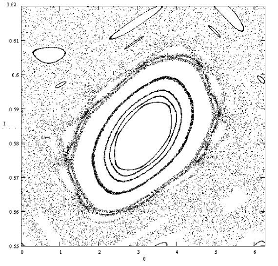
Figure 1: Phase space portrait of the periodically driven quarkonium: $a>>1$ case.

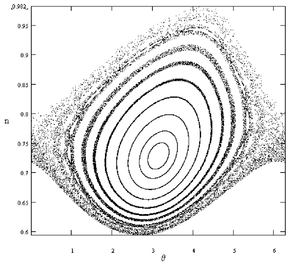
Figure 2: Phase space portrait of the unperturbed quarkonium: $a<<1$ case.

It is well known that the phase-space trajectories of the regular motion lie on tori(so-called KAM tori). According to Kolmogorov-Arnold-Moser theorem for sufficiently small fields most of the trajectories remain regular. If the value of the external perturbation exceeds some value, which is called the critical field strength, KAM tori start to break down and chaotization of the motion will occur zas88 . In Fig. 1 the phase-space portrait of the periodically driven quarkonium is plotted for the following values of parameters: $Z=0.15$, $\lambda=0.4$, $\omega=10^{-5}$ and $\epsilon=4\cdot 10^{-4}$. Eight regular and two chaotic trajectories are shown. The values of these parameters are written in the systems of units where $m_{q}=\bar{h}=1$, where $m_{q}$ is quark mass, $c$ is the light speed. The values are chosen to have chaotic as well as regular behaviour. Fig.2 represents the pahse-space portrait of the periodically driven quarkonium for $a\ll 1$ case for the values of parameters $Z=0.15$, $\lambda=10$, $\omega=10^{-5}$ and $\epsilon=4\cdot 10^{-3}$. Again, the system of units $m_{q}=\bar{h}=1$ is used.

To estimate the critical value of the external filed strength $\epsilon_{cr}$ we use Chirkov’s resonance overlap criterion chir ; zas88 ; del83 ; jens ; koch , which can be written as:

$$s=\frac{\Delta\nu_{k}+\Delta\nu_{k+1}}{\omega_{0}(k+1)-\omega_{0}(k)},$$ (16)

with

$$\Delta\nu_{k}=(\frac{\epsilon x_{k}}{\omega_{0}^{\prime}})$$

being the width of the $k$-th resonance chir ; zas88 and

$$\omega_{0}^{\prime}=d\omega_{0}/dn.$$

From the resonance condition we have

$${\omega_{0}(k)-\omega_{0}(k+1)}=\frac{\omega}{k}-\frac{\omega}{k+1}=\frac{\omega}{k(k+1)}.$$

Applying this criterion to the quarkonium Hamiltonian (12) we have for $a\gg 1$

$$\epsilon_{cr}=\frac{0.07Z^{2}\omega\pi^{2}\lambda}{n^{2}}\cdot\frac{k(k+1)}{(k+1)^{2}+k^{2}}\times$$

$$\left\{1+\frac{\lambda}{A^{2}n^{\frac{4}{3}}}\left[5\ln\left(4A\lambda^{-\frac{1}{2}}n^{\frac{2}{3}}\right)-7\right]\right\}$$ (17)

and for $a\ll 1$:

$$\epsilon_{cr}=\frac{0.3\omega\alpha}{k(k+1)n^{2}}\cdot\frac{29\alpha n^{4}-9}{29\alpha n^{4}-3}\times$$

$$\times\left[\frac{1}{k}\sin^{2}(k\sqrt{\alpha}\frac{\pi}{2})+\frac{1}{k+1}\sin^{2}((k+1)\sqrt{\alpha}\frac{\pi}{2})\right]^{-1}$$ (18)

In Table 1 the values of the critical field for both approximations for $u\bar{u}$, $d\bar{d}$, $s\bar{s}$, $c\bar{c}$ and $b\bar{b}$ quarkonia at the following values of parameters: $\omega=10^{9}Hz$, $\alpha_{s}=0.112$PDG , $\lambda=0.2Gev^{2}$, $n=10$. are presented. For light ($u,d,s$) quarkonia we use formula (17) and formula (18) for bottomium and charmonium.

3 Three-dimensional model

The Hamiltonian for the three-dimensional model is

$$H_{0}=\frac{p^{2}_{r}}{2}-\frac{Z}{r}+\lambda r+\frac{L^{2}}{r^{2}}.$$

where $L$ is the orbital angular momentum and $p_{r}$ is the radial momentum.

The action can be expressed in terms of elliptic integrals seet :

$$n=\int\limits_{c}^{a}pdr=\int\limits_{c}^{a}\sqrt{2(E-\frac{L^{2}}{r^{2}}+\frac{Z}{r}-\lambda r)}dr=$$

$$\left[(2Z/3-L^{2}/c+Ec/3)K(k)+E(a-c)/3E(k)+\right.$$

$$\left.+L^{2}(c^{-1}-b^{-1})\prod(\beta^{2},k)\right]g/\sqrt{\lambda}$$ (19)

with $a$ and $c$ being the turning points, $K,E,\prod$ are complete elliptic integrals of the first, second and third kind, respectively abr , and the constants are given as

$$k^{2}=(a-b)/(a-c),$$

$$\beta=ck^{2}/b,$$

$$g=2/\sqrt{a-c}.$$

From eq.(19) the unperturbed Hamiltonian as a function of $n$ can be found approximately for $E/\lambda\gg 1$, (which corresponds to $n\gg 1$ or large quarkonium masses):

$$H_{0}=(\frac{3}{2}\lambda n)^{2/3}\left[1+\frac{\pi L}{3n}\right].$$

The proper frequency is

$$\omega_{0}=\frac{\partial H_{0}}{\partial n}=(\frac{2\lambda^{2}}{3})^{1/3}.\left[n^{-1/3}-\frac{\pi L}{6}n^{-4/3}\right]$$

Then the Hamiltonian of the three-dimensional quarkonium in a monochroamtic field can be written as

$$H=H_{0}+\epsilon a\cos(\omega t)\times$$

$$\{-\frac{3}{2}e\sin\varphi+2\sum[x_{k}\sin\psi\cos k\phi+y_{k}\cos\psi\sin k\phi]\},$$ (20)

where

$$x_{k}=\frac{2i}{\omega_{0}kT}\int e^{i\omega_{0}kt}\dot{x}dt,\;\;\;\;y_{k}=\frac{2i}{\omega_{0}kT}\int e^{i\omega_{0}kt}\dot{y}dt,$$

and $\psi$ and $\phi$ are the Euler angles. Again, using the resonance overlap criterion (16) in which the resonance width is defined by

$$\Delta\nu_{k}=(\frac{\epsilon r_{k}}{\omega_{0}^{\prime}}),$$

where

$$r_{k}=\sqrt{x_{k}^{2}+y_{k}^{2}},$$

we obtain an estimate for the critical field:

$$\epsilon_{cr}=\frac{0.07\alpha\omega}{k(k+1)\pi n^{2}}\left(1-\frac{\pi L}{n}\right)$$

$$\left\{\sqrt{\frac{16\pi^{2}}{9}+\frac{1}{k^{2}}}+\sqrt{\frac{16\pi^{2}}{9}+\frac{1}{(k+1)^{2}}}\right\}^{-1}$$

$$\times\left[1-\frac{L^{2}}{4\pi^{4}n^{2}}\right].$$ (21)

This estimate for the critical field assumes that $n$ is large. If the external field strength has the value exceeding $\epsilon_{cr}$, breaking of KAM surfaces in the pase space will occur and and the quarkonium diffuses in action and the motion becomes chaotic.

4 Conclusions

Summarizing we have treated the chaotic dynamics of the quarkonium in a time periodic field. Using the Chirikov’s resonance overlap criterion we obtain estimates for the critical value of the external field strength at which chaotization of the quarkonium motion will occur. The experimental realization of the quarkonium motion under time periodic perturbation could be performed in several cases: in laser driven mesons and in quarkonia in the hadronic or quark-gluon matter. The quarkonium, being the QCD analog of the hydrogen atom can be also considered as a confined atom. However, as is seen from the above treatment, in contrast to the case of periodically driven atom, where the absolute value of the energy decreases diffusively, the energy of the quarkonium in a monochromatic field grows by diffusive law.

5 Acknowledgements

The work of DUM is supported by NATO Science Fellowship of Natural Science and Engineering Research Council of Canada (NSERCC). The work of FCK is supported by NSERCC. The work of DMO is supported by a Grant of the Uzbek Academy of Sciences (contract No 33-02).

References

- (1) B.V.Chirikov Phys.Rep., 52, 159, (1979)
- (2) D.F. Escande, Phys. Rep. 121, 167, (1985)
- (3) G.Casati, et al., Phys.Rep. 154 77 (1987)
- (4) B. Eckhardt, Phys. Rep. 163, 207, (1988)
- (5) R.Z.Sagdeev, D.A.Usikov, G.M.Zaslavsky, Nonlinear Physics: from pendulum to turbulence and chaos (Academic Publisher, NY 1988)
- (6) G.M.Izrailev, Phys.Rep., 196 299 (1990)
- (7) R.V.Jensen , S.M.Susskind and M.M.Sanders Phys.Rep. 201, 1 (1991)
- (8) P.M.Koch, K.A.H. van Leeuwen Phys.Rep. 255 (1998) 289
- (9) N.B.Delone, V.P.Krainov and D.L.Shepelyansky, Usp. Fiz. Nauk. 140, 335, (1983)
- (10) R.V.Jensen, Phys.Rev. A, 30, 386, (1984)
- (11) G.M.Zaslavsky, Stochastic Behaviour of Dynamical Systems. New York, Harwood. 1985. IEEE J.Quant.Electronics. 24, 1420 (1988).
- (12) G.Casati, B.V.Chirikov and D.L.Shepelyansky, Phys.Rep., 154, 77, (1987)
-
(13)
G.Casati, I.Guarneri and D.L.Shepelyansky
- (14) N.B.Delone, B.A.Zon and V.P.Krainov JETP, 75 445 (1978)
- (15) D.U.Matrasulov, Phys.Rev. A 50 700 (1999)
- (16) J.E.Bayfield and P.M.Koch, Phys.Rev.Lett., 33, 258, (1974)
- (17) ALEPH Collaboration, R.Barate, et al., Phys.Lett. B, 425 215 (1998).
- (18) C.Quigg and J.L.Rosner , Phys.Rep., 56 167 (1979).
- (19) W.Lucha, F.F.Schoberl and D.Gromes, Phys.Rep., 200 128 (1991).
- (20) S.N.Mukherjee et.al. Phys.Rep. 231 (1993) 203
- (21) V.A.Novikov et.al. Phys.Rep. 41 (1978) 1
- (22) H.Friedrich and D.Wintgen, Phys.Rep., 183 38 (1989).
- (23) X.Q.Zhu, F.C.Khanna, R.Gurishankar and R.Teshima, Phys.Rev.D, 47 1155 (1993).
- (24) Jian-zhong Gu et al, Phys.Rev.C, 60 035211 (1999).
- (25) M.A.Halasz and J.J.M.Verbaarschot, Phys.Rev. Lett., 74 3920 (1995).
- (26) E.Bittner, Harald Markum and Reiner Pullrich Quantum chaos in physical systems: from super conductors to quarks. hep-lat/0110222.
- (27) Vladimir Pascalusta, hep-ph/0201040.
- (28) B.A.Berg, et.al hep-lat/0007008.
- (29) D. Bukta, G. Karl, B. G. Nickel chao-dyn/9910026.
- (30) J. Dingjan, E. Altewischer, M. P. van Exter, and J. P. Woerdman Phys. Rev. Lett. 88, 064101 (2002)
- (31) Y.Alhassid, Rev.Mod. Phys., 72 895 (2000)
- (32) G. P. Berman, G. M. Zaslavskii, and A. R. Kolovskii, Sov. Phys. JETP, 61 925 (1985)
- (33) Mark J. Stevens and Bala Sundaram, Phys.Rev. A, 36, 417, (1987)
- (34) M.A. Abramowitz and I.A. Stegun, Handbook of mathematical functions, Nat. Bur. Stand. Washington D.C.,1964;
- (35) Particle Data Group, R.M.Barnett et al Phys.Rev.D, 54 1 (1996)
- (36) M.Seetharaman, R.Raghavan and S.S.Vasan J.Phys.A 16 455(1983)
Table 1. The values of the critical field strength for various quarkonia.