SISSA 54/2003/EP hep-ph/0306195

Charged Lepton Flavor Violating Decays:
Leading Logarithmic Approximation
versus Full RG Results

S. T. Petcov ^a,b),  S. Profumo ^a,b),  Y. Takanishi ^c),  C. E. Yaguna ^a)

^a)Scuola Internazionale Superiore di Studi Avanzati, I-34014 Trieste, Italy ^b)Istituto Nazionale di Fisica Nucleare, Sezione di Trieste, I-34014 Trieste, Italy ^c)The Abdus Salam International Centre for Theoretical Physics, Strada Costiera 11, I-34100 Trieste, Italy

In the context of the minimal supersymmetric extension of the Standard Model with the right-handed Majorana neutrinos, we study lepton flavor violating processes including full renormalization group running effects. We systematically compare our results with the commonly used leading logarithmic approximation, resorting to a “best fit” approach to fix all the high energy Yukawa matrices. We find significant deviations in large regions of the SUSY parameter space, which we outline in detail. We also give, within this setting, some results on the cosmo-phenomenologically preferred stau coannihilation region. Finally, we propose a parametrization, in terms of the SUSY input parameters, of the common SUSY mass appearing in the leading log and mass insertion approximation formula for the charged lepton flavor violating decay rates, which fits our full renormalization group results with high precision.
 PACS numbers: 11.10.Hi, 12.60.Jv, 14.60.St.
 Keywords: Lepton Flavor Violating Processes, Supersymmetric Models, Neutrino Physics.

June 2003

1 Introduction

In the Standard Model (SM) with left-handed massive neutrinos, lepton flavor violating (LFV) processes, such as the muon decay into electron and photon, $\mu\to e\gamma$, or tau decay into muon and photon, $\tau\to\mu\gamma$, are extremely suppressed: the branching ratios for these processes are typically less than $10^{-54}$ [1], henceforth far beyond experimental reach. However, this situation changes drastically if the SM is embedded in its (minimal) supersymmetric extension, including heavy right-handed neutrinos, responsible for the generation of low energy neutrino masses via the see-saw mechanism (MSSMRN) [2, 3].

The compelling evidences for neutrino mixing, coming from solar and atmospheric neutrino, and KamLAND experiments [4], indicate that the lepton charges are not conserved quantities: as a consequence, it is not possible to choose a flavor and gauge interaction diagonal basis in the lepton sector (see, e.g., [5]).

The off-diagonal elements of the supersymmetry soft-breaking (SSB) terms in the slepton mass matrices, $\left(m_{\widetilde{\scriptscriptstyle L}}^{2}\right)_{ij}$, $\left(m_{\widetilde{e}}^{2}\right)_{ij}$, and trilinear scalar couplings, $\left(A_{e}\right)_{ij}$ ($i\not=j$) represent new direct sources of lepton flavor (charge) violation which are not suppressed by the extremely small light neutrino masses. The resulting LFV decay branching ratios, though highly dependent on the structure of the theory (e.g., the right-handed neutrino masses, neutrino Yukawa couplings, slepton soft SUSY breaking terms etc.) are typically in the range of sensitivity of the current and planned experiments searching for such decays.

A critical issue in the study of the predictions for the LFV decay rates in the SUSY theories incorporating the see-saw mechanism of neutrino mass generations is the relation between the high energy input parameters and the low energy phenomena. This relation is mainly dictated by radiative corrections encompassed in the renormalization group (RG) equations.

A common approach to RG evolution in the context of LFV is to resort to the simple leading logarithmic approximation. In [3] it has been shown that, in the specific case of sequential dominance in the neutrino Yukawa couplings, the leading log approximation may lead to an underevaluation of the off-diagonal entries of the slepton mass matrix. The aim of the present work is to show in a general setting what are the effects of taking into account the full RG running and to provide evidence of what is the parameter space where the leading log approximation ceases to give a reasonable approximation to the full result. We do not make any particular assumption about the neutrino Yukawa coupling matrix, but instead we resort to a best fit procedure, which allows us to sit on a (particular) viable solution, compatible with the known parameters of the neutrino sector. We also calculate, within this RG approach, the absolute value of some LFV decay rates in a cosmologically and phenomenologically allowed parameter space region of a minimal supergravity (mSUGRA) MSSM, namely, the one where neutralino-stau coannihilation processes take place. Finally, we present an effective parametrization of the common SUSY mass $m_{\scriptscriptstyle S}$ appearing in the commonly used approximate formula for the $l_{j}\rightarrow l_{i}\gamma~{}(m_{l_{j}}>m_{l_{i}})$ decay branching ration, $l_{3}\equiv\tau$, $l_{2}\equiv\mu$, $l_{1}\equiv e$, in terms of the high energy input parameters of mSUGRA, the universal gaugino mass $M_{1/2}$ and the common SSB scalar mass $m_{0}$, both taken at the GUT scale. We demonstrate that our parametrization allows to reproduce with high precision the exact RG result in a large region of relevant parameter space.

The paper is organized as follows: in the next Section, we discuss the current phenomenological constraints on the SUSY parameter space, on neutrino masses and mixings and on LFV processes. In Section 3 we illustrate our numerical approach and methodology, while in Section 4 we discuss the relevant RG equations. Our results are presented in Section 5. Finally, Section 6 is devoted to conclusions. Details regarding the formalism used for the calculations performed in the present study are given in Appendices A and B.

2 Phenomenological Setting

The main ingredients entailing non negligible rates for LFV processes in the context of the MSSMRN are (1) the structure of the SSB terms and (2) the neutrino mixing in the lepton sector of the theory. We devote this section to the discussion of the SUSY breaking sector (Sec. 2.1), which is currently restricted by both cosmological and accelerator data [6], and the problem of determination of the high energy structure of the Yukawa couplings of the theory (Sec. 2.2). It is well known that low energy data allow to reconstruct only partially the high energy couplings of the theory. Finally, we will briefly discuss how LFV processes arise in the context of MSSMRN theories (Sec. 2.3).

2.1 SUSY Parameter Space

In the MSSM, the Standard Model fields are promoted to superfields and the theory is defined by a superpotential $W$ and by a soft SUSY breaking Lagrangian $\mathscr{L}_{\rm soft}$. This last part results after a formal integration over the hidden sector fields which break SUSY. In its most general setup, $\mathscr{L}_{\rm soft}$ depends a priori on more than one hundred parameters, which are, however, constrained both by theoretical arguments (e.g., naturalness in the Higgs sector) and experimental data (e.g., absence of flavor changing neutral currents). The specific form of $\mathscr{L}_{\rm\scriptscriptstyle SSB}$ relies on the mechanism which communicates SUSY breaking from the hidden to the visible sector. If one resorts to non-trivial assumptions about high energy physics, such as Grand Unification or specific supergravity Kähler potentials, a further reduction of the number of parameters can occur. One of the most common settings is the so-called minimal supergravity (mSUGRA) [7]. The auxiliary chiral field giving mass to the gauginos is supposed to lie, in mSUGRA, in the trivial representation of the symmetric product of two adjoints of the GUT gauge symmetry group, hence generating a universal gaugino mass, $M_{1/2}$. Moreover, the scalar soft breaking part of the Lagrangian depends only on a common scalar mass $m_{0}$ and trilinear coupling $A_{0}$, as well as on $\tan\beta$. Fixing an extra sign-ambiguity in the Higgs mass term $\mu$ completes the parameter space of mSUGRA, which then reads

$$M_{1/2},\ m_{0},\ A_{0},\ \tan\beta,\ {\rm sign}(\mu)\hskip 5.69054pt.$$ (1)

These parameters are restricted by accelerator and cosmological constraints. An obvious accelerator constraint comes from negative searches for superpartners at LEP2 [8]. In mSUGRA models, however, the most stringent bounds come from indirect phenomenological implications of SUSY. For instance, the limits on the almost SM like lightest $CP$-even neutral Higgs boson put a strong constraint at $m_{h}>114.1~{}\mbox{\rm GeV}$, which, being $m_{h}(m_{\chi})$ an increasing function of its arguments, translates into a lower bound on $m_{\chi}$ [9]. Analogously, the inclusive branching ratio ${\rm BR}(b\rightarrow s\gamma)$ [10] receives SUSY contributions proportional to $\tan\beta$ and inversely proportional to $m_{\chi}$. The current experimental data [11], combined with the SM theoretical uncertainties, give the overall bound [12]

$$2.16\times 10^{-4}<{\rm BR}(b\rightarrow s\gamma)<4.34\times 10^{-4}\hskip 5.69054pt.$$ (2)

The bound of Eq. (2) translates into a lower bound for the mass of the LSP. We also mention the constraint coming from the deviation $\delta a_{\mu}$ of the measured muon anomalous magnetic moment from its SM value [13]. In this case the current theoretical uncertainties in the SM computations, mainly due to the evaluation of the hadronic vacuum polarization contribution, make it difficult to draw a bound from this quantity. Therefore, this bound is not taken as a constraint in the present work.

Since supersymmetric models with conserved $R$-parity offer a natural (i.e. stable, massive and weakly interacting) candidate for the non-baryonic matter content of the Universe (Dark matter), namely the lightest neutralino $\chi$, it is natural to require that the relic density fraction $\Omega_{\chi}$ of neutralinos falls into the cosmologically preferred range. In this respect, the recent data from WMAP [14] greatly increased the accuracy of previous determination of the Dark Matter content of the Universe, indicating that

$$\Omega_{\rm\scriptscriptstyle CDM}\ h^{2}\ =\ 0.1126^{+0.0081}_{-0.0091}\hskip 5.69054pt.$$ (3)

As the lower limit can be evaded under the hypothesis of the existence of another cold dark matter component besides neutralinos, we take here as a constraint only the upper bound $\Omega_{\chi}h^{2}\lesssim 0.13$. Imposing on the mSUGRA parameter space (1) the constraints coming both from cosmology and from accelerator experiments typically reduces the viable values of the parameters $m_{0}$ and $M_{1/2}$ to very narrow strips [15].

The major problem, in the framework of mSUGRA, is that the annihilations of bino-like neutralinos is generally not sufficiently efficient, and the resulting $\Omega_{\chi}$ exceeds the previously stated upper bound. Specific relic density suppression mechanisms are needed in order to achieve reasonable values for $\Omega_{\chi}$. Exhaustive investigations of the mSUGRA parameter space showed that only four regions of the parameter space are compatible with Eq. (3) [12]. $(1)$ A bulk region where the neutralino is sufficiently light and no specific suppression mechanism is needed; this region is, however, severely restricted by increasingly accurate accelerator bounds. $(2)$ A coannihilation region, where the lightest supersymmetric particle (LSP) is quasi degenerate with the next-to-LSP (NLSP). In this case, the freeze out of the two species occurs at close cosmic temperatures, and co-annihilations between the NLSP and the LSP can drastically reduce the relic density of the latter. $(3)$ A focus region, at high $m_{0}$, close to the region excluded by the absence of radiative electroweak symmetry breaking, where the LSP gets a non negligible fraction of Higgsino, thus enhancing direct annihilation into gauge bosons. $(4)$ A funnel region, where $2m_{\chi}\simeq m_{A}$, $m_{A}$ being the mass of the $CP$-odd neutral Higgs boson of the MSSM. In this region, which opens only at large $\tan\beta$, resonance effects suppress the relic density through direct $s$-channel pole annihilations.

In this paper we will only exploit the coannihilation region, since the coannihilation mechanism can occur at every $\tan\beta$, and also takes place in a relatively “stable” SUSY parameter space region, contrary to the “focus” and “funnel” regions. Moreover, it has been recently shown [16] that in supergravity models where some relation exists between the trilinear and bilinear soft supersymmetry breaking parameters $A_{0}$ and $B_{0}$ (e.g., the Polonyi model or particular no-scale models) only the coannihilation region survives after the cosmological and phenomenological constraints are applied.

In general, at a fixed value of $\tan\beta$, the stau coannihilation strip lies at values of $m_{0}\simeq aM_{1/2}+b$. The minimum $M_{1/2}$ value reflects the lower bound on $m_{\chi}$, dictated by accelerator constraints, while the maximal $M_{1/2}$ value is given by the saturation of the bound (3) at $m_{\chi}\simeq m_{\scriptscriptstyle\rm NLSP}$.

2.2 Neutrino Sector

The right-handed neutrino Majorana mass term, $M_{R}$, and the neutrino Yukawa couplings, $Y_{\nu}$, produce an effective Majorana mass matrix (see Sec. 4) for the left-handed neutrinos. This is the well-known see-saw mechanism [17]:

$$M_{\rm eff}\!\! \simeq \!\!M_{\nu}^{\sf T}\,M_{R}^{-1}\,M_{\nu}$$ (4)

$$\simeq \!\!v_{u}^{2}\sin^{2}\beta\>Y_{\nu}^{\sf T}M_{R}^{-1}Y_{\nu}\hskip 5.69054pt,$$

where $v_{u}$ is vacuum expectation value (VEV) of up-type Higgs field, $v_{u}=246/\sqrt{2}~{}\mbox{\rm GeV}$. In what follows we do not consider contributions other than that in Eq. (4) to the left-handed Majorana mass term.

The matrix $M_{\rm eff}$ is diagonalized by a single unitary matrix according to

$$M_{\rm eff}^{\mathrm{diag}}=U^{\sf T}_{\rm eff}M_{\rm eff}U_{\rm eff}=\mathrm{diag}\left(m_{1},m_{2},m_{3}\right)\hskip 5.69054pt.$$ (5)

Let us define by $U_{e}$ the unitary matrix which diagonalizes $M_{e}^{\dagger}M_{e}$, where $M_{e}$ is the charged lepton mass matrix,

$$U_{e}^{\dagger}M_{e}^{\dagger}M_{e}U_{e}=\mathrm{diag}\left(m_{e}^{2},m_{\mu}^{2},m_{\tau}^{2}\right)\hskip 5.69054pt,$$ (6)

$M_{e}=Y_{e}v_{d}\cos\beta$, $Y_{e}$ and $v_{d}$ being the charged lepton Yukawa couplings and the down-type Higgs VEV. Then, the MNSP neutrino mixing matrix has the form:

$$\!\!U_{\rm\scriptscriptstyle MNSP}\!\!\!\! = \!\!U_{e}^{\dagger}U_{\rm eff}$$ (10)

$$= \!\!\!\!\!\left(\begin{array}[]{ccc}c_{13}c_{12}&c_{13}s_{12}&s_{13}e^{-i\delta}\\ -c_{23}s_{12}-s_{23}s_{13}c_{12}e^{i\delta}&c_{23}c_{12}-s_{23}s_{13}s_{12}e^{i\delta}&s_{23}c_{13}\\ s_{23}s_{12}-c_{23}s_{13}c_{12}e^{i\delta}&-s_{23}c_{12}-c_{23}s_{13}s_{12}e^{i\delta}&c_{23}c_{13}\end{array}\right)\!\mathrm{diag}(e^{i\phi},e^{i\varphi},1)\,,$$

where we have used the standard parametrization of $U_{\rm\scriptscriptstyle MNSP}$ and the standard notations $s_{ij}=\sin\theta_{ij}$, $c_{ij}=\cos\theta_{ij}$. In Eq. (10), $\delta$ is the Dirac and $\phi$ and $\varphi$ are the two Majorana $CP$ violation phases [18].

The solar, atmospheric and reactor neutrino experiments [4] have shown that [19]

$$\Delta m^{2}_{12}\equiv\Delta m^{2}_{\odot}\simeq 7.32\times 10^{-5}~{}\mbox{\rm eV}^{2}\hskip 5.69054pt,\hskip 5.69054pt\hskip 5.69054pt\hskip 5.69054pt\Delta m^{2}_{23}\equiv\Delta m^{2}_{\rm atm}\simeq 2.6\times 10^{-3}~{}\mbox{\rm eV}^{2}\,,$$

$$\tan^{2}\theta_{12}\simeq 0.41\hskip 5.69054pt,\hskip 5.69054pt\hskip 5.69054pt\tan^{2}\theta_{\rm 23}\simeq 1.0\hskip 5.69054pt,\hskip 5.69054pt\hskip 5.69054pt\sin\theta_{13}\leq 0.2\,.$$ (11)

This information does not allow us to distinguish between the three possible types of neutrino mass spectrum: hierarchical ($m_{3}\gg m_{2}\gg m_{1}$), inverted hierarchical ($m_{3}\ll m_{2}\approx m_{1}$) or quasi-degenerate ($m_{3}\approx m_{2}\approx m_{1}$). We will assume that the mass spectrum of light neutrinos is hierarchical and therefore $m_{3}\simeq\sqrt{\Delta m^{2}_{\rm atm}}$ and $m_{2}\simeq\sqrt{\Delta m^{2}_{\odot}}$. Additionally, we assume that all mixing angles lie in the interval $0<\theta_{12},\theta_{23},\theta_{13}<\pi/2$.

We summarize next all assumptions we make in order to fix the Yukawa couplings at the GUT scale:

• All Yukawa coupling constants are taken to be real.

• The right-handed neutrinos are degenerate, ${M_{R}}={\widetilde{M}_{R}}~{}{\bf 1}$.

• The neutrino mixing angles are in the interval $(0,\pi/2)$.

• The CHOOZ angle is given by $\tan\theta_{13}=0.1$; the other parameters are fixed to the values given in Eq. (2.2)

• The neutrino spectrum is hierarchical: $m_{3}=\sqrt{\Delta m^{2}_{\rm atm}}$, $m_{2}=\sqrt{\Delta m^{2}_{\odot}}$, $m_{1}\ll m_{2}$.

2.3 Lepton Flavor Violation in the MSSMRN

The see-saw mechanism requires the existence of heavy right-handed neutrinos as well as of the neutrino Yukawa coupling $Y_{\nu}$. Lepton flavor violation is then unavoidable because in general ${Y}_{e}$ and $Y_{\nu}$ cannot be diagonalized simultaneously. In the Standard Model with the right-handed neutrinos, LFV processes, though allowed, are suppressed well below the sensitivity of any planned experiments. In supersymmetric models, the situation is different because there is a new possible source of lepton flavor violation – the soft SUSY breaking Lagrangian, $\mathscr{L}_{\mathrm{soft}}$, whose lepton part has the form:

$$-\mathscr{L}_{\mathrm{soft}} = (m_{\scriptscriptstyle\widetilde{L}}^{2})_{ij}\widetilde{L}_{i}^{\dagger}\widetilde{L}_{j}+(m_{\widetilde{e}}^{2})_{ij}\widetilde{e}_{Ri}^{*}\widetilde{e}_{Rj}+(m_{\widetilde{\nu}}^{2})_{ij}\widetilde{\nu}_{Ri}^{*}\widetilde{\nu}_{Rj}$$ (12)

$$+\left((A_{e})_{ij}H_{d}\widetilde{e}_{Ri}^{*}\widetilde{L}_{j}+(A_{\nu})_{ij}H_{u}\widetilde{\nu}_{Ri}^{*}\widetilde{L}_{j}+h.c.\right)\,.$$

Non-vanishing off-diagonal elements in the slepton mass matrix are a source of lepton flavor violation. If they are present they must be relatively small in order to satisfy the stringent experimental bounds on the rates of LFV processes [8]: ${\rm BR}(\mu\rightarrow e\gamma)<1.2\times 10^{-11}$, ${\rm BR}(\mu\rightarrow 3e)<1\times 10^{-12}$ and ${\rm BR}(\tau\rightarrow\mu\gamma)<1.1\times 10^{-6}$. In mSUGRA models it is assumed that, at the GUT scale, the slepton mass matrices are diagonal and universal in flavor, and that the trilinear couplings are proportional to the Yukawa couplings:

$$({m}^{2}_{\scriptscriptstyle\widetilde{L}})_{ij}=({m}^{2}_{\widetilde{e}})_{ij}=({m}^{2}_{\widetilde{\nu}})_{ij}=({m}^{2}_{\widetilde{u}})_{ij}=({m}^{2}_{\widetilde{d}})_{ij}=({m}^{2}_{\widetilde{\scriptscriptstyle Q}})_{ij}=\delta_{ij}m_{0}^{2}\hskip 5.69054pt,$$

$$m_{H_{d}}^{2}=m_{H_{u}}^{2}=m_{0}^{2}\hskip 5.69054pt,$$ (13)

$$({A}_{\nu})_{ij}=A_{0}(Y_{\nu})_{ij}\hskip 5.69054pt,\hskip 5.69054pt({A}_{e})_{ij}=A_{0}(Y_{e})_{ij}\hskip 5.69054pt,\hskip 5.69054pt({A}_{u})_{ij}=A_{0}(Y_{u})_{ij}\hskip 5.69054pt,\hskip 5.69054pt({A}_{d})_{ij}=A_{0}(Y_{d})_{ij}\hskip 5.69054pt.$$

However, soft-breaking terms are affected by renormalization via Yukawa and gauge interactions, so the LFV in the Yukawa couplings will induce LFV in the slepton mass matrix at low energy. The RG for the left-handed slepton mass matrix is given by

$$\mu\frac{d}{d\mu}\left({m}_{\widetilde{L}}^{2}\right)_{ji} = \mu\frac{d}{d\mu}\left({m}_{\widetilde{L}}^{2}\right)_{ji}\Big{|}_{\scriptscriptstyle\mathrm{MSSM}}+\frac{1}{16\pi^{2}}\left[\left({m}_{\scriptscriptstyle\widetilde{L}}^{2}Y_{\nu}^{\dagger}Y_{\nu}+Y_{\nu}^{\dagger}Y_{\nu}{m}_{\scriptscriptstyle\widetilde{L}}^{2}\right)_{ji}\right.$$

$$\left.+2\left(Y_{\nu}^{\dagger}{m}_{\widetilde{\nu}}^{2}Y_{\nu}+\widetilde{m}_{H_{u}}^{2}Y_{\nu}^{\dagger}Y_{\nu}+{A}_{\nu}^{\dagger}{A}_{\nu}\right)_{ji}\right]\hskip 5.69054pt,$$

where the first term is the standard MSSM term which is lepton flavor conserving, while the second one is the source of LFV. In the leading log approximation and with universal boundary conditions, Eq. (2.3), the off-diagonal elements of the left-handed slepton mass matrix at low energy are given by

$$\left({m}_{\scriptscriptstyle\widetilde{L}}^{2}\right)_{ji}\approx-\frac{1}{8\pi^{2}}(3m_{0}^{2}+A_{0}^{2})\left(Y_{\nu}^{\dagger}Y_{\nu}\right)_{ji}\log\frac{M_{\scriptscriptstyle\rm GUT}}{M_{R}}\hskip 5.69054pt.$$ (14)

These off-diagonal mass terms generate new contributions in the amplitudes of LFV processes such as $\mu\rightarrow e+\gamma$ and $\tau\rightarrow\mu+\gamma$.

3 Method of Numerical Computation

In order to perform a calculation of the rates of the lepton flavor violation processes, we have to use Yukawa coupling constants that reproduce correctly the low energy fermion masses and mixings. As we have already discussed in Sec. 2.2, we have assumed that all Yukawa coupling constants are real, and that the down-type quark, $Y_{d}$, the charged lepton, $Y_{e}$, and the right-handed neutrino mass matrices, $M_{R}$, are diagonal in the flavor basis at the GUT scale. This implies that up-type quark Yukawa matrix is not diagonal and is the source of the CKM mixing matrix:

$$\begin{array}[]{lll}\hline\cr\hline\cr&{\rm Experimental~{}values}&\\ \hline\cr m_{u}=2.80~{}\mbox{\rm MeV}&m_{c}=0.60~{}\mbox{\rm GeV}&m_{t}=166.71~{}\mbox{\rm GeV}\\ m_{d}=4.75~{}\mbox{\rm MeV}&m_{s}=90.50~{}\mbox{\rm MeV}&m_{b}=2.90~{}\mbox{\rm GeV}\\ m_{e}=0.511~{}\mbox{\rm MeV}&m_{\mu}=105.0~{}\mbox{\rm MeV}&m_{\tau}=1.746~{}\mbox{\rm GeV}\\ \hline\cr V_{us}=0.22&V_{cb}=0.041&V_{ub}=0.0035\\ \hline\cr\Delta m^{2}_{\odot}=7.32\times 10^{-5}~{}\mbox{\rm eV}^{2}&\Delta m^{2}_{\rm atm}=2.6\times 10^{-3}~{}\mbox{\rm eV}^{2}&\\ \tan^{2}\theta_{\odot}=0.41&\tan^{2}\theta_{\rm atm}=1.0&\tan^{2}\theta_{\rm 13}=0.01\\ \hline\cr\hline\cr\end{array}$$

Table 1: Conventional experimental data at $M_{Z}$.

$$Y_{u}{}_{\big{|}}{}_{\tiny\textrm{{\begin{tabular}[]{l} GUT\\ scale\end{tabular}}}}=\left(\begin{array}[]{*{3}{c}}y_{u}&0&0\\ 0&y_{c}&0\\ 0&0&y_{t}\\ \end{array}\right)\times V^{\rm 3\times 3}_{\rm\scriptscriptstyle CKM}\hskip 5.69054pt.$$ (15)

In the standard parametrization the CKM matrix reads:

$$V^{\rm 3\times 3}_{\rm\scriptscriptstyle CKM}=\left(\begin{array}[]{*{3}{c}}\widetilde{c}_{12}\widetilde{c}_{13}&\widetilde{s}_{12}\widetilde{c}_{13}&\widetilde{s}_{13}\\ -\widetilde{s}_{12}\widetilde{c}_{23}-\widetilde{c}_{12}\widetilde{s}_{23}\widetilde{s}_{13}&\widetilde{c}_{12}\widetilde{c}_{23}-\widetilde{s}_{12}\widetilde{s}_{23}\widetilde{s}_{13}&\widetilde{s}_{23}\widetilde{c}_{13}\\ \widetilde{s}_{12}\widetilde{s}_{23}-\widetilde{c}_{12}\widetilde{c}_{23}\widetilde{s}_{13}&-\widetilde{c}_{12}\widetilde{s}_{23}-\widetilde{s}_{12}\widetilde{c}_{23}\widetilde{s}_{13}&\widetilde{c}_{23}\widetilde{c}_{13}\\ \end{array}\right)\hskip 5.69054pt,$$ (16)

where $\widetilde{c}_{ij}=\cos\widetilde{\theta}_{ij}$ and $\widetilde{s}_{ij}=\sin\widetilde{\theta}_{ij}$, $i,j=1,2,3$ being generation indices, and we have neglected the $CP$ violation phase.

Let us note that the assumption that the matrix of the charged lepton Yukawa couplings, $Y_{e}$, and the right-handed Majorana mass matrix, $M_{R}$, can always be simultaneously diagonalized at the GUT scale is not fulfilled in all GUT theories. Assuming that $Y_{e}$ and $M_{R}$ are diagonal implies that the solar and atmospheric neutrino mixing angles are generated essentially by the neutrino Yukawa couplings, $Y_{\nu}$, since $Y_{e}$ and $M_{R}$ do not change substantially by the RG effects. In other words, the MNSP matrix is essentially the diagonalizing matrix of the see-saw light neutrino mass matrix. If the charge lepton Yukawa matrix is not diagonal, its diagonalization will contribute significantly to the neutrino mixing in the weak charged lepton current.

Under the assumption made of real $Y_{\nu}$, the latter depends on $9$ parameters at the GUT scale. In the numerical computation we calculate the quark, charged lepton, the two heavier neutrino masses, and the CKM and MNSP mixing angles, using a set of $21$ free parameters contained in $Y_{u}$ (Eq. (15)), $Y_{d}$, $Y_{e}$, $Y_{\nu}$ ($6+3+3+9=21$) at the GUT scale. We treat $M_{R}$ as an input parameter. We use the one-loop renormalization group equations to obtain the values of these parameters at the weak scale, set to the mass of the $Z$ boson ($M_{Z}=91.188~{}\mbox{\rm GeV}$). In order to find the “best possible fit”, we define a quantity called b.p.f., which depends on the ratios of the fitted masses and mixing angles to the experimentally determined masses and mixing angles at the energy scale of $M_{Z}$ (see in Tab. 1):

$$\mbox{\rm b.p.f.}\equiv\sum\left[\ln\left(\frac{\left\langle f\right\rangle}{f_{\rm exp}}\right)\right]^{2}\hskip 5.69054pt.$$ (17)

Here $\left\langle f\right\rangle$ are the fitted masses and mixing angles with a set of Yukawa coupling constants and $f_{\rm exp}$ are the corresponding experimental values. We select Yukawa coupling constants which give a minimal value of b.p.f. less than $10^{-2}$. In other words, the Yukawa coupling constants which we will use for the numerical calculation of the lepton flavor violation decay rates can fit the $17$ low energy fermion masses and mixing angles within an average deviation from the experimental values of $\exp(\sqrt{10^{-2}/17})\approx 1.025$, i.e., we can reproduce the indicated low energy values with a deviation from the measured ones which on average is less than $3\%$.

4 Renormalization Group Equations from the Universal Right-Handed Neutrino Scale

In this section we will discuss the renormalization group equations treatment of the neutrino Yukawa couplings, the right-handed Majorana mass term and of the trilinear coupling term, $A_{\nu}$. From the gauge coupling unification scale – the GUT scale – to the universal Majorana right-handed neutrino mass scale we use the MSSM renormalization equations which are given in Appendix A. Below the see-saw scale, $M_{R}$, the right-handed neutrinos are integrated out. Thus, $M_{R}$, $Y_{\nu}$ and $A_{\nu}$ are not present in our set of renormalization group equations below $M_{R}$, since they are no longer physically relevant: their effects are in fact encompassed into the running of the effective neutrino mass matrix $M_{\rm eff}$ below that scale. This implies that the RGE for the up-type and leptonic Yukawa $\beta$-functions below the universal right-handed Majorana mass scale and up to the supersymmetry breaking scale, $M_{\rm susybk}$,

$$M_{\rm susybk}\!\equiv\!\sqrt{m_{\widetilde{t}_{1}}m_{\widetilde{t}_{2}}}\hskip 5.69054pt,$$ (18)

where $m_{\widetilde{t}_{1}}$ and $m_{\widetilde{t}_{2}}$ are the stop masses, read:

$$16\pi^{2}\frac{d}{dt}Y_{u_{ij}} \!=\! \left\{-\frac{13}{15}g_{1}^{2}-3g_{2}^{2}-\frac{16}{3}g_{3}^{2}+3\,{\rm Tr}(Y_{u}Y_{u}^{\dagger})\right\}Y_{u_{ij}}$$ (19)

$$\;+3\,(Y_{u}Y_{u}^{\dagger}Y_{u})_{ij}+(Y_{u}Y_{d}^{\dagger}Y_{d})_{ij}\hskip 5.69054pt,$$

$$16\pi^{2}\frac{d}{dt}Y_{e_{ij}} \!=\! \left\{-\frac{9}{5}g_{1}^{2}-3g_{2}^{2}+3\,{\rm Tr}(Y_{d}Y_{d}^{\dagger})+{\rm Tr}(Y_{e}Y_{e}^{\dagger})\right\}Y_{e_{ij}}+3\,\left(Y_{e}Y_{e}^{\dagger}Y_{e}\right)_{ij}\hskip 5.69054pt,$$ (20)

$$16\pi^{2}\frac{d}{dt}\left(m^{2}_{\widetilde{\scriptscriptstyle L}}\right)_{ij} \!=\! -\left(\frac{6}{5}g_{1}^{2}\left|M_{1}\right|^{2}+6g_{2}^{2}\left|M_{2}\right|^{2}\right)\delta_{ij}-\frac{3}{5}g_{1}^{2}~{}S~{}\delta_{ij}$$ (21)

$$+\left(m^{2}_{\widetilde{\scriptscriptstyle L}}Y_{e}^{\dagger}Y_{e}+Y_{e}^{\dagger}Y_{e}m^{2}_{\widetilde{\scriptscriptstyle L}}\right)_{ij}+2\left(Y_{e}^{\dagger}m^{2}_{\widetilde{e}}Y_{e}+{m}^{2}_{H_{d}}Y_{e}^{\dagger}Y_{e}+A_{e}^{\dagger}A_{e}\right)_{ij}\hskip 5.69054pt,$$

$$16\pi^{2}\frac{d}{dt}A_{e_{ij}} \!=\! \left\{-\frac{9}{5}g_{1}^{2}-3g_{2}^{2}+3{\rm Tr}(Y_{d}^{\dagger}Y_{d})+{\rm Tr}(Y_{e}^{\dagger}Y_{e})\right\}A_{e_{ij}}$$ (22)

$$+2\left\{\frac{9}{5}g_{1}^{2}M_{1}+3g_{2}^{2}M_{2}+3{\rm Tr}(Y_{d}^{\dagger}A_{d})+{\rm Tr}(Y_{e}^{\dagger}A_{e})\right\}Y_{e_{ij}}$$

$$+4\left(Y_{e}Y_{e}^{\dagger}A_{e}\right)_{ij}+5\left(A_{e}Y_{e}^{\dagger}Y_{e}\right)_{ij}\hskip 5.69054pt,$$

$$16\pi^{2}\frac{d}{dt}A_{u_{ij}} = \left\{-\frac{13}{15}g_{1}^{2}-3g_{2}^{2}-\frac{16}{3}g_{3}^{2}+3{\rm Tr}(Y_{u}^{\dagger}Y_{u})\right\}A_{u_{ij}}$$ (23)

$$+2\left\{\frac{13}{15}g_{1}^{2}M_{1}+3g_{2}^{2}M_{2}+\frac{16}{3}g_{3}^{2}M_{3}+3{\rm Tr}(Y_{u}^{\dagger}A_{u})\right\}Y_{u_{ij}}$$

$$+4(Y_{u}Y_{u}^{\dagger}A_{u})_{ij}+5(A_{u}Y_{u}^{\dagger}Y_{u})_{ij}+2(Y_{u}Y_{d}^{\dagger}A_{d})_{ij}+(A_{u}Y_{d}^{\dagger}Y_{d})_{ij}\hskip 5.69054pt,$$

$${16\pi^{2}}\frac{d}{dt}(m^{2}_{H_{u}}) = -\left(\frac{6}{5}g^{2}_{1}\left|M_{1}\right|^{2}+6g^{2}_{2}\left|M_{2}\right|^{2}\right)+\frac{3}{5}g_{1}^{2}S$$ (24)

$$+6\,{\rm{\rm Tr}}\left(m^{2}_{\widetilde{Q}}Y^{\dagger}_{u}Y_{u}+Y^{\dagger}_{u}(m^{2}_{\widetilde{u}}+m^{2}_{H_{u}})Y_{u}+A^{\dagger}_{u}A_{u}\right)\hskip 5.69054pt.$$

Note that the other renormalization group equations do not change in this energy interval, i.e., we apply the same equations for the gauge coupling constants, gaugino mass terms, $Y_{d}$, $m^{2}_{\scriptscriptstyle\widetilde{Q}}$, $m^{2}_{\widetilde{u}}$, $m^{2}_{\widetilde{d}}$, $m^{2}_{\widetilde{e}}$, $A_{d}$ and $m^{2}_{{H_{d}}}$ as in Appendix A.

In an analogous way, we take into account the running of the effective neutrino mass matrix considered as a non-renormalizable term [20] from the universal right-handed Majorana neutrino mass scale to the supersymmetry breaking scale, Eq. (18):

$$16\pi^{2}\frac{d}{dt}M_{\rm eff}=\left\{-\frac{6}{5}g_{1}^{2}-6g^{2}_{2}+6~{}{\rm Tr}~{}(Y_{u}^{\dagger}Y_{u})\right\}\,M_{\rm eff}+(Y^{\dagger}_{e}Y_{e})^{\sf T}M_{\rm eff}+M_{\rm eff}(Y^{\dagger}_{e}Y_{e})\hskip 5.69054pt.$$ (25)

Below the supersymmetry breaking scale we use the usual renormalization group equations for the Standard Model and non-supersymmetric version of the see-saw mass matrix renormalization equation (see the set of renormalization group equations in [21]). We use as well the relation between the the Weinberg-Salam Higgs field, $\phi_{\scriptscriptstyle\rm WS}$, self-coupling constant $\lambda$ and the gauge coupling constants

$$\lambda=\frac{1}{4}\left(g_{1}^{2}+g_{2}^{2}\right)\hskip 5.69054pt.$$ (26)

This relation is a consequence of the underlying supersymmetric structure of the theory (see, e.g., [22]).

5 Results

We present in this section the main results of this paper. We begin discussing the corrections to the leading log approximate values of the off-diagonal entries of the slepton mass matrix stemming from the full RGE running. We then review the corresponding effects on LFV processes, and discuss the rôle of the sign of the trilinear coupling $A_{0}$ and of $\mu$. Finally, we give predictions for LFV decay rates, within the present best-fit approach, in the coannihilation region of mSUGRA models and present an effective parametrization of the common SUSY scale $m_{\scriptscriptstyle S}$ appearing in the “short-hand” formula for ${\rm BR}(l_{j}\rightarrow l_{i})$ (see Eq. (28)). We include in our results predictions at low, intermediate and large $\tan\beta$. In particular, we took $\tan\beta=3$ in order to illustrate the effects we find in the extremely low $\tan\beta$ regime, though in some regions of the parameter space this value is ruled out by the LEP2 bound on $m_{h}$.

5.1 The Left-Handed Sleptons Mass Matrix

We investigate the effect of full RG running in the off-diagonal entries of the slepton mass matrix $m^{2}_{\widetilde{\scriptscriptstyle L}}$ by numerically evaluating the ratio of the exact result and of the leading log approximation result which reads

$$\left(m^{2}_{\widetilde{\scriptscriptstyle L}}(LL)\right)_{ji}\equiv-\frac{1}{16\pi^{2}}(6m_{0}^{2}+2A_{0}^{2})\left(Y^{\dagger}_{\nu}Y_{\nu}\right)_{ji}\log\left(\frac{M_{\scriptscriptstyle GUT}}{M_{\scriptscriptstyle R}}\right)$$ (27)

We study in Fig. 1 the element (2,1) of the quantity $\left[m^{2}_{\widetilde{\scriptscriptstyle L}}(RG)/m^{2}_{\widetilde{\scriptscriptstyle L}}(LL)\right]^{2}$ as a function of the common right-handed neutrino mass scale $M_{R}$ for two representative values of $\tan\beta=3.0,\ 30.0$. We first notice that, in all cases, full RG running yields an increase in the off-diagonal slepton mass matrix elements with respect to the leading log approximation. Secondly, increasing $M_{R}$ gives rise to larger effects, whose size increase with the high energy common gaugino mass $M_{1/2}$. This is expected, since the effect of $M_{1/2}$ in the running is completely disregarded in the leading log approximation. For $M_{R}$ up to $10^{9}~{}\mbox{\rm GeV}$ we get a maximal increase of one order of magnitude at $M_{1/2}\simeq 1~{}\mbox{\rm TeV}$, while for $M_{R}\approx 10^{14}~{}\mbox{\rm GeV}$ the error one makes taking the leading log approximation amounts to two orders of magnitude. Finally, a remarkably weak dependence on $\tan\beta$ is found, as is also indicated by the comparison of the two panels in Fig. 1.

In Fig. 2 we study the $(3,2)$ and $(2,1)$ entries of the same ratio at $\tan\beta=10.0$ at various values of $m_{0}$, setting $M_{R}=10^{11}~{}\mbox{\rm GeV}$. We notice that increasing $m_{0}$ reduces the effects of the full RG running: for the maximal value of $m_{0}=400~{}\mbox{\rm GeV}$ we consider, the ratio of interest $\left[m^{2}_{\widetilde{\scriptscriptstyle L}}(RG)/m^{2}_{\widetilde{\scriptscriptstyle L}}(LL)\right]^{2}$ changes at most by a factor of $\sim 2$.

We then conclude that the leading log approximation is not accurate for the evaluation of the off-diagonal entries of the slepton mass matrix in the low $m_{0}$ and large $M_{1/2}$ regime. The degree of accuracy is further worsened with the increasing of the right-handed neutrino mass scale $M_{R}$.

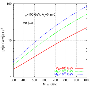
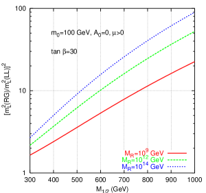
(a)	(b)

Figure 1: The ratio of the (2,1) element of $\left[m^{2}_{\widetilde{L}}(RG)/m^{2}_{\widetilde{L}}(LL)\right]^{2}$ as a function of $M_{1/2}$ at $\tan\beta=3.0$ (a) and $\tan\beta=30.0$ (b). In the two panels we fixed $m_{0}=100~{}\mbox{\rm GeV}$, $A_{0}=0$ and $\mu>0$.

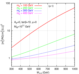
(a)	(b)

Figure 2: The ratio of the (3,2) (a) element and of the of (2,1) (b) element of $\left[m^{2}_{\widetilde{L}}(RG)/m^{2}_{\widetilde{L}}(LL)\right]^{2}$ as a function of $M_{1/2}$ at $\tan\beta=10.0$. In the two panels we fixed $M_{R}=10^{11}~{}\mbox{\rm GeV}$, $A_{0}=0$ and $\mu>0$.

5.2 Lepton Flavor Violating Processes

In this section we turn to the main topic of interest in the present work: the size of the corrections induced by the full RG running in the rates of LFV processes. We compare here the results obtained inserting the leading log approximation for $\left(m^{2}_{\widetilde{\scriptscriptstyle L}}(LL)\right)_{ji}$, Eq. (27), in the full mass matrix formulae [23] given in Appendix B, see Eqs. (73)-(82), with the exact RG running result for the LFV decay branching ratios. We would like to emphasize that the results for the off-diagonal slepton mass terms derived in leading log approximation and by exact RG running are included in the slepton mass matrix which after that is diagonalized and the mass eigenstate scalar leptons and the corresponding mixing matrix determined. The letter are used in the calculations of ${\rm BR}(\l_{j}\to l_{i}\gamma)$. Note that the branching ratios of the LFV processes depend on the eigenvalues of the the slepton mass matrix and on the elements of the matrix which diagonalize it (see Appendix B); they do not depend directly on the off-diagonal entries of the slepton mass matrix. Therefore we will in general get results which differ from the ones expected on the basis of the results reported in the preceding section.

In Fig. 3 we plot as functions of $M_{1/2}$ the full RG results (solid red lines) and the results obtained within the leading log approximation (dashed green lines) for two values of $m_{0}$, $m_{0}=100;~{}300~{}\mbox{\rm GeV}$, at $\tan\beta=30.0$ and $M_{R}=10^{11}~{}\mbox{\rm GeV}$. We see that, in agreement with was obtained in the preceding section, the increasing of $m_{0}$ reduces the RG corrections: the RG flow is mainly driven by $m_{0}$ and the corrections due to $M_{1/2}$ become less important. We get, for $m_{0}=100~{}\mbox{\rm GeV}$, a correction of roughly one order of magnitude at large $M_{1/2}\approx 1~{}\mbox{\rm TeV}$, while for the $m_{0}=300~{}\mbox{\rm GeV}$ case the effect reduces to a factor of two. We notice, comparing panels (a) and (b), that the difference between the exact RG results and those obtained in the leading log approximation is larger at lower values of $\tan\beta$.

Fig. 4 shows the effect on ${\rm BR}(\mu\to e\gamma)$ of changing the right-handed heavy neutrino mass $M_{R}$ as a function of $M_{1/2}$. We used $m_{0}=100~{}\mbox{\rm GeV}$, $A_{0}=0$, $\mu>0$ and $\tan\beta=30.0$, taking $M_{R}=10^{9}~{}\mbox{\rm GeV},\ 10^{12}~{}\mbox{\rm GeV}$ and $10^{14}~{}\mbox{\rm GeV}$. We find that the size of the difference between the exact RG result and the leading log approximation one depends weakly on $M_{R}$. At large $M_{1/2}$ we always get a discrepancy between leading log and full RG results of about one order of magnitude (notice the different scale with respect to the preceding figure). Here, again, the effect is enhanced at lower $\tan\beta$ (see panel (b)).

Finally, we would like to emphasize that although the change in the LFV decay rates we find using the exact RG results in comparison with those obtained in the leading log approximation are within one order of magnitude, it would be mandatory to use the former in order to draw conclusions concerning the SUSY sector if any LF violating decay will be observed and its branching ratio measured. As it follows from Figs. 4, if we fix ${\rm BR}(\mu\rightarrow e\gamma)$, for instance, we could make an error of up to $\approx 50\%$ using the leading log approximation in deriving a lower bound on $M_{1/2}$.

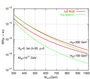
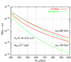
(a)	(b)

Figure 3: The branching ratio for the LFV process ${\rm BR}(\mu\rightarrow e\gamma)$ as a function of $M_{1/2}$ at $m_{0}=100~{}\mbox{\rm GeV}$ and $m_{0}=100~{}\mbox{\rm GeV}$ in the full RG (solid red lines) and leading logarithmic approximation (dashed green lines). We set in the figures $M_{R}=10^{11}~{}\mbox{\rm GeV}$, $A_{0}=0$, $\mu>0$ and $\tan\beta=30.0$ (a) and $\tan\beta=3.0$ (b).

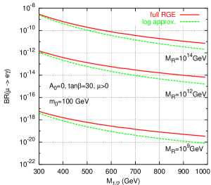
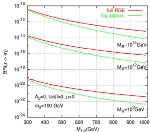
(a)	(b)

Figure 4: The branching ratio for the LFV process ${\rm BR}(\mu\rightarrow e\gamma)$ as a function of $M_{1/2}$ at $M_{R}=10^{9}~{}\mbox{\rm GeV},\ 10^{12}~{}\mbox{\rm GeV}$ and $10^{14}~{}\mbox{\rm GeV}$ in the full RG (solid red lines) and leading logarithmic approximation (dashed green lines). We set in the figures $m_{0}=100~{}\mbox{\rm GeV}$, $A_{0}=0$, $\mu>0$ and $\tan\beta=30.0$ (a) and $\tan\beta=3.0$ (b).

5.3 Exact RG Evolution Effects from $\mu$ and $A_{0}$

In this section we deal with two other high energy input “parameters” which are neglected in the leading log approximation, namely the sign of the scalar trilinear coupling $A_{0}$ and of $\mu$. We depict in the left panel of Fig. 5 the results we get, in the full RG running computation, for $A_{0}=0$ (solid red line), $A_{0}=\pm 1~{}\mbox{\rm TeV}$ (resp. lower and upper dashed green lines) and $A_{0}=\pm 2~{}\mbox{\rm TeV}$ (resp. lower and upper dotted blue lines). In the figure we fixed for definiteness $\tan\beta=10.0$, $M_{R}=10^{11}~{}\mbox{\rm GeV}$ and $m_{0}=200~{}\mbox{\rm GeV}$. We see that instead negative values of the trilinear coupling generically enhance, by up to roughly a factor of $5$, the LFV branching ratios. Flipping the sign of $\mu$ gives rise to smaller corrections (panel (b)). In particular, we find that at low $m_{0}$, values of $\mu>0$ slightly suppress the LFV branching ratios, while at larger $m_{0}$ a mild enhancement takes place.

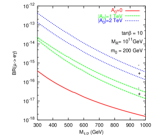
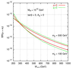
(a)	(b)

Figure 5: (a): ${\rm BR}(\mu\rightarrow e\gamma)$ as a function of $M_{1/2}$ at $A_{0}=0,\ \pm 1~{}\mbox{\rm TeV},\ \pm 2~{}\mbox{\rm TeV}$ for $\tan\beta=10.0$, $M_{R}=10^{11}~{}\mbox{\rm GeV}$ and $m_{0}=200~{}\mbox{\rm GeV}$. (b): The same at $m_{0}=100~{}\mbox{\rm GeV}$ (lower lines) and $m_{0}=500~{}\mbox{\rm GeV}$ (upper lines) at $\mu>0$ (dashed green lines) and $\mu<0$ (solid red lines), for $\tan\beta=3.0$, $M_{R}=10^{12}~{}\mbox{\rm GeV}$.

5.4 The Coannihilation region

We provide in this section some results concerning the branching ratios of LFV in a particular region of the mSUGRA parameter space, namely the one where coannihilations between the lightest neutralino and the lightest stau (the next-to-lightest SUSY particle) concur in reducing the neutralino relic density within the current observational cold dark matter content of the universe. In Fig. 6 we study the ${\rm BR}(\mu\rightarrow e\gamma)$ (a) and ${\rm BR}(\tau\rightarrow\mu\gamma)$ (b) as a function of the neutralino mass $m_{\chi}$ along the “coannihilation corridor” at fixed $\tan\beta=30.0$ for three different values of $M_{R}=10^{9}~{}\mbox{\rm GeV},\ 10^{11}~{}\mbox{\rm GeV}$ and $10^{13}~{}\mbox{\rm GeV}$. We recall that in mSUGRA $m_{\chi}\approx 0.4M_{1/2}$. Notice that for sufficiently low values of $M_{R}$ the computed ${\rm BR}(\mu\rightarrow e\gamma)$ is always below the current experimental bounds, while putative lower bounds on $m_{\chi}$ can be drawn for larger $M_{R}$. In the case of ${\rm BR}(\tau\rightarrow\mu\gamma)$ we always get results far below (at least two orders of magnitude) the current experimental bound. As was natural to expect, and as is shown in Fig. 7 (a), lowering $\tan\beta$ yields a quadratic suppression in the LFV Branching ratios, which appear to be in all cases well below the current experimental sensitivity. Finally, in Fig. 7 (b) we summarize our results showing the $M_{1/2}$ ranges dictated by cosmological and phenomenological requirements. These constraints, leading to smaller allowed $M_{1/2}$ for $\mu>0$ indicate that this last case is favored to produce larger LFV decay rates, which may be in the range of sensitivity of the next generation experiments.

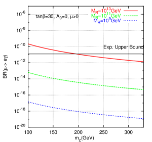
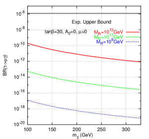
(a)	(b)

Figure 6: (a): ${\rm BR}(\mu\rightarrow e\gamma)$ as a function of $m_{\chi}$ in the stau coannihilation strip at $\tan\beta=30.0$, $\mu>0$ and $A_{0}=0$, for $M_{R}=10^{9}~{}\mbox{\rm GeV}$, $10^{11}~{}\mbox{\rm GeV}$ and $10^{13}~{}\mbox{\rm GeV}$. (b): the same for ${\rm BR}(\tau\rightarrow\mu\gamma)$.

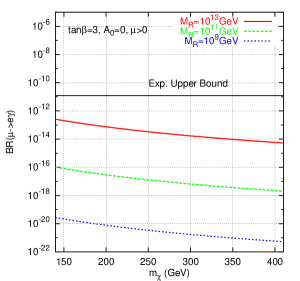
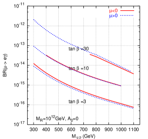
(a)	(b)

Figure 7: (a): Same as in Fig.6 (a) but at $\tan\beta=3.0$. (b) ${\rm BR}(\mu\rightarrow e\gamma)$ along the cosmologically and phenomenologically viable coannihilation strips for both signs of $\mu$ and various $\tan\beta$. Results at $\tan\beta=3.0$ are ruled out by the bound on $m_{h}$ set by LEP2, but we nonetheless report them for completeness.

5.5 A Candidate for the Effective SUSY Mass $m_{\scriptscriptstyle S}$

The branching ratio for the processes $l_{j}\rightarrow l_{i}\gamma$ is often quoted in the literature in the mass insertion and leading log approximations as

$${\rm BR}(l_{j}\rightarrow l_{i}\gamma)\simeq\frac{\alpha^{3}}{G_{\scriptscriptstyle F}^{2}}\frac{\left|\left(m_{\widetilde{\scriptscriptstyle L}}^{2}(LL)\right)_{ji}\right|^{2}}{m_{\scriptscriptstyle S}^{8}}\tan^{2}\beta\hskip 5.69054pt,$$ (28)

where $m_{\scriptscriptstyle S}$ is a typical mass of superparticles, $\alpha\simeq 1/128$ and $\left(m_{\widetilde{\scriptscriptstyle L}}^{2}(LL)\right)_{ji}$ is given by Eq. (27). The problem with this formula is that there is no prescription for $m_{\scriptscriptstyle S}$ in terms of the fundamental SUSY and soft breaking parameters of the theory, and the dependence on $m_{\scriptscriptstyle S}$ is so strong that the predictions for ${\rm BR}(l_{j}\rightarrow l_{i}\gamma)$ depend drastically on what one uses for $m_{\scriptscriptstyle S}$: $m_{\scriptscriptstyle S}=m_{0}$, or $m_{\scriptscriptstyle S}=m_{\widetilde{\nu}}$, or $m_{\scriptscriptstyle S}=\sqrt{\mu M_{1/2}}$. The three indicated choices will give completely different predictions for the branching ratios of interest. Notice that if we underestimate $m_{\scriptscriptstyle S}$ by just a factor of two we are overestimating the branching ratios by more than two orders of magnitude.

We have found that the expression (28) with $\left(m_{\widetilde{\scriptscriptstyle L}}^{2}(LL)\right)_{ji}$ given by Eq. (27) represents an excellent approximation to the exact RG result if for $m_{\scriptscriptstyle S}$ one uses

$$m_{\scriptscriptstyle S}^{8}\simeq 0.5\ m_{0}^{2}\ M_{1/2}^{2}\ \left(m_{0}^{2}\ +\ 0.6\ M_{1/2}^{2}\right)^{2}\hskip 5.69054pt.$$ (29)

In Fig. 8 we compare the predictions for $m_{\scriptscriptstyle S}^{8}$ obtained from (28) and the exact RG result for ${\rm BR}(l_{j}\rightarrow l_{i}\gamma)$ with that given by Eq. (29). In general, we find that our fit formula (29) slightly underestimates $m_{\scriptscriptstyle S}$ at low $M_{1/2}$ and large $m_{0}$, and somewhat overestimates it at large $M_{1/2}$ and small $m_{0}$. The deviations are, however, always relatively small, and the overall dependence of $m_{\scriptscriptstyle S}^{8}$ on $m_{0}$ and $M_{1/2}$ is everywhere reproduced rather accurately.

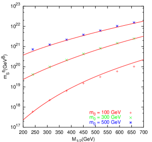
Figure 8: A fit to $m_{\scriptscriptstyle S}^{8}$. The lines correspond to Eq. (29), while the points to the value extracted from the full RGE numerical results and Eq. (28). In this plot we use $M_{R}=10^{14}~{}\mbox{\rm GeV}$, $\tan\beta=3$ and $A_{0}=0$.

6 Conclusions

We have shown that the off-diagonal elements of the slepton mass matrix obtained by RG running deviate significantly – at low $m_{0}$ and large $M_{1/2}$ – from the values given by the leading logarithmic approximation. The exact result is always larger than the approximated one and this difference increases for larger $M_{R}$. As a consequence, in the leading log approximation the predictions for $\mu\rightarrow e\gamma$ and $\tau\rightarrow\mu\gamma$ can be underestimated by a factor $\sim 10$. We pointed out that, even when this factor is smaller, it is relevant if one wants to use ${\rm BR}(\mu\rightarrow e\gamma)$ and ${\rm BR}(\tau\rightarrow\mu\gamma)$ to constrain the SUSY parameter space. These branching ratios were found to depend on the sign of $A_{0}$ and of $\mu$ as well.

We also studied the behavior of ${\rm BR}(\mu\rightarrow e\gamma)$ and ${\rm BR}(\tau\rightarrow\mu\gamma)$ along the cosmologically determined “coannihilation strips”. Our results show that the present experimental bound on $\mu\rightarrow e\gamma$ can exclude only regions with large $M_{R}$ ($M_{R}\geq 10^{13}~{}\mbox{\rm GeV}$), while $\tau\rightarrow\mu\gamma$ is always allowed. Finally, we proposed a simple parametrization in terms of $m_{0}$ and $M_{1/2}$ for the effective SUSY mass parameter $m_{\scriptscriptstyle S}$ which enters into the simple expression for ${\rm BR}(l_{j}\rightarrow l_{i}\gamma)$ derived in the leading log and mass insertion approximations (see Eqs. (27)-(29)). This allows to reproduce the exact RG results for ${\rm BR}(l_{j}\rightarrow l_{i}\gamma)$ with high precision.

Appendix A Renormalization Group Equations

From the GUT scale $M_{\rm\scriptscriptstyle GUT}$ down to the universal $M_{\rm\scriptscriptstyle R}$ scale we use the one-loop MSSM renormalization group equation [24] of the gauge coupling constants, the three gaugino mass parameters, the Yukawa coupling constant matrices, $Y_{u}$, $Y_{d}$, $Y_{e}$, $Y_{\nu}$, and the right-handed neutrino mass matrix, $M_{\scriptscriptstyle R}$, and the soft supersymmetry breaking mass terms and trilinear parameters, $A$.

The gauge coupling constants (especially $g_{2}$ running effect) and the gaugino mass terms (as well $M_{2}$ running effect), play important rôle in the calculation of the lepton flavor violation processes, therefore a part of the two-loop $\beta$ functions are adopted in our computations. We present at first the non-supersymetric part of the renormalization from the GUT scale $M_{\rm\scriptscriptstyle GUT}$ to the universal $M_{\scriptscriptstyle R}$ scale:

$$16\pi^{2}\frac{d}{dt}~{}g_{1} \!=\! \frac{33}{5}\,g_{1}^{3}+\frac{g_{1}^{3}}{16\pi^{2}}\left(\frac{199}{25}g_{1}^{2}+\frac{27}{5}g^{2}_{2}+\frac{88}{5}g_{3}^{2}\right)\hskip 5.69054pt,$$ (30)

$$16\pi^{2}\frac{d}{dt}~{}g_{2} \!=\! \,g_{2}^{3}+\frac{g_{2}^{3}}{16\pi^{2}}\left(\frac{9}{5}g_{1}^{2}+25g^{2}_{2}+24g_{3}^{2}\right)\hskip 5.69054pt,$$ (31)

$$16\pi^{2}\frac{d}{dt}~{}g_{3} \!=\! -3\,g_{3}^{3}+\frac{g_{3}^{3}}{16\pi^{2}}\left(\frac{1}{5}g_{1}^{2}+9g^{2}_{2}+14g_{3}^{2}\right)\hskip 5.69054pt,$$ (32)

$$16\pi^{2}\frac{d}{dt}Y_{u_{ij}} \!=\! \left\{-\frac{13}{15}g_{1}^{2}-3g_{2}^{2}-\frac{16}{3}g_{3}^{2}+3\,{\rm Tr}(Y_{u}Y_{u}^{\dagger})+{\rm Tr}(Y_{\nu}Y_{\nu}^{\dagger})\right\}Y_{u_{ij}}$$ (33)

$$\;+3\,(Y_{u}Y_{u}^{\dagger}Y_{u})_{ij}+(Y_{u}Y_{d}^{\dagger}Y_{d})_{ij}\hskip 5.69054pt,$$

$$16\pi^{2}\frac{d}{dt}Y_{d_{ij}} \!=\! \left\{-\frac{7}{15}g_{1}^{2}-3g_{2}^{2}-\frac{16}{3}g_{3}^{2}+3\,{\rm Tr}(Y_{d}Y_{d}^{\dagger})+{\rm Tr}(Y_{e}Y_{e}^{\dagger})\right\}Y_{d_{ij}}$$ (34)

$$+\;3\,(Y_{d}Y_{d}^{\dagger}Y_{d})_{ij}+(Y_{d}Y_{u}^{\dagger}Y_{u})_{ij}\hskip 5.69054pt,$$

$$16\pi^{2}\frac{d}{dt}Y_{e_{ij}} \!=\! \left\{-\frac{9}{5}g_{1}^{2}-3g_{2}^{2}+3\,{\rm Tr}(Y_{d}Y_{d}^{\dagger})+{\rm Tr}(Y_{e}Y_{e}^{\dagger})\right\}Y_{e_{ij}}$$ (35)

$$+3\,\left(Y_{e}Y_{e}^{\dagger}Y_{e}\right)_{ij}+\left(Y_{e}Y_{\nu}^{\dagger}Y_{\nu}\right)_{ij}\hskip 5.69054pt,$$

$$16\pi^{2}\frac{d}{dt}Y_{\nu_{ij}} \!=\! \left\{-\frac{3}{5}g_{1}^{2}-3g_{2}^{2}+3\,{\rm Tr}\left(Y_{u}Y_{u}^{\dagger}\right)+{\rm Tr}\left(Y_{\nu}Y_{\nu}^{\dagger}\right)\right\}Y_{\nu_{ij}}$$ (36)

$$+3\,\left(Y_{\nu}Y_{\nu}^{\dagger}Y_{\nu}\right)_{ij}+\left(Y_{\nu}Y_{e}^{\dagger}Y_{e}\right)_{ij}\hskip 5.69054pt,$$

$$16\pi^{2}\frac{d}{dt}M_{R_{ij}} \!=\! 2\left(M_{R}Y^{\dagger}_{\nu}Y_{\nu}\right)_{ij}+2\left(Y_{\nu}Y^{\dagger}_{\nu}M_{R}\right)_{ij}\hskip 5.69054pt.$$ (37)

Here are the renormalization group equations of the gaugino mass terms, the soft mass terms and the trilinear parameters as well the up-type and down-type Higgs mass terms, respectively. Note that we take into account the two-loop $\beta$ function accuracy only for the gaugino mass terms:

$$16\pi^{2}\frac{d}{dt}M_{1} \!=\! \frac{66}{5}\,g_{1}^{2}M_{1}+\frac{2g_{1}^{2}}{16\pi^{2}}\left\{\frac{199}{5}g^{2}_{1}\left(2M_{1}\right)\right.$$ (38)

$$\left.+\frac{27}{5}g_{2}^{2}\left(M_{1}+M_{2}\right)+\frac{88}{5}g_{3}^{2}\left(M_{1}+M_{3}\right)\right\}\hskip 5.69054pt,$$

$$16\pi^{2}\frac{d}{dt}M_{2} \!=\! 2\,g_{2}^{2}M_{2}+\frac{2g_{2}^{2}}{16\pi^{2}}\left\{\frac{9}{5}g^{2}_{1}\left(M_{1}+M_{2}\right)\right.$$ (39)

$$\left.+25g_{2}^{2}\left(2M_{2}\right)+24g_{3}^{2}\left(M_{2}+M_{3}\right)\right\}\hskip 5.69054pt,$$

$$16\pi^{2}\frac{d}{dt}M_{3} \!=\! -6\,g_{3}^{2}M_{3}+\frac{2g_{3}^{2}}{16\pi^{2}}\left\{\frac{11}{5}g^{2}_{1}\left(M_{1}+M_{3}\right)\right.$$ (40)

$$\left.+9g_{2}^{2}\left(M_{2}+M_{3}\right)+14g_{3}^{2}\left(2M_{3}\right)\right\}\hskip 5.69054pt,$$

$$16\pi^{2}\frac{d}{dt}\left(m^{2}_{\widetilde{\scriptscriptstyle Q}}\right)_{ij} \!=\! -\left(\frac{2}{15}g_{1}^{2}\left|M_{1}\right|^{2}+6g_{2}^{2}\left|M_{2}\right|^{2}+\frac{32}{3}g_{3}^{2}\left|M_{3}\right|^{2}\right)\delta_{ij}+\frac{1}{5}g_{1}^{2}~{}S~{}\delta_{ij}$$ (41)

$$+\left(m^{2}_{\widetilde{\scriptscriptstyle Q}}Y_{u}^{\dagger}Y_{u}+m^{2}_{\widetilde{\scriptscriptstyle Q}}Y_{d}^{\dagger}Y_{d}+Y_{u}^{\dagger}Y_{u}m^{2}_{\widetilde{\scriptscriptstyle Q}}+Y_{d}^{\dagger}Y_{d}m^{2}_{\widetilde{\scriptscriptstyle Q}}\right)_{ij}$$

$$+2\left(Y_{u}^{\dagger}m^{2}_{\widetilde{u}}Y_{u}+{m}^{2}_{H_{u}}Y_{u}^{\dagger}Y_{u}+A_{u}^{\dagger}A_{u}\right)_{ij}$$

$$+2\left(Y_{d}^{\dagger}m^{2}_{\widetilde{d}}Y_{d}+{m}^{2}_{H_{d}}Y_{d}^{\dagger}Y_{d}+A_{d}^{\dagger}A_{d}\right)_{ij}\hskip 5.69054pt,$$

$$16\pi^{2}\frac{d}{dt}\left(m^{2}_{\widetilde{u}}\right)_{ij} \!=\! -\left(\frac{32}{15}g_{1}^{2}\left|M_{1}\right|^{2}+\frac{32}{3}g_{3}^{2}\left|M_{3}\right|^{2}\right)\delta_{ij}-\frac{4}{5}g_{1}^{2}~{}S~{}\delta_{ij}$$ (42)

$$+2\left(m^{2}_{\widetilde{u}}Y_{u}Y_{u}^{\dagger}+Y_{u}Y_{u}^{\dagger}m^{2}_{\widetilde{u}}\right)_{ij}$$

$$+4\left(Y_{u}m^{2}_{\widetilde{\scriptscriptstyle Q}}Y_{u}^{\dagger}+{m}^{2}_{H_{u}}Y_{u}Y_{u}^{\dagger}+A_{u}A_{u}^{\dagger}\right)_{ij}\hskip 5.69054pt,$$

$$16\pi^{2}\frac{d}{dt}\left(m^{2}_{\widetilde{d}}\right)_{ij} \!=\! -\left(\frac{8}{15}g_{1}^{2}\left|M_{1}\right|^{2}+\frac{32}{3}g_{3}^{2}\left|M_{3}\right|^{2}\right)\delta_{ij}+\frac{2}{5}g_{1}^{2}~{}S~{}\delta_{ij}$$ (43)

$$+2\left(m^{2}_{\widetilde{d}}Y_{d}Y_{d}^{\dagger}+Y_{d}Y_{d}^{\dagger}m^{2}_{\widetilde{d}}\right)_{ij}$$

$$+4\left(Y_{d}m^{2}_{\widetilde{\scriptscriptstyle Q}}Y_{d}^{\dagger}+{m}^{2}_{H_{d}}Y_{d}Y_{d}^{\dagger}+A_{d}A_{d}^{\dagger}\right)_{ij}\hskip 5.69054pt,$$

$$16\pi^{2}\frac{d}{dt}\left(m^{2}_{\widetilde{\scriptscriptstyle L}}\right)_{ij} \!=\! -\left(\frac{6}{5}g_{1}^{2}\left|M_{1}\right|^{2}+6g_{2}^{2}\left|M_{2}\right|^{2}\right)\delta_{ij}-\frac{3}{5}g_{1}^{2}~{}S~{}\delta_{ij}$$ (44)

$$+\left(m^{2}_{\widetilde{\scriptscriptstyle L}}Y_{e}^{\dagger}Y_{e}+m^{2}_{\widetilde{\scriptscriptstyle L}}Y_{\nu}^{\dagger}Y_{\nu}+Y_{e}^{\dagger}Y_{e}m^{2}_{\widetilde{\scriptscriptstyle L}}+Y_{\nu}^{\dagger}Y_{\nu}m^{2}_{\widetilde{\scriptscriptstyle L}}\right)_{ij}$$

$$+2\left(Y_{e}^{\dagger}m^{2}_{\widetilde{e}}Y_{e}+{m}^{2}_{H_{d}}Y_{e}^{\dagger}Y_{e}+A_{e}^{\dagger}A_{e}\right)_{ij}$$

$$+2\left(Y_{\nu}^{\dagger}m^{2}_{\widetilde{\scriptscriptstyle\nu}}Y_{\nu}+{m}^{2}_{H_{u}}Y_{\nu}^{\dagger}Y_{\nu}+A_{\nu}^{\dagger}A_{\nu}\right)_{ij}\hskip 5.69054pt,$$

$$16\pi^{2}\frac{d}{dt}\left(m^{2}_{\widetilde{e}}\right)_{ij} \!=\! -\frac{24}{5}g_{1}^{2}\left|M_{1}\right|^{2}\delta_{ij}+\frac{6}{5}g_{1}^{2}~{}S~{}\delta_{ij}+2\left(m^{2}_{\widetilde{e}}Y_{e}Y_{e}^{\dagger}+Y_{e}Y_{e}^{\dagger}m^{2}_{\widetilde{e}}\right)_{ij}$$ (45)

$$+4\left(Y_{e}m^{2}_{\scriptscriptstyle\widetilde{L}}Y_{e}^{\dagger}+{m}^{2}_{H_{d}}Y_{e}Y_{e}^{\dagger}+A_{e}A_{e}^{\dagger}\right)_{ij}\hskip 5.69054pt,$$

$$16\pi^{2}\frac{d}{dt}\left(m^{2}_{\widetilde{\nu}}\right)_{ij} \!=\! 2\left(m^{2}_{\widetilde{\nu}}Y_{\nu}Y_{\nu}^{\dagger}+Y_{\nu}Y_{\nu}^{\dagger}m^{2}_{\widetilde{\nu}}\right)_{ij}+4\left(Y_{\nu}m^{2}_{\widetilde{L}}Y_{\nu}^{\dagger}+{m}^{2}_{H_{u}}Y_{\nu}Y_{\nu}^{\dagger}+A_{\nu}A_{\nu}^{\dagger}\right)_{ij}\hskip 5.69054pt,$$ (46)

$$16\pi^{2}\frac{d}{dt}A_{e_{ij}} \!=\! \left\{-\frac{9}{5}g_{1}^{2}-3g_{2}^{2}+3{\rm Tr}(Y_{d}^{\dagger}Y_{d})+{\rm Tr}(Y_{e}^{\dagger}Y_{e})\right\}A_{e_{ij}}$$ (47)

$$+2\left\{\frac{9}{5}g_{1}^{2}M_{1}+3g_{2}^{2}M_{2}+3{\rm Tr}(Y_{d}^{\dagger}A_{d})+{\rm Tr}(Y_{e}^{\dagger}A_{e})\right\}Y_{e_{ij}}$$

$$+4\left(Y_{e}Y_{e}^{\dagger}A_{e}\right)_{ij}+5\left(A_{e}Y_{e}^{\dagger}Y_{e}\right)_{ij}+2\left(Y_{e}Y_{\nu}^{\dagger}A_{\nu}\right)_{ij}+\left(A_{e}Y_{\nu}^{\dagger}Y_{\nu}\right)_{ij}\hskip 5.69054pt,$$

$$16\pi^{2}\frac{d}{dt}A_{\nu_{ij}} \!=\! \left\{-\frac{3}{5}g_{1}^{2}-3g_{2}^{2}+3{\rm Tr}(Y_{u}^{\dagger}Y_{u})+{\rm Tr}(Y_{\nu}^{\dagger}Y_{\nu})\right\}A_{\nu_{ij}}$$ (48)

$$+2\left\{\frac{3}{5}g_{1}^{2}M_{1}+3g_{2}^{2}M_{2}+3{\rm Tr}(Y_{u}^{\dagger}A_{u})+{\rm Tr}(Y_{\nu}^{\dagger}A_{\nu})\right\}Y_{\nu_{ij}}$$

$$+4(Y_{\nu}Y_{\nu}^{\dagger}A_{\nu})_{ij}+5(A_{\nu}Y_{\nu}^{\dagger}Y_{\nu})_{ij}+2(Y_{\nu}Y_{e}^{\dagger}A_{e})_{ij}+(A_{\nu}Y_{e}^{\dagger}Y_{e})_{ij}\hskip 5.69054pt,$$

$$16\pi^{2}\frac{d}{dt}A_{u_{ij}} = \left\{-\frac{13}{15}g_{1}^{2}-3g_{2}^{2}-\frac{16}{3}g_{3}^{2}+3{\rm Tr}(Y_{u}^{\dagger}Y_{u})+{\rm Tr}(Y_{\nu}^{\dagger}Y_{\nu})\right\}A_{u_{ij}}$$ (49)

$$+2\left\{\frac{13}{15}g_{1}^{2}M_{1}+3g_{2}^{2}M_{2}+\frac{16}{3}g_{3}^{2}M_{3}+3{\rm Tr}(Y_{u}^{\dagger}A_{u})+{\rm Tr}(Y_{\nu}^{\dagger}A_{\nu})\right\}Y_{u_{ij}}$$

$$+4(Y_{u}Y_{u}^{\dagger}A_{u})_{ij}+5(A_{u}Y_{u}^{\dagger}Y_{u})_{ij}+2(Y_{u}Y_{d}^{\dagger}A_{d})_{ij}+(A_{u}Y_{d}^{\dagger}Y_{d})_{ij}\hskip 5.69054pt,$$

$$16\pi^{2}\frac{d}{dt}A_{d_{ij}} = \left\{-\frac{7}{15}g_{1}^{2}-3g_{2}^{2}-\frac{16}{3}g_{3}^{2}+3{\rm Tr}(Y_{d}^{\dagger}Y_{d})+{\rm Tr}(Y_{e}^{\dagger}Y_{e})\right\}A_{d_{ij}}$$ (50)

$$+2\left\{\frac{7}{15}g_{1}^{2}M_{1}+3g_{2}^{2}M_{2}+\frac{16}{3}g_{3}^{2}M_{3}+3{\rm Tr}(Y_{d}^{\dagger}A_{d})+{\rm Tr}(Y_{e}^{\dagger}A_{e})\right\}Y_{d_{ij}}$$

$$+4(Y_{d}Y_{d}^{\dagger}A_{d})_{ij}+5(A_{d}Y_{d}^{\dagger}Y_{d})_{ij}+2(Y_{d}Y_{u}^{\dagger}A_{u})_{ij}+(A_{d}Y_{u}^{\dagger}Y_{u})_{ij}\hskip 5.69054pt,$$

$${16\pi^{2}}\frac{d}{dt}(m^{2}_{H_{u}}) = -\left(\frac{6}{5}g^{2}_{1}\left|M_{1}\right|^{2}+6g^{2}_{2}\left|M_{2}\right|^{2}\right)+\frac{3}{5}g_{1}^{2}S$$ (51)

$$+6\,{\rm{\rm Tr}}\left(m^{2}_{\widetilde{Q}}Y^{\dagger}_{u}Y_{u}+Y^{\dagger}_{u}(m^{2}_{\widetilde{u}}+m^{2}_{H_{u}})Y_{u}+A^{\dagger}_{u}A_{u}\right)$$

$$+2\,{\rm Tr}\left(m^{2}_{\widetilde{\scriptscriptstyle L}}Y^{\dagger}_{\nu}Y_{\nu}+Y^{\dagger}_{\nu}(m^{2}_{\widetilde{\nu}}+m^{2}_{H_{u}})Y_{\nu}+A^{\dagger}_{\nu}A_{\nu}\right)\hskip 5.69054pt,$$

$${16\pi^{2}}\frac{d}{dt}(m^{2}_{H_{d}}) = -\left(\frac{6}{5}g^{2}_{1}\left|M_{1}\right|^{2}+6g^{2}_{2}\left|M_{2}\right|^{2}\right)-\frac{3}{5}g_{1}^{2}S$$ (52)

$$+6\,{\rm Tr}\left(m^{2}_{\widetilde{Q}}Y^{\dagger}_{d}Y_{d}+Y^{\dagger}_{d}(m^{2}_{\widetilde{d}}+m^{2}_{H_{d}})Y_{d}+A^{\dagger}_{d}A_{d}\right)$$

$$+2\,{\rm Tr}\left(m^{2}_{\widetilde{\scriptscriptstyle L}}Y^{\dagger}_{e}Y_{e}+Y^{\dagger}_{e}(m^{2}_{\widetilde{e}}+m^{2}_{H_{d}})Y_{e}+A_{e}^{\dagger}A_{e}\right)\hskip 5.69054pt,$$

where

$$S={\rm Tr}(m_{\widetilde{Q}}^{2}+m_{\widetilde{d}}^{2}-2m_{\widetilde{u}}^{2}-m_{\widetilde{L}}^{2}+m_{\widetilde{e}}^{2})-{m}^{2}_{H_{d}}+{m}^{2}_{H_{u}}\hskip 5.69054pt,$$ (53)

and we have used the GUT convention for the $U(1)$ gauge coupling constant, $g_{1}$, and $t=\ln\mu$ where $\mu$ is denoted as the renormalization point.

Appendix B Notations in the MSSM

In this appendix we set the notations and conventions for the computation of LFV processes. Note that we follow the Appendix B of ref. [23].

The chargino mass matrix has the following form:

$$-\mathscr{L}_{m}=\left(\overline{\widetilde{W}^{-}_{\scriptscriptstyle R}}~{}\overline{\widetilde{H}^{-}_{2{\scriptscriptstyle R}}}\right)M_{\scriptscriptstyle C}\left(\begin{array}[]{c}\widetilde{W}^{-}_{\scriptscriptstyle L}\\ \widetilde{H}_{1{\scriptscriptstyle L}}^{-}\end{array}\right)+h.c.\hskip 5.69054pt,$$ (54)

where

$$M_{\scriptscriptstyle C}=\left(\begin{array}[]{cc}M_{2}&\sqrt{2}m_{W}\cos\beta\\ \sqrt{2}m_{W}\sin\beta&\mu\end{array}\right)\hskip 5.69054pt.$$ (55)

This matrix can be diagonalized by two $2\times 2$ real orthogonal matrices $O_{\scriptscriptstyle L}$ and $O_{\scriptscriptstyle R}$ according to:

$$O_{\scriptscriptstyle R}M_{\scriptscriptstyle C}O_{\scriptscriptstyle L}^{\sf T}={\rm diagonal}\hskip 5.69054pt.$$ (56)

If we define

$$\left(\begin{array}[]{c}\widetilde{\chi}^{-}_{1{\scriptscriptstyle L}}\\ \widetilde{\chi}^{-}_{2{\scriptscriptstyle L}}\end{array}\right)=O_{\scriptscriptstyle L}\left(\begin{array}[]{c}\widetilde{W}^{-}_{\scriptscriptstyle L}\\ \widetilde{H}^{-}_{1{\scriptscriptstyle L}}\end{array}\right)\hskip 5.69054pt,\hskip 28.45274pt\left(\begin{array}[]{c}\widetilde{\chi}^{-}_{1{\scriptscriptstyle R}}\\ \widetilde{\chi}^{-}_{2{\scriptscriptstyle R}}\end{array}\right)=O_{\scriptscriptstyle R}\left(\begin{array}[]{c}\widetilde{W}^{-}_{\scriptscriptstyle R}\\ \widetilde{H}^{-}_{2{\scriptscriptstyle R}}\end{array}\right)\hskip 5.69054pt,$$ (57)

then

$${\widetilde{\chi}}^{-}_{\scriptscriptstyle A}={\widetilde{\chi}}^{-}_{{\scriptscriptstyle AL}}+{\widetilde{\chi}}^{-}_{{\scriptscriptstyle AR}}$$ (58)

forms a Dirac fermion with mass $M_{{\widetilde{\chi}}^{-}_{\scriptscriptstyle A}}$.

The mass matrix of the neutralino sector is given by

$$-\mathscr{L}_{m}=\frac{1}{2}\left({\widetilde{B}}_{L}{\widetilde{W}}^{0}_{L}{\widetilde{H}}^{0}_{1L}{\widetilde{H}}^{0}_{2L}\right)M_{N}\left(\begin{array}[]{c}{\widetilde{B}}_{L}\\ {\widetilde{W}}^{0}_{L}\\ {\widetilde{H}}^{0}_{1L}\\ {\widetilde{H}}^{0}_{2L}\end{array}\right)+h.c.\hskip 5.69054pt,$$ (59)

where

$$M_{\scriptscriptstyle N}=\left(\begin{array}[]{cccc}M_{1}&0&-m_{Z}\sin\theta_{W}\cos\beta&m_{Z}\sin\theta_{W}\sin\beta\\ 0&M_{2}&m_{Z}\cos\theta_{W}\cos\beta&-m_{Z}\cos\theta_{W}\sin\beta\\ -m_{Z}\sin\theta_{W}\cos\beta&m_{Z}\cos\theta_{W}\cos\beta&0&-\mu\\ m_{Z}\sin\theta_{W}\sin\beta&-m_{Z}\cos\theta_{W}\sin\beta&-\mu&0\end{array}\right)\hskip 5.69054pt.$$ (60)

We can diagonalize $M_{\scriptscriptstyle N}$ with a real orthogonal matrix $O_{\scriptscriptstyle N}$:

$$O_{\scriptscriptstyle N}M_{\scriptscriptstyle N}O_{\scriptscriptstyle N}^{\sf T}={\rm diagonal}\hskip 5.69054pt.$$ (61)

The mass eigenstates are given by

$$\widetilde{\chi}^{0}_{\scriptscriptstyle BL}=(O_{N})_{BC}\widetilde{X}^{0}_{\scriptscriptstyle CL}\hskip 5.69054pt(B,C=1,\cdots,4)\hskip 5.69054pt\hskip 5.69054pt;\hskip 5.69054pt\widetilde{X}^{0}_{CL}=(\widetilde{B}_{\scriptscriptstyle L},\widetilde{W}^{0}_{\scriptscriptstyle L},\widetilde{H}^{0}_{1{\scriptscriptstyle L}},\widetilde{H}^{0}_{2{\scriptscriptstyle L}})\hskip 5.69054pt.$$ (62)

We have four Majorana spinors

$$\widetilde{\chi}^{0}_{\scriptscriptstyle B}=\widetilde{\chi}^{0}_{\scriptscriptstyle BL}+\widetilde{\chi}^{0}_{\scriptscriptstyle BR}\hskip 5.69054pt,\hskip 28.45274pt(B=1,\cdots,4)$$ (63)

with masses $M_{\widetilde{\chi}^{0}_{\scriptscriptstyle B}}$.

The slepton mass matrix can be cast in the following form:

$$-\mathscr{L}_{s}=\left(\widetilde{e}^{\dagger}_{\scriptscriptstyle L},\widetilde{e}^{\dagger}_{\scriptscriptstyle R}\right)\left(\begin{array}[]{cc}m_{\scriptscriptstyle L}^{2}&m_{\scriptscriptstyle LR}^{2{\dagger}}\\ m_{\scriptscriptstyle LR}^{2}&m_{\scriptscriptstyle R}^{2}\end{array}\right)\left(\begin{array}[]{c}\widetilde{e}_{\scriptscriptstyle L}\\ \widetilde{e}_{\scriptscriptstyle R}\end{array}\right)\hskip 5.69054pt,$$ (64)

with

$$\left(m_{\scriptscriptstyle L}^{2}\right)_{ij} = \left(m_{\widetilde{L}}^{2}\right)_{ij}+m_{e_{i}}^{2}\delta_{ij}-m_{Z}^{2}\cos 2\beta\left(\frac{1}{2}+\sin^{2}\theta_{\scriptscriptstyle W}\right)\delta_{ij}\hskip 5.69054pt,$$ (65)

$$\left(m_{\scriptscriptstyle R}^{2}\right)_{ij} = \left(m_{\widetilde{e}}^{2}\right)_{ij}+m_{e_{i}}^{2}\delta_{ij}-m_{Z}^{2}\cos 2\beta\sin^{2}\theta_{\scriptscriptstyle W}\delta_{ij}\hskip 5.69054pt,$$ (66)

$$\left(m_{\scriptscriptstyle LR}^{2}\right)_{ij} = \frac{v\cos\beta}{\sqrt{2}}A_{eij}-m_{e_{i}}\mu\tan\beta\delta_{ij}\hskip 5.69054pt.$$ (67)

We diagonalize the slepton mass matrix, $M^{2}_{\scriptscriptstyle L}$, by a $6\times 6$ real orthogonal matrix $U^{l}$ as

$$U^{l}M^{2}_{\scriptscriptstyle L}U^{l{\sf T}}={\rm diag.}\left(m^{2}_{{\widetilde{l}}_{1}},\cdots,m^{2}_{{\widetilde{l}}_{6}}\right)\hskip 5.69054pt,$$ (68)

A mass eigenstate is then written as

$${\widetilde{l}}_{\scriptscriptstyle Y}=U^{l}_{{\scriptscriptstyle Y},i}{\widetilde{l}}_{{\scriptscriptstyle L}i}+U^{l}_{{\scriptscriptstyle Y},i+3}{\widetilde{l}}_{{\scriptscriptstyle R}i}\hskip 5.69054pt,\hskip 28.45274pt(Y=1,\cdots,6)\hskip 5.69054pt.$$ (69)

Since there are no right-handed sneutrinos at low energies, the sneutrino mass matrix is

$$(M_{\widetilde{\nu}}^{2})_{ij}=\left(m_{\widetilde{L}}^{2}\right)_{ij}+\frac{1}{2}m_{Z}^{2}\cos 2\beta\delta_{ij}\hskip 5.69054pt.\\$$ (70)

The diagonalization is carried out by a $3\times 3$ orthogonal matrix $U^{\nu}$

$$U^{\nu}M_{\widetilde{\nu}}^{2}U^{\nu{\sf T}}={\rm diag.}$$ (71)

and the mass eigenstates read

$$\widetilde{\nu}_{X}=U^{\nu}_{X,i}\widetilde{\nu}_{Li},\quad X=1,2,3.$$ (72)

The amplitudes $A_{\scriptscriptstyle L,R}$ for the processes $l_{j}\to l_{i}\gamma$ are given by the sum of the chargino and neutralino contributions:

$$A_{\scriptscriptstyle L,R}\!\! = \!\!A^{(c)}_{\scriptscriptstyle L,R}+A^{(n)}_{\scriptscriptstyle L,R}\hskip 5.69054pt,$$ (73)

$$A^{(c)}_{\scriptscriptstyle L}\!\! = \!\!-\frac{1}{32\pi^{2}}\sum_{A,X}\frac{1}{m_{\widetilde{\nu}_{X}}^{2}}\left[C_{j{\scriptscriptstyle A}{\scriptscriptstyle X}}^{{\scriptscriptstyle L}(l)}C_{i{\scriptscriptstyle A}{\scriptscriptstyle X}}^{{\scriptscriptstyle L}(l)*}\frac{1}{6(1-x_{{\scriptscriptstyle A}{\scriptscriptstyle X}})^{4}}(2+3x_{{\scriptscriptstyle A}{\scriptscriptstyle X}}-6x^{2}_{{\scriptscriptstyle A}{\scriptscriptstyle X}}+x^{3}_{{\scriptscriptstyle A}{\scriptscriptstyle X}}+6x_{{\scriptscriptstyle A}{\scriptscriptstyle X}}\ln x_{{\scriptscriptstyle A}{\scriptscriptstyle X}})\right.$$ (74)

$$\left.\hskip 56.9055pt+C_{j{\scriptscriptstyle A}{\scriptscriptstyle X}}^{{\scriptscriptstyle L}(l)}C_{i{\scriptscriptstyle A}{\scriptscriptstyle X}}^{{\scriptscriptstyle R}(l)*}\frac{M_{\widetilde{\chi}_{{\scriptscriptstyle A}}^{-}}}{m_{j}}\frac{1}{(1-x_{{\scriptscriptstyle A}{\scriptscriptstyle X}})^{3}}(-3+4x_{{\scriptscriptstyle A}{\scriptscriptstyle X}}-x^{2}_{{\scriptscriptstyle A}{\scriptscriptstyle X}}-2\ln x_{{\scriptscriptstyle A}{\scriptscriptstyle X}})\right]\hskip 2.84526pt,$$

$$A^{(n)}_{\scriptscriptstyle L}\!\! = \!\!\phantom{-}\frac{1}{32\pi^{2}}\sum_{B,Y}\frac{1}{m_{\widetilde{l}_{{\scriptscriptstyle Y}}}^{2}}\left[N_{j{\scriptscriptstyle B}{\scriptscriptstyle Y}}^{{\scriptscriptstyle L}(l)}N_{i{\scriptscriptstyle B}{\scriptscriptstyle Y}}^{{\scriptscriptstyle L}(l)*}\frac{1}{6(1-y_{{\scriptscriptstyle B}{\scriptscriptstyle Y}})^{4}}(1-6y_{{\scriptscriptstyle B}{\scriptscriptstyle Y}}+3y^{2}_{{\scriptscriptstyle B}{\scriptscriptstyle Y}}+2y^{3}_{{\scriptscriptstyle B}{\scriptscriptstyle Y}}-6y^{2}_{{\scriptscriptstyle B}{\scriptscriptstyle Y}}\ln y_{{\scriptscriptstyle B}{\scriptscriptstyle Y}})\right.$$ (75)

$$\left.\hskip 56.9055pt+N_{j{\scriptscriptstyle B}{\scriptscriptstyle Y}}^{{\scriptscriptstyle L}(l)}N_{i{\scriptscriptstyle B}{\scriptscriptstyle Y}}^{{\scriptscriptstyle R}(l)*}\frac{M_{\widetilde{\chi}_{{\scriptscriptstyle B}}^{0}}}{m_{i}}\frac{1}{(1-y_{{\scriptscriptstyle B}{\scriptscriptstyle Y}})^{3}}(1+y^{2}_{{\scriptscriptstyle B}{\scriptscriptstyle Y}}+2y_{{\scriptscriptstyle B}{\scriptscriptstyle Y}}\ln y_{{\scriptscriptstyle B}{\scriptscriptstyle Y}})\right]\ ,$$

$$A^{(c,n)}_{\scriptscriptstyle R}\!\! = \!\!A^{(c,n)}_{\scriptscriptstyle L}\big{|}_{\scriptscriptstyle L\leftrightarrow R}\hskip 5.69054pt.$$ (76)

where the dimensionless parameters $x_{\scriptscriptstyle AX}$ and $y_{\scriptscriptstyle BY}$ are defined as

$$x_{{\scriptscriptstyle A}{\scriptscriptstyle X}}=\frac{M_{\widetilde{\chi}^{-}_{\scriptscriptstyle A}}^{2}}{m_{\widetilde{\nu}_{\scriptscriptstyle X}}^{2}}\hskip 5.69054pt,\hskip 5.69054pt\hskip 5.69054pt\hskip 5.69054pty_{{\scriptscriptstyle B}{\scriptscriptstyle Y}}=\frac{M_{\widetilde{\chi}^{0}_{\scriptscriptstyle B}}^{2}}{m_{\widetilde{l}_{\scriptscriptstyle Y}}^{2}}\hskip 5.69054pt,$$ (77)

and the coefficients in Eqs. (74) and (75) are given by

$$C^{{\scriptscriptstyle L}(l)}_{i{\scriptscriptstyle AX}} = g_{2}\frac{m_{l_{i}}}{\sqrt{2}m_{W}\cos\beta}(O_{\scriptscriptstyle L})_{{\scriptscriptstyle A}2}U^{\nu}_{{\scriptscriptstyle X},i}\hskip 5.69054pt,$$ (78)

$$C^{{\scriptscriptstyle R}(l)}_{i{\scriptscriptstyle AX}} = -g_{2}(O_{\scriptscriptstyle R})_{{\scriptscriptstyle A}1}U^{\nu}_{{\scriptscriptstyle X},i}\hskip 5.69054pt,$$ (79)

$$N^{{\scriptscriptstyle L}(l)}_{i{\scriptscriptstyle BY}} = -\frac{g_{2}}{\sqrt{2}}\left\{\frac{m_{l_{i}}}{m_{W}\cos\beta}(O_{\scriptscriptstyle N})_{{\scriptscriptstyle B}3}U^{l}_{{\scriptscriptstyle Y},i}+2(O_{\scriptscriptstyle N})_{{\scriptscriptstyle B}1}\tan\theta_{W}U^{l}_{{\scriptscriptstyle Y},i+3}\right\}\hskip 5.69054pt,$$ (80)

$$N^{{\scriptscriptstyle R}(l)}_{i{\scriptscriptstyle BY}} = -\frac{g_{2}}{\sqrt{2}}\left\{[-(O_{\scriptscriptstyle N})_{{\scriptscriptstyle B}2}-(O_{\scriptscriptstyle N})_{{\scriptscriptstyle B}1}\tan\theta_{W}]U^{l}_{{\scriptscriptstyle Y},i}+\frac{m_{l_{i}}}{m_{W}\cos\beta}(O_{\scriptscriptstyle N})_{{\scriptscriptstyle B}3}U^{l}_{{\scriptscriptstyle Y},i+3}\right\}\hskip 5.69054pt.$$ (81)

Using the above mentioned amplitudes, the branching ratio of the decay $l_{j}\to l_{i}\gamma$ is given by

$${\rm BR}(l_{j}\to l_{i}\gamma)=\frac{48\pi^{3}\alpha}{G^{2}_{\scriptscriptstyle F}}\left(\left|A_{\scriptscriptstyle L}\right|^{2}+\left|A_{\scriptscriptstyle R}\right|^{2}\right)\hskip 5.69054pt,$$ (82)

where $G_{\scriptscriptstyle F}$ is the Fermi constant and $\alpha=e^{2}/4\pi$.

References

-
[1]
S. T. Petcov, Sov. J. Nucl. Phys. 25 (1977) 340
[Erratum-ibid. 25 (1977) 698];
S. M. Bilenky, S. T. Petcov and B. Pontecorvo, Phys. Lett. B 67 (1977) 309. -
[2]
F. Borzumati and A. Masiero,
Phys. Rev. Lett. 57 (1986) 961;
J. Hisano, T. Moroi, K. Tobe, M. Yamaguchi and T. Yanagida, Phys. Lett. B 357 (1995) 579 [arXiv:hep-ph/9501407];
J. Hisano, T. Moroi, K. Tobe and M. Yamaguchi, Phys. Rev. D 53 (1996) 2442 [arXiv:hep-ph/9510309];
J. Hisano, D. Nomura and T. Yanagida, Phys. Lett. B 437 (1998) 351 [arXiv:hep-ph/9711348];
M. E. Gómez, G. K. Leontaris, S. Lola and J. D. Vergados, Phys. Rev. D 59 (1999) 116009 [arXiv:hep-ph/9810291];
J. Hisano and D. Nomura, Phys. Rev. D 59 (1999) 116005 [arXiv:hep-ph/9810479];
W. Buchmüller, D. Delepine and F. Vissani, Phys. Lett. B 459 (1999) 171 [arXiv:hep-ph/9904219];
J. L. Feng, Y. Nir and Y. Shadmi, Phys. Rev. D 61 (2000) 113005 [arXiv:hep-ph/9911370];
J. R. Ellis, M. E. Gómez, G. K. Leontaris, S. Lola and D. V. Nanopoulos, Eur. Phys. J. C 14 (2000) 319 [arXiv:hep-ph/9911459];
J. Sato, K. Tobe and T. Yanagida, Phys. Lett. B 498 (2001) 189 [arXiv:hep-ph/0010348];
J. A. Casas and A. Ibarra, Nucl. Phys. B 618 (2001) 171 [arXiv:hep-ph/0103065];
A. Kageyama, S. Kaneko, N. Shimoyama and M. Tanimoto, Phys. Rev. D 65 (2002) 096010 [arXiv:hep-ph/0112359];
J. R. Ellis, J. Hisano, M. Raidal and Y. Shimizu, Phys. Rev. D 66 (2002) 115013 [arXiv:hep-ph/0206110];
S. Lavignac, I. Masina and C. A. Savoy, Phys. Lett. B 520 (2001) 269 [arXiv:hep-ph/0106245];
A. Masiero, S. K. Vempati and O. Vives, Nucl. Phys. B 649 (2003) 189 [arXiv:hep-ph/0209303];
S. Pascoli, S. T. Petcov and C. E. Yaguna, arXiv:hep-ph/0301095;
S. Pascoli, S. T. Petcov and W. Rodejohann, arXiv:hep-ph/0302054. - [3] T. Blazek and S. F. King, Nucl. Phys. B 662 (2003) 359 [arXiv:hep-ph/0211368].
-
[4]
B. T. Cleveland et al.,
Astrophys. J. 496 (1998) 505;
J. N. Abdurashitov et al. [SAGE Collaboration], Phys. Rev. C 60 (1999) 055801 [arXiv:astro-ph/9907113];
W. Hampel et al. [GALLEX Collaboration], Phys. Lett. B 447 (1999) 127;
Y. Fukuda et al. [Kamiokande Collaboration], Phys. Rev. Lett. 77 (1996) 1683;
T. Nakaya [Super-Kamiokande Collaboration], eConf C020620 (2002) SAAT01 [arXiv:hep-ex/0209036];
S. Fukuda et al. [Super-Kamiokande Collaboration], Phys. Lett. B 539 (2002) 179 [arXiv:hep-ex/0205075];
Q. R. Ahmad et al. [SNO Collaboration], Phys. Rev. Lett. 89 (2002) 011302 [arXiv:nucl-ex/0204009];
K. Eguchi et al. [KamLAND Collaboration], Phys. Rev. Lett. 90 (2003) 021802 [arXiv:hep-ex/0212021];
M. Apollonio et al. [CHOOZ Collaboration], Phys. Lett. B 466 (1999) 415 [arXiv:hep-ex/9907037]. - [5] S. M. Bilenky and S. T. Petcov, Rev. Mod. Phys. 59 (1987) 671 [Erratum-ibid. 61 (1989) 169].
- [6] H. Baer, C. Balazs, A. Belyaev, J. K. Mizukoshi, X. Tata and Y. Wang, JHEP 0207 (2002) 050 [arXiv:hep-ph/0205325].
-
[7]
A. H. Chamseddine, R. Arnowitt and P. Nath,
Phys. Rev. Lett. 49 (1982) 970;
R. Barbieri, S. Ferrara and C. A. Savoy, Phys. Lett. B 119 (1982) 343;
L. J. Hall, J. Lykken and S. Weinberg, Phys. Rev. D 27 (1983) 2359. - [8] K. Hagiwara et al. [Particle Data Group Collaboration], Phys. Rev. D 66 (2002) 010001.
- [9] ALEPH, DELPHI, L3 and OPAL Collaborations, The LEP Higgs Working Group for Higgs boson searches Collaboration, arXiv:hep-ex/0107029, LHWG Note/2001-03, http://lephiggs.web.cern.ch/LEPHIGGS/www/Welcome.html.
-
[10]
R. Barbieri and G. F. Giudice,
Phys. Lett. B 309 (1993) 86 [arXiv:hep-ph/9303270];
F. M. Borzumati, M. Olechowski and S. Pokorski, Phys. Lett. B 349 (1995) 311 [arXiv:hep-ph/9412379]. -
[11]
R. Barate et al. [ALEPH Collaboration],
Phys. Lett. B 429 (1998) 169;
K. Abe et al. [Belle Collaboration], Phys. Lett. B 511 (2001) 151 [arXiv:hep-ex/0103042];
S. Chen et al. [CLEO Collaboration], Phys. Rev. Lett. 87 (2001) 251807 [arXiv:hep-ex/0108032]. - [12] H. Baer, C. Balazs and A. Belyaev, JHEP 0203 (2002) 042 [arXiv:hep-ph/0202076].
-
[13]
M. Davier, S. Eidelman, A. Hocker and Z. Zhang,
Eur. Phys. J. C 27 (2003) 497 [arXiv:hep-ph/0208177];
K. Hagiwara, A. D. Martin, D. Nomura and T. Teubner, Phys. Lett. B 557 (2003) 69 [arXiv:hep-ph/0209187];
S. P. Martin and J. D. Wells, Phys. Rev. D 67 (2003) 015002 [arXiv:hep-ph/0209309]. - [14] D. N. Spergel et al., arXiv:astro-ph/0302209.
- [15] J. R. Ellis, K. A. Olive, Y. Santoso and V. C. Spanos, arXiv:hep-ph/0303043.
- [16] J. Ellis, K. A. Olive, Y. Santoso and V. C. Spanos, arXiv:hep-ph/0305212.
-
[17]
T. Yanagida, in Proceedings of the Workshop on Unified
Theories and Baryon Number in the Universe, Tsukuba, Japan (1979), eds.
O. Sawada and A. Sugamoto, KEK Report No. 79-18;
M. Gell-Mann, P. Ramond and R. Slansky, in Supergravity, Proceedings of the Workshop at Stony Brook, NY (1979), eds. P. van Nieuwenhuizen and D. Freedman (North-Holland, Amsterdam, 1979);
R. N. Mohapatra and G. Senjanović, Phys. Rev. Lett. 44 (1980) 912. -
[18]
S. M. Bilenky, J. Hosek and S. T. Petcov,
Phys. Lett. B 94 (1980) 495;
M. Doi, T. Kotani, H. Nishiura, K. Okuda and E. Takasugi, Phys. Lett. B 102 (1981) 323. -
[19]
G. L. Fogli, E. Lisi, A. Marrone, D. Montanino, A. Palazzo and A. M. Rotunno,
Phys. Rev. D 67 (2003) 073002
[arXiv:hep-ph/0212127];
A. Bandyopadhyay, S. Choubey, R. Gandhi, S. Goswami and D. P. Roy, Phys. Lett. B 559 (2003) 121 [arXiv:hep-ph/0212146];
J. N. Bahcall, M. C. Gonzalez-Garcia and C. Peña-Garay, JHEP 0302 (2003) 009 [arXiv:hep-ph/0212147];
P. C. de Holanda and A. Yu. Smirnov, JCAP 0302 (2003) 001 [arXiv:hep-ph/0212270]. -
[20]
P. H. Chankowski and Z. Płuciennik,
Phys. Lett. B 316 (1993) 312
[arXiv:hep-ph/9306333];
K. S. Babu, C. N. Leung and J. Pantaleone, Phys. Lett. B 319 (1993) 191 [arXiv:hep-ph/9309223];
An error on the non-supersymetric function was corrected by S. Antusch, M. Drees, J. Kersten, M. Lindner and M. Ratz, Phys. Lett. B 519 (2001) 238 [arXiv:hep-ph/0108005]. -
[21]
see for example:
H. B. Nielsen and Y. Takanishi, Phys. Lett. B 543 (2002) 249 [arXiv:hep-ph/0205180] and references therein. - [22] S. P. Martin, arXiv:hep-ph/9709356.
- [23] J. Hisano, T. Moroi, K. Tobe and M. Yamaguchi, in [2].
- [24] S. P. Martin and M. T. Vaughn, Phys. Rev. D 50 (1994) 2282 [arXiv:hep-ph/9311340].