Probing Lorentz and CPT violation with space-based experiments

Abstract

Space-based experiments offer sensitivity to numerous unmeasured effects involving Lorentz and CPT violation. We provide a classification of clock sensitivities and present explicit expressions for time variations arising in such experiments from nonzero coefficients in the Lorentz- and CPT-violating Standard-Model Extension.

I Introduction

Unification of the fundamental forces in nature is expected to occur at the Planck scale, $m_{P}\simeq 10^{19}$ GeV, where quantum physics and gravity meet. Performing experiments with energies at this scale is presently infeasible, but suppressed signals might be detectable in exceptionally sensitive tests. Searching for violations of relativity that might occur at the Planck scale via the breaking of Lorentz and CPT symmetry is one promising approach to uncovering Planck-scale physics cpt01 .

At low energies relative to the Planck scale, observable effects of Lorentz violation are described by a general effective quantum field theory constructed using the particle fields in the Standard Model. This theory, called the Standard-Model Extension (SME) ck , allows for general coordinate-independent violations of Lorentz symmetry. It provides a connection to the Planck scale through operators of nonrenormalizable dimension kle . CPT violation implies Lorentz violation owg , so the SME also describes general effects from CPT violation.

Various origins are possible for the Lorentz and CPT violation described by the SME. An elegant and generic mechanism is spontaneous Lorentz violation, originally proposed in the context of string theory and field theories with gravity ks and subsequently extended to include CPT violation in string theory kp . Noncommutative field theories offer another popular field-theoretic context for Lorentz violation, in which realistic models form a subset of the SME ncqed . Lorentz violation has also been proposed as a feature of certain non-string approaches to quantum gravity, including loop quantum gravity and related models of spacetime foam qg , the random dynamics approach fn , and multiverse models bj .

Various types of sensitive experiments can search for the low-energy signals predicted by the SME. In this work, we consider clock-comparison experiments with clocks co-located on a space platform, which are known to offer a broad range of options for Planck-sensitive tests of Lorentz and CPT symmetry spaceexpt ; km . Promising possibilities are offered by various experiments planned for flight on the International Space Station (ISS), including the ACES aces , PARCS parcs , RACE race , and SUMO sumo missions. The first three of these presently involve atomic clocks with ${}^{133}{\rm Cs}$, ${}^{87}{\rm Rb}$ and a H maser rv , while the fourth uses a superconducting microwave oscillator.

Clock-comparison experiments in laboratories on the Earth ccexpt ; lh ; db ; dp ; kla have already demonstrated exceptional sensitivity to spacetime anisotropies at the Planck scale. These experiments monitor the frequency variations of a Zeeman hyperfine transition as the instantaneous atomic inertial frame changes orientation. Typically, a pair of clocks involving different atomic species and co-located in the laboratory is compared as the Earth rotates. Several other types of experiments are also sensitive to Planck-scale effects predicted by the SME, including ones involving photons km ; photonexpt ; photonth , hadrons hadronexpt ; hadronth , muons muons , and electrons eexpt ; eexpt2 .

In the present work, we perform a general analysis of clock-comparison experiments involving atomic clocks on a satellite such as the ISS. To take advantage of the relatively high velocities available in space, we incorporate leading-order relativistic effects arising from clock boosts. A framework for general calculations of this type is presented, and detailed expressions that allow for satellite and Earth boosts are derived for observables in a standard satellite mode. Estimates are provided of the sensitivities of experiments attainable on the ISS.

The paper is organized as follows. Section II considers some aspects of the frequency shifts due to Lorentz violation that are experienced by a clock in a single inertial frame. In Sec. III, we establish the link between a noninertial clock frame on a space platform and the standard Sun-based frame. Section IV presents methods for extracting measurements of coefficients for Lorentz violation from experimental data and estimates sensitivities for ISS-type missions. We summarize in Sec. V. Details of some calculations are provided in some appendices. Throughout this work, we adopt the notation of Refs. ck ; km .

II Basics

Any Zeeman transition frequency $\omega$ used to study Lorentz and CPT violation can be written in the form

$$\omega=f(B_{3})+\delta\omega.$$ (1)

Here, $B_{3}$ is the magnitude of the external magnetic field when projected along the quantization axis, $f(B_{3})$ is the transition frequency according to conventional physics, and $\delta\omega$ contains all contributions from Lorentz and CPT violation. All orientation dependence is contained in $B_{3}$ and $\delta\omega$; in particular, the function $f$ has no orientation dependence except through $B_{3}$. Typically, $f$ depends on magnetic moments, angular-momentum quantum numbers, and similar quantities. For definiteness in what follows, we suppose $f$ is invertible in a neighborhood of the magnetic fields of interest fn1 , and denote the inverse of $f$ by $f^{-1}(x)$. Also, we work at all orders in $B_{3}$ but neglect effects of size $o(B_{3}\delta\omega)$ and $o(\delta\omega^{2})$, which are known to be small.

For the transition $(F,m_{F})\rightarrow({F}^{\prime},{m}^{\prime}_{F})$, the frequency shift $\delta\omega$ can be written as

$$\delta\omega = \delta E(F,m_{F})-\delta E({F}^{\prime},{m}^{\prime}_{F}),$$ (2)

where the atomic energy shifts $\delta E(F,m_{F})$ are induced by Lorentz and CPT violation. These shifts can be calculated directly within the SME using standard perturbation theory, by obtaining the individual energy shifts for each constituent particle and combining the results. In the clock frame, they are determined at leading order by a few combinations of SME coefficients for Lorentz violation, conventionally denoted as $\tilde{b}_{3}^{w}$, $\tilde{d}_{3}^{w}$, $\tilde{g}_{d}^{w}$, $\tilde{c}_{q}^{w}$, $\tilde{g}_{q}^{w}$, where the superscript $w$ is $p$ for the proton, $n$ for the neutron, and $e$ for the electron. These are the only quantities in the clock frame that can in principle be probed in clock-comparison experiments with ordinary matter kla .

In the clock frame, the atomic energy shift for state $|{F,m_{F}}\rangle$ can be written

$$\delta E(F,m_{F}) = \widehat{m}_{F}\sum_{w}(\beta_{w}\tilde{b}_{3}^{w}+\delta_{w}\tilde{d}_{3}^{w}+\kappa_{w}\tilde{g}_{d}^{w})$$ (3)

$$+ \widetilde{m}_{F}\sum_{w}(\gamma_{w}\tilde{c}_{q}^{w}+\lambda_{w}\tilde{g}_{q}^{w})\quad.$$

Here, $\widehat{m}_{F}$ and $\widetilde{m}_{F}$ are specific ratios of Clebsch-Gordan coefficients, while $\beta_{w}$, $\delta_{w}$, $\kappa_{w}$, $\gamma_{w}$, $\lambda_{w}$ are specific expectation values of combinations of spin and momentum operators in the extremal states $|{F,m_{F}=F}\rangle$. For present purposes, the details of these quantities are unnecessary; they are given in Eqs. (7), (9), (10) of Ref. kla .

Clock-comparison experiments typically involve two clocks and corresponding transitions $A$, $B$ with frequency shifts $\delta\omega_{A}$, $\delta\omega_{B}$, located in an external magnetic field $B_{3}$. The experimental signal of interest is a modified difference between frequency shifts of the form $\delta\omega_{A}-v\delta\omega_{B}$, where $v$ is an experiment-specific constant related to the gyromagnetic ratios of the two clocks. In typical arrangements, $v$ is such that this signal vanishes in the absence of Lorentz violation. Note that the two transitions may involve the same atomic species.

To bridge experiment and theory, it is useful to introduce a modified frequency difference $\omega^{\sharp}$ that represents the signal for a large class of experimental situations and offers a direct link to coefficients for Lorentz violation in the SME. For the two clock transitions $A$, $B$ with frequencies $\omega_{A}$, $\omega_{B}$ written in the form (1), define $\omega^{\sharp}$ by

$$\omega^{\sharp}:=\omega_{A}-f_{A}\left(f_{B}^{-1}(\omega_{B})\right).$$ (4)

By construction, $\omega^{\sharp}$ vanishes in the absence of Lorentz violation. To the order in $\delta\omega$ at which we work, this implies $\omega^{\sharp}$ is independent of the external magnetic field even in the presence of Lorentz violation. It is therefore reasonable to adopt this definition of $\omega^{\sharp}$ as the ideal observable for Lorentz and CPT violation. In what follows, we first obtain a general theoretical expression for $\omega^{\sharp}$ and then consider some experimental issues.

We next show that $\omega^{\sharp}$ is determined theoretically by the equation

$$\omega^{\sharp}=\delta\omega_{A}-v\delta\omega_{B},$$ (5)

where

$$v=\left({{df_{A}}\over{dB_{3}}}\bigg{/}{{df_{B}}\over{dB_{3}}}\right)\bigg{|}_{B_{3}=0},$$ (6)

and $\delta\omega_{A}$, $\delta\omega_{B}$ are given by Eq. (2). This expression for $v$ is valid to all orders in $B_{3}$. When combined with Eqs. (1), (2), and (3), the above two equations allow calculation of $\omega^{\sharp}$.

To prove Eqs. (5) and (6), we proceed as follows. For each transition of the form (1), define an effective magnetic field $B^{\rm eff}=f^{-1}(\omega)$. In the special case of no Lorentz violation, $B^{\rm eff}$ is identical to the actual magnetic field $B_{3}$, so the difference $B^{\rm eff}_{A}-B^{\rm eff}_{B}$ between the transitions $A$, $B$ is zero. However, in general we have

$$B^{\rm eff}_{A}-B^{\rm eff}_{B} = f_{A}^{-1}(\omega_{A})-f_{B}^{-1}(\omega_{B})=f_{A}^{-1}\left[f_{A}(B_{3})+\delta\omega_{A}\right]-f_{B}^{-1}\left[f_{B}(B_{3})+\delta\omega_{B}\right]$$ (7)

$$= \left.\delta\omega_{A}{{df_{A}^{-1}}\over{dx}}\right|_{x=f_{A}(B_{3})}-\left.\delta\omega_{B}{{df_{B}^{-1}}\over{dx}}\right|_{x=f_{B}(B_{3})}+o(\delta\omega)^{2},$$

where Taylor expansions in $\delta\omega_{A}$ and $\delta\omega_{B}$ have been performed. This implies

$$\omega_{A} = f_{A}\left[f_{B}^{-1}(\omega_{B})+\left.\delta\omega_{A}{{df_{A}^{-1}}\over{dx}}\right|_{x=f_{A}(B_{3})}-\left.\delta\omega_{B}{{df_{B}^{-1}}\over{dx}}\right|_{x=f_{B}(B_{3})}\right]$$ (8)

$$= f_{A}\left(f_{B}^{-1}(\omega_{B})\right)+\left.{{df_{A}}\over{dy}}\right|_{y=f_{B}^{-1}(\omega_{B})}\left[\left.\delta\omega_{A}{{df_{A}^{-1}}\over{dx}}\right|_{x=f_{A}(B_{3})}-\left.\delta\omega_{B}{{df_{B}^{-1}}\over{dx}}\right|_{x=f_{B}(B_{3})}\right],$$

where another Taylor expansion has been performed. Within factors of size $o(B_{3}\delta\omega)$, we can set $B_{3}=0$ on the right-hand side of this equation, except for the term $f_{A}[f_{B}^{-1}(\omega_{B})]$. Applying the identity $({df^{-1}}/{dx})|_{x=f(B_{3})}=({df}/{dB_{3}})|_{B_{3}}^{-1}$ then yields Eqs. (5) and (6).

As a first example of calculation with these results, consider the special case of linear dependence on $B_{3}$. Suppose for each transition we can write $f(B_{3})=c+\mu B_{3}$, where $c$ and $\mu$ are constants for each transition. Then, we find

$$\omega^{\sharp}=\omega_{A}-{{\mu_{A}}\over{\mu_{B}}}\omega_{B}-\left[c_{A}-{{\mu_{A}}\over{\mu_{B}}}c_{B}\right].$$ (9)

In this case, it suffices to study the combination $\omega_{A}-{\mu_{A}}\omega_{B}/{\mu_{B}}$ and neglect the constants, since clock-comparison experiments are only sensitive to orientation-dependent effects.

For a more complicated example, consider the special case of a quadratic dependence on $B_{3}$. Suppose for each transition we can write $f(B)=c+\mu B+\rho B^{2}$, where again $c$, $\mu$, $\rho$ are constants for each transition. As always, $\omega^{\sharp}$ is relatively simple when expressed in terms of frequency shifts for Lorentz violation: $\omega^{\sharp}=\delta\omega_{A}-{\mu_{A}}\delta\omega_{B}/{\mu_{B}}$. However, in terms of the individual frequencies $\omega^{\sharp}$ is

$$\omega^{\sharp} = \omega_{A}-{{\rho_{A}}\over{\rho_{B}}}\omega_{B}$$ (10)

$$-\left({{\mu_{A}}\over{2\rho_{B}}}-{{\mu_{B}\rho_{A}}\over{2\rho_{B}^{2}}}\right)\sqrt{\mu_{B}^{2}+4\rho_{B}(\omega_{B}-c_{B})}$$

$$+{\rm{~{}constant~{}terms}}.$$

Note that the previous linear example is a nontrivial limit of this one because $f^{-1}$ behaves badly as $\rho\to 0$.

A clock-comparison experiment to probe Lorentz violation can proceed in several ways. The most direct method is to measure $\omega_{A}$ and $\omega_{B}$ at each instant. The results are then combined according to Eq. (4) to give an experimental value of $\omega^{\sharp}$, which may be compared to the theoretical calculation in Eq. (5). A potentially significant disadvantage of this method is that achieving the desired sensitivity requires exquisitely precise knowledge of the functions $f_{A}$ and $f_{B}$ and the parameters on which they depend.

A different procedure can be adopted that requires no knowledge of the functions $f_{A}$ and $f_{B}$. Suppose $\omega_{B}$ is forced to be constant, perhaps by applying a feedback magnetic field lh ; db . Then, $f_{A}[f_{B}^{-1}(\omega_{B})]$ is constant, so $\omega^{\sharp}=\omega_{A}$ up to a constant irrelevant for experimental purposes. Thus, if $\omega_{B}$ is held constant and the transitions $A$ and $B$ involve clocks subject to the same instantaneous magnetic field, it follows that $\omega_{A}=\omega^{\sharp}=\delta\omega_{A}-v\delta\omega_{B}$. Then, $\omega_{A}$ is sensitive purely to Lorentz-violating effects and can be interpreted without detailed knowledge of $f_{A}$ and $f_{B}$. This procedure may offer practical advantages for experiments in environments with fluctuating magnetic fields such as those anticipated for the ISS experiments.

III Frame transformations

In a clock-comparison experiment, the instantaneous clock frame is continuously changing due to the orbital and rotational motion of the space-based laboratory fn2 . The quantities $\tilde{b}_{3}^{w}$, $\tilde{d}_{3}^{w}$, $\tilde{g}_{d}^{w}$, $\tilde{c}_{q}^{w}$, $\tilde{g}_{q}^{w}$, therefore vary in time, with frequencies determined by the orbital and rotation periods of the laboratory. This time variation can be obtained explicitly by converting $\tilde{b}_{3}^{w}$, $\tilde{d}_{3}^{w}$, $\tilde{g}_{d}^{w}$, $\tilde{c}_{q}^{w}$, $\tilde{g}_{q}^{w}$, from the laboratory frame with coordinates $(0,1,2,3)$ to a specified nonrotating frame with coordinates $(T,X,Y,Z)$.

Following Refs. spaceexpt ; km , in this work we adopt for the standard nonrotating frame a natural Sun-centered celestial equatorial frame. This frame is approximately inertial over thousands of years. It is therefore suitable for the study of leading-order boost effects due to the Earth and satellite orbital motions. The results of all clock-comparison experiments to date can be regarded as having been reported in this frame.

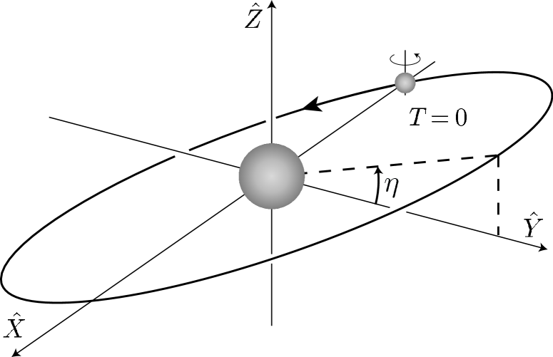
Figure 1: Orbit of Earth in Sun-based frame

In the Sun-based frame, the spatial origin coincides with the center of the Sun. The unit vector $\hat{Z}$ is parallel to the Earth’s rotational axis, $\hat{X}$ points to the vernal equinox on the celestial sphere, and $\hat{Y}$ completes the right-handed system. The time $T$ is measured by a clock fixed at the origin, with $T=0$ chosen as the vernal equinox in the year 2000. Note that the vectors $\hat{X}$, $\hat{Y}$ lie in the Earth’s equatorial plane, which itself is at an angle of $\eta\approx 23^{\circ}$ to the Earth’s orbital plane. Note also that the Earth is on the negative $X$ axis at time $T=0$. See Fig. 1.

For a space-based experiment, the time variation of the clock frequency is determined by the satellite orbital and rotational motions. To extract the leading-order effects relevant for experiments on the Earth and on the ISS, it suffices to approximate the orbits as circles. Any ellipticity introduces time dependence at higher harmonics of orbital frequencies, suppressed by even powers of the orbit eccentricity $\varepsilon^{2}$. For example, a time dependence proportional to $\cos\omega t$ under the circular-orbit approximation generates an order-$\varepsilon^{2}$ dependence $\sim\varepsilon^{2}\cos 3\omega t$ for an elliptical orbit. These harmonics appear only at subleading order for any quantity that they modify. For present purposes, the circular approximation is reasonable because $\varepsilon_{\oplus}^{2}\simeq 0.029$ for the Earth’s orbit and $\varepsilon_{s}^{2}\simeq 0.032$ for the ISS orbit. However, dedicated satellite missions could have strongly elliptical orbits, in which case the higher harmonics would be of interest.

Under the circular approximation, the parameters of the Earth’s orbit are the mean orbital radius $R_{\oplus}$ and the mean orbital angular frequency $\Omega_{\oplus}$. The mean Earth orbital speed is $\beta_{\oplus}=R_{\oplus}\Omega_{\oplus}$. The parameters for a circular satellite orbit around the Earth are taken as the mean orbital radius $r_{s}$, the mean satellite orbital angular frequency $\omega_{s}$, the angle $\zeta$ between the Earth’s rotation axis $\hat{Z}$ and the satellite orbital axis, the azimuthal angle $\alpha$ between the satellite and the Earth orbital planes, and a conveniently chosen reference time $T_{0}$ at which the satellite crosses the equatorial plane on an ascending orbit. See Figure 2. It is also useful to introduce the satellite time measured in the Sun-based frame, $T_{s}=T-T_{0}$. Note that the mean satellite speed with respect to the Earth’s center is $\beta_{s}=r_{s}\omega_{s}$. For special limiting orbits, $\omega_{s}$ reduces to the usual sidereal frequency fn3 . Note also that various perturbations typically cause $\alpha$ to precess.

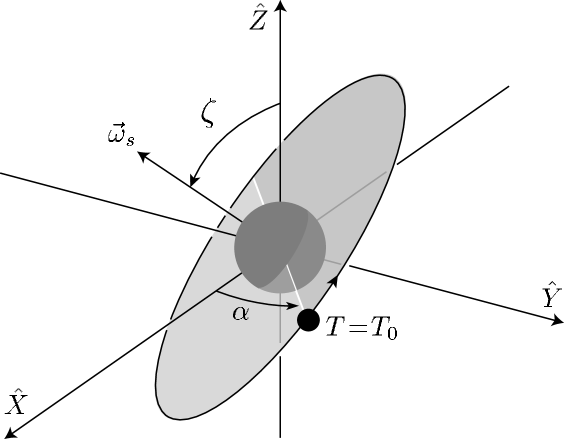
Figure 2: Parameters for definition of satellite orbit. To simplify the presentation, Earth is pictured as if it were translated to the Sun-frame coordinate origin.

	$T_{s}$	$\tilde{b}_{X}$		$\tilde{b}_{T}$					$\tilde{d}_{XY}$		$\tilde{d}_{X}$				$\tilde{g}_{-}$	$\tilde{g}_{XY}$	$\tilde{g}_{ZX}$	$\tilde{g}_{XZ}$	$\tilde{g}_{DX}$			$\tilde{c}_{X}$	$\tilde{c}_{-}$	$\tilde{c}_{TX}$
	dep.	$\tilde{b}_{Y}$	$\tilde{b}_{Z}$	$\tilde{g}_{T}$	$\tilde{d}_{+}$	$\tilde{d}_{-}$	$\tilde{d}_{Q}$	$\tilde{H}_{JT}$	$\tilde{d}_{YZ}$	$\tilde{d}_{ZX}$	$\tilde{d}_{Y}$	$\tilde{d}_{Z}$	$\tilde{g}_{c}$	$\tilde{g}_{Q}$	$\tilde{g}_{TJ}$	$\tilde{g}_{YX}$	$\tilde{g}_{ZY}$	$\tilde{g}_{YZ}$	$\tilde{g}_{DY}$	$\tilde{g}_{DZ}$	$\tilde{c}_{Q}$	$\tilde{c}_{Y}$	$\tilde{c}_{Z}$	$\tilde{c}_{TY}$	$\tilde{c}_{TZ}$
$\tilde{b}_{3}$	$\cos{\omega_{s}T_{s}}$	1	1	$\beta_{\oplus}$	$\beta_{\oplus}$	$\beta_{\oplus}$	$\beta_{\oplus}$	$\beta_{\oplus}$	$\beta_{\oplus}$	$\beta_{\oplus}$	-	-	$\beta_{\oplus}$	-	-	-	-	-	-	-	-	-	-	-	-
	$\sin{\omega_{s}T_{s}}$	1	-	$\beta_{\oplus}$	$\beta_{\oplus}$	$\beta_{\oplus}$	$\beta_{\oplus}$	$\beta_{\oplus}$	$\beta_{\oplus}$	-	-	-	$\beta_{\oplus}$	-	-	-	-	-	-	-	-	-	-	-	-
	$\cos{2\omega_{s}T_{s}}$	-	-	$\beta_{s}$	-	$\beta_{s}$	$\beta_{s}$	-	$\beta_{s}$	$\beta_{s}$	-	-	$\beta_{s}$	-	-	-	-	-	-	-	-	-	-	-	-
	$\sin{2\omega_{s}T_{s}}$	-	-	$\beta_{s}$	-	$\beta_{s}$	-	-	$\beta_{s}$	$\beta_{s}$	-	-	$\beta_{s}$	-	-	-	-	-	-	-	-	-	-	-	-
	const.	-	-	$\beta_{s}$	$\beta_{s}$	$\beta_{s}$	$\beta_{s}$	-	$\beta_{s}$	$\beta_{s}$	-	-	$\beta_{s}$	-	-	-	-	-	-	-	-	-	-	-	-
$\tilde{d}_{3}$	$\cos{\omega_{s}T_{s}}$	-	-	$\beta_{\oplus}$	$\beta_{\oplus}$	$\beta_{\oplus}$	$\beta_{\oplus}$	$\beta_{\oplus}$	$\beta_{\oplus}$	$\beta_{\oplus}$	1	1	-	-	-	$\beta_{\oplus}$	$\beta_{\oplus}$	$\beta_{\oplus}$	-	-	-	-	-	-	-
	$\sin{\omega_{s}T_{s}}$	-	-	$\beta_{\oplus}$	$\beta_{\oplus}$	$\beta_{\oplus}$	$\beta_{\oplus}$	$\beta_{\oplus}$	$\beta_{\oplus}$	$\beta_{\oplus}$	1	-	-	-	-	$\beta_{\oplus}$	$\beta_{\oplus}$	$\beta_{\oplus}$	-	-	-	-	-	-	-
	$\cos{2\omega_{s}T_{s}}$	-	-	$\beta_{s}$	-	$\beta_{s}$	$\beta_{s}$	-	$\beta_{s}$	$\beta_{s}$	-	-	-	-	-	$\beta_{s}$	$\beta_{s}$	$\beta_{s}$	-	-	-	-	-	-	-
	$\sin{2\omega_{s}T_{s}}$	-	-	-	-	$\beta_{s}$	-	-	$\beta_{s}$	$\beta_{s}$	-	-	-	-	-	$\beta_{s}$	$\beta_{s}$	$\beta_{s}$	-	-	-	-	-	-	-
	const.	-	-	$\beta_{s}$	$\beta_{s}$	$\beta_{s}$	$\beta_{s}$	-	$\beta_{s}$	$\beta_{s}$	-	-	-	-	-	$\beta_{s}$	$\beta_{s}$	$\beta_{s}$	-	-	-	-	-	-	-
$\tilde{g}_{d}$	$\cos{\omega_{s}T_{s}}$	-	-	$\beta_{\oplus}$	-	-	-	-	-	-	-	-	$\beta_{\oplus}$	-	-	$\beta_{\oplus}$	$\beta_{\oplus}$	$\beta_{\oplus}$	1	1	-	-	-	-	-
	$\sin{\omega_{s}T_{s}}$	-	-	$\beta_{\oplus}$	-	-	-	-	-	-	-	-	$\beta_{\oplus}$	-	-	-	$\beta_{\oplus}$	$\beta_{\oplus}$	1	-	-	-	-	-	-
	$\cos{2\omega_{s}T_{s}}$	-	-	$\beta_{s}$	-	-	-	-	-	-	-	-	$\beta_{s}$	-	-	$\beta_{s}$	$\beta_{s}$	$\beta_{s}$	-	-	-	-	-	-	-
	$\sin{2\omega_{s}T_{s}}$	-	-	$\beta_{s}$	-	-	-	-	-	-	-	-	$\beta_{s}$	-	-	$\beta_{s}$	$\beta_{s}$	$\beta_{s}$	-	-	-	-	-	-	-
	const.	-	-	$\beta_{s}$	-	-	-	-	-	-	-	-	$\beta_{s}$	-	-	$\beta_{s}$	$\beta_{s}$	$\beta_{s}$	-	-	-	-	-	-	-
$\tilde{c}_{q}$	$\cos{\omega_{s}T_{s}}$	-	-	-	-	-	-	-	-	-	-	-	-	-	-	-	-	-	-	-	-	-	-	$\beta_{s}$	$\beta_{s}$
	$\sin{\omega_{s}T_{s}}$	-	-	-	-	-	-	-	-	-	-	-	-	-	-	-	-	-	-	-	-	-	-	$\beta_{s}$	-
	$\cos{2\omega_{s}T_{s}}$	-	-	-	-	-	-	-	-	-	-	-	-	-	-	-	-	-	-	-	1	1	1	$\beta_{\oplus}$	$\beta_{\oplus}$
	$\sin{2\omega_{s}T_{s}}$	-	-	-	-	-	-	-	-	-	-	-	-	-	-	-	-	-	-	-	-	1	1	$\beta_{\oplus}$	$\beta_{\oplus}$
	const.	-	-	-	-	-	-	-	-	-	-	-	-	-	-	-	-	-	-	-	1	1	1	$\beta_{\oplus}$	$\beta_{\oplus}$
$\tilde{g}_{q}$	$\cos{\omega_{s}T_{s}}$	-	-	-	-	-	-	-	-	-	-	-	-	-	-	$\beta_{s}$	$\beta_{s}$	$\beta_{s}$	-	-	-	-	-	-	-
	$\sin{\omega_{s}T_{s}}$	-	-	-	-	-	-	-	-	-	-	-	-	-	-	$\beta_{s}$	-	$\beta_{s}$	-	-	-	-	-	-	-
	$\cos{2\omega_{s}T_{s}}$	-	-	$\beta_{\oplus}$	-	-	-	-	-	-	-	-	$\beta_{\oplus}$	1	1	$\beta_{\oplus}$	$\beta_{\oplus}$	$\beta_{\oplus}$	-	-	-	-	-	-	-
	$\sin{2\omega_{s}T_{s}}$	-	-	$\beta_{\oplus}$	-	-	-	-	-	-	-	-	$\beta_{\oplus}$	-	1	$\beta_{\oplus}$	$\beta_{\oplus}$	$\beta_{\oplus}$	-	-	-	-	-	-	-
	const.	-	-	$\beta_{\oplus}$	-	-	-	-	-	-	-	-	$\beta_{\oplus}$	1	1	$\beta_{\oplus}$	$\beta_{\oplus}$	$\beta_{\oplus}$	-	-	-	-	-	-	-

Table 1: Dependence of clock-frame coefficients on satellite time $T_{s}$ and on Sun-frame tilde coefficients.

The rotational motion of the satellite is specified by giving its orientation as a function of time. Two flight modes are commonly considered ISS , often denoted XVV and XPOP. In XPOP mode, the satellite orientation is fixed in the Sun-based frame as it orbits the Earth. All clock signals from Lorentz violation are due to boosts associated with the satellite orbital motion in this frame, so they are suppressed by at least one power of $\beta_{\oplus}$ or $\beta_{s}$. In contrast, for the XVV (“airplane”) mode, the satellite rotates once in the Sun frame each time it orbits the Earth, so its orientation is fixed relative to the instantaneous tangent to the satellite’s circular orbit about the Earth. Clock signals in this mode are due to both rotations and boosts, so they are sensitive to a wide variety of Lorentz-violating effects. In what follows, we focus on the XVV mode.

In the space-based laboratory, the coordinate system is defined as follows spaceexpt ; km . The 3 axis is taken along the satellite velocity with respect to the Earth. The 1 axis is chosen to point towards the center of Earth. The 2 axis completes the right-handed system and is oriented along the satellite orbital angular momentum with respect to the Earth. The clock orientation in the laboratory is typically determined by an applied magnetic field, which establishes a quantization axis. For definiteness, we take the quantization axis as the 3 axis in this work. Other choices of quantization axis can readily be calculated by our methods km . Although the detailed time-varying signals are different, no additional sensitivities to Lorentz violation are obtained with other choices.

Combining information from the above frame, mode, and orientation choices permits the construction of the explicit transformation ${\cal T}$ between the Sun-based and laboratory frames. Acting on vector components, the transformation can be regarded as a matrix with components ${{\cal T}_{\mu}}^{\Xi}$ that depend on various velocities, frequencies, angles, and Sun-frame times. The derivation of this matrix is provided in Appendix A. With this matrix, the explicit time dependence of the quantities $\tilde{b}_{3}^{w}$, $\tilde{d}_{3}^{w}$, $\tilde{g}_{d}^{w}$, $\tilde{c}_{q}^{w}$, $\tilde{g}_{q}^{w}$, can readily be calculated in terms of the Sun-frame coefficients $a_{\Xi}^{w}$, $b_{\Xi}^{w}$, $c_{\Xi\Pi}^{w}$, $d_{\Xi\Pi}^{w}$, $e_{\Xi}^{w}$, $f_{\Xi}^{w}$, $g_{\Xi\Pi\Sigma}^{w}$, $H_{\Xi\Pi}^{w}$ appearing in the fermion sector of the SME, where $\Xi$, $\Pi$, $\Sigma$ are indices spanning the Sun-frame coordinates $(T,X,Y,Z)$. For example, $b_{3}={{\cal T}_{3}}^{\Xi}b_{\Xi}$, and $d_{03}={{\cal T}_{0}}^{\Xi}{{\cal T}_{3}}^{\Pi}d_{\Xi\Pi}$.

Due to the relatively involved spiral nature of the satellite trajectory as observed in the Sun-frame, the resulting explicit expressions for the quantities $\tilde{b}_{3}^{w}$, $\tilde{d}_{3}^{w}$, $\tilde{g}_{d}^{w}$, $\tilde{c}_{q}^{w}$, $\tilde{g}_{q}^{w}$, are somewhat lengthy. It turns out to be simpler and natural to express these in terms of certain special “tilde” combinations of Sun-frame coefficients for Lorentz violation fn4 . These combinations are listed in Appendix B. For each of the three species, 40 independent Sun-frame tilde coefficients play a role at the level of zeroth- and first-order relativistic effects considered here. There are therefore 120 linearly independent degrees of freedom that can be probed in clock-comparison experiments with ordinary matter at this relativistic order. Note that for each species the SME coefficients $a_{\mu}$, $b_{\mu}$, $c_{\mu\nu}$, $d_{\mu\nu}$, $e_{\mu}$, $f_{\mu}$, $g_{\lambda\mu\nu}$, $H_{\mu\nu}$ contain a total of 44 physically observable coefficients at leading order in Lorentz violation once unphysical field redefinitions have been fixed ck ; cm ; bek , so four additional Sun-frame tilde coefficients are required to form a complete set of physical observables for clock-comparison experiments. However, these can appear at most as subleading-order relativistic effects with signals suppressed by two powers of the velocities $\beta_{\oplus}$, $\beta_{s}$ and are therefore not considered in this work.

The resulting expressions for $\tilde{b}_{3}^{w}$, $\tilde{d}_{3}^{w}$, $\tilde{g}_{d}^{w}$, $\tilde{c}_{q}^{w}$, $\tilde{g}_{q}^{w}$, are given in Appendix C. Each equation is a linear combination of Sun-frame tilde coefficients. The multiplicative factors are constants of order 1, sines or cosines of the angles $\alpha$, $2\alpha$, $\zeta$, $2\zeta$, $\eta$, and time oscillations involving sines or cosines of $\omega_{s}T_{s}$, $2\omega_{s}T_{s}$, $\Omega_{\oplus}T$. Note that the terms involving $\Omega_{\oplus}$ vary relatively slowly with time because $\omega_{s}\gg\Omega_{\oplus}$. The same is true of any precession time dependence in the orbital angle $\alpha$. Note also that the usual nonrelativistic dependence kla is recovered in the nonrelativistic limit $\beta_{\oplus}\rightarrow 0,\beta_{s}\rightarrow 0$.

Insight into the content of these equations can be obtained by separating each according to distinct satellite-frequency dependences and classifying the resulting terms according to velocity dependence. Since $\beta_{\oplus}\simeq 10^{-4}$ for the Earth and $\beta_{s}\simeq 10^{-5}$ for the ISS, the terms linear in the velocities are suppressed relative to the zeroth-order ones. Table 1 lists the decomposition of the equations in Appendix C in accordance with this scheme. As an explicit example, consider the variation of $\tilde{c}_{q}$ with the fundamental satellite frequency $\omega_{s}$. This is contained in the full expression for $\tilde{c}_{q}$ presented in Eq. (32), from which the relevant terms can be extracted and rearranged in the form

$$\tilde{c}_{q} \supset \beta_{s}(2s_{\alpha}c_{\zeta}\tilde{c}_{TX}-2c_{\alpha}c_{\zeta}\tilde{c}_{TY}-2s_{\zeta}\tilde{c}_{TZ})\cos{\omega_{s}T_{s}}$$ (11)

$$+\beta_{s}(2c_{\alpha}\tilde{c}_{TX}+2s_{\alpha}\tilde{c}_{TY})\sin{\omega_{s}T_{s}}.$$

Table 1 separates the sine and cosine dependence of this expression and lists factors of $\beta_{s}$ in the appropriate columns for the coefficients $\tilde{c}_{TX}$, $\tilde{c}_{TY}$, $\tilde{c}_{TZ}$. In general, this type of structural information about the equations in Appendix C is useful in establishing sensitivities for different experiments.

IV Signals and sensitivities

	${}^{133}{\rm Cs}$	${}^{133}{\rm Cs}$	${}^{133}{\rm Cs}$	${}^{133}{\rm Cs}$	${}^{133}{\rm Cs}$	${}^{87}{\rm Rb}$	${}^{87}{\rm Rb}$	${}^{87}{\rm Rb}$	${}^{87}{\rm Rb}$	${}^{87}{\rm Rb}$	${}^{1}{\rm H}$
transition	$(4,0)$	$(4,1)$	$(4,-1)$	$(4,0)$	$(4,0)$	$(2,1)$	$(2,-1)$	$(2,1)$	$(2,0)$	$(2,0)$	$(1,1)$
	$\to(3,0)$	$\to(3,1)$	$\to(3,-1)$	$\to(3,1)$	$\to(3,-1)$	$\to(1,1)$	$\to(1,-1)$	$\to(1,0)$	$\to(1,1)$	$\to(1,-1)$	$\to(1,0)$
$I$	$7/2$	$7/2$	$7/2$	$7/2$	$7/2$	$3/2$	$3/2$	$3/2$	$3/2$	$3/2$	$1/2$
$Z$	$55$	$55$	$55$	$55$	$55$	$37$	$37$	$37$	$37$	$37$	$1$
$N$	$78$	$78$	$78$	$78$	$78$	$50$	$50$	$50$	$50$	$50$	$0$
Schmidt	$g_{7/2}$	$g_{7/2}$	$g_{7/2}$	$g_{7/2}$	$g_{7/2}$	$p_{3/2}$	$p_{3/2}$	$p_{3/2}$	$p_{3/2}$	$p_{3/2}$	$s_{1/2}$
nucleon
$e^{-}$ state	$s_{1/2}$	$s_{1/2}$	$s_{1/2}$	$s_{1/2}$	$s_{1/2}$	$s_{1/2}$	$s_{1/2}$	$s_{1/2}$	$s_{1/2}$	$s_{1/2}$	$s_{1/2}$
$\beta_{p}$	$[{{7}\over{9}}]$	$[{{7}\over{9}}]$	$[{{7}\over{9}}]$	$[{{7}\over{9}}]$	$[{{7}\over{9}}]$	$[-1]$	$[-1]$	$[-1]$	$[-1]$	$[-1]$	$-1$
$\gamma_{p}$	$[-{{1}\over{9}}K_{p}]$	$[-{{1}\over{9}}K_{p}]$	$[-{{1}\over{9}}K_{p}]$	$[-{{1}\over{9}}K_{p}]$	$[-{{1}\over{9}}K_{p}]$	$[-{{1}\over{15}}K_{p}]$	$[-{{1}\over{15}}K_{p}]$	$[-{{1}\over{15}}K_{p}]$	$[-{{1}\over{15}}K_{p}]$	$[-{{1}\over{15}}K_{p}]$	$0$
$\delta_{p}$	$[-{{7}\over{33}}K_{p}]$	$[-{{7}\over{33}}K_{p}]$	$[-{{7}\over{33}}K_{p}]$	$[-{{7}\over{33}}K_{p}]$	$[-{{7}\over{33}}K_{p}]$	$[{{1}\over{5}}K_{p}]$	$[{{1}\over{5}}K_{p}]$	$[{{1}\over{5}}K_{p}]$	$[{{1}\over{5}}K_{p}]$	$[{{1}\over{5}}K_{p}]$	${{1}\over{3}}K_{p}$
$\kappa_{p}$	$[{{28}\over{99}}K_{p}]$	$[{{28}\over{99}}K_{p}]$	$[{{28}\over{99}}K_{p}]$	$[{{28}\over{99}}K_{p}]$	$[{{28}\over{99}}K_{p}]$	$[-{{2}\over{5}}K_{p}]$	$[-{{2}\over{5}}K_{p}]$	$[-{{2}\over{5}}K_{p}]$	$[-{{2}\over{5}}K_{p}]$	$[-{{2}\over{5}}K_{p}]$	$-{{1}\over{3}}K_{p}$
$\lambda_{p}$	$[0]$	$[0]$	$[0]$	$[0]$	$[0]$	$[0]$	$[0]$	$[0]$	$[0]$	$[0]$	$0$
$\beta_{e}$	$-1$	$-1$	$-1$	$-1$	$-1$	$-1$	$-1$	$-1$	$-1$	$-1$	$-1$
$\gamma_{e}$	$0$	$0$	$0$	$0$	$0$	$0$	$0$	$0$	$0$	$0$	$0$
$\delta_{e}$	${{1}\over{3}}K_{e}$	${{1}\over{3}}K_{e}$	${{1}\over{3}}K_{e}$	${{1}\over{3}}K_{e}$	${{1}\over{3}}K_{e}$	${{1}\over{3}}K_{e}$	${{1}\over{3}}K_{e}$	${{1}\over{3}}K_{e}$	${{1}\over{3}}K_{e}$	${{1}\over{3}}K_{e}$	${{1}\over{3}}K_{e}$
$\kappa_{e}$	$-{{1}\over{3}}K_{e}$	$-{{1}\over{3}}K_{e}$	$-{{1}\over{3}}K_{e}$	$-{{1}\over{3}}K_{e}$	$-{{1}\over{3}}K_{e}$	$-{{1}\over{3}}K_{e}$	$-{{1}\over{3}}K_{e}$	$-{{1}\over{3}}K_{e}$	$-{{1}\over{3}}K_{e}$	$-{{1}\over{3}}K_{e}$	$-{{1}\over{3}}K_{e}$
$\lambda_{e}$	$0$	$0$	$0$	$0$	$0$	$0$	$0$	$0$	$0$	$0$	$0$
$s_{1}^{p}$	$0$	$-1/14$	$1/14$	$-9/28$	$9/28$	$-1/3$	$1/3$	$1/2$	$-5/6$	$5/6$	$1$
$s_{2}^{p}$	$0$	$-1/14$	$-1/14$	$-5/28$	$-5/28$	$-1$	$-1$	$1/2$	$-3/2$	$-3/2$	$-$
$s_{1}^{e}$	$0$	$1/2$	$-1/2$	$1/4$	$-1/4$	$1$	$-1$	$1/2$	$1/2$	$-1/2$	$1$

Table 2: Parameters for transition frequencies for experiments with Cs, Rb, and H clocks.

At this stage, we can use the time dependence of the quantities $\tilde{b}_{3}^{w}$, $\tilde{d}_{3}^{w}$, $\tilde{g}_{d}^{w}$, $\tilde{c}_{q}^{w}$, $\tilde{g}_{q}^{w}$, derived in the previous section to study the signals in clock-comparison experiments involving various atomic transitions. We focus specifically on transitions $(F,m_{F})\rightarrow({F}^{\prime},{m}^{\prime}_{F})$ in species scheduled for flight on the ISS: ${}^{87}{\rm Rb}$, ${}^{133}{\rm Cs}$, and H. These have an even number of neutrons and total electronic angular momentum $J=1/2$. The generalization of our results to nuclei with an odd number of neutrons is straightforward.

The Lorentz-violating contribution $\delta\omega$ to the frequency of the transition $(F,m_{F})\rightarrow({F}^{\prime},{m}^{\prime}_{F})$ is given by Eqs. (2) and (3). With the above assumptions, this frequency shift can be expressed as:

$$\hskip-15.0pt\delta\omega = s_{1}^{p}\left[\beta_{p}(l_{j})\tilde{b}_{3}^{p}+\delta_{p}(l_{j})\tilde{d}_{3}^{p}+\kappa_{p}(l_{j})\tilde{g}_{d}^{p}\right]$$ (12)

$$+s_{2}^{p}\left[\gamma_{p}(l_{j})\tilde{c}_{q}^{p}+\lambda_{p}(l_{j})\tilde{g}_{q}^{p}\right]$$

$$+s_{1}^{e}\left[\beta_{e}(0_{1/2})\tilde{b}_{3}^{e}+\delta_{e}(0_{1/2})\tilde{d}_{3}^{e}+\kappa_{e}(0_{1/2})\tilde{g}_{d}^{e}\right].$$

In this equation, each $l_{j}$ refers to the Schmidt nucleon. Except for the quantities $s_{j}^{w}$ outside the brackets, all variables in Eq. (12) are those appearing in Eq. (3). The specific values of the quantities $\beta_{w}$, $\gamma_{w}$, $\delta_{w}$, $\kappa_{w}$, $\lambda_{w}$ are given as Eqs. (11) and (12) of Ref. kla . The values of $s_{j}^{w}$ depend on the transition, and formulæ for them are given below. Note that similar equations valid for more general atoms would also involve $s_{2}^{e}$, $s_{1}^{n}$, and $s_{2}^{n}$ terms.

The expressions for the $s_{j}^{w}$ can be classified according to the possible values of $F$ and ${F}^{\prime}$. There are four cases of interest. For each case, we give the expressions first in terms of combinations of Clebsch-Gordan coefficients and angular-momentum quantum numbers, and then directly in terms of $m_{F}$ and ${m}^{\prime}_{F}$. In all cases, we define $\Delta m_{F}:=m_{F}-{m}^{\prime}_{F}$ and $\Delta m_{F}^{2}:=m_{F}^{2}-({m}^{\prime}_{F})^{2}$.

The first case has $F={F}^{\prime}=I+{\textstyle{1\over 2}}$, for which we obtain

$$s_{1}^{p} =\widehat{m}_{F}-{\widehat{m}_{F}}^{\prime} =\left[{\textstyle{{2}\over{2I+1}}}\right]\Delta m_{F},$$

$$s_{2}^{p} =\widetilde{m}_{F}-{\widetilde{m}_{F}}^{\prime} =\left[{\textstyle{{3}\over{I(2I+1)}}}\right]\Delta m_{F}^{2},$$

$$s_{1}^{e} =\widehat{m}_{F}-{\widehat{m}_{F}}^{\prime} =\left[{\textstyle{{2}\over{2I+1}}}\right]\Delta m_{F}.$$ (13)

The second case has $F={F}^{\prime}=I-{\textstyle{1\over 2}}$, and we find

$$s_{1}^{p}= (\widehat{m}_{F}-{\widehat{m}_{F}}^{\prime}){\textstyle{{(I+1)(2I-1)}\over{I(2I+1)}}} =\left[{\textstyle{{2I+2}\over{I(2I+1)}}}\right]\Delta m_{F},$$

$$s_{2}^{p}= (\widetilde{m}_{F}-{\widetilde{m}_{F}}^{\prime}){\textstyle{{(I-1)(2I+3)}\over{I(2I+1)}}} =\left[{\textstyle{{3(2I+3)}\over{I(2I+1)(2I-1)}}}\right]\Delta m_{F}^{2},$$

$$s_{1}^{e}= (\widehat{m}_{F}-{\widehat{m}_{F}}^{\prime}){\textstyle{{1-2I}\over{1+2I}}} =\left[{\textstyle{{-2}\over{2I+1}}}\right]\Delta m_{F}.$$ (14)

The third case has $F=I+{\textstyle{1\over 2}},{F}^{\prime}=I-{\textstyle{1\over 2}}$, giving

$$s_{1}^{p} = \widehat{m}_{F}-{\textstyle{{(I+1)(2I-1)}\over{I(2I+1)}}}{\widehat{m}_{F}}^{\prime}$$

$$= \left[{\textstyle{{2}\over{2I+1}}}\right]\Delta m_{F}-\left[{\textstyle{{2}\over{I(2I+1)}}}\right]{m}^{\prime}_{F},$$

$$s_{2}^{p} = \widetilde{m}_{F}-{\textstyle{{(I-1)(2I+3)}\over{I(2I+1)}}}{\widetilde{m}_{F}}^{\prime}$$

$$= \left[{\textstyle{{3}\over{I(2I+1)}}}\right]\Delta m_{F}^{2}-\left[{\textstyle{{12}\over{I(2I+1)(2I-1)}}}\right]({m}^{\prime}_{F})^{2},$$

$$s_{1}^{e} = \widehat{m}_{F}-{\textstyle{{1-2I}\over{1+2I}}}{\widehat{m}_{F}}^{\prime}$$ (15)

$$= \left[{\textstyle{{2}\over{2I+1}}}\right]\Delta m_{F}+\left[{\textstyle{{4}\over{2I+1}}}\right]{m}^{\prime}_{F}.$$

The final case has $F=I-{\textstyle{1\over 2}},{F}^{\prime}=I+{\textstyle{1\over 2}}$, for which

$$s_{1}^{p} = {\textstyle{{(I+1)(2I-1)}\over{I(2I+1)}}}\widehat{m}_{F}-{\widehat{m}_{F}}^{\prime}$$

$$= \left[{\textstyle{{2}\over{2I+1}}}\right]\Delta m_{F}+\left[{\textstyle{{2}\over{I(2I+1)}}}\right]m_{F},$$

$$s_{2}^{p} = {\textstyle{{(I-1)(2I+3)}\over{I(2I+1)}}}\widetilde{m}_{F}-{\widetilde{m}_{F}}^{\prime}$$

$$= \left[{\textstyle{{3}\over{I(2I+1)}}}\right]\Delta m_{F}^{2}+\left[{\textstyle{{12}\over{I(2I+1)(2I-1)}}}\right]m_{F}^{2},$$

$$s_{1}^{e} = {\textstyle{{1-2I}\over{1+2I}}}\widehat{m}_{F}-{\widehat{m}_{F}}^{\prime}$$ (16)

$$= \left[{\textstyle{{2}\over{2I+1}}}\right]\Delta m_{F}-\left[{\textstyle{{4}\over{2I+1}}}\right]m_{F}.$$

Various results can be obtained from these expressions and Eq. (12). For example, it follows directly that a nonzero signal occurs for all $\Delta F=\pm 1$, $\Delta m_{F}=0$ transitions except for the special case $m_{F}={m}^{\prime}_{F}=0$. This demonstrates that the standard clock transitions are insensitive to Lorentz-violating effects, in agreement with previous results kla . Useful special cases of immediate relevance to experiments on the ISS can also be extracted. Thus, for a ${}^{133}{\rm Cs}$ clock with $I={\textstyle{{7}\over{2}}}$, $F=4\rightarrow 3$, we find:

$$s_{1}^{p} = {\textstyle{{1}\over{4}}}\Delta m_{F}-{\textstyle{{1}\over{14}}}{m}^{\prime}_{F},$$

$$s_{2}^{p} = {\textstyle{{3}\over{28}}}\Delta m_{F}^{2}-{\textstyle{{1}\over{14}}}({m}^{\prime}_{F})^{2},$$

$$s_{1}^{e} = {\textstyle{{1}\over{4}}}\Delta m_{F}+{\textstyle{{1}\over{2}}}{m}^{\prime}_{F}.$$ (17)

Similarly, for a ${}^{87}{\rm Rb}$ clock with $I={\textstyle{{3}\over{2}}}$, $F=2\rightarrow 1$, we obtain:

$$s_{1}^{p} = {\textstyle{{1}\over{2}}}\Delta m_{F}-{\textstyle{{1}\over{3}}}{m}^{\prime}_{F},$$

$$s_{2}^{p} = {\textstyle{{1}\over{2}}}\Delta m_{F}^{2}-({m}^{\prime}_{F})^{2},$$

$$s_{1}^{e} = {\textstyle{{1}\over{2}}}\Delta m_{F}+{m}^{\prime}_{F}.$$ (18)

For an H clock or maser, $s_{1}^{e}=s_{1}^{p}=1$. However, $s_{2}^{p}$ is irrelevant: the proton is in an $I=1/2$ state, so there is no quadrupole effect and the quantities $\gamma_{p}$ and $\lambda_{p}$ vanish.

Table 2 summarizes some useful results for species scheduled for flight on the ISS. The first few rows of this table identify the transition and list various properties of the species involved. The nuclear spin is $I$, the proton number is $Z$, and the neutron number is $N$. The following entry fixes the proton determining the ground-state properties of the nucleus following the nuclear Schmidt model sch , together with its associated orbital and total angular momentum. The electronic configuration is also given. Ten rows list the relevant parameters $\beta_{w}$, $\delta_{w}$, $\kappa_{w}$, $\gamma_{w}$, $\lambda_{w}$, with values in brackets obtained under the assumptions of the Schmidt model. We define $K_{p}=\langle{p^{2}}\rangle/m_{p}^{2}$, which can be regarded as twice the kinetic energy per mass of the Schmidt-model proton, and define $K_{e}$ similarly for the valence electron. An estimate gives $K_{p}\simeq 10^{-2}$ for all species except ¹H, for which $K_{p}\simeq 10^{-11}$, and $K_{e}\simeq 10^{-5}$. Finally, the numerical values of the $s_{j}^{w}$ are listed. Where these are nonzero, a clock-comparison experiment with the specified transition is sensitive to Lorentz violation.

At this stage, enough information is at hand to extract estimated experimental sensitivities. Suppose the results of an experiment measuring the modified frequency difference $\omega^{\sharp}$ of Eq. (4) are fitted to the form

$$\omega^{\sharp} = \mbox{constant}+2\pi\varepsilon_{1,X}\cos{\omega_{s}T_{s}}+2\pi\varepsilon_{1,Y}\sin{\omega_{s}T_{s}}$$ (19)

$$+2\pi\varepsilon_{2,X}\cos{2\omega_{s}T_{s}}+2\pi\varepsilon_{2,Y}\sin{2\omega_{s}T_{s}}.$$

Nonzero values of any of the $\varepsilon_{a,J}$ indicate Lorentz violation. Denote by $\varepsilon_{a}$ the minimum of $\{|\varepsilon_{a,X}|,|\varepsilon_{a,Y}|\}$. Then, combining the theoretical analysis above yields the following predicted dependence of $\varepsilon_{a}$ on coefficients for Lorentz violation, atomic and nuclear parameters, and geometrical factors:

$$2\pi\varepsilon_{1} = \bigg{|}\sum_{w}\bigg{[}(s_{1}^{wA}\beta_{w}^{A}-vs_{1}^{wB}\beta_{w}^{B})(\tilde{b}_{J}^{w})+\beta_{\oplus}\big{[}s_{1}^{wA}(\beta_{w}^{A}+\delta_{w}^{A}+\kappa_{w}^{A})-vs_{1}^{wB}(\beta_{w}^{B}+\delta_{w}^{B}+\kappa_{w}^{B})\big{]}(\tilde{b}_{T}^{w},\tilde{g}_{T}^{w})$$ (20)

$$+\beta_{\oplus}\big{[}s_{1}^{wA}(\beta_{w}^{A}+\delta_{w}^{A})-vs_{1}^{wB}(\beta_{w}^{B}+\delta_{w}^{B})\big{]}(\tilde{d}_{\pm}^{w},\tilde{d}_{Q}^{w},\tilde{d}_{JK}^{w},\tilde{H}_{JT}^{w})+(s_{1}^{wA}\delta_{w}^{A}-vs_{1}^{wB}\delta_{w}^{B})(\tilde{d}_{J}^{w})$$

$$+(s_{1}^{wA}\kappa_{w}^{A}-vs_{1}^{wB}\kappa_{w}^{B})(\tilde{g}_{DJ}^{w})+\big{[}\beta_{\oplus}s_{1}^{wA}(\delta_{w}^{A}+\kappa_{w}^{A})-\beta_{\oplus}vs_{1}^{wB}(\delta_{w}^{B}+\kappa_{w}^{B})+\beta_{s}(s_{2}^{wA}\lambda_{w}^{A}-vs_{2}^{wB}\lambda_{w}^{B})\big{]}(\tilde{g}_{JK}^{w})$$

$$+\beta_{\oplus}\big{[}s_{1}^{wA}(\beta_{w}^{A}+\kappa_{w}^{A})-vs_{1}^{wB}(\beta_{w}^{B}+\kappa_{w}^{B})\big{]}(\tilde{g}_{c}^{w})+\beta_{s}(s_{2}^{wA}\gamma_{w}^{A}-vs_{2}^{wB}\gamma_{w}^{B})(\tilde{c}_{TJ}^{w})\bigg{]}\bigg{|},$$

$$2\pi\varepsilon_{2} = \bigg{|}\sum_{w}\bigg{[}\big{[}\beta_{s}s_{1}^{wA}(\beta_{w}^{A}+\delta_{w}^{A}+\kappa_{w}^{A})-\beta_{s}vs_{1}^{wB}(\beta_{w}^{B}+\delta_{w}^{B}+\kappa_{w}^{B})+\beta_{\oplus}(s_{2}^{wA}\lambda_{w}^{A}-vs_{2}^{wB}\lambda_{w}^{B})\big{]}(\tilde{b}_{T}^{w},\tilde{g}_{T}^{w})$$ (21)

$$+\beta_{s}\big{[}s_{1}^{wA}(\beta_{w}^{A}+\delta_{w}^{A})-vs_{1}^{wB}(\beta_{w}^{B}+\delta_{w}^{B})\big{]}(\tilde{d}_{-}^{w},\tilde{d}_{Q}^{w},\tilde{d}_{JK}^{w})+\beta_{s}(s_{1}^{wA}\beta_{w}^{A}-vs_{1}^{wB}\beta_{w}^{B})(\tilde{H}_{JT}^{w})$$

$$+\big{[}\beta_{s}s_{1}^{wA}(\delta_{w}^{A}+\kappa_{w}^{A})-\beta_{s}vs_{1}^{wB}(\delta_{w}^{B}+\kappa_{w}^{B})+\beta_{\oplus}(s_{2}^{wA}\lambda_{w}^{A}-vs_{2}^{wB}\lambda_{w}^{B})\big{]}(\tilde{g}_{JK}^{w})$$

$$+\big{[}\beta_{s}s_{1}^{wA}(\beta_{w}^{A}+\kappa_{w}^{A})-\beta_{s}vs_{1}^{wB}(\beta_{w}^{B}+\kappa_{w}^{B})+\beta_{\oplus}(s_{2}^{wA}\lambda_{w}^{A}-vs_{2}^{wB}\lambda_{w}^{B})\big{]}(\tilde{g}_{c}^{w})+\beta_{\oplus}(s_{2}^{wA}\gamma_{w}^{A}-vs_{2}^{wB}\gamma_{w}^{B})(\tilde{c}_{TJ}^{w})$$

$$+(s_{2}^{wA}\gamma_{w}^{A}-vs_{2}^{wB}\gamma_{w}^{B})(\tilde{c}_{-}^{w},\tilde{c}_{Q}^{w},\tilde{c}_{J}^{w})+(s_{2}^{wA}\lambda_{w}^{A}-vs_{2}^{wB}\lambda_{w}^{B})(\tilde{g}_{-}^{w},\tilde{g}_{Q}^{w},\tilde{g}_{TJ}^{w})\bigg{]}\bigg{|}.$$

In these equations, superscripts $A$ and $B$ indicate quantities evaluated for transitions $A$ and $B$, respectively, and $J$ takes the values $(X,Y,Z)$. The coefficients for Lorentz violation enter as somewhat lengthy linear combinations of the type appearing in the equations of Appendix C. These explicit combinations are omitted here for brevity, being replaced instead with parentheses containing only the specific coefficients for Lorentz violation involved.

The above form of the equations is useful despite the brevity because it allows relatively straightforward consideration of sensitivities to the Sun-frame tilde coefficients for Lorentz violation. We adopt here the strategy of Ref. kla , in which numerical sensitivities are obtained within the Schmidt model under the plausible assumption that no substantial cancellations occur among contributions from different Sun-frame tilde coefficients for Lorentz violation. For example, if $\varepsilon_{1}$ is an experimental sensitivity to the time variation of $\omega^{\sharp}$, then Eq. (20) implies the experiment has sensitivity to each $|\tilde{b}_{J}^{w}|$ of $\sim 2\pi\varepsilon_{1}(s_{1}^{wA}\beta_{w}^{A}-vs_{1}^{wB}\beta_{w}^{B})^{-1}$. Similarly, the sensitivity to $|\tilde{b}_{T}^{w}|$ is $\sim 2\pi\varepsilon_{1}\beta_{\oplus}^{-1}[s_{1}^{wA}(\beta_{w}^{A}+\delta_{w}^{A}+\kappa_{w}^{A})-vs_{1}^{wB}(\beta_{w}^{B}+\delta_{w}^{B}+\kappa_{w}^{B})]^{-1}$, and so on. To obtain crude order of magnitude numerical estimates, it suffices to approximate $\beta_{s}\sim 10^{-5}$, $\beta_{\oplus}\sim 10^{-4}$, and to estimate nonzero values of the other parameters as follows: $\beta_{w}\sim 1$, $s_{a}^{w}\sim 1$ for all species; $\delta,\kappa,\gamma,\lambda\sim 10^{-2}$ for protons except for ¹H where the nonzero values are only $\delta,\kappa\sim 10^{-11}$ for the proton; and $\delta,\kappa,\gamma,\lambda\sim 10^{-5}$ for electrons. Sensitivity estimates of this type are reasonable provided the various angles $\alpha$, $2\alpha$, $\zeta$, $2\zeta$, $\eta$, $\Omega_{\oplus}T$ lie away from multiples of $\pi/4$. The orientation of the quantization axis within the satellite then makes little difference to the sensitivity. However, for any angles near a multiple of $\pi/4$, sensitivity to one or more of the Sun-frame tilde coefficients can be lost.

Coefficient	Proton	Neutron	Electron
$\tilde{b}_{X}$, $\tilde{b}_{Y}$	-27[-27]	[-31]	-27[-29]
$\tilde{b}_{Z}$	-27	-	-27[-28]
$\tilde{b}_{T}$	-23	-	-23
$\tilde{g}_{T}$	-23	-	-23
$\tilde{H}_{JT}$	-23	-	-23
$\tilde{d}_{\pm}$	-23	-	-23
$\tilde{d}_{Q}$	-23	-	-23
$\tilde{d}_{JK}$	-23	-	-23
$\tilde{d}_{X}$, $\tilde{d}_{Y}$	-25[-25]	[-29]	-22[-22]
$\tilde{d}_{Z}$	-25	-	-22
$\tilde{g}_{DX}$,$\tilde{g}_{DY}$	-25[-25]	[-29]	-22[-22]
$\tilde{g}_{DZ}$	-25	-	-22
$\tilde{g}_{JK}$	-21	-	-18
$\tilde{g}_{c}$	-23	-	-23
$\tilde{c}_{TJ}$	-20	-	-
$\tilde{c}_{-}$	-25	[-27]	-
$\tilde{c}_{Q}$	-25	-	-
$\tilde{c}_{X}$, $\tilde{c}_{Y}$	-25	[-25]	-
$\tilde{c}_{Z}$	-25	[-27]	-
$\tilde{c}_{TJ}$	-21	-	-
$\tilde{g}_{-}$	$\star$[$\star$]	[$\star$]	-
$\tilde{g}_{Q}$	$\star$	-	-
$\tilde{g}_{TX}$, $\tilde{g}_{TY}$	$\star$[$\star$]	[$\star$]	-
$\tilde{g}_{TZ}$	$\star$[$\star$]	[$\star$]	-

Table 3: Estimated sensitivity to coefficients for Lorentz violation for ISS experiments with ${}^{133}{\rm Cs}$ and ${}^{87}{\rm Rb}$ clocks. Existing bounds ccexpt ; lh ; db ; dp ; eexpt2 are shown in brackets.

Table 3 lists estimated sensitivities to Sun-frame tilde coefficients for Lorentz violation that might be attained in the planned space-based clock-comparison experiments with ${}^{133}{\rm Cs}$ and ${}^{87}{\rm Rb}$ clocks. The base-10 logarithm of the sensitivity per GeV is shown for each coefficient for Lorentz violation and for each particle species. For definiteness, the clock sensitivity has been taken as $\varepsilon_{1,2}\sim$ 50 $\mu$Hz, which is comparable to that attained in a ground-based experiment with ${}^{133}{\rm Cs}$ lh , but the results shown are readily scaled for other values of $\varepsilon_{1,2}$. A star in the table indicates a combination for which there is no sensitivity according to the nuclear Schmidt model but probable sensitivity in a more realistic nuclear model. A value in brackets indicates an existing bound from an Earth-based experiment ccexpt ; lh ; db ; dp ; eexpt2 . Given the approximations described above, some caution in interpretation of the details of this table is advisable. Nonetheless, the table provides a measure of the broad scope of space-based tests of Lorentz symmetry, and it shows that Planck-scale sensitivity for a wide spectrum of relativity tests is attainable.

Space-based experiments exploring the photon sector of the SME have been studied elsewhere km , including the SUMO experiment with superconducting microwave-cavity oscillators that is presently scheduled for flight. Experiments of this type could be profitably combined with the clock-comparison experiments discussed in the present work. For example, at the time of writing PARCS and SUMO are planned for simultaneous flight. Several configurations of interest could then be considered, including operating PARCS on a Lorentz-insensitive line as a reference for relativity tests with SUMO, or seeking $\omega_{s}$ and $2\omega_{s}$ signals in a configuration with both the atomic clock and the cavity operating in modes sensitive to Lorentz violation.

V Summary

This work has studied clock-comparison experiments on a space-based platform, with specific emphasis placed on forthcoming experiments on the International Space Station. The theoretical framework adopted is the Standard-Model Extension, which describes general Lorentz and CPT violation. The analysis yields predictions for signals at the ISS orbital and double-orbital frequencies, along with slower variations associated with the Earth orbital motion.

The formalism we have presented applies to any space-based experiment with atomic clocks and incorporates relativistic effects at first boost order. We have derived explicit expressions for the observable effects in the special cases of ${}^{133}{\rm Cs}$, ${}^{87}{\rm Rb}$, and H clocks on the ISS, which are currently planned for flight in the PARCS, ACES, and RACE missions. These results, which involve the fermion sector of the SME, complement the photon-sector analysis of Lorentz-violation sensitivity performed for the planned SUMO experiment with microwaves on the ISS.

We have obtained estimates for the attainable sensitivities with these atomic-clock missions, listed in Table 3. Numerous currently unmeasured coefficients for Lorentz violation could be studied in these experiments. The results demonstrate that experiments of this type offer potential sensitivity to violations of relativity with Planck-scale reach.

Appendix A Transformation from Sun-based to satellite frame

In this appendix, we derive the transformation matrix ${{\cal T}_{\mu}}^{\Xi}$ introduced in Sec. III that maps Sun-frame quantities to laboratory-frame ones. The transformation ${\cal T}$ can be expressed as the composition of a boost $\Lambda$ from the Sun frame to the (nonrotating) rest frame of the center of the satellite, followed by a rotation ${\cal R}$ from the (nonrotating) rest frame of the center of the satellite to the (rotating) lab frame. Each constituent transformation depends on time, and each is understood to be instantaneous. We first obtain an expression for the satellite position in the Sun frame, then use this to derive the instantaneous satellite velocity in the Sun frame, and finally combine information to construct the desired overall transformation. The conventions we adopt are those given in Refs. spaceexpt ; km .

The position $\vec{X}_{\oplus}$ of the center of the Earth in the Sun-based frame is given by

$$\vec{X}_{\oplus}=\left(\begin{array}[]{c}-R_{\oplus}\cos{\Omega_{\oplus}T}\\ -R_{\oplus}\cos{\eta}\sin{\Omega_{\oplus}T}\\ -R_{\oplus}\sin{\eta}\sin{\Omega_{\oplus}T}\end{array}\right).$$ (22)

The satellite position $\vec{X}_{s}$ in this frame is obtained by adding the position of the satellite with respect to the Earth, which gives

$$\vec{X}_{s}=\left(\begin{array}[]{c}-R_{\oplus}\cos{\Omega_{\oplus}T}+r_{s}\cos{\alpha}\cos{\omega_{s}T_{s}}-r_{s}\cos{\zeta}\sin{\alpha}\sin{\omega_{s}T_{s}}\\ -R_{\oplus}\cos{\eta}\sin{\Omega_{\oplus}T}+r_{s}\sin{\alpha}\cos{\omega_{s}T_{s}}+r_{s}\cos{\alpha}\cos{\zeta}\sin{\omega_{s}T_{s}}\\ -R_{\oplus}\sin{\eta}\sin{\Omega_{\oplus}T}+r_{s}\sin{\zeta}\sin{\omega_{s}T_{s}}\end{array}\right).$$ (23)

Disregarding rotations for the moment, the boost $\Lambda$ from the Sun-based frame to the nonrotating instantaneous satellite rest frame is determined by the velocity $\vec{V}=d\vec{X_{s}}/dT$. To lowest order in $|\vec{V}|$, this is

$$\Lambda=\left(\begin{array}[]{c|ccc}1&V_{X}&V_{Y}&V_{Z}\\ \hline\cr V_{X}&1&0&0\\ V_{Z}&0&1&0\\ V_{Z}&0&0&1\end{array}\right).$$ (24)

The required rotation ${\cal R}$ from the nonrotating instantaneous satellite rest frame to the laboratory frame on the satellite may be calculated using the velocity and acceleration of the satellite with respect to the Earth, $d(\vec{X}_{s}-\vec{X}_{\oplus})/dT\sim\hat{z}$ and $d^{2}(\vec{X}_{s}-\vec{X}_{\oplus})/dT^{2}\sim\hat{x}$, and the requirement that

$$\left(\begin{array}[]{c}\hat{x}\\ \hat{y}\\ \hat{z}\end{array}\right)={\cal R}\left(\begin{array}[]{ccc}\hat{X}\\ \hat{Y}\\ \hat{Z}\end{array}\right).$$ (25)

Given $\Lambda$ and ${\cal R}$, the overall instantaneous transformation ${\cal T}$ from the Sun-based frame to the laboratory frame can be found:

$${\cal T}=\left(\begin{array}[]{c|ccc}1&0&0&0\\ \hline\cr 0&&&\\ 0&&{\cal R}&\\ 0&&&\end{array}\right)\Lambda\quad.$$ (26)

With the approximations of Sec. III, the components ${{\cal T}_{\mu}}^{\Xi}$ of the transformation matrix (26) are found to be

$${{\cal T}_{0}}^{T} = 1,$$

$${{\cal T}_{0}}^{X} = \beta_{\oplus}s_{\Omega T}-\beta_{s}s_{\alpha}c_{\zeta}\cos{\omega_{s}T_{s}}-\beta_{s}c_{\alpha}\sin{\omega_{s}T_{s}},$$

$${{\cal T}_{0}}^{Y} = -\beta_{\oplus}c_{\eta}c_{\Omega T}+\beta_{s}c_{\alpha}c_{\zeta}\cos{\omega_{s}T_{s}}-\beta_{s}s_{\alpha}\sin{\omega_{s}T_{s}},$$

$${{\cal T}_{0}}^{Z} = -\beta_{\oplus}s_{\eta}c_{\Omega T}+\beta_{s}s_{\zeta}\cos{\omega_{s}T_{s}},$$

$${{\cal T}_{1}}^{T} = (s_{\alpha}c_{\eta}c_{\Omega T}-c_{\alpha}s_{\Omega T})\beta_{\oplus}\cos{\omega_{s}T_{s}}$$

$$\hskip-10.0pt+(c_{\alpha}c_{\zeta}c_{\eta}c_{\Omega T}+s_{\zeta}s_{\eta}c_{\Omega T}+s_{\alpha}c_{\zeta}s_{\Omega T})\beta_{\oplus}\sin{\omega_{s}T_{s}},$$

$${{\cal T}_{1}}^{X} = -c_{\alpha}\cos{\omega_{s}T_{s}}+s_{\alpha}c_{\zeta}\sin{\omega_{s}T_{s}},$$

$${{\cal T}_{1}}^{Y} = -s_{\alpha}\cos{\omega_{s}T_{s}}-c_{\alpha}c_{\zeta}\sin{\omega_{s}T_{s}},$$

$${{\cal T}_{1}}^{Z} = -s_{\zeta}\sin{\omega_{s}T_{s}},$$

$${{\cal T}_{2}}^{T} = \beta_{\oplus}c_{\alpha}s_{\zeta}c_{\eta}c_{\Omega T}-\beta_{\oplus}c_{\zeta}s_{\eta}c_{\Omega T}+\beta_{\oplus}s_{\alpha}s_{\zeta}s_{\Omega T},$$

$${{\cal T}_{2}}^{X} = s_{\alpha}s_{\zeta},$$

$${{\cal T}_{2}}^{Y} = -c_{\alpha}s_{\zeta},$$

$${{\cal T}_{2}}^{Z} = c_{\zeta},$$

$${{\cal T}_{3}}^{T} = \beta_{s}+(s_{\alpha}c_{\eta}c_{\Omega T}-c_{\alpha}s_{\Omega T})\beta_{\oplus}\sin{\omega_{s}T_{s}}$$

$$\hskip-10.0pt+(-c_{\alpha}c_{\eta}c_{\zeta}c_{\Omega T}-s_{\zeta}s_{\eta}c_{\Omega T}-s_{\alpha}c_{\zeta}s_{\Omega T})\beta_{\oplus}\cos{\omega_{s}T_{s}},$$

$${{\cal T}_{3}}^{X} = -c_{\alpha}\sin{\omega_{s}T_{s}}-s_{\alpha}c_{\zeta}\cos{\omega_{s}T_{s}},$$

$${{\cal T}_{3}}^{Y} = c_{\alpha}c_{\zeta}\cos{\omega_{s}T_{s}}-s_{\alpha}\sin{\omega_{s}T_{s}},$$

$${{\cal T}_{3}}^{Z} = s_{\zeta}\cos{\omega_{s}T_{s}}.$$ (27)

In these equations, the abbreviations $s_{x}\equiv\sin x$, $c_{x}\equiv\cos x$ and $\Omega T\equiv\Omega_{\oplus}T$ are used.

Appendix B Sun-frame coefficients

The Sun-frame tilde coefficients are defined as follows:

$$\tilde{b}_{J} = b_{J}-{\textstyle{1\over 2}}\varepsilon_{JKL}H_{KL}-m(d_{JT}-{\textstyle{1\over 2}}\varepsilon_{JKL}g_{KLT}),\qquad\tilde{b}_{T}=b_{T}+mg_{XYZ},$$

$$\tilde{g}_{T} = b_{T}-m(g_{XYZ}-g_{YZX}-g_{ZXY}),$$

$$\tilde{H}_{XT} = H_{XT}+m(d_{ZY}-g_{XTT}-g_{XYY}),\qquad\tilde{H}_{YT}=H_{YT}+m(d_{XZ}-g_{YTT}-g_{YZZ}),$$

$$\tilde{H}_{ZT} = H_{ZT}+m(d_{YX}-g_{ZTT}-g_{ZXX}),$$

$$\tilde{d}_{\pm} = m(d_{XX}\pm d_{YY}),\qquad\tilde{d}_{Q}=m(d_{XX}+d_{YY}-2d_{ZZ}-g_{YZX}-g_{ZXY}+2g_{XYZ}),$$

$$\tilde{d}_{J} = m(d_{TJ}+{\textstyle{1\over 2}}d_{JT})-{\textstyle{{1}\over{4}}}\varepsilon_{JKL}H_{KL},\qquad\tilde{d}_{YZ}=m(d_{YZ}+d_{ZY}-g_{XYY}+g_{XZZ}),$$

$$\tilde{d}_{ZX} = m(d_{ZX}+d_{XZ}-g_{YZZ}+g_{YXX}),\qquad\tilde{d}_{XY}=m(d_{XY}+d_{YX}-g_{ZXX}+g_{ZYY}),$$

$$\tilde{g}_{c} = m(g_{XYZ}-g_{ZXY}),\qquad\tilde{g}_{-}=m(g_{XTX}-g_{YTY}),\qquad\tilde{g}_{Q}=m(g_{XTX}+g_{YTY}-2g_{ZTZ}),$$

$$\tilde{g}_{TJ} = m\left|{\varepsilon_{JKL}}\right|g_{KTL},\qquad\tilde{g}_{DJ}=-b_{J}+m\varepsilon_{JKL}(g_{KTL}+{\textstyle{1\over 2}}g_{KLT}),$$

$$\tilde{g}_{JK} = m(g_{JTT}+g_{JKK})\quad({\rm no\ K\ sum},~{}~{}J\not=K),\qquad\tilde{c}_{Q}=m(c_{XX}+c_{YY}-2c_{ZZ}),$$

$$\tilde{c}_{-} = m(c_{XX}-c_{YY}),\qquad\tilde{c}_{J}=m\left|{\varepsilon_{JKL}}\right|c_{KL},\qquad\tilde{c}_{TJ}=m(c_{TJ}+c_{JT}).$$ (28)

Indices $J,K,L$ run over Sun-frame spatial coordinates $X,Y,Z$. The usual summation convention holds except where indicated. The totally antisymmetric tensor $\varepsilon_{JKL}$ is defined with $\varepsilon_{XYZ}=+1$. Note that $\tilde{c}_{X}$, $\tilde{c}_{Y}$, $\tilde{c}_{Z}$, $\tilde{g}_{TX}$, $\tilde{g}_{TY}$, and $\tilde{g}_{TZ}$ were denoted $\tilde{c}_{Q,Y}$, $\tilde{c}_{Q,X}$, $\tilde{c}_{XY}$, $\tilde{g}_{Q,Y}$, $\tilde{g}_{Q,X}$, and $\tilde{g}_{XY}$, respectively, in some previous works.

Appendix C Explicit clock-frame coefficients

This appendix provides the explicit expressions for the clock-frame tilde coefficients in terms of the Sun-frame tilde coefficients. For simplicity, we write $\Omega T$ for the combination $\Omega_{\oplus}T$ and use the abbreviations $s_{x}:=\sin x$ and $c_{x}:=\cos x$ for all trigonometric dependences other than the relatively rapid $\omega_{s}$ oscillations.

The results are as follows:

$$\tilde{b}_{3} = \cos{\omega_{s}T_{s}}\Big{\{}\Big{[}\tilde{b}_{X}(-s_{\alpha}c_{\zeta})+\tilde{b}_{Y}(c_{\alpha}c_{\zeta})+\tilde{b}_{Z}(s_{\zeta})\Big{]}$$ (29)

$$+\beta_{\oplus}\Big{[}\tilde{d}_{-}(-{\textstyle{1\over 2}}c_{\alpha}c_{\zeta}c_{\eta}c_{\Omega T}+{\textstyle{1\over 2}}s_{\alpha}c_{\zeta}s_{\Omega T})+\tilde{d}_{+}(2c_{\alpha}c_{\zeta}c_{\eta}c_{\Omega T}+2s_{\zeta}s_{\eta}c_{\Omega T}+2s_{\alpha}c_{\zeta}s_{\Omega T})$$

$$\phantom{\Big{[}}+\tilde{b}_{T}(-{\textstyle{1\over 2}}c_{\alpha}c_{\zeta}c_{\eta}c_{\Omega T}+{\textstyle{1\over 2}}s_{\alpha}c_{\zeta}s_{\Omega T})+\tilde{d}_{Q}(-{\textstyle{1\over 2}}c_{\alpha}c_{\zeta}c_{\eta}c_{\Omega T}-s_{\zeta}s_{\eta}c_{\Omega T}-{\textstyle{1\over 2}}s_{\alpha}c_{\zeta}s_{\Omega T})$$

$$\phantom{\Big{[}}+\tilde{d}_{XY}(-s_{\alpha}c_{\zeta}c_{\eta}c_{\Omega T})+\tilde{d}_{YZ}(c_{\alpha}c_{\zeta}s_{\eta}c_{\Omega T})+\tilde{d}_{ZX}(-s_{\zeta}s_{\Omega T})+\tilde{g}_{c}(c_{\alpha}c_{\zeta}c_{\eta}c_{\Omega T}-s_{\alpha}c_{\zeta}s_{\Omega T})$$

$$\phantom{\Big{[}}+\tilde{g}_{T}(-{\textstyle{1\over 2}}c_{\alpha}c_{\zeta}c_{\eta}c_{\Omega T}-s_{\zeta}s_{\eta}c_{\Omega T}-{\textstyle{{3}\over{2}}}s_{\alpha}c_{\zeta}s_{\Omega T})+\tilde{H}_{XT}(s_{\zeta}c_{\eta}c_{\Omega T}-c_{\alpha}c_{\zeta}s_{\eta}c_{\Omega T})$$

$$\phantom{\Big{[}}+\tilde{H}_{YT}(-s_{\alpha}c_{\zeta}s_{\eta}c_{\Omega T}+s_{\zeta}s_{\Omega T})+\tilde{H}_{ZT}(s_{\alpha}c_{\zeta}c_{\eta}c_{\Omega T}-c_{\alpha}c_{\zeta}s_{\Omega T})\Big{]}\Big{\}}$$

$$+ \sin{\omega_{s}T_{s}}\Big{\{}\Big{[}\tilde{b}_{X}(-c_{\alpha})+\tilde{b}_{Y}(-s_{\alpha})\Big{]}$$

$$+\beta_{\oplus}\Big{[}\tilde{d}_{-}({\textstyle{1\over 2}}s_{\alpha}c_{\eta}c_{\Omega T}+{\textstyle{1\over 2}}c_{\alpha}s_{\Omega T})+\tilde{d}_{+}(-2s_{\alpha}c_{\eta}c_{\Omega T}+2c_{\alpha}s_{\Omega T})+\tilde{b}_{T}({\textstyle{1\over 2}}s_{\alpha}c_{\eta}c_{\Omega T}+{\textstyle{1\over 2}}c_{\alpha}s_{\Omega T})$$

$$\phantom{\Big{[}}+\tilde{d}_{Q}({\textstyle{1\over 2}}s_{\alpha}c_{\eta}c_{\Omega T}-{\textstyle{1\over 2}}c_{\alpha}s_{\Omega T})+\tilde{d}_{XY}(-c_{\alpha}c_{\eta}c_{\Omega T})+\tilde{d}_{YZ}(-s_{\alpha}s_{\eta}c_{\Omega T})+\tilde{g}_{c}(-s_{\alpha}c_{\eta}c_{\Omega T}-c_{\alpha}s_{\Omega T})$$

$$\phantom{\Big{[}}+\tilde{g}_{T}({\textstyle{1\over 2}}s_{\alpha}c_{\eta}c_{\Omega T}-{\textstyle{{3}\over{2}}}c_{\alpha}s_{\Omega T})+\tilde{H}_{XT}(s_{\alpha}s_{\eta}c_{\Omega T})+\tilde{H}_{YT}(-c_{\alpha}s_{\eta}c_{\Omega T})+\tilde{H}_{ZT}(c_{\alpha}c_{\eta}c_{\Omega T}+s_{\alpha}s_{\Omega T})\Big{]}\Big{\}}$$

$$+ \cos{2\omega_{s}T_{s}}\Big{\{}\beta_{s}\Big{[}\tilde{d}_{-}({\textstyle{{3}\over{8}}}c_{2\alpha}+{\textstyle{{1}\over{8}}}c_{2\alpha}c_{2\zeta})+\tilde{b}_{T}({\textstyle{{3}\over{8}}}c_{2\alpha}+{\textstyle{{1}\over{8}}}c_{2\alpha}c_{2\zeta})+\tilde{d}_{Q}({\textstyle{{1}\over{8}}}-{\textstyle{{1}\over{8}}}c_{2\zeta})+\tilde{d}_{XY}({\textstyle{{3}\over{8}}}s_{2\alpha}+{\textstyle{{1}\over{8}}}s_{2\alpha}c_{2\zeta})$$

$$\phantom{\Big{[}}+\tilde{d}_{YZ}(-{\textstyle{{1}\over{4}}}c_{\alpha}s_{2\zeta})+\tilde{d}_{ZX}({\textstyle{{1}\over{4}}}s_{\alpha}s_{2\zeta})+\tilde{g}_{c}(-{\textstyle{{3}\over{4}}}c_{2\alpha}-{\textstyle{{1}\over{4}}}c_{2\alpha}c_{2\zeta})+\tilde{g}_{T}(-{\textstyle{{3}\over{8}}}c_{2\alpha}-{\textstyle{{1}\over{8}}}c_{2\alpha}c_{2\zeta})\Big{]}\Big{\}}$$

$$+ \sin{2\omega_{s}T_{s}}\Big{\{}\beta_{s}\Big{[}\tilde{d}_{-}(-{\textstyle{1\over 2}}s_{2\alpha}c_{\zeta})+\tilde{b}_{T}(-{\textstyle{1\over 2}}s_{2\alpha}c_{\zeta})+\tilde{d}_{XY}({\textstyle{1\over 2}}c_{2\alpha}c_{\zeta})+\tilde{d}_{YZ}({\textstyle{1\over 2}}s_{\alpha}s_{\zeta})+\tilde{d}_{ZX}({\textstyle{1\over 2}}c_{\alpha}s_{\zeta})$$

$$\phantom{\Big{[}}+\tilde{g}_{c}(s_{2\alpha}c_{\zeta})+\tilde{g}_{T}({\textstyle{1\over 2}}s_{2\alpha}c_{\zeta})\Big{]}\Big{\}}$$

$$+ \Big{\{}\beta_{s}\Big{[}\tilde{d}_{-}(-{\textstyle{{1}\over{8}}}c_{2\alpha}+{\textstyle{{1}\over{8}}}c_{2\alpha}c_{2\zeta})+\tilde{d}_{+}(-2)+\tilde{b}_{T}(-{\textstyle{{1}\over{8}}}c_{2\alpha}+{\textstyle{{1}\over{8}}}c_{2\alpha}c_{2\zeta})+\tilde{d}_{Q}({\textstyle{{5}\over{8}}}-{\textstyle{{1}\over{8}}}c_{2\zeta})+\tilde{d}_{XY}(-{\textstyle{{1}\over{8}}}s_{2\alpha}+{\textstyle{{1}\over{8}}}s_{2\alpha}c_{2\zeta})$$

$$\phantom{\Big{[}}+\tilde{d}_{YZ}(-{\textstyle{{1}\over{4}}}c_{\alpha}s_{2\zeta})+\tilde{d}_{ZX}({\textstyle{{1}\over{4}}}s_{\alpha}s_{2\zeta})+\tilde{g}_{c}({\textstyle{{1}\over{4}}}c_{2\alpha}-{\textstyle{{1}\over{4}}}c_{2\alpha}c_{2\zeta})+\tilde{g}_{T}(1+{\textstyle{{1}\over{8}}}c_{2\alpha}-{\textstyle{{1}\over{8}}}c_{2\alpha}c_{2\zeta})\Big{]}\Big{\}},$$

$$\tilde{d}_{3} = \cos{\omega_{s}T_{s}}\Big{\{}\Big{[}\tilde{d}_{X}(-s_{\alpha}c_{\zeta})+\tilde{d}_{Y}(c_{\alpha}c_{\zeta})+\tilde{d}_{Z}(s_{\zeta})\Big{]}$$ (30)

$$+\beta_{\oplus}\Big{[}\tilde{d}_{-}({\textstyle{{3}\over{4}}}c_{\alpha}c_{\zeta}c_{\eta}c_{\Omega T}-{\textstyle{{3}\over{4}}}s_{\alpha}c_{\zeta}s_{\Omega T})+\tilde{d}_{+}(-3c_{\alpha}c_{\zeta}c_{\eta}c_{\Omega T}-3s_{\zeta}s_{\eta}c_{\Omega T}-3s_{\alpha}c_{\zeta}s_{\Omega T})$$

$$\phantom{\Big{[}}+\tilde{b}_{T}(-{\textstyle{{3}\over{4}}}c_{\alpha}c_{\zeta}c_{\eta}c_{\Omega T}-{\textstyle{{3}\over{2}}}s_{\zeta}s_{\eta}c_{\Omega T}-{\textstyle{{3}\over{4}}}s_{\alpha}c_{\zeta}s_{\Omega T})+\tilde{d}_{Q}({\textstyle{{3}\over{4}}}c_{\alpha}c_{\zeta}c_{\eta}c_{\Omega T}+{\textstyle{{3}\over{2}}}s_{\zeta}s_{\eta}c_{\Omega T}+{\textstyle{{3}\over{4}}}s_{\alpha}c_{\zeta}s_{\Omega T})$$

$$\phantom{\Big{[}}+\tilde{d}_{XY}({\textstyle{{1}\over{2}}}s_{\alpha}c_{\zeta}c_{\eta}c_{\Omega T}+c_{\alpha}c_{\zeta}s_{\Omega T})+\tilde{d}_{YZ}(-s_{\zeta}c_{\eta}c_{\Omega T}-{\textstyle{{1}\over{2}}}c_{\alpha}c_{\zeta}s_{\eta}c_{\Omega T})+\tilde{d}_{ZX}(s_{\alpha}c_{\zeta}s_{\eta}c_{\Omega T}+{\textstyle{{1}\over{2}}}s_{\zeta}s_{\Omega T})$$

$$\phantom{\Big{[}}+\tilde{g}_{T}({\textstyle{{3}\over{4}}}c_{\alpha}c_{\zeta}c_{\eta}c_{\Omega T}+{\textstyle{{3}\over{2}}}s_{\zeta}s_{\eta}c_{\Omega T}+{\textstyle{{3}\over{4}}}s_{\alpha}c_{\zeta}s_{\Omega T})+\tilde{g}_{XY}(-{\textstyle{{1}\over{2}}}s_{\zeta}c_{\eta}c_{\Omega T}-c_{\alpha}c_{\zeta}s_{\eta}c_{\Omega T})$$

$$\phantom{\Big{[}}+\tilde{g}_{XZ}(s_{\zeta}c_{\eta}c_{\Omega T}+{\textstyle{{1}\over{2}}}c_{\alpha}c_{\zeta}s_{\eta}c_{\Omega T})+\tilde{g}_{YX}(-s_{\alpha}c_{\zeta}s_{\eta}c_{\Omega T}-{\textstyle{{1}\over{2}}}s_{\zeta}s_{\Omega T})+\tilde{g}_{YZ}({\textstyle{{1}\over{2}}}s_{\alpha}c_{\zeta}s_{\eta}c_{\Omega T}+s_{\zeta}s_{\Omega T})$$

$$\phantom{\Big{[}}+\tilde{g}_{ZX}(s_{\alpha}c_{\zeta}c_{\eta}c_{\Omega T}+{\textstyle{{1}\over{2}}}c_{\alpha}c_{\zeta}s_{\Omega T})+\tilde{g}_{ZY}(-{\textstyle{{1}\over{2}}}s_{\alpha}c_{\zeta}c_{\eta}c_{\Omega T}-c_{\alpha}c_{\zeta}s_{\Omega T})$$

$$\phantom{\Big{[}}+\tilde{H}_{XT}({\textstyle{{1}\over{2}}}s_{\zeta}c_{\eta}c_{\Omega T}-{\textstyle{{1}\over{2}}}c_{\alpha}c_{\zeta}s_{\eta}c_{\Omega T})+\tilde{H}_{YT}(-{\textstyle{{1}\over{2}}}s_{\alpha}c_{\zeta}s_{\eta}c_{\Omega T}+{\textstyle{{1}\over{2}}}s_{\zeta}s_{\Omega T})+\tilde{H}_{ZT}({\textstyle{{1}\over{2}}}s_{\alpha}c_{\zeta}c_{\eta}c_{\Omega T}-{\textstyle{{1}\over{2}}}c_{\alpha}c_{\zeta}s_{\Omega T})\Big{]}\Big{\}}$$

$$+ \sin{\omega_{s}T_{s}}\Big{\{}\Big{[}\tilde{d}_{X}(-c_{\alpha})+\tilde{d}_{Y}(-s_{\alpha})\Big{]}$$

$$+\beta_{\oplus}\Big{[}\tilde{d}_{-}(-{\textstyle{{3}\over{4}}}s_{\alpha}c_{\eta}c_{\Omega T}-{\textstyle{{3}\over{4}}}c_{\alpha}s_{\Omega T})+\tilde{d}_{+}(3s_{\alpha}c_{\eta}c_{\Omega T}-3c_{\alpha}s_{\Omega T})+\tilde{b}_{T}({\textstyle{{3}\over{4}}}s_{\alpha}c_{\eta}c_{\Omega T}-{\textstyle{{3}\over{4}}}c_{\alpha}s_{\Omega T})$$

$$\phantom{\Big{[}}+\tilde{d}_{Q}(-{\textstyle{{3}\over{4}}}s_{\alpha}c_{\eta}c_{\Omega T}+{\textstyle{{3}\over{4}}}c_{\alpha}s_{\Omega T})+\tilde{d}_{XY}({\textstyle{1\over 2}}c_{\alpha}c_{\eta}c_{\Omega T}-s_{\alpha}s_{\Omega T})+\tilde{d}_{YZ}({\textstyle{1\over 2}}s_{\alpha}s_{\eta}c_{\Omega T})+\tilde{d}_{ZX}(c_{\alpha}s_{\eta}c_{\Omega T})$$

$$\phantom{\Big{[}}+\tilde{g}_{T}(-{\textstyle{{3}\over{4}}}s_{\alpha}c_{\eta}c_{\Omega T}+{\textstyle{{3}\over{4}}}c_{\alpha}s_{\Omega T})+\tilde{g}_{XY}(s_{\alpha}s_{\eta}c_{\Omega T})+\tilde{g}_{XZ}(-{\textstyle{1\over 2}}s_{\alpha}s_{\eta}c_{\Omega T})+\tilde{g}_{YX}(-c_{\alpha}s_{\eta}c_{\Omega T})$$

$$\phantom{\Big{[}}+\tilde{g}_{YZ}({\textstyle{1\over 2}}c_{\alpha}s_{\eta}c_{\Omega T})+\tilde{g}_{ZX}(c_{\alpha}c_{\eta}c_{\Omega T}-{\textstyle{1\over 2}}s_{\alpha}s_{\Omega T})+\tilde{g}_{ZY}(-{\textstyle{1\over 2}}c_{\alpha}c_{\eta}c_{\Omega T}+s_{\alpha}s_{\Omega T})$$

$$\phantom{\Big{[}}+\tilde{H}_{XT}({\textstyle{1\over 2}}s_{\alpha}s_{\eta}c_{\Omega T})+\tilde{H}_{YT}(-{\textstyle{1\over 2}}c_{\alpha}s_{\eta}c_{\Omega T})+\tilde{H}_{ZT}({\textstyle{1\over 2}}c_{\alpha}c_{\eta}c_{\Omega T}+{\textstyle{1\over 2}}s_{\alpha}s_{\Omega T})\Big{]}\Big{\}}$$

$$+ \cos{2\omega_{s}T_{s}}\Big{\{}\beta_{s}\Big{[}\tilde{d}_{-}(-{\textstyle{{9}\over{16}}}c_{2\alpha}-{\textstyle{{3}\over{16}}}c_{2\alpha}c_{2\zeta})+\tilde{b}_{T}({\textstyle{{3}\over{16}}}-{\textstyle{{3}\over{16}}}c_{2\zeta})+\tilde{d}_{Q}(-{\textstyle{{3}\over{16}}}+{\textstyle{{3}\over{16}}}c_{2\zeta})$$

$$\phantom{\Big{[}}+\tilde{d}_{XY}(-{\textstyle{{9}\over{16}}}s_{2\alpha}-{\textstyle{{3}\over{16}}}s_{2\alpha}c_{2\zeta})+\tilde{d}_{YZ}({\textstyle{{3}\over{8}}}c_{\alpha}s_{2\zeta})+\tilde{d}_{ZX}(-{\textstyle{{3}\over{8}}}s_{\alpha}s_{2\zeta})+\tilde{g}_{T}(-{\textstyle{{3}\over{16}}}+{\textstyle{{3}\over{16}}}c_{2\zeta})$$

$$\phantom{\Big{[}}+\tilde{g}_{XY}({\textstyle{{3}\over{8}}}c_{\alpha}s_{2\zeta})+\tilde{g}_{XZ}(-{\textstyle{{3}\over{8}}}c_{\alpha}s_{2\zeta})+\tilde{g}_{YX}({\textstyle{{3}\over{8}}}s_{\alpha}s_{2\zeta})+\tilde{g}_{YZ}(-{\textstyle{{3}\over{8}}}s_{\alpha}s_{2\zeta})$$

$$\phantom{\Big{[}}+\tilde{g}_{ZX}(-{\textstyle{{9}\over{16}}}s_{2\alpha}-{\textstyle{{3}\over{16}}}s_{2\alpha}c_{2\zeta})+\tilde{g}_{ZY}({\textstyle{{9}\over{16}}}s_{2\alpha}+{\textstyle{{3}\over{16}}}s_{2\alpha}c_{2\zeta})\Big{]}\Big{\}}$$

$$+ \sin{2\omega_{s}T_{s}}\Big{\{}\beta_{s}\Big{[}\tilde{d}_{-}({\textstyle{{3}\over{4}}}s_{2\alpha}c_{\zeta})+\tilde{d}_{XY}(-{\textstyle{{3}\over{4}}}c_{2\alpha}c_{\zeta})+\tilde{d}_{YZ}(-{\textstyle{{3}\over{4}}}s_{\alpha}s_{\zeta})+\tilde{d}_{ZX}(-{\textstyle{{3}\over{4}}}c_{\alpha}s_{\zeta})$$

$$\phantom{\Big{[}}+\tilde{g}_{XY}(-{\textstyle{{3}\over{4}}}s_{\alpha}s_{\zeta})+\tilde{g}_{XZ}({\textstyle{{3}\over{4}}}s_{\alpha}s_{\zeta})+\tilde{g}_{YX}({\textstyle{{3}\over{4}}}c_{\alpha}s_{\zeta})+\tilde{g}_{YZ}(-{\textstyle{{3}\over{4}}}c_{\alpha}s_{\zeta})$$

$$\phantom{\Big{[}}+\tilde{g}_{ZX}(-{\textstyle{{3}\over{4}}}c_{2\alpha}c_{\zeta})+\tilde{g}_{ZY}({\textstyle{{3}\over{4}}}c_{2\alpha}c_{\zeta})\Big{]}\Big{\}}$$

$$+ \Big{\{}\beta_{s}\Big{[}\tilde{d}_{-}({\textstyle{{3}\over{16}}}c_{2\alpha}-{\textstyle{{3}\over{16}}}c_{2\alpha}c_{2\zeta})+\tilde{d}_{+}(3)+\tilde{b}_{T}({\textstyle{{15}\over{16}}}-{\textstyle{{3}\over{16}}}c_{2\zeta})+\tilde{d}_{Q}(-{\textstyle{{15}\over{16}}}+{\textstyle{{3}\over{16}}}c_{2\zeta})+\tilde{d}_{XY}({\textstyle{{3}\over{16}}}s_{2\alpha}-{\textstyle{{3}\over{16}}}s_{2\alpha}c_{2\zeta})$$

$$\phantom{\Big{[}}+\tilde{d}_{YZ}({\textstyle{{3}\over{8}}}c_{\alpha}s_{2\zeta})+\tilde{d}_{ZX}(-{\textstyle{{3}\over{8}}}s_{\alpha}s_{2\zeta})+\tilde{g}_{T}(-{\textstyle{{15}\over{16}}}+{\textstyle{{3}\over{16}}}c_{2\zeta})+\tilde{g}_{XY}({\textstyle{{3}\over{8}}}c_{\alpha}s_{2\zeta})+\tilde{g}_{XZ}(-{\textstyle{{3}\over{8}}}c_{\alpha}s_{2\zeta})$$

$$\phantom{\Big{[}}+\tilde{g}_{YX}({\textstyle{{3}\over{8}}}s_{\alpha}s_{2\zeta})+\tilde{g}_{YZ}(-{\textstyle{{3}\over{8}}}s_{\alpha}s_{2\zeta})+\tilde{g}_{ZX}({\textstyle{{3}\over{16}}}s_{2\alpha}-{\textstyle{{3}\over{16}}}s_{2\alpha}c_{2\zeta})+\tilde{g}_{ZY}(-{\textstyle{{3}\over{16}}}s_{2\alpha}+{\textstyle{{3}\over{16}}}s_{2\alpha}c_{2\zeta})\Big{]}\Big{\}},$$

$$\tilde{g}_{d} = \cos{\omega_{s}T_{s}}\Big{\{}\Big{[}\tilde{g}_{DX}(-s_{\alpha}c_{\zeta})+\tilde{g}_{DY}(c_{\alpha}c_{\zeta})+\tilde{g}_{DZ}(s_{\zeta})\Big{]}$$ (31)

$$+\beta_{\oplus}\Big{[}\tilde{b}_{T}(2s_{\alpha}c_{\zeta}s_{\Omega T})+\tilde{g}_{c}(2c_{\alpha}c_{\zeta}c_{\eta}c_{\Omega T}-2s_{\alpha}c_{\zeta}s_{\Omega T})+\tilde{g}_{T}(c_{\alpha}c_{\zeta}c_{\eta}c_{\Omega T}+s_{\zeta}s_{\eta}c_{\Omega T}-s_{\alpha}c_{\zeta}s_{\Omega T})$$

$$\phantom{\Big{[}}+\tilde{g}_{XY}(-2s_{\zeta}c_{\eta}c_{\Omega T})+\tilde{g}_{XZ}(2c_{\alpha}c_{\zeta}s_{\eta}c_{\Omega T})+\tilde{g}_{YX}(-2s_{\zeta}s_{\Omega T})+\tilde{g}_{YZ}(2s_{\alpha}c_{\zeta}s_{\eta}c_{\Omega T})$$

$$\phantom{\Big{[}}+\tilde{g}_{ZX}(2c_{\alpha}c_{\zeta}s_{\Omega T})+\tilde{g}_{ZY}(-2s_{\alpha}c_{\zeta}c_{\eta}c_{\Omega T})\Big{]}\Big{\}}$$

$$+ \sin{\omega_{s}T_{s}}\Big{\{}\Big{[}\tilde{g}_{DX}(-c_{\alpha})+\tilde{g}_{DY}(-s_{\alpha})\Big{]}$$

$$+\beta_{\oplus}\Big{[}\tilde{b}_{T}(2c_{\alpha}s_{\Omega T})+\tilde{g}_{c}(-2s_{\alpha}c_{\eta}c_{\Omega T}-2c_{\alpha}s_{\Omega T})+\tilde{g}_{T}(-s_{\alpha}c_{\eta}c_{\Omega T}-c_{\alpha}s_{\Omega T})$$

$$\phantom{\Big{[}}+\tilde{g}_{XZ}(-2s_{\alpha}s_{\eta}c_{\Omega T})+\tilde{g}_{YZ}(2c_{\alpha}s_{\eta}c_{\Omega T})+\tilde{g}_{ZX}(-2s_{\alpha}s_{\Omega T})+\tilde{g}_{ZY}(-2c_{\alpha}c_{\eta}c_{\Omega T})\Big{]}\Big{\}}$$

$$+ \cos{2\omega_{s}T_{s}}\Big{\{}\beta_{s}\Big{[}\tilde{b}_{T}({\textstyle{{1}\over{4}}}+{\textstyle{{3}\over{4}}}c_{2\alpha}-{\textstyle{{1}\over{4}}}c_{2\zeta}+{\textstyle{{1}\over{4}}}c_{2\alpha}c_{2\zeta})+\tilde{g}_{c}(-{\textstyle{{3}\over{2}}}c_{2\alpha}-{\textstyle{1\over 2}}c_{2\alpha}c_{2\zeta})$$

$$\phantom{\Big{[}}+\tilde{g}_{T}(-{\textstyle{{1}\over{4}}}-{\textstyle{{3}\over{4}}}c_{2\alpha}+{\textstyle{{1}\over{4}}}c_{2\zeta}-{\textstyle{{1}\over{4}}}c_{2\alpha}c_{2\zeta})+\tilde{g}_{XY}({\textstyle{1\over 2}}c_{\alpha}s_{2\zeta})+\tilde{g}_{XZ}(-{\textstyle{1\over 2}}c_{\alpha}s_{2\zeta})+\tilde{g}_{YX}({\textstyle{1\over 2}}s_{\alpha}s_{2\zeta})+\tilde{g}_{YZ}(-{\textstyle{1\over 2}}s_{\alpha}s_{2\zeta})$$

$$\phantom{\Big{[}}+\tilde{g}_{ZX}(-{\textstyle{{3}\over{4}}}s_{2\alpha}-{\textstyle{{1}\over{4}}}s_{2\alpha}c_{2\zeta})+\tilde{g}_{ZY}({\textstyle{{3}\over{4}}}s_{2\alpha}+{\textstyle{{1}\over{4}}}s_{2\alpha}c_{2\zeta})\Big{]}\Big{\}}$$

$$+ \sin{2\omega_{s}T_{s}}\Big{\{}\beta_{s}\Big{[}\tilde{b}_{T}(-s_{2\alpha}c_{\zeta})+\tilde{g}_{c}(2s_{2\alpha}c_{\zeta})+\tilde{g}_{T}(s_{2\alpha}c_{\zeta})+\tilde{g}_{XY}(-s_{\alpha}s_{\zeta})+\tilde{g}_{XZ}(s_{\alpha}s_{\zeta})$$

$$\phantom{\Big{[}}+\tilde{g}_{YX}(c_{\alpha}s_{\zeta})+\tilde{g}_{YZ}(-c_{\alpha}s_{\zeta})+\tilde{g}_{ZX}(-c_{2\alpha}c_{\zeta})+\tilde{g}_{ZY}(c_{2\alpha}c_{\zeta})\Big{]}\Big{\}}$$

$$+ \Big{\{}\beta_{s}\Big{[}\tilde{b}_{T}(-{\textstyle{{3}\over{4}}}-{\textstyle{{1}\over{4}}}c_{2\alpha}-{\textstyle{{1}\over{4}}}c_{2\zeta}+{\textstyle{{1}\over{4}}}c_{2\alpha}c_{2\zeta})+\tilde{g}_{c}({\textstyle{1\over 2}}c_{2\alpha}-{\textstyle{1\over 2}}c_{2\alpha}c_{2\zeta})+\tilde{g}_{T}(-{\textstyle{{1}\over{4}}}+{\textstyle{{1}\over{4}}}c_{2\alpha}+{\textstyle{{1}\over{4}}}c_{2\zeta}-{\textstyle{{1}\over{4}}}c_{2\alpha}c_{2\zeta})$$

$$\phantom{\Big{[}}+\tilde{g}_{XY}({\textstyle{1\over 2}}c_{\alpha}s_{2\zeta})+\tilde{g}_{XZ}(-{\textstyle{1\over 2}}c_{\alpha}s_{2\zeta})+\tilde{g}_{YX}({\textstyle{1\over 2}}s_{\alpha}s_{2\zeta})+\tilde{g}_{YZ}(-{\textstyle{1\over 2}}s_{\alpha}s_{2\zeta})$$

$$\phantom{\Big{[}}+\tilde{g}_{ZX}({\textstyle{{1}\over{4}}}s_{2\alpha}-{\textstyle{{1}\over{4}}}s_{2\alpha}c_{2\zeta})+\tilde{g}_{ZY}(-{\textstyle{{1}\over{4}}}s_{2\alpha}+{\textstyle{{1}\over{4}}}s_{2\alpha}c_{2\zeta})\Big{]}\Big{\}},$$

$$\tilde{c}_{q} = \cos{\omega_{s}T_{s}}\Big{\{}\beta_{s}\Big{[}\tilde{c}_{TX}(2s_{\alpha}c_{\zeta})+\tilde{c}_{TY}(-2c_{\alpha}c_{\zeta})+\tilde{c}_{TZ}(-2s_{\zeta})\Big{]}\Big{\}}$$ (32)

$$+ \sin{\omega_{s}T_{s}}\Big{\{}\beta_{s}\Big{[}\tilde{c}_{TX}(2c_{\alpha})+\tilde{c}_{TY}(2s_{\alpha})\Big{]}\Big{\}}$$

$$+ \cos{2\omega_{s}T_{s}}\Big{\{}\Big{[}\tilde{c}_{-}({\textstyle{{9}\over{8}}}c_{2\alpha}+{\textstyle{{3}\over{8}}}c_{2\alpha}c_{2\zeta})+\tilde{c}_{Q}({\textstyle{{3}\over{8}}}-{\textstyle{{3}\over{8}}}c_{2\zeta})+\tilde{c}_{X}(-{\textstyle{{3}\over{4}}}c_{\alpha}s_{2\zeta})+\tilde{c}_{Y}({\textstyle{{3}\over{4}}}s_{\alpha}s_{2\zeta})+\tilde{c}_{Z}({\textstyle{{9}\over{8}}}s_{2\alpha}+{\textstyle{{3}\over{8}}}s_{2\alpha}c_{2\zeta})\Big{]}$$

$$+\beta_{\oplus}\Big{[}\tilde{c}_{TX}(-{\textstyle{{9}\over{8}}}s_{2\alpha}c_{\eta}c_{\Omega T}-{\textstyle{{3}\over{8}}}s_{2\alpha}c_{2\zeta}c_{\eta}c_{\Omega T}-{\textstyle{{3}\over{4}}}s_{\alpha}s_{2\zeta}s_{\eta}c_{\Omega T}+{\textstyle{{3}\over{8}}}s_{\Omega T}+{\textstyle{{9}\over{8}}}c_{2\alpha}s_{\Omega T}-{\textstyle{{3}\over{8}}}c_{2\zeta}s_{\Omega T}+{\textstyle{{3}\over{8}}}c_{2\alpha}c_{2\zeta}s_{\Omega T})$$

$$\phantom{\Big{[}}+\tilde{c}_{TY}(-{\textstyle{{3}\over{8}}}c_{\eta}c_{\Omega T}+{\textstyle{{9}\over{8}}}c_{2\alpha}c_{\eta}c_{\Omega T}+{\textstyle{{3}\over{8}}}c_{2\zeta}c_{\eta}c_{\Omega T}+{\textstyle{{3}\over{8}}}c_{2\alpha}c_{2\zeta}c_{\eta}c_{\Omega T}+{\textstyle{{3}\over{4}}}c_{\alpha}s_{2\zeta}s_{\eta}c_{\Omega T}+{\textstyle{{9}\over{8}}}s_{2\alpha}s_{\Omega T}+{\textstyle{{3}\over{8}}}s_{2\alpha}c_{2\zeta}s_{\Omega T})$$

$$\phantom{\Big{[}}+\tilde{c}_{TZ}({\textstyle{{3}\over{4}}}c_{\alpha}s_{2\zeta}c_{\eta}c_{\Omega T}+{\textstyle{{3}\over{4}}}s_{\eta}c_{\Omega T}-{\textstyle{{3}\over{4}}}c_{2\zeta}s_{\eta}c_{\Omega T}+{\textstyle{{3}\over{4}}}s_{\alpha}s_{2\zeta}s_{\Omega T})\Big{]}\Big{\}}$$

$$+ \sin{2\omega_{s}T_{s}}\Big{\{}\Big{[}\tilde{c}_{-}(-{\textstyle{{3}\over{2}}}s_{2\alpha}c_{\zeta})+\tilde{c}_{X}({\textstyle{{3}\over{2}}}s_{\alpha}s_{\zeta})+\tilde{c}_{Y}({\textstyle{{3}\over{2}}}c_{\alpha}s_{\zeta})+\tilde{c}_{Z}({\textstyle{{3}\over{2}}}c_{2\alpha}c_{\zeta})\Big{]}$$

$$+\beta_{\oplus}\Big{[}\tilde{c}_{TX}(-{\textstyle{{3}\over{2}}}c_{2\alpha}c_{\zeta}c_{\eta}c_{\Omega T}-{\textstyle{{3}\over{2}}}c_{\alpha}s_{\zeta}s_{\eta}c_{\Omega T}-{\textstyle{{3}\over{2}}}s_{2\alpha}c_{\zeta}s_{\Omega T})$$

$$\phantom{\Big{[}}+\tilde{c}_{TY}(-{\textstyle{{3}\over{2}}}s_{2\alpha}c_{\zeta}c_{\eta}c_{\Omega T}-{\textstyle{{3}\over{2}}}s_{\alpha}s_{\zeta}s_{\eta}c_{\Omega T}+{\textstyle{{3}\over{2}}}c_{2\alpha}c_{\zeta}s_{\Omega T})+\tilde{c}_{TZ}(-{\textstyle{{3}\over{2}}}s_{\alpha}s_{\zeta}c_{\eta}c_{\Omega T}+{\textstyle{{3}\over{2}}}c_{\alpha}s_{\zeta}s_{\Omega T})\Big{]}\Big{\}}$$

$$+ \Big{\{}\Big{[}\tilde{c}_{-}(-{\textstyle{{3}\over{8}}}c_{2\alpha}+{\textstyle{{3}\over{8}}}c_{2\alpha}c_{2\zeta})+\tilde{c}_{Q}(-{\textstyle{{1}\over{8}}}-{\textstyle{{3}\over{8}}}c_{2\zeta})+\tilde{c}_{X}(-{\textstyle{{3}\over{4}}}c_{\alpha}s_{2\zeta})+\tilde{c}_{Y}({\textstyle{{3}\over{4}}}s_{\alpha}s_{2\zeta})+\tilde{c}_{Z}(-{\textstyle{{3}\over{8}}}s_{2\alpha}+{\textstyle{{3}\over{8}}}s_{2\alpha}c_{2\zeta})\Big{]}$$

$$+\beta_{\oplus}\Big{[}\tilde{c}_{TX}({\textstyle{{3}\over{8}}}s_{2\alpha}c_{\eta}c_{\Omega T}-{\textstyle{{3}\over{8}}}s_{2\alpha}c_{2\zeta}c_{\eta}c_{\Omega T}-{\textstyle{{3}\over{4}}}s_{\alpha}s_{2\zeta}s_{\eta}c_{\Omega T}-{\textstyle{{1}\over{8}}}s_{\Omega T}-{\textstyle{{3}\over{8}}}c_{2\alpha}s_{\Omega T}-{\textstyle{{3}\over{8}}}c_{2\zeta}s_{\Omega T}+{\textstyle{{3}\over{8}}}c_{2\alpha}c_{2\zeta}s_{\Omega T})$$

$$\phantom{\Big{[}}+\tilde{c}_{TY}({\textstyle{{1}\over{8}}}c_{\eta}c_{\Omega T}-{\textstyle{{3}\over{8}}}c_{2\alpha}c_{\eta}c_{\Omega T}+{\textstyle{{3}\over{8}}}c_{2\zeta}c_{\eta}c_{\Omega T}+{\textstyle{{3}\over{8}}}c_{2\alpha}c_{2\zeta}c_{\eta}c_{\Omega T}+{\textstyle{{3}\over{4}}}c_{\alpha}s_{2\zeta}s_{\eta}c_{\Omega T}-{\textstyle{{3}\over{8}}}s_{2\alpha}s_{\Omega T}+{\textstyle{{3}\over{8}}}s_{2\alpha}c_{2\zeta}s_{\Omega T})$$

$$\phantom{\Big{[}}+\tilde{c}_{TZ}({\textstyle{{3}\over{4}}}c_{\alpha}s_{2\zeta}c_{\eta}c_{\Omega T}-{\textstyle{{1}\over{4}}}s_{\eta}c_{\Omega T}-{\textstyle{{3}\over{4}}}c_{2\zeta}s_{\eta}c_{\Omega T}+{\textstyle{{3}\over{4}}}s_{\alpha}s_{2\zeta}s_{\Omega T})\Big{]}\Big{\}},$$

$$\tilde{g}_{q} = \cos{\omega_{s}T_{s}}\Big{\{}\beta_{s}\Big{[}\tilde{g}_{XY}(s_{\alpha}c_{\zeta})+\tilde{g}_{XZ}(s_{\alpha}c_{\zeta})+\tilde{g}_{YX}(-c_{\alpha}c_{\zeta})+\tilde{g}_{YZ}(-c_{\alpha}c_{\zeta})+\tilde{g}_{ZX}(-s_{\zeta})+\tilde{g}_{ZY}(-s_{\zeta})\Big{]}$$ (33)

$$+ \sin{\omega_{s}T_{s}}\Big{\{}\beta_{s}\Big{[}\tilde{g}_{XY}(c_{\alpha})+\tilde{g}_{XZ}(c_{\alpha})+\tilde{g}_{YX}(s_{\alpha})+\tilde{g}_{YZ}(s_{\alpha})\Big{]}$$

$$+ \cos{2\omega_{s}T_{s}}\Big{\{}\Big{[}\tilde{g}_{-}({\textstyle{{9}\over{8}}}c_{2\alpha}+{\textstyle{{3}\over{8}}}c_{2\alpha}c_{2\zeta})+\tilde{g}_{Q}({\textstyle{{3}\over{8}}}-{\textstyle{{3}\over{8}}}c_{2\zeta})+\tilde{g}_{TX}(-{\textstyle{{3}\over{4}}}c_{\alpha}s_{2\zeta})+\tilde{g}_{TY}({\textstyle{{3}\over{4}}}s_{\alpha}s_{2\zeta})+\tilde{g}_{TZ}({\textstyle{{9}\over{8}}}s_{2\alpha}+{\textstyle{{3}\over{8}}}s_{2\alpha}c_{2\zeta})\Big{]}$$

$$+\beta_{\oplus}\Big{[}\tilde{b}_{T}(-{\textstyle{{3}\over{4}}}s_{\alpha}s_{2\zeta}c_{\eta}c_{\Omega T}+{\textstyle{{9}\over{8}}}s_{2\alpha}s_{\eta}c_{\Omega T}+{\textstyle{{3}\over{8}}}s_{2\alpha}c_{2\zeta}s_{\eta}c_{\Omega T})$$

$$\phantom{\Big{[}}+\tilde{g}_{c}({\textstyle{{3}\over{4}}}s_{\alpha}s_{2\zeta}c_{\eta}c_{\Omega T}-{\textstyle{{9}\over{4}}}s_{2\alpha}s_{\eta}c_{\Omega T}-{\textstyle{{3}\over{4}}}s_{2\alpha}c_{2\zeta}s_{\eta}c_{\Omega T}+{\textstyle{{3}\over{4}}}c_{\alpha}s_{2\zeta}s_{\Omega T})$$

$$\phantom{\Big{[}}+\tilde{g}_{T}({\textstyle{{3}\over{4}}}s_{\alpha}s_{2\zeta}c_{\eta}c_{\Omega T}-{\textstyle{{9}\over{8}}}s_{2\alpha}s_{\eta}c_{\Omega T}-{\textstyle{{3}\over{8}}}s_{2\alpha}c_{2\zeta}s_{\eta}c_{\Omega T})$$

$$\phantom{\Big{[}}+\tilde{g}_{XY}(-{\textstyle{{9}\over{8}}}s_{2\alpha}c_{\eta}c_{\Omega T}-{\textstyle{{3}\over{8}}}s_{2\alpha}c_{2\zeta}c_{\eta}c_{\Omega T}-{\textstyle{{3}\over{8}}}s_{\Omega T}+{\textstyle{{9}\over{8}}}c_{2\alpha}s_{\Omega T}+{\textstyle{{3}\over{8}}}c_{2\zeta}s_{\Omega T}+{\textstyle{{3}\over{8}}}c_{2\alpha}c_{2\zeta}s_{\Omega T})$$

$$\phantom{\Big{[}}+\tilde{g}_{XZ}(-{\textstyle{{3}\over{4}}}s_{\alpha}s_{2\zeta}s_{\eta}c_{\Omega T}+{\textstyle{{3}\over{4}}}s_{\Omega T}-{\textstyle{{3}\over{4}}}c_{2\zeta}s_{\Omega T})$$

$$\phantom{\Big{[}}+\tilde{g}_{YX}({\textstyle{{3}\over{8}}}c_{\eta}c_{\Omega T}+{\textstyle{{9}\over{8}}}c_{2\alpha}c_{\eta}c_{\Omega T}-{\textstyle{{3}\over{8}}}c_{2\zeta}c_{\eta}c_{\Omega T}+{\textstyle{{3}\over{8}}}c_{2\alpha}c_{2\zeta}c_{\eta}c_{\Omega T}+{\textstyle{{9}\over{8}}}s_{2\alpha}s_{\Omega T}+{\textstyle{{3}\over{8}}}s_{2\alpha}c_{2\zeta}s_{\Omega T})$$

$$\phantom{\Big{[}}+\tilde{g}_{YZ}(-{\textstyle{{3}\over{4}}}c_{\eta}c_{\Omega T}+{\textstyle{{3}\over{4}}}c_{2\zeta}c_{\eta}c_{\Omega T}+{\textstyle{{3}\over{4}}}c_{\alpha}s_{2\zeta}s_{\eta}c_{\Omega T})$$

$$\phantom{\Big{[}}+\tilde{g}_{ZX}({\textstyle{{3}\over{8}}}s_{\eta}c_{\Omega T}+{\textstyle{{9}\over{8}}}c_{2\alpha}s_{\eta}c_{\Omega T}-{\textstyle{{3}\over{8}}}c_{2\zeta}s_{\eta}c_{\Omega T}+{\textstyle{{3}\over{8}}}c_{2\alpha}c_{2\zeta}s_{\eta}c_{\Omega T}+{\textstyle{{3}\over{4}}}s_{\alpha}s_{2\zeta}s_{\Omega T})$$

$$\phantom{\Big{[}}+\tilde{g}_{ZY}({\textstyle{{3}\over{4}}}c_{\alpha}s_{2\zeta}c_{\eta}c_{\Omega T}+{\textstyle{{3}\over{8}}}s_{\eta}c_{\Omega T}-{\textstyle{{9}\over{8}}}c_{2\alpha}s_{\eta}c_{\Omega T}-{\textstyle{{3}\over{8}}}c_{2\zeta}s_{\eta}c_{\Omega T}-{\textstyle{{3}\over{8}}}c_{2\alpha}c_{2\zeta}s_{\eta}c_{\Omega T})\Big{]}\Big{\}}$$

$$+ \sin{2\omega_{s}T_{s}}\Big{\{}\Big{[}\tilde{g}_{-}(-{\textstyle{{3}\over{2}}}s_{2\alpha}c_{\zeta})+\tilde{g}_{TX}({\textstyle{{3}\over{2}}}s_{\alpha}s_{\zeta})+\tilde{g}_{TY}({\textstyle{{3}\over{2}}}c_{\alpha}s_{\zeta})+\tilde{g}_{TZ}({\textstyle{{3}\over{2}}}c_{2\alpha}c_{\zeta})\Big{]}$$

$$+\beta_{\oplus}\Big{[}\tilde{b}_{T}(-{\textstyle{{3}\over{2}}}c_{\alpha}s_{\zeta}c_{\eta}c_{\Omega T}+{\textstyle{{3}\over{2}}}c_{2\alpha}c_{\zeta}s_{\eta}c_{\Omega T})+\tilde{g}_{c}({\textstyle{{3}\over{2}}}c_{\alpha}s_{\zeta}c_{\eta}c_{\Omega T}-3c_{2\alpha}c_{\zeta}s_{\eta}c_{\Omega T}-{\textstyle{{3}\over{2}}}s_{\alpha}s_{\zeta}s_{\Omega T})$$

$$\phantom{\Big{[}}+\tilde{g}_{T}({\textstyle{{3}\over{2}}}c_{\alpha}s_{\zeta}c_{\eta}c_{\Omega T}-{\textstyle{{3}\over{2}}}c_{2\alpha}c_{\zeta}s_{\eta}c_{\Omega T})$$

$$\phantom{\Big{[}}+\tilde{g}_{XY}(-{\textstyle{{3}\over{2}}}c_{2\alpha}c_{\zeta}c_{\eta}c_{\Omega T}-{\textstyle{{3}\over{2}}}s_{2\alpha}c_{\zeta}s_{\Omega T})+\tilde{g}_{XZ}(-{\textstyle{{3}\over{2}}}c_{\alpha}s_{\zeta}s_{\eta}c_{\Omega T})+\tilde{g}_{YX}(-{\textstyle{{3}\over{2}}}s_{2\alpha}c_{\zeta}c_{\eta}c_{\Omega T}+{\textstyle{{3}\over{2}}}c_{2\alpha}c_{\zeta}s_{\Omega T})$$

$$\phantom{\Big{[}}+\tilde{g}_{YZ}(-{\textstyle{{3}\over{2}}}s_{\alpha}s_{\zeta}s_{\eta}c_{\Omega T})+\tilde{g}_{ZX}(-{\textstyle{{3}\over{2}}}s_{2\alpha}c_{\zeta}s_{\eta}c_{\Omega T}+{\textstyle{{3}\over{2}}}c_{\alpha}s_{\zeta}s_{\Omega T})+\tilde{g}_{ZY}(-{\textstyle{{3}\over{2}}}s_{\alpha}s_{\zeta}c_{\eta}c_{\Omega T}+{\textstyle{{3}\over{2}}}s_{2\alpha}c_{\zeta}s_{\eta}c_{\Omega T})\Big{]}\Big{\}}$$

$$+ \Big{\{}\Big{[}\tilde{g}_{-}(-{\textstyle{{3}\over{8}}}c_{2\alpha}+{\textstyle{{3}\over{8}}}c_{2\alpha}c_{2\zeta})+\tilde{g}_{Q}(-{\textstyle{{1}\over{8}}}-{\textstyle{{3}\over{8}}}c_{2\zeta})+\tilde{g}_{TX}(-{\textstyle{{3}\over{4}}}c_{\alpha}s_{2\zeta})+\tilde{g}_{TY}({\textstyle{{3}\over{4}}}s_{\alpha}s_{2\zeta})+\tilde{g}_{TZ}(-{\textstyle{{3}\over{8}}}s_{2\alpha}+{\textstyle{{3}\over{8}}}s_{2\alpha}c_{2\zeta})\Big{]}$$

$$+\beta_{\oplus}\Big{[}\tilde{b}_{T}(-{\textstyle{{3}\over{4}}}s_{\alpha}s_{2\zeta}c_{\eta}c_{\Omega T}-{\textstyle{{3}\over{8}}}s_{2\alpha}s_{\eta}c_{\Omega T}+{\textstyle{{3}\over{8}}}s_{2\alpha}c_{2\zeta}s_{\eta}c_{\Omega T})$$

$$\phantom{\Big{[}}+\tilde{g}_{c}({\textstyle{{3}\over{4}}}s_{\alpha}s_{2\zeta}c_{\eta}c_{\Omega T}+{\textstyle{{3}\over{4}}}s_{2\alpha}s_{\eta}c_{\Omega T}-{\textstyle{{3}\over{4}}}s_{2\alpha}c_{2\zeta}s_{\eta}c_{\Omega T}+{\textstyle{{3}\over{4}}}c_{\alpha}s_{2\zeta}s_{\Omega T})$$

$$\phantom{\Big{[}}+\tilde{g}_{T}({\textstyle{{3}\over{4}}}s_{\alpha}s_{2\zeta}c_{\eta}c_{\Omega T}+{\textstyle{{3}\over{8}}}s_{2\alpha}s_{\eta}c_{\Omega T}-{\textstyle{{3}\over{8}}}s_{2\alpha}c_{2\zeta}s_{\eta}c_{\Omega T})$$

$$\phantom{\Big{[}}+\tilde{g}_{XY}({\textstyle{{3}\over{8}}}s_{2\alpha}c_{\eta}c_{\Omega T}-{\textstyle{{3}\over{8}}}s_{2\alpha}c_{2\zeta}c_{\eta}c_{\Omega T}+{\textstyle{{1}\over{8}}}s_{\Omega T}-{\textstyle{{3}\over{8}}}c_{2\alpha}s_{\Omega T}+{\textstyle{{3}\over{8}}}c_{2\zeta}s_{\Omega T}+{\textstyle{{3}\over{8}}}c_{2\alpha}c_{2\zeta}s_{\Omega T})$$

$$\phantom{\Big{[}}+\tilde{g}_{XZ}(-{\textstyle{{3}\over{4}}}s_{\alpha}s_{2\zeta}s_{\eta}c_{\Omega T}-{\textstyle{{1}\over{4}}}s_{\Omega T}-{\textstyle{{3}\over{4}}}c_{2\zeta}s_{\Omega T})$$

$$\phantom{\Big{[}}+\tilde{g}_{YX}(-{\textstyle{{1}\over{8}}}c_{\eta}c_{\Omega T}-{\textstyle{{3}\over{8}}}c_{2\alpha}c_{\eta}c_{\Omega T}-{\textstyle{{3}\over{8}}}c_{2\zeta}c_{\eta}c_{\Omega T}+{\textstyle{{3}\over{8}}}c_{2\alpha}c_{2\zeta}c_{\eta}c_{\Omega T}-{\textstyle{{3}\over{8}}}s_{2\alpha}s_{\Omega T}+{\textstyle{{3}\over{8}}}s_{2\alpha}c_{2\zeta}s_{\Omega T})$$

$$\phantom{\Big{[}}+\tilde{g}_{YZ}({\textstyle{{1}\over{4}}}c_{\eta}c_{\Omega T}+{\textstyle{{3}\over{4}}}c_{2\zeta}c_{\eta}c_{\Omega T}+{\textstyle{{3}\over{4}}}c_{\alpha}s_{2\zeta}s_{\eta}c_{\Omega T})$$

$$\phantom{\Big{[}}+\tilde{g}_{ZX}(-{\textstyle{{1}\over{8}}}s_{\eta}c_{\Omega T}-{\textstyle{{3}\over{8}}}c_{2\alpha}s_{\eta}c_{\Omega T}-{\textstyle{{3}\over{8}}}c_{2\zeta}s_{\eta}c_{\Omega T}+{\textstyle{{3}\over{8}}}c_{2\alpha}c_{2\zeta}s_{\eta}c_{\Omega T}+{\textstyle{{3}\over{4}}}s_{\alpha}s_{2\zeta}s_{\Omega T})$$

$$\phantom{\Big{[}}+\tilde{g}_{ZY}({\textstyle{{3}\over{4}}}c_{\alpha}s_{2\zeta}c_{\eta}c_{\Omega T}-{\textstyle{{1}\over{8}}}s_{\eta}c_{\Omega T}+{\textstyle{{3}\over{8}}}c_{2\alpha}s_{\eta}c_{\Omega T}-{\textstyle{{3}\over{8}}}c_{2\zeta}s_{\eta}c_{\Omega T}-{\textstyle{{3}\over{8}}}c_{2\alpha}c_{2\zeta}s_{\eta}c_{\Omega T})\Big{]}\Big{\}}.$$

References

- (1) For recent overviews of various experimental and theoretical approaches to Lorentz and CPT violation, see, for example, V.A. Kostelecký, ed., CPT and Lorentz Symmetry II, World Scientific, Singapore, 2002.
- (2) D. Colladay and V.A. Kostelecký, Phys. Rev. D 55, 6760 (1997); 58, 116002 (1998).
- (3) V.A. Kostelecký and R. Lehnert, Phys. Rev. D 63, 065008 (2001).
- (4) O.W. Greenberg, Phys. Rev. Lett. 89, 231602 (2002); hep-ph/0305276.
- (5) V.A. Kostelecký and S. Samuel, Phys. Rev. D 39, 683 (1989); Phys. Rev. Lett. 63, 224 (1989); Phys. Rev. D 40, 1886 (1989).
- (6) V.A. Kostelecký and R. Potting, Nucl. Phys. B 359, 545 (1991); Phys. Lett. B 381, 89 (1996); Phys. Rev. D 63, 046007 (2001); V.A. Kostelecký, M. Perry, and R. Potting, Phys. Rev. Lett. 84, 4541 (2000).
- (7) S.M. Carroll et al., Phys. Rev. Lett. 87, 141601 (2001); Z. Guralnik, R. Jackiw, S.Y. Pi, and A.P. Polychronakos, Phys. Lett. B 517, 450 (2001); C.E. Carlson, C.D. Carone, and R.F. Lebed, Phys. Lett. B 518, 201 (2001); A. Anisimov, T. Banks, M. Dine, and M. Graesser, Phys. Rev. D 65, 085032 (2002); I. Mocioiu, M. Pospelov, and R. Roiban, Phys. Rev. D 65, 107702 (2002); M. Chaichian, M.M. Sheikh-Jabbari, and A. Tureanu, hep-th/0212259; J.L. Hewett, F.J. Petriello, and T.G. Rizzo, Phys. Rev. D 66, 036001 (2002).
- (8) R. Gambini and J. Pullin, in Ref. cpt01 ; J. Alfaro, H.A. Morales-Técotl, L.F. Urrutia, Phys. Rev. D66, 124006 (2002); D. Sudarsky, L. Urrutia, and H. Vucetich, Phys. Rev. Lett. 89, 231301 (2002); Phys. Rev. D, in press (gr-qc/0211101); G. Amelino-Camelia, Mod. Phys. Lett. A 17, 899 (2002); Y.J. Ng, gr-qc/0305019; N.E. Mavromatos, hep-ph/0305215.
- (9) C.D. Froggatt and H.B. Nielsen, hep-ph/0211106.
- (10) J.D. Bjorken, Phys. Rev. D 67, 043508 (2003).
- (11) R. Bluhm et al., Phys. Rev. Lett. 88, 090801 (2002).
- (12) V.A. Kostelecký and M. Mewes, Phys. Rev. D 66, 056005 (2002).
- (13) P. Laurent et al., Eur. Phys. J. D 3 (1998) 201.
- (14) N. Ashby, in Ref. cpt01 .
- (15) C. Fertig et al., Proceedings of the Workshop on Fundamental Physics in Space, Solvang, June 2000; and in Ref. cpt01 .
- (16) S. Buchman et al., Adv. Space Res. 25, 1251 (2000); J. Nissen et al., in Ref. cpt01 .
- (17) For a general-relativity test with an H maser in space, see R.F.C. Vessot et al., Phys. Rev. Lett. 45, 2081 (1980).
- (18) V.W. Hughes, H.G. Robinson, and V. Beltran-Lopez, Phys. Rev. Lett. 4 (1960) 342; R.W.P. Drever, Philos. Mag. 6 (1961) 683; J.D. Prestage et al., Phys. Rev. Lett. 54 (1985) 2387; S.K. Lamoreaux et al., Phys. Rev. A 39 (1989) 1082; T.E. Chupp et al., Phys. Rev. Lett. 63 (1989) 1541.
- (19) C.J. Berglund et al., Phys. Rev. Lett. 75 (1995) 1879; L.R. Hunter et al., in V.A. Kostelecký, ed., CPT and Lorentz Symmetry, World Scientific, Singapore, 1999.
- (20) D. Bear et al., Phys. Rev. Lett. 85, 5038 (2000).
- (21) D.F. Phillips et al., Phys. Rev. D 63, 111101 (2001); M.A. Humphrey et al., physics/0103068; Phys. Rev. A 62, 063405 (2000).
- (22) V.A. Kostelecký and C.D. Lane, Phys. Rev. D 60, 116010 (1999); J. Math. Phys. 40, 6245 (1999).
- (23) J. Lipa et al., Phys. Rev. Lett. 90, 060403 (2003); S.M. Carroll, G.B. Field, and R. Jackiw, Phys. Rev. D 41, 1231 (1990); V.A. Kostelecký and M. Mewes, Phys. Rev. Lett. 87, 251304 (2001).
- (24) R. Jackiw and V.A. Kostelecký, Phys. Rev. Lett. 82, 3572 (1999); C. Adam and F.R. Klinkhamer, Nucl. Phys. B 657, 214 (2003); H. Muller, C. Braxmaier, S. Herrmann, A. Peters, and C. Laemmerzahl, Phys. Rev. D 67, 056006 (2003); T. Jacobson, S. Liberati, and D. Mattingly, hep-ph/0209264; V.A. Kostelecký, M. Perry, and R. Lehnert, astro-ph/0212003; V.A. Kostelecký and A.G.M. Pickering, Phys. Rev. Lett., in press (hep-ph/0212382); R. Lehnert, gr-qc/0304013; G.M. Shore, gr-qc/0304059.
- (25) KTeV Collaboration, H. Nguyen, in Ref. cpt01 ; OPAL Collaboration, R. Ackerstaff et al., Z. Phys. C 76, 401 (1997); DELPHI Collaboration, M. Feindt et al., preprint DELPHI 97-98 CONF 80 (1997); BELLE Collaboration, K. Abe et al., Phys. Rev. Lett. 86, 3228 (2001); BaBar Collaboration, B. Aubert et al., hep-ex/0303043; FOCUS Collaboration, J.M. Link et al., Phys. Lett. B 556, 7 (2003).
- (26) V.A. Kostelecký and R. Potting, Phys. Rev. D 51, 3923 (1995); D. Colladay and V.A. Kostelecký, Phys. Lett. B 344, 259 (1995); Phys. Rev. D 52, 6224 (1995); Phys. Lett. B 511, 209 (2001); V.A. Kostelecký and R. Van Kooten, Phys. Rev. D 54, 5585 (1996); O. Bertolami et al., Phys. Lett. B 395, 178 (1997); V.A. Kostelecký, Phys. Rev. Lett. 80, 1818 (1998); Phys. Rev. D 61, 016002 (2000); 64, 076001 (2001); N. Isgur et al., Phys. Lett. B 515, 333 (2001).
- (27) V.W. Hughes et al., Phys. Rev. Lett. 87, 111804 (2001); R. Bluhm et al., Phys. Rev. Lett. 84, 1098 (2000).
- (28) H. Dehmelt et al., Phys. Rev. Lett. 83, 4694 (1999); R. Mittleman et al., Phys. Rev. Lett. 83, 2116 (1999); G. Gabrielse et al., Phys. Rev. Lett. 82, 3198 (1999); R. Bluhm et al., Phys. Rev. Lett. 82, 2254 (1999); Phys. Rev. Lett. 79, 1432 (1997); Phys. Rev. D 57, 3932 (1998).
- (29) B. Heckel, in Ref. cpt01 ; L.-S. Hou, W.-T. Ni, and Y.-C.M. Li, Phys. Rev. Lett. 90, 201101 (2003); R. Bluhm and V.A. Kostelecký, Phys. Rev. Lett. 84, 1381 (2000).
- (30) This assumption fails for some experimental arrangements, such as an ion clock operating on a field-insensitive line, but the properties of in these cases can be treated by other methods.
- (31) In certain experiments, the rotation of the clock within the laboratory (for example, on a turntable in an Earth-based experiment) must also be incorporated. This can be implemented within our framework but is irrelevant for present purposes. The procedure is described in the context of classic relativity tests with light in Ref. km .
- (32) Some types of Earth-based experiments can be studied as a limiting case of the following analysis, in particular ones in which the clock quantization axis is fixed and directed to the east. The relevant limits are: , which gives the effective radius of the Earth at the latitude of the laboratory ; (1 sidereal day); ; ; ; and . The choice of zero must then be interpreted as in Appendix C 1 of Ref. km .
- (33) See, for example, The International Space Station Users’ Guide, Release 2.0, NASA, 2000.
- (34) As required, these combinations are consistent with assignments in the SO(3) subgroup of the observer Lorentz group. The C, P, T properties of these combinations are also well defined, in accordance with the discussion for running couplings in V.A. Kostelecký, C.D. Lane, and A.G.M. Pickering, Phys. Rev. D 65, 056006 (2002).
- (35) D. Colladay and P. McDonald, J. Math. Phys. 43, 3554 (2002);
- (36) M.S. Berger and V.A. Kostelecký, Phys. Rev. D 65, 091701(R) (2002).
- (37) T. Schmidt, Z. Phys. 106, 358 (1937). See, for example, J.M. Blatt and V.F. Weisskopf, Theoretical Nuclear Physics, Wiley, New York, 1952.