Decay of axial-vector mesons into VP and P$\gamma$

Abstract

We propose a phenomenological Lagrangian for the decay of the $SU(3)$ nonets of the axial-vector mesons of $J^{PC}=1^{+-},1^{++}$ into a vector meson and a pseudoscalar constructed with tensor fields for the vector and axial-vector mesons. The formulation leads to a good reproduction of the different decay branching ratios and assuming vector meson dominance (VMD) it also leads to good results for the radiative decay of the $a_{1}$ into pion and photon, and in agreement with the structure proposed in the chiral tensor formulation of radiative decay of axial-vector mesons. The two $SU(3)$ parameters and the mixing angle of $K_{1A}$ and $K_{1B}$ needed to give the physical $K_{1}(1270)$ and $K_{1}(1400)$ resonances are also determined.

1 Introduction

The decay of axial-vector mesons of $J^{PC}=1^{+-},1^{++}$ (nonets associated to the $b_{1}(1235)$ and $a_{1}(1260)$ and partners respectively, (see table 1)), into a pseudoscalar (P) and a vector meson (V) has received some attention from the perspective of quark models [1, 2] as well as using effective Lagrangians of the strong interaction [3, 4, 5, 6, 7, 8, 9, 10, 11]. Much of the work have been done in $SU(2)$ [3, 6, 8, 9, 10] and general structures have been developed. In particular, an interesting formulation develops starting from chiral Lagrangians of pseudoscalar mesons assuming a gauge nature for the vector fields and introducing them through covariant derivatives [4, 5, 6, 7, 8, 9]. Two main lines of work have developed using the formalisms of hidden symmetry [6] and Yang Mills [4] and connections can be done between them [7, 12]. Work has also been done in the $SU(3)$ sector [4, 5, 7, 11], although it has been applied mostly to the $SU(2)$ sector, particularly to the study of the $a_{1}\to\rho\pi$ decay.

In most of the works the vector field formalism for the vector mesons is used. There is another way to deal with spin-1 particles assigning them an antisymmetric tensor field [13, 14]. The main difference between the tensor and vector field formalisms stems from the difference in the vector meson propagator using tensor fields. By introducing local terms and with basic assumptions of vector meson dominance, the two formalisms were shown to be equivalent up to ${\cal O}(p^{4})$ [15] and with only one vector field (which is not the case studied in the present work). Further work on the equivalence of the two formalisms, up to local terms, for general Lagrangians, based on dual transformations of gauge theories, using path integral techniques, is done in [16]. The same kind of equivalence exploring the baryon sector was seen in [17].

The tensor formalism has proved practical in problems of chiral theory in which the vector mesons are explicitly used in the Lagrangians in order to study properties of pseudoscalar meson interaction [18] and pseudoscalar form factors [19, 20, 21], since the vector mesons are genuine resonances which remain in the large $N_{c}$ limit [18, 22], unlike the light scalar mesons which are dynamically generated by the meson-meson interaction itself [18, 23]. In chiral dynamical approaches, like the one of [18], they appear as poles in the driving term of the interaction. The use of the tensor formalism in this case is useful to avoid doublecounting of terms that the lowest order Lagrangian would already contain should one use the vector formalism. On the other hand, if one considers the non-abelian anomaly, the Lagrangian accounting for it, obtained from the gauged Wess-Zumino term [24, 25], is naturally written in terms of vector meson fields in the vector representation although, as suggested in [16], it could also be represented in terms of tensor fields. This anomalous Lagrangian accounts for processes which do not conserve intrinsic parity, but this is not the case in the axial-vector decay into vector and pseudoscalar.

The Lagrangian that we use in the present work is also written in terms of tensor fields. However, for the purpose of evaluating the $A\to VP$ decays, which is the main aim of the present work, using the tensor fields, or the analogous $\partial_{\mu}V_{\nu}-\partial_{\nu}V_{\mu}$ combination of vector field, is equivalent since the Lagrangians are only used at tree level. We shall see a practical justification for the use of the tensor representation, since the use of this formalism, together with the vector meson dominance hypothesis to couple vector mesons to photons, leads to a gauge invariant amplitude in the present case which agrees with the structure and findings for the radiative decays of the $a_{1}$ axial-vector meson in the chiral formalism of [14]. This would not be the case using the straight vector formalism.

The main motivation for the present study is that evidence is coming that the $AVP$ vertices play a relevant role in physical processes like radiative $\phi$ decay [26] and $J/\Psi$ decays [27, 28] through sequential mechanisms involving the exchange of vector mesons. These mechanisms were shown to be important in radiative decays of $\omega$, $\rho$, $\phi$ in [26, 29, 30]. The works of [26, 27, 28] came to show that the sequential mechanism involving the exchange of axial-vector mesons also play a relevant role in these reactions. With these problems in mind, it becomes more useful to have at hand a Lagrangian which combines simplicity, wide applicability and accuracy. At the same time, most of the work done, for instance those derived in a chiral formalism [3, 4, 5, 6, 7, 8, 9, 10, 11], pay attention to the $a_{1}(1260)$ meson, while the $b_{1}(1235)$ has received much less attention. However, both the $a_{1}$ and the $b_{1}$ mesons and their $SU(3)$ partners appear on an equal footing in the physical processes which we mentioned before. In order to construct the needed Lagrangian, satisfying the mentioned requirements, we will assume $SU(3)$ symmetry and consider parity and charge conjugation of the particles. One then obtains two structures involving the commutator and anticommutator of the $SU(3)$ matrices associated to the V and P fields. Although $SU(3)$ breaking terms could also be present, the results with $SU(3)$ symmetry prove to be accurate enough within present experimental uncertainties in the data. $SU(3)$ is broken anyway through the use of the physical masses. Our Lagrangian contains only one free parameter for the $a_{1}$ (and $SU(3)$ partners) and another one for the $b_{1}$ (and $SU(3)$ partners) decays. This is in contrast with other models which already contain three or more parameters for the $a_{1}$ decay [3, 4, 5, 7, 9, 10, 11]. In spite of its simplicity we shall see that our Lagrangians lead to good results for the partial decay widths.

Another issue in our study, implying a new free parameter, is the mixing angle between the strange members of the nonets, the $K_{1A}$ and $K_{1B}$, necessary to get the physical $K_{1}(1270)$ and $K_{1}(1400)$ resonances. The experimental fact that the $K_{1}(1270)$ decay into $\rho K$ is much larger than into $K^{*}\pi$, and that the $K_{1}(1400)$ decay into $K^{*}\pi$ is much larger than into $\rho K$, is a clear indication that there is a large mixing between the strange members of the $SU(3)$ nonets, because $SU(3)$ would imply $K_{1A}$ and $K_{1B}$ to have a similar amplitude for both decay modes. Nevertheless, there is no consensus about the origin of this mixing angle. In [31] a dynamical origin was speculated through the coupling of the two $|K_{1}>$ states to their decay channels, suggesting the mixing angle to be $\alpha\sim 45^{o}$ provided the $K_{1A}$ and $K_{1B}$ states are degenerate before mixing. Within quark models, a possible explanation comes from the spin-orbit interaction if $m_{q}\neq m_{\overline{q}}$. Concerning the determination of the mixing angle, most of the works have been based on the fit to the $K_{1}$ decays into $\rho K$ and $K^{*}\pi$ and/or to the ratio $B(\tau\to\nu_{\tau}K_{1}(1270))/B(\tau\to\nu_{\tau}K_{1}(1400))$, both using symmetry arguments to relate the amplitudes or either using quark models. Using $K_{1}$ decay data, the fit of [32, 33] found an angle of $\sim 45^{o}$, from data as of 1976, and in [34] the solutions $35^{o}$, $45^{o}$ or $57^{o}$ were found, but the $45^{o}$ solution was discarded when considering mass formulas from quark models, which can relate the masses between the $I=1/2$ members with the mixing angle. In this latter paper also the $\tau$ decay was considered to refine the results and the author found that the experimental data preferred the solution of $35^{o}$. However, few years later the experimental results on $\tau$ decay changed and in the recent work of [35] both the $35^{o}$ and $57^{o}$ angles were shown to be compatible with the new data. Using relativized quark models, the authors of [36] found a large uncertain value of $-30^{o}\lesssim\alpha\lesssim 50^{o}$ from the $\tau$ branching ratio and $45^{o}-50^{o}$ from the $K_{1}$ decays. In [37], using nonrelativistic constituent quark models to obtain relations between masses, the authors found $35^{o}\lesssim\alpha\lesssim 57^{o}$. In the work of [38], the ${}^{3}P_{0}$ model was used, which is based in the assumption that the strong decays take place through the production of a $q\bar{q}$ pair with vacuum quantum numbers, and from the $K_{1}$ decays a mixing angle $\sim 45^{o}$ was obtained. Finally, fitting to charmonium and orthocharmonium decays, in [39] a valid range for the mixing angle between $30^{o}$ and $60^{o}$ was obtained. The previous account summarizes the status of the knowledge on this mixing angle. The previous works do not use in the fits the data of other $A\to VP$ decays apart from the $K_{1}$’s, neither use information of the dynamics of the amplitude which can be acquired from a suited Lagrangian. In the present work we retake the issue, in view of the accuracy that our Lagrangians provides, and we apply our $AVP$ Lagrangian to get the maximum obtainable information on the mixing angle from the $A\to VP$ data, and also the $a_{1}\to\pi\gamma$ decay. We will use not only the $K_{1}$ decay data but also the known available experimental information of other $A\to VP$ decays which, although do not depend on the mixing angle, they depend on the couplings of the Lagrangians and consequently influence the global fit. The present study has also the advantage of considering the dynamics given by our Lagrangians, not only the $SU(3)$ relation between the couplings.

$J^{PC}$	$I=1$	$I=0$	$I=1/2$
$1^{+-}$	$b_{1}(1235)$	$h_{1}(1170)$, $h_{1}(1380)$	$K_{1B}$
$1^{++}$	$a_{1}(1260)$	$f_{1}(1285)$, $f_{1}(1420)$	$K_{1A}$

Table 1: Nonets of axial-vector mesons.

2 The model

For the Lagrangians accounting for the $AVP$ vertices, where A symbolizes the axial-vector mesons, we propose the following expressions

$${\cal L}_{BVP} = \tilde{D}\langle B_{\mu\nu}\{V^{\mu\nu},P\}\rangle$$ (1)

$${\cal L}_{AVP} = i\tilde{F}\langle A_{\mu\nu}[V^{\mu\nu},P]\rangle$$

where $\langle\rangle$ means $SU(3)$ trace and the $i$ factor in front of the $\tilde{F}$ is needed in order ${\cal L}_{AVP}$ to be hermitian.

In Eq. (1) $P$ is the usual $SU(3)$ matrix containing the pseudoscalar mesons and $B_{\mu\nu}$, $A_{\mu\nu}$, $V_{\mu\nu}$ are $SU(3)$ matrices of the tensor fields associated to the axial-vector mesons of the $b_{1}$ and $a_{1}$ nonet and the $\rho$ vector meson nonet respectively. Assuming the same $SU(3)$ mixture for the singlet and the $I=0$ of the octet that one has for $\phi$ and $\omega$, the vector meson and axial-vector meson $SU(3)$ matrices $B_{\mu\nu}$, $A_{\mu\nu}$, $V_{\mu\nu}$ are given by

$$B_{\mu\nu} \equiv \left(\begin{array}[]{ccc}\frac{1}{\sqrt{2}}b^{0}_{1}+\frac{1}{\sqrt{2}}h_{1}(1170)&b^{+}_{1}&K_{1B}^{+}\\ b_{1}^{-}&-\frac{1}{\sqrt{2}}b^{0}_{1}+\frac{1}{\sqrt{2}}h_{1}(1170)&K^{0}_{1B}\\ K^{-}_{1B}&\overline{K}^{0}_{1B}&h_{1}(1380)\end{array}\right)_{\mu\nu}$$ (5)

$$A_{\mu\nu} \equiv \left(\begin{array}[]{ccc}\frac{1}{\sqrt{2}}a^{0}_{1}+\frac{1}{\sqrt{2}}f_{1}(1285)&a^{+}_{1}&K_{1A}^{+}\\ a_{1}^{-}&-\frac{1}{\sqrt{2}}a^{0}_{1}+\frac{1}{\sqrt{2}}f_{1}(1285)&K^{0}_{1A}\\ K^{-}_{1A}&\overline{K}^{0}_{1A}&f_{1}(1420)\end{array}\right)_{\mu\nu}$$ (9)

$$V_{\mu\nu} \equiv \left(\begin{array}[]{ccc}\frac{1}{\sqrt{2}}\rho^{0}+\frac{1}{\sqrt{2}}\omega&\rho^{+}&K^{*+}\\ \rho^{-}&-\frac{1}{\sqrt{2}}\rho^{0}+\frac{1}{\sqrt{2}}\omega&K^{*0}\\ K^{*-}&\bar{K}^{*0}&\phi\end{array}\right)_{\mu\nu}$$ (13)

Similarly, the $SU(3)$ matrix, $P$, for the pseudoscalar mesons, assuming the standard $\eta-\eta^{\prime}$ mixing [40], is given by

$$P \equiv \left(\begin{array}[]{ccc}\frac{1}{\sqrt{2}}\pi^{0}+\frac{1}{\sqrt{3}}\eta+\frac{1}{\sqrt{6}}\eta^{\prime}&\pi^{+}&K^{+}\\ \pi^{-}&-\frac{1}{\sqrt{2}}\pi^{0}+\frac{1}{\sqrt{3}}\eta+\frac{1}{\sqrt{6}}\eta^{\prime}&K^{0}\\ K^{-}&\overline{K}^{0}&-\frac{1}{\sqrt{3}}\eta+\sqrt{\frac{2}{3}}\eta^{\prime}\end{array}\right).$$ (17)

In Eq. (1) the fields $W_{\mu\nu}\equiv A_{\mu\nu}$, $B_{\mu\nu}$, $V_{\mu\nu}$ are normalized such that [14]

$$<0|W_{\mu\nu}|W;P,\epsilon>=\frac{i}{M_{W}}\left[P_{\mu}\,\epsilon_{\nu}(W)-P_{\nu}\,\epsilon_{\mu}(W)\right]$$ (18)

Eq. (18) is illustrating because it tells us that at tree level we would obtain the same results using the combination $\partial_{\mu}W_{\nu}-\partial_{\nu}W_{\mu}$ instead of $W_{\mu\nu}$, with $W_{\mu}$ satisfying the Proca equation, i.e., vector formalism for the spin-1 fields.

The structure of the Lagrangians of Eq. (1) is $SU(3)$ invariant and preserves parity, P, and charge conjugation, C.

Should we have used vector fields without derivatives instead of tensor fields in Eq. (1), the structure that would appear would be the minimal one, in the sense of number of derivatives, satisfying the $SU(3)$, parity and charge conjugation symmetries. For the case of the $1^{++}$ nonet it would be of the form

$$\langle A_{\mu}[V^{\mu},P]\rangle,$$ (19)

which was already derived in [6] and applied to the $SU(2)$ sector. This structure appears also naturally in the chiral formalism of [4, 5, 7] in addition to other non-minimal terms (see Eq. (3.9) of [4] or (2.59) of [7])

$$\langle(\partial_{\mu}V_{\nu}-\partial_{\nu}V_{\mu})[A^{\mu},\partial^{\nu}\phi]\rangle$$

$$\langle(\partial_{\mu}A_{\nu}-\partial_{\nu}A_{\mu})[V^{\mu},\partial^{\nu}\phi]\rangle$$

$$\langle(\partial_{\mu}A_{\nu}-\partial_{\nu}A_{\mu})[(\partial^{\mu}V^{\nu}-\partial^{\nu}V^{\mu}),\phi]\rangle.$$ (20)

A particular combination of the first two terms in Eq. (20) also appears in the chiral formalism of [8]. The last term of Eq. (20) corresponds to our Lagrangian of Eq. (1) for tree level calculations, as we discussed before, given the matrix element of Eq. (18). One can prove that the first and second terms of Eq. (20) can be cast in terms of the third one and the one of Eq. (19) by using part integration. This reduces the freedom in the Lagrangian, at the level of up to two derivatives, to our tensor structure plus the vector one of Eq. (19). Note, however, that the use of derivatives in the present case does not necessarily mean higher orders in a perturbation expansion in a small momenta, since derivatives on the vector fields can produce masses of the massive vectors. As mentioned in the introduction, we shall use only the structure of Eq. (1), by means of which a good reproduction of the data is obtained in the $SU(3)$ sector and which naturally leads, via VMD, to a gauge invariant $A\to V\gamma$ amplitude as we shall see. We shall also discuss what difference one expects for the $A\to VP$ decay by using the vector term alone of Eq. (19).

The width for the decay $A\to VP$ or $B\to VP$ is given by

$$\Gamma_{A\to VP}=\frac{q}{8\pi M_{A}^{2}}\overline{\sum}|t|^{2}$$ (21)

where $q=\frac{1}{2M_{A}}\lambda^{1/2}(M_{A}^{2},M_{V}^{2},M_{P}^{2})$ is the momentum of the final particles in the axial-vector rest frame and the $t$ matrix is given by

$$t_{A\to VP}=\frac{-2\lambda_{AVP}}{M_{A}M_{V}}\left(p^{\prime}\cdot p\,\epsilon^{\prime}\cdot\epsilon-\epsilon^{\prime}\cdot p\,\epsilon\cdot p^{\prime}\right)$$ (22)

where $p^{\prime}$,$\epsilon^{\prime}$, and $p$,$\epsilon$ are the momenta and polarization vectors of the axial-vector and the vector mesons respectively. The $\lambda_{AVP}$ are the coefficient of the $AVP$ vertex obtained using the Lagrangians of Eq. (1).

The resulting decay width is

$$\Gamma_{A\to VP}=\frac{|\lambda_{AVP}|^{2}}{2\pi M_{A}^{2}}q\left(1+\frac{2}{3}\frac{q^{2}}{M_{V}^{2}}\right).$$ (23)

The coefficients $\lambda_{AVP}$ in Eq. (23) for the different reactions are given in tables 2 and 3. The momentum structure of Eq. (23), with the weight $2/3$ in the $q^{2}/M_{V}^{2}$ term, is the same as the one obtained in [8]. Latter on we shall relate the coefficients $\lambda_{AVP}$ to the pion decay constant, $f$, and will see that our expression coincides with the one obtained in [8] for the case $a_{1}\to\rho\pi$.

$b_{1}^{\pm}\to{K^{*}}K$	$b_{1}^{0}\to{K^{*}}^{\pm}K^{\mp}$	$b_{1}^{0}\to{K^{*}}^{0}K^{0}$
$1$	$\frac{1}{\sqrt{2}}$	$\frac{-1}{\sqrt{2}}$
$b_{1}\to\omega\pi$	$b_{1}\to\rho\eta$	$b_{1}\to\rho\eta^{\prime}$
$\sqrt{2}$	$\frac{2}{\sqrt{3}}$	$\sqrt{\frac{2}{3}}$
$a_{1}^{\pm}\to\rho^{\pm}\pi^{0}$	$a_{1}^{\pm}\to\rho^{0}\pi^{\pm}$	$a_{1}^{0}\to\rho^{\pm}\pi^{\mp}$
$\pm\sqrt{2}$	$\mp\sqrt{2}$	$\mp\sqrt{2}$
$a_{1}^{\pm}\to{K^{*}}^{\pm}\stackrel{{\scriptstyle(-)}}{{K^{0}}}$	$a_{1}^{\pm}\to\stackrel{{\scriptstyle(-)}}{{{K^{*}}^{0}}}K^{\pm}$	$a_{1}^{0}\to{K^{*}}^{\pm}K^{\mp}$
$\mp 1$	$\pm 1$	$\mp\frac{1}{\sqrt{2}}$
$a_{1}^{0}\to{K^{*}}^{0}\overline{K}^{0}$	$a_{1}^{0}\to{\overline{K}^{*}}^{0}K^{0}$
$\frac{1}{\sqrt{2}}$	$\frac{-1}{\sqrt{2}}$
$h\to\rho\pi$	$h\to\omega\eta$	$h\to\omega\eta^{\prime}$
$\sqrt{2}$	$\frac{2}{\sqrt{3}}$	$\sqrt{\frac{2}{3}}$
$h\to K^{*}K$
$\frac{1}{\sqrt{2}}$
$h^{\prime}\to K^{*}K$	$h^{\prime}\to\phi\eta$	$h^{\prime}\to\phi\eta^{\prime}$
$1$	$\frac{-2}{\sqrt{3}}$	$2\sqrt{\frac{2}{3}}$
$f\to{K^{*}}^{\pm}K^{\mp}$	$f\to{K^{*}}^{0}\overline{K}^{0}$	$f\to{\overline{K}^{*}}^{0}K^{0}$
$\mp\frac{1}{\sqrt{2}}$	$\frac{-1}{\sqrt{2}}$	$\frac{1}{\sqrt{2}}$
$f^{\prime}\to{K^{*}}^{\pm}K^{\mp}$	$f^{\prime}\to{K^{*}}^{0}\overline{K}^{0}$	$f^{\prime}\to{\overline{K}^{*}}^{0}K^{0}$
$\pm 1$	$1$	$-1$

Table 2: $\lambda_{AVP}$ for the $b_{1}$, $a_{1}$, $h\equiv h_{1}(1170)$, $h^{\prime}\equiv h_{1}(1380)$, $f\equiv f_{1}(1285)$ and $f^{\prime}\equiv f_{1}(1420)$ decays into $VP$. The coefficients involved in the decay of $b_{1}$, $h$ and $h^{\prime}$ have to be multiplied by $\tilde{D}$ and those involved in the decay of $a_{1}$, $f$ and $f^{\prime}$ by $i\tilde{F}$. The $(-)$ symbol over some $K$ means anti-K when corresponding.

In the case where there is little phase space for the decay or it takes place due to the width of the particles, we fold the expression for the width with the mass distribution of the particles as

$$\Gamma_{A\to VP}=\frac{1}{\pi^{2}} \int ds_{A}ds_{V}Im\left\{\frac{1}{s_{A}-M_{A}^{2}+iM_{A}\Gamma_{A}}\right\}Im\left\{\frac{1}{s_{V}-M_{V}^{2}+iM_{V}\Gamma_{V}}\right\}\cdot$$ (24)

$$\cdot \Gamma_{AVP}(\sqrt{s_{A}},\sqrt{s_{V}})\Theta(\sqrt{s_{A}}-\sqrt{s_{V}}-M_{P})$$

where $\Theta$ is the step function, $\Gamma_{AVP}=\frac{|\lambda_{AVP}|^{2}}{2\pi s_{A}}q\left(1+\frac{2}{3}\frac{q^{2}}{s_{V}}\right)$ with $q=\frac{1}{2\sqrt{s_{A}}}\lambda^{1/2}(s_{A},s_{V},M_{P}^{2})$.

On the other hand for the decay of the $K_{1}(1270)$ and $K_{1}(1400)$ we have to assume a mixing of the type

$$K_{1}(1270) = \cos(\alpha)K_{1B}-i\sin(\alpha)K_{1A}$$

$$K_{1}(1400) = \sin(\alpha)K_{1B}+i\cos(\alpha)K_{1A}$$ (25)

where the prescription is taken to have $\alpha$ comparable to the definition in [32, 33, 34, 38, 36], where no explicit $i$ factor in the Lagrangian of Eq. (1) is considered, which we wrote here explicitly in order to have a hermitian Lagrangian.

The coefficients in Eq. (23) for the decay of the $K_{1}(1270)$ and $K_{1}(1400)$ into different channels are written in table 3.

$K_{1}^{\pm}\to\rho^{0}K^{\pm}$	$K_{1}^{\pm}\to\rho^{\pm}\stackrel{{\scriptstyle(-)}}{{K^{0}}}$	$\stackrel{{\scriptstyle(-)}}{{K_{1}^{0}}}\to\rho^{\mp}K^{\pm}$	$\stackrel{{\scriptstyle(-)}}{{K_{1}^{0}}}\to\rho^{0}\stackrel{{\scriptstyle(-)}}{{K^{0}}}$
$\pm\frac{1}{\sqrt{2}}(c{\tilde{D}}-s{\tilde{F}})$	$\pm(c{\tilde{D}}-s{\tilde{F}})$	$\pm(c{\tilde{D}}-s{\tilde{F}})$	$(+)-\frac{1}{\sqrt{2}}(c{\tilde{D}}-s{\tilde{F}})$
$K_{1}^{\pm}\to K^{\pm}\omega$	$K_{1}^{0}\to K^{0}\omega$	$\overline{K}_{1}^{0}\to\overline{K^{0}}\omega$
$\pm\frac{1}{\sqrt{2}}(c{\tilde{D}}-s{\tilde{F}})$	$\frac{1}{\sqrt{2}}(c{\tilde{D}}-s{\tilde{F}})$	$\frac{-1}{\sqrt{2}}(c{\tilde{D}}-s{\tilde{F}})$
$K_{1}^{\pm}\to K^{\pm}\phi$	$K_{1}^{0}\to K^{0}\phi$	$\overline{K}_{1}^{0}\to\overline{K}^{0}\phi$
$\pm(c{\tilde{D}}+s{\tilde{F}})$	$c{\tilde{D}}+s{\tilde{F}}$	$-(c{\tilde{D}}+s{\tilde{F}})$
$K_{1}^{\pm}\to{K^{*}}^{\pm}\pi^{0}$	$K_{1}^{\pm}\to\stackrel{{\scriptstyle(-)}}{{{K^{*}}^{0}}}\pi^{\pm}$	$\stackrel{{\scriptstyle(-)}}{{{K_{1}}^{0}}}\to{K^{*}}^{\pm}\pi^{\mp}$	$\stackrel{{\scriptstyle(-)}}{{{K_{1}}^{0}}}\to\stackrel{{\scriptstyle(-)}}{{{K^{*}}^{0}}}\pi^{0}$
$\pm\frac{1}{\sqrt{2}}(c{\tilde{D}}+s{\tilde{F}})$	$\pm(c{\tilde{D}}+s{\tilde{F}})$	$\pm(c{\tilde{D}}+s{\tilde{F}})$	$(+)-\frac{1}{\sqrt{2}}(c{\tilde{D}}+s{\tilde{F}})$
${K_{1}}^{\pm}\to{K^{*}}^{\pm}\eta$	${K_{1}}^{0}\to{K^{*}}^{0}\eta$	$\overline{K}_{1}^{0}\to{\overline{K}^{*}}^{0}\eta$
$\pm\frac{2}{\sqrt{3}}s{\tilde{F}}$	$\frac{2}{\sqrt{3}}s{\tilde{F}}$	$\frac{-2}{\sqrt{3}}s{\tilde{F}}$
${K_{1}}^{\pm}\to{K^{*}}^{\pm}\eta^{\prime}$	${K_{1}}^{0}\to{K^{*}}^{0}\eta^{\prime}$	$\overline{K}_{1}^{0}\to{\overline{K}^{*}}^{0}\eta^{\prime}$
$\pm\sqrt{\frac{3}{2}}(c{\tilde{D}}-\frac{1}{3}s{\tilde{F}})$	$\sqrt{\frac{3}{2}}(c{\tilde{D}}-\frac{1}{3}s{\tilde{F}})$	$-\sqrt{\frac{3}{2}}(c{\tilde{D}}-\frac{1}{3}s{\tilde{F}})$

Table 3: $\lambda_{AVP}$ for the decay of $K_{1}(1270)$ into $PV$. In the coefficients, $c\equiv\cos(\alpha)$ and $s\equiv\sin(\alpha)$. The coefficients for the decays of the $K_{1}(1400)$ are the same but changing $F\to-F$ and interchanging $s\leftrightarrow c$.

3 Results and discussion

Considering the values given in the particle data table [42] for the decay widths (see table 4), we carry out a best fit to these data to obtain the ${\tilde{D}}$, ${\tilde{F}}$ and $\alpha$ parameters.

Reaction	BR %	partial width (MeV)
$K_{1}(1270)\to\rho K$	$42\pm 6$	$38\pm 10$
$K_{1}(1270)\to K^{*}\pi$	$16\pm 5$	$14\pm 6$
$K_{1}(1270)\to\omega K$	$11\pm 2$	$10\pm 3$
$K_{1}(1400)\to K^{*}\pi$	$94\pm 6$	$164\pm 16$
$K_{1}(1400)\to\rho K$	$3\pm 3$	$5\pm 5$
$K_{1}(1400)\to\omega K$	$1\pm 1$	$1.7\pm 1.7$
$b_{1}\to\omega\pi$	$75\pm 25$	$110\pm 40$
$f^{\prime}\to K^{*}K$	$50\pm 25$	$28\pm 14$
$h\to\rho\pi$	$50\pm 50$	$180\pm 180$
$a_{1}\to\rho\pi$	$50\pm 50$	$210\pm 210$
$h^{\prime}\to K^{*}K$	$50\pm 50$	$45\pm 45$

Table 4: Reactions considered in the fit to obtain the $D$, $F$ and $\alpha$ parameters. The data for the $K_{1}$ decays are taken from [42]. For the other reactions there are no explicit data but we can infer from there an approximate value with a large uncertainty.

In table 4 we show the decays for which there are data for the branching ratios with their errors. For the $K_{1}$ decays, the ratios taken are as in the PDG [42]. In the case when the decay has been seen but no numbers are provided in the PDG, we assume the value $(50\pm 50)$% for the branching ratio, implying that in the fit we put as experimental input that the partial decay width is smaller than the total width. These data will generally weigh little in the fit but including them prevents solutions with partial decay widths for some channels unreasonably larger than the total width. In the case where the PDG gives only a partial decay width as ”dominant” with no number, ($b_{1}\to\omega\pi$), we have taken for the fit a branching ratio of $(75\pm 25)$% which allows any value from more than half to total. In the case where there are two channels presented as ”dominant”, ($f^{\prime}\to K^{*}K$), we have taken $(50\pm 25)$% branching ratio for each of these channels.

We observe that the $K_{1}(1270)$ meson decays largely into $K\rho$ with the $K^{*}\pi$ channel suppressed, while the $K_{1}(1400)$ decays largely into $K^{*}\pi$ with the $K\rho$ channel suppressed. This feature is what demands the large mixing between the $K_{1A}$ and $K_{1B}$. We also see that the $a_{1}$ decays into $\rho\pi$, with the $\omega\pi$ decay mode forbidden, while the $b_{1}$ decays into $\omega\pi$.

As we can see in table 4, the decays of $K_{1}(1270)$ and $K_{1}(1400)$ have good experimental data. But the theoretical expression for these decays manifests certain symmetries under some transformation of the parameters: First of all the theoretical value for the decay is exactly the same if one interchanges ${\tilde{D}}$ and ${\tilde{F}}$ and changes $\alpha\to\pi/2-\alpha$. The other symmetry is manifested if one makes the following substitutions: $\tilde{D}\to-\sin(\alpha)\sqrt{\tilde{D}^{2}+\tilde{F}^{2}}$, $\tilde{F}\to\cos(\alpha)\sqrt{\tilde{D}^{2}+\tilde{F}^{2}}$ and $\alpha\to\arctan\left(\frac{-\tilde{D}}{\tilde{F}}\right)$. These two symmetries lead to four different set of parameters as mathematically equivalent solutions if one only considers the $K_{1}(1270)$ and $K_{1}(1400)$ decays, which are shown in table 5.

${\tilde{D}}$ (MeV)	${\tilde{F}}$ (MeV)	$\alpha$ (degrees)	$\chi^{2}/dof$
$-1250\pm 80$	$1400\pm 100$	$62\pm 3$	$1.394$
$-1650\pm 100$	$880\pm 90$	$42\pm 3$	$1.394$
$-1400\pm 100$	$1250\pm 80$	$28\pm 3$	$1.394$
$-880\pm 80$	$1650\pm 100$	$48\pm 3$	$1.394$

Table 5: Results of the fit to the data including only the $K_{1}(1270)$ and $K_{1}(1400)$ decays. ($dof$ is the number of degrees of freedom $dof=(\#exp.data)-(\#parameters))$.

These solutions are similar to those found in [34]. These symmetries in the solutions of the fit can be broken if one introduces other decays which do not depend on $\alpha$. The problem is that there are very few of these data in the PDG, only from $a_{1}\to K^{*}K$ one could infer a reasonable fair value for the branching ratio to be used in the fit. But this reaction is told in the PDG to be controversial and then we do not use it in the fit.

We next include also in the fit the last five channels of table 4, corresponding to ”seen” or ”dominant” in the PDG, with prescription for the branching ratios and errors explained above. The results for the parameters obtained from the fit are shown in table 6.

	${\tilde{D}}$ (MeV)	${\tilde{F}}$ (MeV)	$\alpha$ (degrees)	$\chi^{2}/dof$
$(1)$	$-1240\pm 80$	$1380\pm 100$	$62\pm 3$	$0.687$
$(2)$	$-1330\pm 90$	$1250\pm 80$	$29\pm 3$	$0.746$
$(3)$	$-980\pm 100$	$1520\pm 100$	$47\pm 4$	$1.207$

Table 6: Results of the fit including the data of table 4

We can see that the results are very similar to those found in table 5 because the uncertainties of the new data included are very large and weigh very little in the fit. The main novelty of the new fit is that the solution of $\alpha=42$ degrees in table 5 disappears and, as seen in table 6, it seems to prefer the solutions $(1)$ and $(2)$ to the one of $\alpha=47$ degrees. This conclusion would be the same one obtained in [34] for different reasons, since the extra decays evaluated here were not considered in [34]. In any case we should note that the precise value of the $\chi^{2}$ function in table 6 is tied to the way the unknown data have been entered in the fit (see table 4) and that, in any case, a fit with a $\chi^{2}/dof$ close to $1$ is an acceptable solution.

We now comment on the differences of using the Lagrangian of Eq. (19) instead of the one of Eq. (1) used so far. In the vector formalism, see Eq. (19), the amplitude and width are given by

$$t=-\lambda_{AVP}\,\epsilon^{\prime}\cdot\epsilon\qquad;\qquad\Gamma_{A\to VP}=\frac{|\lambda_{AVP}|^{2}}{8\pi M_{A}^{2}}q\left(1+\frac{1}{3}\frac{q^{2}}{M_{V}^{2}}\right),$$ (26)

where now $\tilde{D}$ and $\tilde{F}$ would have a different normalization. The difference of Eq. (26) with Eq. (23) is a factor $2$ in the $q^{2}$ term in the bracket. However, this term is reasonable small in all the decay channels and thus the numerical differences in the decay rates between the two formalisms are very small. Later on we shall nevertheless show that using the tensor formalism leads naturally to a gauge invariant amplitude for the radiative decay of the $a_{1}$ resonance, which is not the case if one uses the Lagrangian of Eq. (19).

Next we pass to study the radiative decay of the $a_{1}$ and $b_{1}$ into $\pi\gamma$. We assume vector meson dominance and hence the mechanism for the decay is represented by the Feynman diagram of Fig. 1.

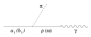
Figure 1: Diagram for the $a_{1}$ and $b_{1}$ decay into $\pi\gamma$ through vector meson dominance.

The case of the $a_{1}$ decay proceeds with the exchange of a $\rho$ meson while the decay of the $b_{1}$ requires the exchange of the $\omega$ meson. In addition to the Lagrangians which we have, we need the vector meson-photon coupling which is given in [14] in the tensor formalism by

$${\cal L}_{V\gamma}=-e\frac{F_{V}}{2}\lambda_{V\gamma}V_{\mu\nu}^{0}(\partial^{\mu}A^{\nu}-\partial^{\nu}A^{\mu})$$ (27)

with $\lambda_{V\gamma}=1,\frac{1}{3},-\frac{\sqrt{2}}{3}$ for $V^{0}=\rho^{0},\omega,\phi$ respectively.

Furthermore one also needs the vector meson propagator in the tensor formalism which is also given in [14] as

$$< 0|T\{W_{\mu\nu}W_{\rho\sigma}\}|0>=i{\cal D}_{\mu\nu\rho\sigma}=$$

$$= i\frac{M_{W}^{-2}}{M_{W}^{2}-P^{2}-i\epsilon}\left[g_{\mu\rho}\,g_{\nu\sigma}\,(M_{W}^{2}-P^{2})+g_{\mu\rho}\,P_{\nu}\,P_{\sigma}-g_{\mu\sigma}\,P_{\nu}\,P_{\rho}-(\mu\leftrightarrow\nu)\right]$$

In view of this, the decay width is given by Eq. (21), where $t$ is now given by

$$t=\frac{2\lambda_{AVP}\lambda_{V\gamma}F_{V}e}{M_{A}M_{V}^{2}}\left(p^{\prime}\cdot p\,\epsilon^{\prime}\cdot\epsilon-\epsilon^{\prime}\cdot p\,\epsilon\cdot p^{\prime}\right)$$ (29)

which exhibits explicitly gauge invariance. Should we have used the vector couplings of Eq. (19) for the $AVP$ plus the vector formalism for the vector-photon coupling of [40], we would have obtained only the term $\epsilon^{\prime}\cdot\epsilon$ which does not fulfill gauge invariance and is unacceptable to represent the process, something that was already pointed out in [43]. On the other hand, should we have use Eqs. (1) and (27), replacing $W_{\mu\nu}$ by $\partial_{\mu}W_{\nu}-\partial_{\nu}W_{\mu}$ and using the standard propagator for $\partial_{\mu}W_{\nu}-\partial_{\nu}W_{\mu}$, (the same as Eq. (3) except for the contact terms proportional to $(M_{W}^{2}-P^{2})$), we would have got zero, indicating that one would have to add contact terms in the vector formalism to make it equivalent to the tensor one, in the line of the claims made in other works trying to show the equivalence between the vector and tensor formalisms [15, 17, 16, 12].

Using the couplings obtained before for the $AVP$ vertices plus those of the $V\gamma$ vertex, we find for the radiative decay width of the $a_{1}$ resonance of $380\pm 50\textrm{ KeV}$, $320\pm 40\textrm{ KeV}$ or $470\pm 60\textrm{ KeV}$ for the solutions $(1)$, $(2)$ and $(3)$ of table 6 respectively, in reasonable good agreement with the experimental value $640\pm 246\textrm{ KeV}$. This is not the case of the $b_{1}$ decay for which we get a width $32\pm 4\textrm{ KeV}$, $36\pm 5\textrm{ KeV}$ or $19\pm 4\textrm{ KeV}$ for the solutions $(1)$, $(2)$ and $(3)$, which is too small compared with experiment, $230\pm 60\textrm{ KeV}$. The reason for this drastic reduction from the $a_{1}$ to the $b_{1}$ is the factor $1/3$ of the $\omega\gamma$ coupling with respect to the $\rho\gamma$ coupling. Since for this reason the vector meson dominance term is so much reduced with respect to the case of the $a_{1}$ decay, it is not surprising that other mechanisms can also account for this decay channel. However, the $b_{1}\to\pi\gamma$ decay width is still much smaller than that of the $a_{1}$, around a factor 3. Such possible mechanisms would thus be smaller than the vector meson dominance mechanisms for the case of the $a_{1}$ decay, in which case the decay width provided by the vector meson dominance mechanism should be relatively accurate as it is the case, accounting for more than $2/3$ of the total $a_{1}\to\pi\gamma$ decay width.

It is interesting to establish comparison of the result obtained here for the radiative decay width of the $a_{1}$ resonance with those of [14]. This comparison can be carried out at the analytical level by recalling the structure of the Lagrangian in [14]

$${\cal L}=\frac{F_{V}}{2\sqrt{2}}\langle A_{\mu\nu}f_{-}^{\mu\nu}\rangle$$ (30)

where $f_{-}^{\mu\nu}$ is defined in [14] and provides, in our case, the pseudoscalars and photon fields. From the Lagrangian of Eq. (30) one can derive the amplitude for the $a_{1}^{+}\to\pi^{+}\gamma$ decay obtaining

$$t=-\frac{iF_{A}e}{fM_{A}}\left(p^{\prime}\cdot p\,\epsilon^{\prime}\cdot\epsilon-\epsilon^{\prime}\cdot p\,\epsilon\cdot p^{\prime}\right)$$ (31)

where $f=92.4\textrm{ MeV}$ and $e$ is taken positive. This latter amplitude can be compared to the one in Eq. (29) using that for the $a_{1}^{+}\to\pi^{+}\gamma$ decay $\lambda_{V\gamma}=1$ and $\lambda_{AVP}=-\sqrt{2}iF$ obtaining that

$$\tilde{F}=\frac{1}{2\sqrt{2}}\frac{F_{A}}{F_{V}}\frac{M_{V}^{2}}{f}$$ (32)

It is interesting to recall that the $F_{A}$ parameter is related, through the Weinberg sum rule [44], to the $F_{V}$ and $f$ parameters by $F_{A}=\sqrt{F_{V}^{2}-f^{2}}$, and using values of $F_{V}$ and $f$ from [14], then $F_{A}\simeq 123\textrm{ MeV}$. Using this value in Eq. (32) one obtains ${\tilde{F}}\simeq 1800\textrm{ MeV}$, to be compared with the values obtained in table 6. It is also interesting to recall that $F_{A}$ is related to the $L_{10}$ coefficient of the second order meson chiral Lagrangian [45] through $L_{10}^{V+A}=-\frac{F_{V}^{2}}{4M_{V}^{2}}+\frac{F_{A}^{2}}{4M_{A}^{2}}$. With the value obtained in our fit for $\tilde{F}$, and consequently for $F_{A}$, the same qualitative agreement obtained in [14] with the empirical value of $L_{10}$ holds also here. This allows to relate the parameter $\tilde{F}$ of our effective Lagrangian (Eq. 1) with the $L_{10}$ parameter of the chiral Lagrangians.

Apart from the comparison of the coefficients at the numerical level, it is also illustrative to compare the analytical expression of the coefficient of Eq. (32) with the corresponding one used in [8]. By using the vector meson dominance values of [14], $F_{V}=\sqrt{2}f$, $F_{A}=f$, $M_{A}=\sqrt{2}M_{V}$, we obtain $\tilde{F}=M_{V}^{2}/4f$, and considering the $a_{1}^{+}\to\rho^{+}\pi^{0}+\rho^{0}\pi^{+}$ and the coefficients of $\lambda_{AVP}$ in Table 2, we obtain, for the coefficient of Eq. (23),

$$\frac{|\lambda_{a_{1}^{+}\rho^{+}\pi^{0}}|^{2}+|\lambda_{a_{1}^{+}\rho^{0}\pi^{+}}|^{2}}{2\pi M_{A}^{2}}=\frac{M_{\rho}^{2}}{16\pi f^{2}}$$ (33)

which coincides with Eq. (2.22) of [8].

We can also perform another study including the experimental $a_{1}\to\pi\gamma$ decay width into the fit, in which case we obtain:

	${\tilde{D}}$ (MeV)	${\tilde{F}}$ (MeV)	$\alpha$ (degrees)	$\chi^{2}/dof$
$(1)$	$-1230\pm 80$	$1380\pm 90$	$62\pm 3$	$0.743$
$(2)$	$-1320\pm 90$	$1270\pm 80$	$29\pm 3$	$0.859$
$(3)$	$-960\pm 90$	$1540\pm 100$	$47\pm 4$	$1.129$

Table 7: Results of the fit including the data of table 4 and the $a_{1}\to\pi\gamma$ decay.

With this final set of parameters we can predict the widths of all the $A\to VP$ decay widths not included in the particle data table. The results for the three possible solutions of table 7 are shown in table 8. We make predictions for all possible decays, many of them yet unobserved. The errors quoted are statistical, but large uncertainties should be assumed in cases where the phase space is only allowed due to the tails of the resonance mass distributions through Eq. 24. It is however instructive to see that all widths predicted are well within the values of the total width of the decaying particle, which we have also written in the table for comparison.

Reaction	$\Gamma_{\textrm{tot}}^{\textrm{exp}}\textrm{ (MeV)}$	$\Gamma_{i}^{\textrm{exp}}\textrm{ (MeV)}$	$\Gamma_{i}\textrm{ (MeV)}$ $(1)$	$\Gamma_{i}\textrm{ (MeV)}$ $(2)$	$\Gamma_{i}\textrm{ (MeV)}$ $(3)$
$a_{1}\to\pi\gamma$	$425\pm 175$	$0.64\pm 0.25$	$0.37\pm 0.05$	$0.31\pm 0.04$	$0.46\pm 0.06$
$K_{1}(1270)\to\rho K$	$90\pm 20$	$38\pm 10$	$48\pm 5$	$46\pm 5$	$47\pm 5$
$K_{1}(1270)\to K^{*}\pi$		$14\pm 6$	$10\pm 4$	$8\pm 4$	$6\pm 4$
$K_{1}(1270)\to\omega K$		$10\pm 3$	$12.8\pm 1.3$	$12.4\pm 1.3$	$12.6\pm 1.4$
$K_{1}(1400)\to K^{*}\pi$	$174\pm 13$	$164\pm 16$	$143\pm 14$	$145\pm 14$	$146\pm 17$
$K_{1}(1400)\to\rho K$		$5\pm 5$	$6\pm 4$	$7\pm 4$	$4\pm 4$
$K_{1}(1400)\to\omega K$		$1.7\pm 1.7$	$2.1\pm 1.2$	$2.4\pm 1.3$	$1.3\pm 1.2$
$b_{1}\to\omega\pi$	$142\pm 9$	$110\pm 40$	$114\pm 14$	$130\pm 18$	$69\pm 14$
$f^{\prime}\to K^{*}K$	$55.5\pm 2.9$	$28\pm 14$	$42\pm 5$	$34\pm 4$	$51\pm 6$
$h\to\rho\pi$	$360\pm 40$	$180\pm 180$	$290\pm 40$	$330\pm 50$	$180\pm 30$
$a_{1}\to\rho\pi$		$210\pm 210$	$260\pm 30$	$220\pm 30$	$320\pm 40$
$h^{\prime}\to K^{*}K$	$91\pm 30$	$45\pm 45$	$42\pm 5$	$48\pm 7$	$25\pm 5$
$a_{1}\to K^{*}K$			$31\pm 4$	$26\pm 3$	$39\pm 5$
$b_{1}\to K^{*}K$			$9.1\pm 1.1$	$10.5\pm 1.4$	$5.6\pm 1.1$
$b_{1}\to\rho\eta$			$16\pm 2$	$18\pm 3$	$9.8\pm 1.9$
$b_{1}\to\rho\eta^{\prime}$			$0.81\pm 0.10$	$0.93\pm 0.13$	$0.49\pm 0.10$
$h\to\omega\eta$			$17\pm 2$	$19\pm 3$	$10\pm 2$
$h\to\omega\eta^{\prime}$			$2.5\pm 0.3$	$2.9\pm 0.4$	$1.6\pm 0.3$
$h\to K^{*}K$			$17.7\pm 2$	$20\pm 3$	$11\pm 2$
$h^{\prime}\to\phi\eta$			$2.2\pm 0.3$	$2.6\pm 0.4$	$1.4\pm 0.3$
$h^{\prime}\to\phi\eta^{\prime}$			$0.43\pm 0.05$	$0.49\pm 0.07$	$0.26\pm 0.05$
$f\to K^{*}K$	$24.0\pm 1.2$		$3.8\pm 0.5$	$3.2\pm 0.4$	$4.8\pm 0.6$

Table 8: Partial widths obtained for all the $A\to VP$ decays with the three different possible solutions of the $\tilde{D}$, $\tilde{F}$ and $\alpha$ parameters. The theoretical errors shown are only due to the uncertainties in these parameters.

Recently, a paper dealing with $\tau\to\pi\pi\pi\nu_{\tau}$ has appeared [46] in which five different structures to account for the $AVP$ coupling in the tensor formalism have been derived. Although the structures derived there are formally different to the one we propose, it is easy to see that at tree level the terms $O^{4}$ and $O^{5}$ of Eq. (12) of [46] give an identical structure for the amplitude to that of our Lagrangian and so would do a linear combination of $O^{2}$ and $O^{3}$ . The $O^{1}$, however, breaks explicitly $SU(3)$ symmetry and hence has no room in our $SU(3)$ symmetric approach. In practical terms, the results of the present work indicate that should one use the formalism of [46] at tree level to deal with $A\to VP$ decay, one would obtain very good agreement with the data by taking, for instance, the $O^{4}$ term alone. This, of course, affects only the octet of the $a_{1}$, not the $b_{1}$ which we have also studied here.

4 Summary

We have addressed the decay of an axial-vector into a vector and a pseudoscalar meson looking for a Lagrangian which can reproduce all existing data while making predictions for all yet unobserved allowed channels involving all the particles of the $SU(3)$ nonets. We found that a basic Lagrangian involving commutator and anticommutator of the fields, using the tensor representation for the vector and axial-vector mesons, was rather accurate and, at the same time, simple enough to be used in intermediate steps of more complicated hadronic processes.

We have also shown that the combination of our $AVP$ Lagrangian with Vector Meson Dominance leads to an amplitude for the radiative decay of the $a_{1}$ into $\pi\gamma$, which formally agrees with the one obtained in the chiral formulation of vector meson and axial couplings, relating the $\tilde{F}$ parameter of the $AVP$ coupling to the $F_{V}$ parameter of the $V\gamma$ coupling in VMD and to the coefficients of the meson chiral Lagrangians. The tensor formalism produces small numerical differences in the predictions for the different decays of the axial-vector mesons with respect to the vector formalism without derivatives, yet it leads naturally to a gauge invariant amplitude for the radiative decay of the $a_{1}$ resonance while this vector formalism leads to a non invariant one. From the studied strong decays we found three acceptable solutions for the parameters and the mixing angle of the strange axial-vectors, with two of them with angles around $30$ and $60$ degrees, slightly favored with respect the solution around $45$ degrees. This is the maximum information that can be obtained from all the $A\to VP$ present decay data. The present determination of the mixing angle has the advantage from previous works of using all the $A\to VP$ available decay data, not only $K_{1}$ decays, and of considering the dynamics given by a suitable Lagrangian. Regarding the prediction for unobserved channels, it is interesting to observe that all the predicted decay rates are well within the boundaries of the total decay widths. Since the predictions of the three different solutions for some channels are quite different, the measurement of some of them would be most welcome in order to find out the actual mixing and the value of the coupling parameters.

The simple form derived for the Lagrangian has made easier the implementation of mechanisms involving exchange of axial-vector mesons which contribute in processes of radiative decays of $\phi$ and $J/\Psi$ which had not been discussed till recently. With tests of hadronic models and particularly chiral dynamics been conducted in physical processes occurring at higher energies, an increasing attention will have to be payed to the role of axial-vector mesons. The work in the present paper makes this task easier.

References

• [1] E. S. Ackleh, T. Barnes and E. S. Swanson, Phys. Rev. D 54 (1996) 6811.
• [2] J. C. R. Bloch, Y. L. Kalinovsky, C. D. Roberts and S. M. Schmidt, Phys. Rev. D 60 (1999) 111502.
• [3] J. Wess and B. Zumino, Phys. Rev.  163 (1967) 1727.
• [4] H. Gomm, O. Kaymakcalan and J. Schechter, Phys. Rev. D 30 (1984) 2345.
• [5] B. R. Holstein, Phys. Rev. D 33 (1986) 3316.
• [6] M. Bando, T. Fujiwara and K. Yamawaki, Prog. Theor. Phys.  79 (1988) 1140.
• [7] U. G. Meissner, Phys. Rept.  161 (1988) 213.
• [8] N. Kaiser and U. G. Meissner, Nucl. Phys. A 519 (1990) 671.
• [9] P. Ko and S. Rudaz, Phys. Rev. D 50 (1994) 6877.
• [10] B. A. Li, Phys. Rev. D 52 (1995) 5165 [arXiv:hep-ph/9504304].
• [11] B. A. Li, Phys. Rev. D 52 (1995) 5184.
• [12] M. C. Birse, Z. Phys. A 355 (1996) 231 [arXiv:hep-ph/9603251].
• [13] J. Gasser and H. Leutwyler, Annals Phys.  158 (1984) 142.
• [14] G. Ecker, J. Gasser, A. Pich and E. de Rafael, Nucl. Phys. B 321 (1989) 311.
• [15] G. Ecker, J. Gasser, H. Leutwyler, A. Pich and E. de Rafael, Phys. Lett. B 223, 425 (1989).
• [16] J. Bijnens and E. Pallante, Mod. Phys. Lett. A 11 (1996) 1069 [arXiv:hep-ph/9510338].
• [17] B. Borasoy and U. G. Meissner, Int. J. Mod. Phys. A 11 (1996) 5183 [arXiv:hep-ph/9511320].
• [18] J. A. Oller and E. Oset, Phys. Rev. D 60 (1999) 074023 [arXiv:hep-ph/9809337].
• [19] M. Jamin, J. A. Oller and A. Pich, JHEP 0402 (2004) 047 [arXiv:hep-ph/0401080].
• [20] J. A. Oller, E. Oset and J. E. Palomar, Phys. Rev. D 63 (2001) 114009 [arXiv:hep-ph/0011096].
• [21] A. Pich and J. Portoles, Phys. Rev. D 63 (2001) 093005 [arXiv:hep-ph/0101194].
• [22] J. R. Pelaez, Phys. Rev. Lett.  92 (2004) 102001 [arXiv:hep-ph/0309292].
• [23] J. A. Oller, E. Oset and J. R. Pelaez, Phys. Rev. D 59 (1999) 074001 [Erratum-ibid. D 60 (1999) 099906] [arXiv:hep-ph/9804209].
• [24] J. Wess and B. Zumino, Phys. Lett. B 37 (1971) 95.
• [25] W. A. Bardeen, Phys. Rev.  184 (1969) 1848.
• [26] J. E. Palomar, L. Roca, E. Oset and M. J. Vicente Vacas, Nucl. Phys. A 729 (2003) 743 [arXiv:hep-ph/0306249].
• [27] M. Uehara, Prog. Theor. Phys.  109 (2003) 265 [arXiv:hep-ph/0211029].
• [28] L. Roca, J. E. Palomar, E. Oset and H. C. Chiang; In preparation
• [29] A. Bramon, R. Escribano, J. L. Lucio Martinez and M. Napsuciale, Phys. Lett. B 517 (2001) 345 [arXiv:hep-ph/0105179].
• [30] J. E. Palomar, S. Hirenzaki and E. Oset, Nucl. Phys. A 707 (2002) 161 [arXiv:hep-ph/0111308].
• [31] H. J. Lipkin, Phys. Lett. B 72 (1977) 249.
• [32] R. Barbieri, R. Gatto and Z. Kunszt, Phys. Lett. B 66 (1977) 349.
• [33] R. K. Carnegie, R. J. Cashmore, W. M. Dunwoodie, T. A. Lasinski and D. W. Leith, Phys. Lett. B 68 (1977) 287.
• [34] M. Suzuki, Phys. Rev. D 47 (1993) 1252.
• [35] H. Y. Cheng, Phys. Rev. D 67 (2003) 094007 [arXiv:hep-ph/0301198].
• [36] H. G. Blundell, S. Godfrey and B. Phelps, Phys. Rev. D 53 (1996) 3712.
• [37] L. Burakovsky and T. Goldman, Phys. Rev. D 56 (1997) 1368 [arXiv:hep-ph/9703274].
• [38] T. Barnes, N. Black and P. R. Page, Phys. Rev. D 68 (2003) 054014.
• [39] M. Suzuki, Phys. Rev. D 55 (1997) 2840 [arXiv:hep-ph/9609479].
• [40] A. Bramon, A. Grau and G. Pancheri, Phys. Lett. B 283 (1992) 416.
• [41] J. Schechter, Private communication
• [42] K. Hagiwara et al. [Particle Data Group Collaboration], Phys. Rev. D 66 (2002) 010001.
• [43] L. Xiong, E. V. Shuryak and G. E. Brown, Phys. Rev. D 46 (1992) 3798 [arXiv:hep-ph/9208206].
• [44] S. Weinberg, Phys. Rev. Lett.  18 (1967) 507.
• [45] J. Gasser and H. Leutwyler, Nucl. Phys. B 250 (1985) 465.
• [46] D. Gomez Dumm, A. Pich and J. Portoles, Phys. Rev. D 69 (2004) 073002 [arXiv:hep-ph/0312183].