Helicity Formalism for Spin-2 Particles

Abstract:

We develop the helicity formalism for spin-2 particles and apply it to the case of gravity in flat extra dimensions. We then implement the large extra dimensions scenario of Arkani-Hamed, Dimopoulos and Dvali in the program AMEGIC++, allowing for an easy calculation of arbitrary processes involving the emission or exchange of gravitons. We complete the set of Feynman rules derived by Han, Lykken and Zhang, and perform several consistency checks of our implementation.

1 Introduction

We have learned from string theory that extra spatial dimensions are the price for unifying the Standard Model with gravity. Yet we are practically ignorant about how and why these extra dimensions are hidden from our world. Will they appear at the electroweak scale? Are they bosonic or fermionic? We hope that the answers to these puzzling questions are awaiting us in the next round of collider experiments at the Tevatron, LHC, and, possibly, at the next linear collider.

If spatial extra dimensions exist and are accessible to at least some of the Standard Model fields, they have to be very small, $\leq{\cal O}({\rm TeV}^{-1})$. However, it is conceivable that all Standard Model particles are confined to a brane, and only gravity (which is rather poorly tested at short distances) is allowed to permeate the bulk. This is the classic scenario of large extra dimensions [1, 2], from now on referred to as ADD. In ADD the experimental limits on the size of the extra dimensions are much weaker. For recent compilations of various experimental probes of large extra dimensions, see e.g. [3, 4, 5].

Such scenarios offer an alternative solution to the gauge hierarchy problem and new avenues for unifying the Standard Model interactions with gravity. They also predict a variety of novel signals, which are already testable at high-energy colliders, see [6] and references therein. Generally speaking, there are two classes of signatures: real graviton production [7, 8, 9, 10, 11, 12] and virtual graviton exchange [8, 9, 13]. Gravitons have enormous lifetime and decay off the brane, hence real graviton production results in generic missing energy signatures. Virtual graviton exchange may generate numerous higher dimension operators, contributing to the production of fermion [8, 9, 13, 14], gauge boson [15, 16, 17] or Higgs boson [18, 19] pairs, as well as more complicated final states with more than two particles [20, 21].

The phenomenology of ADD extra dimensions has been studied rather extensively, and numerous experimental bounds from LEP and the Tevatron on the scale of extra dimensions $M_{s}$ have been set, yet none of the existing general purpose Monte Carlo event generators has fully and consistently implemented the ADD model. For example, PYTHIA [22] now allows only for the production of narrow graviton resonances as in Randall–Sundrum-type models [23, 24]. Virtual graviton exchange is not implemented. For Run I analyses [25, 26, 27] of large extra dimensions, the Tevatron collaborations have been using an unofficial version of PYTHIA, where ADD graviton production has been implemented as an external process [28]. The situation with HERWIG [29] is very similar – narrow graviton resonances are included [30, 31], but not much else. ISAJET [32] has recently added the process of real ADD graviton production in association with a jet or a photon [33] and the implementation is analogous to [28]. PANDORA [34] has implemented virtual graviton exchange for $e^{+}e^{-}\to f\bar{f},\gamma\gamma,ZZ,W^{+}W^{-}$ with the contact interaction of [13] as well as $e^{+}e^{-}\to\gamma G$ as in [7]. Finally, programs such as Madgraph [35] or COMPHEP [36], although highly automated, do not contain spin-2 particles and thus cannot be applied for graviton studies in their present form. Given all this, the pressing need for an automated event generator, capable of studying ADD phenomenology in its full generality, becomes quite evident.

The ADD Feynman rules have appeared in [8, 9] , so it may seem that implementing the ADD model in one of the above-mentioned event generators is rather straightforward. However, apart from a few simple cases of two-body final states, the calculations involve a large number of diagrams, whose evaluation through the standard textbook methods of squaring the amplitudes, employing the completeness relations and taking the traces, becomes prohibitively difficult. This problem is considerably alleviated when the helicity method is used, which avoids lengthy matrix multiplications stemming from the notorious chains of Dirac matrices. First ideas pointing into this direction can be found in [37, 38]; later on, different approaches were formulated in [39, 40, 41, 42, 43, 44, 45, 46, 47, 48, 49] and further refined in [50, 51, 52]. Thanks to their easy implementation and automatization (see for instance [53, 54, 55]) helicity methods have become a cornerstone for modern programs dealing with the evaluation of cross sections for multi-particle final states. Examples for such programs are the multi-purpose matrix element generators GRACE [56], HELAC [57], O’MEGA [58], AMEGIC++ [59], ALPGEN [60], and Madgraph [35]; furthermore there is a large number of more specialized codes such as those described in [61, 62, 63].

The main purpose of this paper is to develop the helicity formalism for spin-2 particles and to implement the ADD scenario in AMEGIC++ (A Matrix Element Generator In C++). Previous studies of ADD extra dimensions using helicity amplitudes can be found in [12, 34].

The outline of the paper is as follows. In Section 2 we review the basics of the helicity formalism and discuss some ideas (2.4 and 2.5) that allow a general extension to the case of spin-2 particles (gravitons). In Section 3 we specify to the case of ADD and highlight some features of the specific implementation in AMEGIC++. For the main part we follow the conventions of [9]. We describe both external and virtual graviton processes and list a couple of Feynman rules that had not been published before. Section 4 compares this implementation to some existing results in the literature, while Section 5 contains our conclusions. Several novel studies of ADD phenomenology at current and future colliders will be presented in a separate publication [64].

2 The Helicity Method

The basic idea behind the helicity method is to replace Dirac matrices by suitable spinor products, and to use the fact that expressions like

$$\bar{u}(\lambda_{1},\,p_{1})u(\lambda_{2},\,p_{2})$$

are simple scalar functions of the helicities $\lambda$ and the momenta $p$ of the spinors.

2.1 Spinor basis

The spinor basis used in AMEGIC++ follows closely the definitions of [51, 52], where spinors are defined in such a way that they satisfy the Dirac equations

$$p\!\!\!/u(p)=+m\cdot u(p)\;,\;\;p\!\!\!/v(p)=-m\cdot v(p)\,,$$ (1)

with

$$p\!\!\!/^{2}=p^{2}=m^{2}\,,$$

where $m^{2}$ is not constrained to be positive. For space-like $p$, i.e. $p^{2}<0$, $m$ is purely imaginary, and the resulting phase degeneracy can be lifted by considering eigenstates of $\gamma_{5}s\!\!\!/$. With the polarization vector $s$ satisfying

$$s\cdot p=0\;,\;\;s^{2}=-1\,,$$ (2)

this translates into fixing the degeneracy by the conditions

$$\gamma_{5}s\!\!\!/u(p,\pm)=\pm u(p,\pm)\;,\;\;\gamma_{5}s\!\!\!/v(p,\pm)=\pm v(p,\pm)\,.$$ (3)

Spinors can now be constructed explicitly along the lines of [47]. Defining two orthogonal auxiliary vectors $k_{0,1}$ with

$$k_{0}^{2}=0\;,\;\;k_{1}^{2}=-1\;,\;\;k_{0}\cdot k_{1}=0\;,$$ (4)

massless spinors $w$ can be defined through

$$w(k_{0},\lambda)\bar{w}(k_{0},\lambda)=\frac{1+\lambda\gamma_{5}}{2}k\!\!\!/_{0}\,,$$ (5)

and the relative phase between spinors with different helicity is given by

$$w(k_{0},\lambda)=\lambda k\!\!\!/_{1}w(k_{0},-\lambda)\,.$$ (6)

Spinors for an arbitrary four-momentum $p$ with $p^{2}=m^{2}$ can be obtained from the massless ones with the help of

$$u(p,\lambda)=\frac{p\!\!\!/+m}{\sqrt{2p\cdot k_{0}}}w(k_{0},-\lambda)\;,\;\;v(p,\lambda)=\frac{p\!\!\!/-m}{\sqrt{2p\cdot k_{0}}}w(k_{0},-\lambda)\,,$$ (7)

both satisfying Eqs. (1) and (3) . In this approach, conjugate spinors are defined to satisfy relations similar to those of Eq. (3),

$$\bar{u}(p,\pm)\gamma_{5}s\!\!\!/=\pm\bar{u}(p,\pm)\;,\;\;\bar{v}(p,\pm)\gamma_{5}s\!\!\!/=\pm\bar{v}(p,\pm)\,,$$ (8)

and their relation to the massless spinors is given by

$$\bar{u}(p,\lambda)=\bar{w}(k_{0},-\lambda)\frac{p\!\!\!/+m}{\sqrt{2p\cdot k_{0}}}\;,\;\;\bar{v}(p,\lambda)=\bar{w}(k_{0},-\lambda)\frac{p\!\!\!/-m}{\sqrt{2p\cdot k_{0}}}\,.$$ (9)

This guarantees the orthogonality of the spinors and after normalizing

$$\frac{\bar{u}(p,\lambda)u(p,\lambda)}{2m}=1\;,\;\;\frac{\bar{v}(p,\lambda)v(p,\lambda)}{2m}=1\;,$$ (10)

the following completeness relation holds true:

$$1=\sum_{\lambda}\frac{u(p,\lambda)\bar{u}(p,\lambda)-v(p,\lambda)\bar{v}(p,\lambda)}{2m}\,.$$ (11)

2.2 Fermion lines

In particular, the numerators of fermion propagators experience the following manipulation

$$(p\!\!\!/+m)=\frac{1}{2}\sum\limits_{\lambda}\left[\left(1+\frac{m}{\sqrt{p^{2}}}\right)u(p,\lambda)\bar{u}(p,\lambda)+\left(1-\frac{m}{\sqrt{p^{2}}}\right)v(p,\lambda)\,\bar{v}(p,\lambda)\right]\,,$$ (12)

which is valid also for space-like $p$, i.e. for $p^{2}<0$. For a more detailed derivation, see [52]. This replacement allows us to “cut” diagrams into pieces with no internal fermion lines.

2.3 External gauge bosons

For spin-1 bosons there are two different strategies to deal with the polarization vectors:

1. either replace them by spinor products, or

2. define explicit polarization 4-vectors.

Both options are available in AMEGIC++.

2.3.1 Replacing polarization vectors by spinor products

In this section, the replacement of polarization vectors of external massless or massive spin-1 bosons by spinor products is briefly summarized.

• Massless spin-1 bosons on their mass-shell have two physical degrees of freedom; hence their polarization vectors satisfy

  $$\begin{array}[]{llllll}\epsilon_{\mu}(p,\lambda)\,p^{\mu}&=&0\,,&\epsilon_{\mu}(p,\lambda)\,\epsilon^{\mu}(p,\lambda)&=&0\,,\\ \epsilon_{\mu}(p,-\lambda)&=&\epsilon_{\mu}^{*}(p,\lambda)\,,&\epsilon_{\mu}(p,\lambda)\,\epsilon^{\mu}(p,-\lambda)&=&-1\,,\end{array}$$ (15)

  where $p$ and $\lambda$ are the four-momentum and the polarization label of the boson, respectively. In the axial gauge the polarization sum reads

  $$\sum_{\lambda=\pm}\epsilon_{\mu}(p,\lambda)\epsilon_{\nu}^{*}(p,\lambda)=-\eta_{\mu\nu}+\frac{p_{\mu}q_{\nu}+p_{\nu}q_{\mu}}{p\cdot q}\,,$$ (16)

  where the auxiliary vector $q\nparallel p$ and $\eta_{\mu\nu}$ denotes the flat metric tensor. Then, it can be shown that the replacement of the polarization vectors through

  $$\epsilon_{\mu}(p,\,\lambda)=\frac{1}{\sqrt{4p\cdot q}}\,\bar{u}(q,\lambda)\gamma_{\mu}u(p,\lambda)$$ (17)

  satisfies all relations of Eqs. (15) and (16) and is thus a good choice.

• For massive vector bosons one chooses a similar strategy to construct a spinor expression replacing the polarization vectors. However, massive spin-1 bosons on their mass-shell have an additional degree of freedom, the two transverse polarizations are supplemented with a longitudinal one with $\lambda=0$. This state obeys

  $$\epsilon_{\mu}(p,0)\,p^{\mu}=0\;,\;\; \epsilon_{\mu}(p,0)\,\epsilon^{\mu}(p,\lambda)=0\;,\;\;\epsilon_{\mu}(p,0)\,\epsilon^{\mu}(p,0)=-1\,,$$ (18)

  and the corresponding spin sum becomes

  $$\sum_{\lambda=\pm,0}\epsilon_{\mu}(p,\lambda)\epsilon_{\nu}^{*}(p,\lambda)=-\eta_{\mu\nu}+\frac{p_{\mu}p_{\nu}}{m^{2}}\,,$$ (19)

  where $p$ and $m$ are the four-momentum and the mass of the boson. In general, there is no simple replacement for the polarization vectors as for the massless case. However, for unpolarized cross sections, the only relevant requirement is that Eq. (19) be reproduced. This can be simply achieved by introducing vectors and kinematics related to a pseudo-decay of the boson into two massless spinors with momenta $r_{1,2}$ satisfying

  $$r_{1}^{2}=r_{2}^{2}=0\;,\;\;r_{1}^{\mu}+r_{2}^{\mu}=p^{\mu}\,.$$ (20)

  Obviously the quantity

  $$a_{\mu}=\bar{u}(r_{2},-)\gamma_{\mu}u(r_{1},-)$$ (21)

  projects out any scalar off-shell polarization. This quantity can be used to replace the polarization vector, because the integral over the solid angle $\Omega$ of $r_{1}$ available for the decay leads, up to a constant normalization factor, to the spin sum of Eq. (19),

  $$\frac{3}{8\pi m^{2}}\int d\Omega\,a_{\mu}a_{\nu}^{*}=-\eta_{\mu\nu}+\frac{p_{\mu}p_{\nu}}{m^{2}}\,.$$ (22)

  Therefore, replacing

  $$\epsilon_{\mu}\to a_{\mu}\;,\;\;\sum_{\lambda=\pm,0}\epsilon_{\mu}\epsilon_{\nu}^{*}\to\frac{3}{8\pi m^{2}}\int d\Omega\,a_{\mu}a_{\nu}^{*}$$ (23)

  leads to the desired result. A first discussion of these ideas can be found in [45].

2.3.2 Polarization basis

It often turns out to be more convenient to keep the polarizations explicitly. A possible choice for an on-shell vector boson with momentum

$$p_{\mu}=\left(p_{0},\left|\vec{p}\right|\sin\theta\cos\varphi,\left|\vec{p}\right|\sin\theta\sin\varphi,\left|\vec{p}\right|\cos\theta\right)$$

is

$$\begin{array}[]{llllll}\epsilon_{\mu}^{\pm}(p)&=&\frac{1}{\sqrt{2}}\left(0,\cos\theta\cos\varphi\mp i\sin\varphi,\cos\theta\sin\varphi\pm i\cos\varphi,-\sin\theta\right)\\ \epsilon_{\mu}^{0}(p)&=&\frac{1}{\sqrt{p^{2}}}\left(\left|\vec{p}\right|,p_{0}\frac{\vec{p}}{\left|\vec{p}\right|}\right).\end{array}$$ (26)

For the special choice of $q=\left(p_{0},-\vec{p}\right)$ this satisfies Eq. (15) and Eq. (16) for a massless boson; for massive bosons, also Eq. (18) and Eq. (19) are fulfilled.

Note that from now on we will label the polarization mode with an upper index. To avoid confusion, Lorentz indices are always denoted by $\mu,\nu,\rho$ or $\sigma$, while $\lambda$ and $\kappa$ are used to indicate a vector polarization mode.

2.4 Gauge boson propagators

Similar to the external vector boson treatment, there are two strategies to deal with gauge boson propagators:

• Structures in Feynman amplitudes with internal boson lines are calculated as one function (composite building block), depending just on the spinors at its edges. (External vector bosons are replaced as in 2.3.1.)

• The numerator of vector boson propagators can be replaced by products of polarization vectors similar to the completeness relations in Eq. (16) and Eq. (19). This allows us to “cut” internal boson lines.

The replacement of the numerator for a massive spin-1 boson in unitary gauge reads

$$\sum_{\lambda=t_{1},t_{2},l,s}\epsilon_{\mu}^{\lambda}(p)\epsilon_{\nu}^{\lambda}(p)=-\eta_{\mu\nu}+\frac{p_{\mu}p_{\nu}}{m^{2}},$$ (27)

where $p_{\mu}=\left(p_{0},\left|\vec{p}\right|\sin\theta\cos\varphi,\left|\vec{p}\right|\sin\theta\sin\varphi,\left|\vec{p}\right|\cos\theta\right)$ can now be off-shell. The corresponding polarization vectors are

$$\epsilon_{\mu}^{t_{1}}(p) = \left(0,\cos\theta\cos\varphi,\cos\theta\sin\varphi,-\sin\theta\right)\,,$$

$$\epsilon_{\mu}^{t_{2}}(p) = \left(0,-\sin\varphi,\cos\varphi,0\right)\,,$$

$$\epsilon_{\mu}^{l}(p) = \frac{1}{\sqrt{p^{2}}}\left(\left|\vec{p}\right|,p_{0}\frac{\vec{p}}{\left|\vec{p}\right|}\right)\,,$$

$$\epsilon_{\mu}^{s}(p) = \sqrt{\frac{p^{2}-m^{2}}{p^{2}m^{2}}}p_{\mu}\,,$$ (28)

with the physical boson mass $m$. To simplify the implementation we choose a basis with linear polarization vectors $\epsilon_{\mu}^{t_{1}}$ and $\epsilon_{\mu}^{t_{2}}$ for the transverse modes. Together with the longitudinal mode $\epsilon_{\mu}^{l}$ these vectors yield Eq. (19) for particles on their mass-shell. They are normalized and orthogonal. The scalar polarization $\epsilon_{\mu}^{s}$ reflects the “off-shellness” of the propagating particle. The orthogonality to all other polarization vectors is obvious, since it is proportional to $p_{\mu}$. Note that in Eq. (27) there is no complex conjugation in the polarization product. This avoids an extra sign discussion for space-like $p$, where $\epsilon_{\mu}^{l}$ and $\epsilon_{\mu}^{s}$ may become imaginary. The above replacement is also valid for vector bosons with a width, if $m^{2}$ is substituted by $m^{2}+im\Gamma$.

A simple inspection of Eq. (27) shows that a similar relation for massless vector bosons can be obtained by taking the limit $m\rightarrow\infty$. Then, only $\epsilon_{\mu}^{s}$ is affected and turns out to be

$$\epsilon_{\mu}^{s_{0}}(p) = \sqrt{-\frac{1}{p^{2}}}\ p_{\mu}.$$ (29)

By contracting the corresponding Lorentz index in each of the neighbouring vertices with a polarization vector and summing over the degrees of freedom, the Lorentz structure of the propagator is absorbed.

2.5 Spin-2 bosons

In this section we will show how the above ideas can be extended to deal with spin-2 particles. We follow the conventions and Feynman rules derived in [9]. With some minimal changes, this can be applied to other models involving quantum gravity as well [23, 24].

The propagator for a KK-graviton with mass $m$ is

$$i\triangle_{\{\mu\nu\},\{\rho\sigma\}}(p)=\frac{iB_{\mu\nu,\rho\sigma}(p)}{p^{2}-m^{2}+i\varepsilon},$$ (30)

where

$$B_{\mu\nu,\rho\sigma}(p) = \frac{1}{2}\left(\eta_{\mu\rho}-\frac{p_{\mu}p_{\rho}}{m^{2}}\right)\left(\eta_{\nu\sigma}-\frac{p_{\nu}p_{\sigma}}{m^{2}}\right)+\frac{1}{2}\left(\eta_{\mu\sigma}-\frac{p_{\mu}p_{\sigma}}{m^{2}}\right)\left(\eta_{\nu\rho}-\frac{p_{\nu}p_{\rho}}{m^{2}}\right)$$ (31)

$$-\frac{1}{3}\left(\eta_{\mu\nu}-\frac{p_{\mu}p_{\nu}}{m^{2}}\right)\left(\eta_{\rho\sigma}-\frac{p_{\rho}p_{\sigma}}{m^{2}}\right).$$

Employing Eq. (27) for each term in parentheses, we obtain

$$B_{\mu\nu,\rho\sigma} = \sum_{\lambda,\kappa=t_{1},t_{2},l,s}\left(\frac{1}{2}\epsilon_{\mu}^{\lambda}\epsilon_{\rho}^{\lambda}\epsilon_{\nu}^{\kappa}\epsilon_{\sigma}^{\kappa}+\frac{1}{2}\epsilon_{\mu}^{\lambda}\epsilon_{\sigma}^{\lambda}\epsilon_{\nu}^{\kappa}\epsilon_{\rho}^{\kappa}-\frac{1}{3}\epsilon_{\mu}^{\lambda}\epsilon_{\nu}^{\lambda}\epsilon_{\rho}^{\kappa}\epsilon_{\sigma}^{\kappa}\right).$$ (32)

Since the graviton couples to the energy–momentum tensor, all resulting vertices are symmetric in $\mu\leftrightarrow\nu$. Using this symmetry the above equation can be simplified to

$$B_{\mu\nu,\rho\sigma}=\sum_{\lambda,\kappa=t_{1},t_{2},l,s}\left(\epsilon_{\mu}^{\lambda}\epsilon_{\rho}^{\lambda}\epsilon_{\nu}^{\kappa}\epsilon_{\sigma}^{\kappa}-\frac{1}{3}\epsilon_{\mu}^{\lambda}\epsilon_{\nu}^{\lambda}\epsilon_{\rho}^{\kappa}\epsilon_{\sigma}^{\kappa}\right).$$ (33)

The polarization vectors $\epsilon^{\lambda}$ have been defined in the previous section. To absorb the Lorentz structure of a spin-2 propagator into the vertices, their Lorentz indices now have to be contracted by two polarization vectors and the double sum in Eq. (33) has to be performed.

External spin-2 particles can be described by polarization tensors. A possible choice is given in [9] :

$$\epsilon_{\mu\nu}^{k}=\left\{\epsilon_{\mu}^{+}\epsilon_{\nu}^{+},\frac{1}{\sqrt{2}}\left(\epsilon_{\mu}^{+}\epsilon_{\nu}^{0}+\epsilon_{\mu}^{0}\epsilon_{\nu}^{+}\right),\frac{1}{\sqrt{6}}\left(\epsilon_{\mu}^{+}\epsilon_{\nu}^{-}+\epsilon_{\mu}^{-}\epsilon_{\nu}^{+}-2\epsilon_{\mu}^{0}\epsilon_{\nu}^{0}\right),\frac{1}{\sqrt{2}}\left(\epsilon_{\mu}^{-}\epsilon_{\nu}^{0}+\epsilon_{\mu}^{0}\epsilon_{\nu}^{-}\right),\epsilon_{\mu}^{-}\epsilon_{\nu}^{-}\right\}.$$ (34)

Again applying the $\mu\leftrightarrow\nu$ symmetry in the vertices, this simplifies to

$$\epsilon_{\mu\nu}^{k}=\left\{\epsilon_{\mu}^{+}\epsilon_{\nu}^{+},\sqrt{2}\,\epsilon_{\mu}^{+}\epsilon_{\nu}^{0}\,,\sqrt{\frac{2}{3}}\left(\epsilon_{\mu}^{+}\epsilon_{\nu}^{-}-\epsilon_{\mu}^{0}\epsilon_{\nu}^{0}\right),\sqrt{2}\,\epsilon_{\mu}^{-}\epsilon_{\nu}^{0}\,,\epsilon_{\mu}^{-}\epsilon_{\nu}^{-}\right\}.$$ (35)

Here, $\epsilon_{\mu}^{\pm,0}$ are the usual polarization vectors for massive vector bosons, which were defined in Section 2.3.2. All polarization tensors are normalized and orthogonal, and they fulfill the completeness relation

$$\sum_{k=1...5}\epsilon_{\mu\nu}^{k}\epsilon_{\rho\sigma}^{k}=B_{\mu\nu,\rho\sigma}\;.$$ (36)

2.6 Construction of building blocks

Utilizing the manipulations discussed above, all possible Feynman amplitudes can be built up from a small set of basic building blocks. Denoting all spinors by $u$, defining chirality projectors $P_{L,R}$ through

$$P_{L,R}=\frac{1\mp\gamma_{5}}{2}$$ (37)

and defining

$$\eta_{i}=\sqrt{2p_{i}\cdot k_{0}}\;,\;\;\mu_{i}=\pm\frac{m_{i}}{\eta_{i}},$$ (38)

where $+/-$ refers to particle/antiparticle, the basic building blocks are as follows:

1. Basic functions are direct products of massless spinors of the form

   $$S(\lambda;p_{1},p_{2})\equiv\bar{u}(p_{1},\lambda)u(p_{2},-\lambda)\,.$$ (39)

   Expressed through the auxiliary vectors $k_{0,1}$, they read

   $$S(\pm;p_{1},p_{2}) = 2\frac{\pm(p_{1}\cdot k_{0})(p_{2}\cdot k_{1})\mp(p_{1}\cdot k_{1})(p_{2}\cdot k_{0})-i\epsilon_{\mu\nu\rho\sigma}p_{1}^{\mu}p_{2}^{\nu}k_{0}^{\rho}k_{1}^{\sigma}}{\eta_{1}\eta_{2}}\,,$$

   $$S(\pm;p_{1},p_{2}) = -S(\pm;p_{2},p_{1})\,.$$ (40)

2. The simplest structure is the direct product of two (possibly massive) spinors of the form

   $$Y(p_{1},\lambda_{1};p_{2},\lambda_{2};{c_{R},c_{L}})\equiv\bar{u}(p_{1},\lambda_{1})\left[c_{R}P_{R}+c_{L}P_{L}\right]u(p_{2},\lambda_{2})\,,$$ (41)

   which emerges for instance through couplings of scalar bosons to a fermion current. The results for this function are summarized in Table 1.

   $\lambda_{1}\lambda_{2}$	$Y(p_{1},\lambda_{1};p_{2},\lambda_{2};c_{L},c_{R})$	$\lambda_{1}\lambda_{2}$	$Y(p_{1},\lambda_{1};p_{2},\lambda_{2};c_{L},c_{R})$
   $++$	$c_{R}\mu_{1}\eta_{2}+c_{L}\mu_{2}\eta_{1}$	$+-$	$c_{L}S(+;p_{1},p_{2})$

   Table 1: $Y$-functions for different helicity combinations. Missing combinations can be obtained through the replacements $+\leftrightarrow-$ and $L\leftrightarrow R$.

3. The next basic structure is the product of two spinors with a Dirac matrix in between. This emerges for instance when external gauge bosons couple to fermion lines with the polarization vector of the gauge bosons expressed explicitly or from terms $\sim p^{\mu}p^{\nu}$ of massive gauge boson propagators. This building block is called $X$-function and reads

   $$X(p_{1},\lambda_{1};p_{2};p_{3},\lambda_{3};c_{L},c_{R})=\bar{u}(p_{1},\lambda_{1})p\!\!\!/_{2}[c_{L}P_{L}+c_{R}P_{R}]u(p_{3},\lambda_{3})\,.$$ (42)

   Only the restriction $k_{0}p_{2}\neq 0$ has to be applied by a suitable choice for $k_{0}$. The results for this function are summarized in Table 2.

   $\lambda_{1}\lambda_{3}$	$X(p_{1},\lambda_{1};p_{2};p_{3},\lambda_{3};c_{L},c_{R})$
   $++$	$\mu_{1}\mu_{3}\eta_{2}^{2}c_{L}+\mu_{2}^{2}\eta_{1}\eta_{3}c_{R}+c_{R}S(+;p_{1},p_{2})S(-;p_{2},p_{3})$
   $+-$	$c_{L}\mu_{1}\eta_{2}S(+;p_{2},p_{3})+c_{R}\mu_{3}\eta_{2}S(+;p_{1},p_{2})$

   Table 2: $X$-functions for different helicity combinations. Missing combinations can be obtained through the replacements $+\leftrightarrow-$ and $L\leftrightarrow R$.

4. The last structure to be discussed is

   $$Z(p_{1},\lambda_{1};p_{2},\lambda_{2};p_{3},\lambda_{3};p_{4},\lambda_{4};c_{L}^{12},c_{R}^{12};c_{L}^{34},c_{R}^{34})=$$ (43)

   $$\bar{u}(p_{1},\lambda_{1})\gamma^{\mu}[c_{L}^{12}P_{L}+c_{R}^{12}P_{R}]u(p_{2},\lambda_{2})\bar{u}(p_{3},\lambda_{3})\gamma_{\mu}[c_{L}^{34}P_{L}+c_{R}^{34}P_{R}]u(p_{4},\lambda_{4})\,,$$

   which stems, for example, from terms $\sim\eta^{\mu\nu}$ in gauge boson propagators between fermion lines. Results for this function can be found in Table 3.

   $\lambda_{1}\lambda_{2}\lambda_{3}\lambda_{4}$	$Z(p_{1},\lambda_{1};p_{2},\lambda_{2};p_{3},\lambda_{3};p_{4},\lambda_{4};c_{L}^{12},c_{R}^{12};c_{L}^{34},c_{R}^{34})$
   $++++$	$2\left[S(+;p_{3},p_{1})S(-;p_{2},p_{4})c_{R}^{12}c_{R}^{34}+\mu_{1}\mu_{2}\eta_{3}\eta_{4}c_{L}^{12}c_{R}^{34}+\mu_{3}\mu_{4}\eta_{1}\eta_{2}c_{R}^{12}c_{L}^{34}\right]$
   $+++-$	$2\eta_{2}c_{R}^{12}\left[S(+;p_{1},p_{4})\mu_{3}c_{L}^{34}+S(+;p_{1},p_{3})\mu_{4}c_{R}^{34}\right]$
   $++-+$	$2\eta_{1}c_{R}^{12}\left[S(-;p_{3},p_{2})\mu_{4}c_{L}^{34}+S(-;p_{4},p_{2})\mu_{3}c_{R}^{34}\right]$
   $++--$	$2\left[S(+;p_{4},p_{1})S(-;p_{2},p_{3})c_{R}^{12}c_{L}^{34}+\mu_{1}\mu_{2}\eta_{3}\eta_{4}c_{L}^{12}c_{L}^{34}+\mu_{3}\mu_{4}\eta_{1}\eta_{2}c_{R}^{12}c_{R}^{34}\right]$
   $+-++$	$2\eta_{4}c_{R}^{34}\left[S(+;p_{1},p_{3})\mu_{2}c_{R}^{12}+S(+;p_{2},p_{3})\mu_{1}c_{L}^{12}\right]$
   $+-+-$	$0$
   $+--+$	$-2\left[\mu_{1}\mu_{4}\eta_{2}\eta_{3}c_{L}^{12}c_{L}^{34}+\mu_{2}\mu_{3}\eta_{1}\eta_{4}c_{R}^{12}c_{R}^{34}-\mu_{1}\mu_{3}\eta_{2}\eta_{4}c_{L}^{12}c_{R}^{34}-\mu_{2}\mu_{4}\eta_{1}\eta_{3}c_{R}^{12}c_{L}^{34}\right]$
   $+---$	$2\eta_{3}c_{L}^{34}\left[S(+;p_{4},p_{2})\mu_{1}c_{L}^{12}+S(+;p_{1},p_{4})\mu_{2}c_{R}^{12}\right]$

   Table 3: $Z$-functions for different helicity combinations. Missing combinations can be obtained through the replacements $+\leftrightarrow-$ and $L\leftrightarrow R$.

3 Implementation of the ADD Model

In our implementation of the ADD model we have applied the formalism developed in [9]. We assume $n$ flat extra dimensions of common size $R$, compactified on an $n$-dimensional torus. While the size $R$ is unambiguous, it has become customary in the literature to quote bounds on the size of the extra dimensions in terms of an energy scale $M$, for which there are several popular conventions [8, 9, 13]. We choose to work with the scale $M_{S}$ as defined in the revised version of [9]:

$$R^{n}=\frac{(4\pi)^{n/2}\Gamma(n/2)}{2M_{S}^{n+2}G_{N}},$$ (44)

where $G_{N}=1/(8\pi\bar{M}_{P}^{2})$ is the 4-dimensional Newton’s constant, with $\bar{M}_{P}=2.4\times 10^{18}$ GeV the reduced Planck scale. The other commonly used scale, $M_{D}$, introduced in [8] is related to $M_{S}$ as

$$M_{S}=2\sqrt{\pi}\ \left[\Gamma(n/2)\right]^{1/(n+2)}M_{D}.$$ (45)

Virtual graviton exchange processes are sometimes parametrized in terms of higher dimension operators whose coefficients are suppressed by a scale $\Lambda_{T}$ [8] or $M_{S}^{JH}$ [13]. The relation to $M_{S}$ can be obtained, comparing (58) with (59) and (60).

3.1 Summation of the KK states

While the coupling of matter particles to a single graviton is suppressed by the inverse of the 4-dimensional Planck mass $\bar{M}_{P}$, the amplitude of any given process involving gravitons is enhanced by the multiplicity of graviton states. After summing over the tower of the graviton mass states, the effective suppression is only of order $M_{S}$.

3.1.1 Virtual KK particles

The amplitude for any process involving a virtual graviton exchange contains the sum

$$D(s) = \sum_{\vec{n}}\frac{i}{s-m^{2}_{\vec{n}}+i\varepsilon}\ ,$$ (46)

which is most easily calculated by replacing the sum over states of discrete mass

$$m^{2}_{\vec{n}}=\frac{4\pi^{2}\vec{n}^{2}}{R^{2}}$$ (47)

by an integral over a continuous mass distribution [9]. The result for time-like propagators reads

$$D(s) = \frac{s^{n/2-1}}{2M_{s}^{n+2}G_{N}}\left[\pi+2iI(M_{s}/\sqrt{s})\right]\,,$$ (48)

and for space-like propagators it is given by

$$D_{E}(t) = \frac{|t|^{n/2-1}}{2M_{s}^{n+2}G_{N}}(-2i)I_{E}(M_{s}/\sqrt{|t|}),$$ (49)

with

$$I(x) = \left\{\begin{array}[]{ll}\displaystyle-\sum_{k=1}^{n/2-1}\frac{1}{2k}x^{2k}-\frac{1}{2}\log\left(x^{2}-1\right)&\quad n=\rm{even}\\[14.22636pt] \displaystyle-\sum_{k=1}^{(n-1)/2}\frac{1}{2k-1}x^{2k-1}+\frac{1}{2}\log\left(\frac{x+1}{x-1}\right)&\quad n=\rm{odd}\,,\end{array}\right.$$ (52)

$$I_{E}(x) = \left\{\begin{array}[]{ll}\displaystyle(-1)^{n/2+1}\left[\sum_{k=1}^{n/2-1}\frac{(-1)^{k}}{2k}x^{2k}+\frac{1}{2}\log\left(x^{2}+1\right)\right]&\quad n=\rm{even}\\[14.22636pt] \displaystyle(-1)^{(n-1)/2}\left[\sum_{k=1}^{(n-1)/2}\frac{(-1)^{k}}{2k-1}x^{2k-1}+\tan^{-1}(x)\right]&\quad n=\rm{odd}\,.\end{array}\right.$$ (55)

In Eqs. (48) and (49) above, we have used Eq. (44). In both cases, the leading order terms for $M_{s}^{2}\gg s$ are:

$$D_{E}(|t|\rightarrow s)\approx D(s) \approx \left\{\begin{array}[]{ll}\displaystyle\frac{-i}{2M_{s}^{4}G_{N}}\log\left(\frac{M_{s}^{2}}{s}\right)&\quad n=2\\[14.22636pt] \displaystyle\frac{-i}{2M_{s}^{4}G_{N}}\frac{2}{n-2}&\quad n>2\,.\end{array}\right.$$ (58)

By default, we have implemented in the program the complete expressions (48–55). However, for the sake of comparison with previous work on the subject, we have also implemented the leading order approximation (58), as well as the two other scale conventions mentioned earlier. In the GRW convention [8], the sum (46) amounts to

$$D=\frac{-i}{2\Lambda_{T}^{4}G_{N}},$$ (59)

while in the Hewett convention [13], it reads

$$D=\frac{-i\lambda}{\pi(M^{JH}_{s})^{4}G_{N}},$$ (60)

where the unspecified sign $\lambda$ of the amplitude reflects the arbitrariness in the regularization procedure employed in obtaining (48-55).

3.1.2 External KK particles

For real graviton production processes, we must sum over all possible final state gravitons. A single mass state is labeled by the $n$-dimensional vector $\vec{n}=(n_{1},n_{2},...,n_{n})$, where the $n_{i}$ are integer values. The corresponding mass $m_{\vec{n}}$ is given by Eq. (47). The total number of accessible graviton mass states in the KK tower is

$$\frac{1}{n}\frac{\hat{m}^{n}}{M_{s}^{n+2}G_{N}},$$ (61)

with $\hat{m}$ the maximal kinematically allowed graviton mass. The scale $M_{S}$ is defined by Eq. (44). Since this number is enormous, it is impractical to introduce a separate particle label in the program for each graviton of definite mass. Instead, it is easier to treat the graviton tower as a single particle of variable mass, and then add an extra summation over the graviton mass [28, 33]. In this respect, real graviton production is unlike any of the conventional processes implemented in the general purpose event generators, where the particle masses are held fixed.

The summation over the graviton mass can be easily carried out by the Monte Carlo phase-space integrator used in [59]. Any given scattering event produces a single graviton whose mass $m_{\vec{n}}$ is picked at random from a uniform distribution of $\vec{n}$. Thus, to get the total cross section, the weight of every phase space point has to be re-weighted by the factor (61).

3.2 Vertex Feynman Rules

We have implemented all three- and some of the four-point vertices from [9] for both the spin-2 gravitons and the spin-0 dilaton. We also included a triple-Higgs–KK vertex, which together with a four-Higgs–KK vertex, was not previously listed in the literature, to the best of our knowledge. The Feynman rules for these two additional vertices are shown in Figs. 1 and 2.

Figure 1: The triple-Higgs–KK vertex.

Figure 2: The four-Higgs–KK vertex.

Appendix A contains a list of all implemented vertex Feynman rules, translated into the functions defined as building blocks in Section 2.6.

Note that we define the coupling constants $\kappa$ and $\omega$ somewhat differently from [9]. This should not become an issue, since $\kappa$ and $\omega$ are auxiliary variables, and the ADD model is defined entirely through $M_{S}$ and $n$. In the revised version of [9], the spin-2 propagator and the normalization of the polarization tensors have been changed by a factor of 2, which has been absorbed into $\kappa$. We have also rescaled $\omega$ by an extra factor of $\sqrt{n-1}$, which typically arises from the multiplicity of the spin-0 KK particles

$$\kappa=\sqrt{32\pi G_{N}},\;\;\;\;\omega=\sqrt{\frac{n-1}{3(n+2)}}.$$ (62)

With these definitions the vertex Feynman rules can be simply read off from either the published or revised version of [9] and we do not repeat them here.

4 Tests

As a test of our implementation we performed a number of checks, comparing AMEGIC++ results with independent analytical calculations in the literature:

• In order to test 2-fermion production processes mediated by virtual graviton exchange, we calculated the angular distributions for $e^{+}e^{-}\rightarrow\mu^{+}\mu^{-}$, $e^{+}e^{-}\rightarrow b\bar{b}$ and $e^{+}e^{-}\rightarrow c\bar{c}$. We found each one in good agreement with the original work of [13].

  

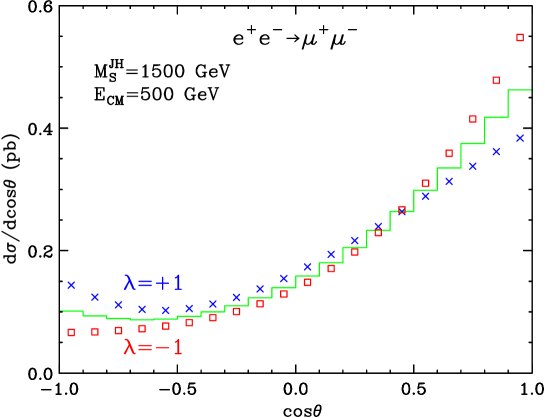
  Figure 3: The AMEGIC++ result for $e^{+}e^{-}\rightarrow\mu^{+}\mu^{-}$, for centre-of-mass energy $E_{CM}=500$ GeV, $M_{S}^{JH}=1500$ GeV, and $\lambda=+1$ (crosses) or $\lambda=-1$ (squares). The solid histogram is the pure Standard Model result.

  Fig. 3 shows the AMEGIC++ result for $e^{+}e^{-}\rightarrow\mu^{+}\mu^{-}$, for a centre-of-mass energy $E_{CM}=500$ GeV. We ran AMEGIC++ in the effective operator mode corresponding to the Hewett convention and chose $M_{S}^{JH}=1500$ GeV. Fig. 3 displays our results for both $\lambda=+1$ (crosses) and $\lambda=-1$ (squares), as well as the pure Standard Model result (solid histogram). We see perfect agreement with Fig. 1 of the archived version of [13]. We also ran AMEGIC++ in its default mode, choosing the appropriate $M_{S}$ according to Eq. (60) and recovered the curve corresponding to $\lambda=+1$, thus confirming the result of [3].

• The unpolarized angular distribution for $e^{+}e^{-}\rightarrow W^{+}W^{-}$ was calculated and found to be consistent with the results of [17].

• All of our results on $\gamma\gamma\rightarrow hh$ were found to be in perfect agreement with those of Ref. [19].

• The total cross sections for $\gamma\gamma\rightarrow\gamma\gamma$ and $e^{+}e^{-}\rightarrow\gamma\gamma$ were calculated and compared with the results of [16]. We find agreement, except for the case $n=2$ in $\gamma\gamma\rightarrow\gamma\gamma$. We believe that the reason for the deviation is that [16] used the approximation $|t|\sim s$ for $t$-channel diagrams, as in Eq. (58), while the more general $t$-channel result is given by Eq. (49).

• We tested real graviton production through $e^{+}e^{-}\rightarrow\gamma G$.

  

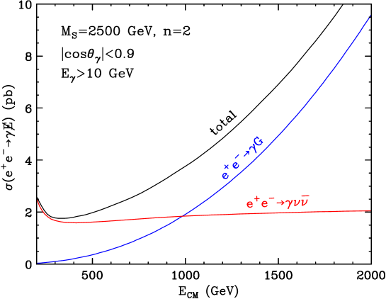
  Figure 4: The total cross-section for $e^{+}e^{-}\rightarrow\gamma G$ as a function of the centre-of-mass energy $E_{CM}$, for $M_{S}=2500$ GeV, $n=2$ and photon energy and angular acceptance cuts of $E_{\gamma}>10$ GeV and $|\cos\theta_{\gamma}|<0.9$, respectively. Compare with Fig. 3 of [10].

  Our results for the total cross section as a function of the centre-of-mass energy $E_{CM}$ are shown in Fig. 4 for $M_{S}=2500$ GeV, $n=2$, and for photon energy and angular acceptance cuts of $E_{\gamma}>10$ GeV and $|\cos\theta_{\gamma}|<0.9$, correspondingly. Fig. 4 agrees very well with the analogous Fig. 3 of [10] .

• Finally, we calculated the decay widths of massive KK particles. For spin-2 KK states we agree with the results of [9]. For spin-0 particles we agree with the results in the original printed version of [9], while in its revised version the widths are too large by a factor of 2.

This implementation of the ADD model will be available in the upcoming version 2.0 of AMEGIC++.

5 Conclusions

The idea that quantum gravity can be relevant already at the TeV scale is extremely attractive – to theorists and experimentalists alike. Since gravity is universal, there exist many potential graviton signatures, but so far only the simplest ones have been explored. The calculations become prohibitively complicated and the need for automation soon becomes evident. Thus the main purpose of this paper was to develop the helicity formalism for spin-2 particles, which could then be used in an automatic event generator, capable of calculating arbitrary processes with gravitons.

Having completed this first task, we proceeded to implement the ADD model of large extra dimensions in AMEGIC++. The large extra dimensions paradigm will soon be tested in collider experiments at the Tevatron, LHC and NLC. We believe that having a simulation tool like AMEGIC++ at our disposal will greatly facilitate the study of new physics related to quantum gravity or extra dimensions. With the general formalism at hand, it is now possible to generalize our implementation to models with warped extra dimensions as well.

Appendix A Appendix:  Vertex Functions

The following shorthands are used:

$$Y_{0} = Y(k_{0},\lambda_{0},k_{0}^{\prime},\lambda_{0}^{\prime},c_{L},c_{R})\,,$$

$$X_{01} = X(k_{0},\lambda_{0},k_{1},k_{0}^{\prime},\lambda_{0}^{\prime},c_{L},c_{R})\,,$$

$$X_{0\kappa} = X(k_{0},\lambda_{0},\epsilon^{\kappa},k_{0}^{\prime},\lambda_{0}^{\prime},c_{L},c_{R})\,,$$

$$Z_{01} = Z(k_{0},\lambda_{0},k_{0}^{\prime},\lambda_{0}^{\prime},k_{1},\lambda_{1},k_{1}^{\prime},\lambda_{1}^{\prime},c_{L}^{0},c_{R}^{0},c_{L}^{1},c_{R}^{1})\,.$$

All spin-2 propagators are “cut” (see 2.4, 2.5), while the spin-1 propagators are attached to a fermion line. For the case when they are attached to something else in a diagram (and for massive vector bosons), they must be “cut” as well. This is done by simple replacements (e.g. to cut the boson line with momentum $p_{0}$):

$$X_{01} \rightarrow \epsilon_{\mu}^{\lambda}k_{1}^{\mu}\,,$$

$$Z_{01} \rightarrow X_{1\lambda}\,,$$

where $\lambda$ labels the polarization modes of the cut line.

Figure 5: The fermion–fermion–KK vertex.

$$FFT = X_{0\lambda}\left(k_{0}\!\cdot\!\epsilon^{\kappa}-k_{0}^{\prime}\!\cdot\!\epsilon^{\kappa}\right)+X_{0\kappa}\left(k_{0}\!\cdot\!\epsilon^{\lambda}-k_{0}^{\prime}\!\cdot\!\epsilon^{\lambda}\right)\,,$$ (A.1)

$$-2\,\epsilon^{\lambda}\!\cdot\!\epsilon^{\kappa}\left(X\left(k_{0},k_{0},k_{0}^{\prime}\right)-X\left(k_{0},k_{0}^{\prime},k_{0}^{\prime}\right)-2m_{\Psi}Y_{0}\right)$$

$$FFGS = X\left(k_{0},k_{0},k_{0}^{\prime}\right)-X\left(k_{0},k_{0}^{\prime},k_{0}^{\prime}\right)-\frac{8}{3}m_{\Psi}Y_{0}\,.$$ (A.2)

Figure 6: The two-gauge-boson–KK vertex.

$$VVT = \left(m_{A}^{2}+p_{0}\!\cdot\!p_{1}\right)\left(X_{0\lambda}X_{1\kappa}+X_{1\lambda}X_{0\kappa}-\epsilon^{\lambda}\!\cdot\!\epsilon^{\kappa}\,Z_{01}\right)$$ (A.3)

$$+\left(X_{01}+X_{00}\right)\left(X_{10}+X_{11}\right)\epsilon^{\lambda}\!\cdot\!\epsilon^{\kappa}+Z_{01}\left(p_{0}\!\cdot\!\epsilon^{\kappa}\;p_{1}\!\cdot\!\epsilon^{\lambda}+p_{1}\!\cdot\!\epsilon^{\kappa}\;p_{0}\!\cdot\!\epsilon^{\lambda}\right)$$

$$-\left(X_{01}+X_{00}\right)\left(X_{1\kappa}\,p_{0}\!\cdot\!\epsilon^{\lambda}+X_{1\lambda}\,p_{0}\!\cdot\!\epsilon^{\kappa}\right)$$

$$-\left(X_{10}+X_{11}\right)\left(X_{0\kappa}\,p_{1}\!\cdot\!\epsilon^{\lambda}+X_{0\lambda}\,p_{1}\!\cdot\!\epsilon^{\kappa}\right)\,,$$

$$VVGS = m_{A}^{2}Z_{01}+X_{00}X_{12}+X_{02}X_{11}\,.$$ (A.4)

Figure 7: The scalar–scalar–KK vertex.

$$SST = \left(m_{\Phi}^{2}+p_{0}\!\cdot\!p_{1}\right)\epsilon^{\lambda}\!\cdot\!\epsilon^{\kappa}-p_{0}\!\cdot\!\epsilon^{\lambda}\;p_{1}\!\cdot\!\epsilon^{\kappa}-p_{1}\!\cdot\!\epsilon^{\lambda}\;p_{0}\!\cdot\!\epsilon^{\kappa}\,,$$ (A.5)

$$SSGS = -2m_{\Phi}^{2}+p_{0}\!\cdot\!p_{1}\,.$$ (A.6)

Figure 8: The fermion–fermion–gauge–boson–KK vertex.

$$FFVT = X_{0\kappa}X_{1\lambda}+X_{1\kappa}X_{0\lambda}-2\,\epsilon^{\lambda}\!\cdot\!\epsilon^{\kappa}Z_{01}\,,$$ (A.7)

$$FFVGS = Z_{01}\,.$$ (A.8)

Figure 9: The triple–gauge–boson–KK vertex.

$$VVVT = A_{012}+A_{120}+A_{210}\,,$$ (A.9)

$$A_{012} = \left(X_{0\lambda}X_{1\kappa}+X_{1\lambda}X_{0\kappa}-\epsilon^{\lambda}\!\cdot\!\epsilon^{\kappa}\,Z_{01}\right)\left(X_{20}-X_{21}\right)$$

$$+Z_{01}\left[X_{2\lambda}(p_{0}\!\cdot\!\epsilon^{\kappa}-p_{1}\!\cdot\!\epsilon^{\kappa})+X_{2\kappa}(p_{0}\!\cdot\!\epsilon^{\lambda}-p_{1}\!\cdot\!\epsilon^{\lambda})\right]\,.$$

Figure 10: The triple–scalar–KK vertex.

List of tables

1. 1 $Y$-functions for different helicity combinations. Missing combinations can be obtained through the replacements $+\leftrightarrow-$ and $L\leftrightarrow R$.
2. 2 $X$-functions for different helicity combinations. Missing combinations can be obtained through the replacements $+\leftrightarrow-$ and $L\leftrightarrow R$.
3. 3 $Z$-functions for different helicity combinations. Missing combinations can be obtained through the replacements $+\leftrightarrow-$ and $L\leftrightarrow R$.

List of figures

1. 1 The triple-Higgs–KK vertex.
2. 2 The four-Higgs–KK vertex.
3. 3 The AMEGIC++ result for $e^{+}e^{-}\rightarrow\mu^{+}\mu^{-}$, for centre-of-mass energy $E_{CM}=500$ GeV, $M_{S}^{JH}=1500$ GeV, and $\lambda=+1$ (crosses) or $\lambda=-1$ (squares). The solid histogram is the pure Standard Model result.
4. 4 The total cross-section for $e^{+}e^{-}\rightarrow\gamma G$ as a function of the centre-of-mass energy $E_{CM}$, for $M_{S}=2500$ GeV, $n=2$ and photon energy and angular acceptance cuts of $E_{\gamma}>10$ GeV and $|\cos\theta_{\gamma}|<0.9$, respectively. Compare with Fig. 3 of [10].
5. 5 The fermion–fermion–KK vertex.
6. 6 The two-gauge-boson–KK vertex.
7. 7 The scalar–scalar–KK vertex.
8. 8 The fermion–fermion–gauge–boson–KK vertex.
9. 9 The triple–gauge–boson–KK vertex.
10. 10 The triple–scalar–KK vertex.

References

- [1] N. Arkani-Hamed, S. Dimopoulos and G. R. Dvali, Phys. Lett. B 429, 263 (1998) [arXiv:hep-ph/9803315].
- [2] I. Antoniadis, N. Arkani-Hamed, S. Dimopoulos and G. R. Dvali, Phys. Lett. B 436, 257 (1998) [arXiv:hep-ph/9804398].
- [3] G. Landsberg, “Extra dimensions and more”, arXiv:hep-ex/0105039.
- [4] J. Hewett and M. Spiropulu, Ann. Rev. Nucl. Part. Sci. 52, 397 (2002) [arXiv:hep-ph/0205106].
- [5] J. Hewett and J. March-Russell, Phys. Rev. D 66, 010001 (2002).
- [6] K. Cheung, “Collider phenomenology for models of extra dimensions”, arXiv:hep-ph/0305003.
- [7] E. A. Mirabelli, M. Perelstein and M. E. Peskin, Phys. Rev. Lett. 82, 2236 (1999) [arXiv:hep-ph/9811337].
- [8] G. F. Giudice, R. Rattazzi, J. D. Wells, Nucl. Phys. B 544, 3 (1999) [arXiv:hep-ph/9811291].
- [9] T. Han, J. D. Lykken, R. Zhang, Phys. Rev. D 59, 105006 (1999) [arXiv:hep-ph/9811350].
- [10] Kingman Cheung, Wai-Yee Keung Phys. Rev. D 60, 112003 (1999) [arXiv:hep-ph/9903294].
- [11] C. Balazs, H. J. He, W. W. Repko, C. P. Yuan and D. A. Dicus, Phys. Rev. Lett. 83, 2112 (1999) [arXiv:hep-ph/9904220].
- [12] T. Han, D. Rainwater and D. Zeppenfeld, Phys. Lett. B 463, 93 (1999) [arXiv:hep-ph/9905423].
- [13] J. L. Hewett, Phys. Rev. Lett. 82, 4765 (1999) [arXiv:hep-ph/9811356].
-
[14]
See, e.g.
P. Mathews, S. Raychaudhuri and K. Sridhar,
Phys. Lett. B 450, 343 (1999)
[arXiv:hep-ph/9811501];
T. G. Rizzo, Phys. Rev. D 59, 115010 (1999) [arXiv:hep-ph/9901209];
P. Mathews, S. Raychaudhuri and K. Sridhar, JHEP 0007, 008 (2000) [arXiv:hep-ph/9904232];
G. Shiu, R. Shrock and S. H. Tye, Phys. Lett. B 458, 274 (1999) [arXiv:hep-ph/9904262];
K. Cheung, Phys. Lett. B 460, 383 (1999) [arXiv:hep-ph/9904510];
D. Bourilkov, JHEP 9908, 006 (1999) [arXiv:hep-ph/9907380];
K. Cheung and G. Landsberg, Phys. Rev. D 62, 076003 (2000) [arXiv:hep-ph/9909218]. -
[15]
See, e.g.
K. Agashe and N. G. Deshpande,
Phys. Lett. B 456, 60 (1999)
[arXiv:hep-ph/9902263];
T. G. Rizzo, Phys. Rev. D 60, 115010 (1999) [arXiv:hep-ph/9904380];
H. Davoudiasl, Phys. Rev. D 60, 084022 (1999) [arXiv:hep-ph/9904425];
D. Atwood, S. Bar-Shalom and A. Soni, Phys. Rev. D 61, 054003 (2000) [arXiv:hep-ph/9906400];
O. J. Eboli, T. Han, M. B. Magro and P. G. Mercadante, Phys. Rev. D 61, 094007 (2000) [arXiv:hep-ph/9908358];
S. Mele and E. Sanchez, Phys. Rev. D 61, 117901 (2000) [arXiv:hep-ph/9909294]. - [16] Kingman Cheung, Phys. Rev. D 61, 015005 (2000) [arXiv:hep-ph/9904266].
- [17] Kang Young Lee, H. S. Song and JeongHyeon Song, Phys. Lett. B 464, 82 (1999) [arXiv:hep-ph/9904355].
- [18] T. G. Rizzo, Phys. Rev. D 60, 075001 (1999) [arXiv:hep-ph/9903475].
- [19] Xiao-Gang He, Phys. Rev. D 60, 115017 (1999) [arXiv:hep-ph/9905295].
- [20] E. Dvergsnes, P. Osland and N. Ozturk, Phys. Rev. D 67, 074003 (2003) [arXiv:hep-ph/0207221].
- [21] N. G. Deshpande and D. K. Ghosh, “Higgs pair production in association with a vector boson at colliders in theories of higher dimensional gravity”, arXiv:hep-ph/0301272.
- [22] T. Sjostrand, L. Lonnblad and S. Mrenna, “PYTHIA 6.2: Physics and manual”, arXiv:hep-ph/0108264.
- [23] L. Randall and R. Sundrum, Phys. Rev. Lett. 83, 3370 (1999) [arXiv:hep-ph/9905221].
- [24] L. Randall and R. Sundrum, Phys. Rev. Lett. 83, 4690 (1999) [arXiv:hep-th/9906064].
- [25] D. Acosta et al. [CDF Collaboration], Phys. Rev. Lett. 89, 281801 (2002) [arXiv:hep-ex/0205057].
- [26] V. M. Abazov et al. [D0 Collaboration], “Search for large extra dimensions in the monojet + missing channel at D0”, arXiv:hep-ex/0302014.
- [27] D. Acosta et al. [CDF Collaboration], ”Search for Kaluza-Klein Graviton Emission in Collisions at TeV using the Missing Energy Signature”, to be submitted to Phys. Rev. Lett. (2003).
- [28] Joseph Lykken and Konstantin Matchev, unpublished.
- [29] G. Corcella et al., “HERWIG 6.5 release note”, arXiv:hep-ph/0210213.
- [30] B. C. Allanach, K. Odagiri, M. A. Parker and B. R. Webber, JHEP 0009, 019 (2000) [arXiv:hep-ph/0006114].
- [31] B. C. Allanach, K. Odagiri, M. J. Palmer, M. A. Parker, A. Sabetfakhri and B. R. Webber, JHEP 0212, 039 (2002) [arXiv:hep-ph/0211205].
- [32] H. Baer, F. E. Paige, S. D. Protopopescu and X. Tata, “ISAJET 7.48: A Monte Carlo event generator for p p, anti-p p, and e+ e- reactions”, arXiv:hep-ph/0001086.
- [33] L. Vacavant and I. Hinchliffe, J. Phys. G 27, 1839 (2001).
- [34] M. E. Peskin, “Pandora: An object-oriented event generator for linear collider physics”, arXiv:hep-ph/9910519.
- [35] F. Maltoni and T. Stelzer, JHEP 0302, 027 (2003) [arXiv:hep-ph/0208156].
- [36] A. Pukhov et al., “CompHEP: A package for evaluation of Feynman diagrams and integration over multi-particle phase space. User’s manual for version 33”, arXiv:hep-ph/9908288.
- [37] M. Jacob and G. C. Wick, Annals Phys. 7, 404 (1959) [Annals Phys. 281, 774 (2000)].
- [38] J. D. Bjorken and M. C. Chen, Phys. Rev. 154 (1966) 1335.
- [39] P. De Causmaecker, R. Gastmans, W. Troost and T. T. Wu, Phys. Lett. B 105, 215 (1981).
- [40] P. De Causmaecker, R. Gastmans, W. Troost and T. T. Wu, Nucl. Phys. B 206, 53 (1982).
- [41] F. A. Berends, R. Kleiss, P. De Causmaecker, R. Gastmans, W. Troost and T. T. Wu, Nucl. Phys. B 206, 61 (1982).
- [42] R. Gastmans and T. T. Wu, “The Ubiquitous Photon: Helicity Method For QED And QCD”, Oxford, UK: Clarendon (1990).
- [43] M. Caffo and E. Remiddi, Helv. Phys. Acta 55, 339 (1982).
- [44] G. Passarino, Phys. Rev. D 28, 2867 (1983).
- [45] G. Passarino, Nucl. Phys. B 237, 249 (1984).
- [46] F. A. Berends, P. H. Daverveldt and R. Kleiss, Nucl. Phys. B 253, 441 (1985).
- [47] R. Kleiss and W. J. Stirling, Nucl. Phys. B 262, 235 (1985).
- [48] R. Kleiss and W. J. Stirling, Phys. Lett. B 179, 159 (1986).
- [49] K. Hagiwara and D. Zeppenfeld, Nucl. Phys. B 274, 1 (1986).
- [50] A. Ballestrero, E. Maina and S. Moretti, Nucl. Phys. B 415, 265 (1994). [arXiv:hep-ph/9212246].
- [51] A. Ballestrero, E. Maina and S. Moretti, “Heavy quark production at colliders in multi-jet events and a new method of computing helicity amplitudes”, arXiv:hep-ph/9405384.
- [52] A. Ballestrero and E. Maina, Phys. Lett. B 350, 225 (1995) [arXiv:hep-ph/9403244].
- [53] H. Tanaka, Comput. Phys. Commun. 58, 153 (1990).
- [54] H. Murayama, I. Watanabe and K. Hagiwara, “HELAS: HELicity Amplitude Subroutines for Feynman diagram evaluations,” KEK-91-11.
- [55] T. Stelzer and W. F. Long, Comput. Phys. Commun. 81, 357 (1994) [arXiv:hep-ph/9401258].
- [56] F. Yuasa et al., Prog. Theor. Phys. Suppl. 138, 18 (2000) [arXiv:hep-ph/0007053].
- [57] A. Kanaki and C. G. Papadopoulos, Comput. Phys. Commun. 132, 306 (2000) [arXiv:hep-ph/0002082].
- [58] T. Ohl, “O’Mega: An optimizing matrix element generator”, arXiv:hep-ph/0011243.
- [59] F. Krauss, R. Kuhn and G. Soff, JHEP 0202, 044 (2002) [arXiv:hep-ph/0109036].
- [60] M. L. Mangano, M. Moretti, F. Piccinini, R. Pittau and A. D. Polosa, “ALPGEN, a generator for hard multiparton processes in hadronic collisions”, arXiv:hep-ph/0206293.
- [61] F. A. Berends, R. Pittau and R. Kleiss, Comput. Phys. Commun. 85, 437 (1995) [arXiv:hep-ph/9409326].
- [62] E. Accomando, A. Ballestrero and E. Maina, Comput. Phys. Commun. 150, 166 (2003) [arXiv:hep-ph/0204052].
- [63] S. Dittmaier and M. Roth, Nucl. Phys. B 642, 307 (2002) [arXiv:hep-ph/0206070].
- [64] T. Gleisberg, F. Krauss, K. Matchev, A. Schälicke, S. Schumann and G. Soff, “Multi-Higgs Signals of Large Extra Dimensions”, in preparation.
- [65] V. V. Andreev, Phys. Rev. D 62, 014029 (2000) [arXiv:hep-ph/0101140]
- [66] F. F. Tikhonin, “An insight into the anatomy of electro-gravitational interactions,” arXiv:hep-ph/0201215.