The decays $\omega(782)\mbox{, }\phi(1020)\to 5\pi$ in the hidden local symmetry approach.

Abstract

The decays $\omega\to 2\pi^{+}2\pi^{-}\pi^{0}$ and $\omega\to\pi^{+}\pi^{-}3\pi^{0}$ are reconsidered in the hidden local symmetry approach (HLS) added with the anomalous terms. The decay amplitudes are analyzed in detail, paying the special attention to the Adler condition of vanishing the whole amplitude at vanishing momentum of any final pion. Combining the Okubo-Zweig-Iizuka (OZI) rule applied to the five pion final state, with the Adler condition, we calculate also the $\phi\to 2\pi^{+}2\pi^{-}\pi^{0}$ and $\phi\to\pi^{+}\pi^{-}3\pi^{0}$ decay amplitudes. The partial widths of the above decays are evaluated, and the excitation curves in $e^{+}e^{-}$ annihilation are obtained, assuming reasonable particular relations among the parameters characterizing the anomalous terms of the HLS Lagrangian. The evaluated branching ratios $B_{\phi\to\pi^{+}\pi^{-}3\pi^{0}}\sim 2\times 10^{-7}$ and $B_{\phi\to 2\pi^{+}2\pi^{-}\pi^{0}}\sim 7\times 10^{-7}$ are such that with the luminosity $L=500\mbox{ pb}^{-1}$ attained at DA$\Phi$NE $\phi$ factory, one may already possess about 1685 events of the decays $\phi\to 5\pi$.

I Introduction

The purpose of the present paper is to calculate the branching ratios of the decays

$$\omega\to\pi^{+}\pi^{-}3\pi^{0},$$ (1)

$$\omega\to 2\pi^{+}2\pi^{-}\pi^{0},$$ (2)

$$\phi\to\pi^{+}\pi^{-}3\pi^{0},$$ (3)

and

$$\phi\to 2\pi^{+}2\pi^{-}\pi^{0},$$ (4)

in the framework of chiral model for pseudoscalar and low lying vector mesons based on hidden local symmetry (HLS) hls1 ; hls2 . This model incorporates vector mesons into chiral theory in a most elegant way. The fact is that the low energy theorems for anomalous processes such as, say, the decay $\pi^{0}\to\gamma\gamma$, are fulfilled automatically in HLS. Since the general form of both nonanomalous and anomalous parts of the Lagrangian is given in Ref. hls1 ; hls2 , we write down here the weak field limit of the above Lagrangian restricted to the subgroup $SU(2)\times U(1)$ with the only isovector $\bm{\pi}$, $\bm{\rho}$, and isoscalar $\omega$ mesons taken into account. Taking into account the coupling of $\phi(1020)$ meson with the mesons composed of nonstrange quarks demands additional assumptions to be discussed below.

The nonanomalous part of the HLS Lagrangian (denoted as $nan$) is obtained from general expression of Ref. hls1 ; hls2 ; schechter and looks as

$$\cal{L}^{\rm nan} = -{1\over 4}\bm{\rho}_{\mu\nu}^{2}-{1\over 4}\omega_{\mu\nu}^{2}+{1\over 2}ag^{2}f_{\pi}^{2}\left(\bm{\rho}^{2}_{\mu}+\omega^{2}_{\mu}\right)+{1\over 2}\left(\partial_{\mu}\bm{\pi}\right)^{2}-{1\over 2}m^{2}_{\pi}\bm{\pi}^{2}+{m^{2}_{\pi}\over 24f^{2}_{\pi}}\bm{\pi}^{4}+$$ (5)

$${1\over 2f^{2}_{\pi}}\left({a\over 4}-{1\over 3}\right)[\bm{\pi}\times\partial_{\mu}\bm{\pi}]^{2}+{1\over 2}ag\left(1-{\bm{\pi}^{2}\over 12f^{2}_{\pi}}\right)\left(\bm{\rho}_{\mu}\cdot[\bm{\pi}\times\partial_{\mu}\bm{\pi}]\right),$$

where the dot ($\cdot$) and cross ($\times$) stand, respectively, for the scalar and vector products in the isotopic space,

$$\bm{\rho}_{\mu\nu} = \partial_{\mu}\bm{\rho}_{\nu}-\partial_{\nu}\bm{\rho}_{\mu}+g[\bm{\rho}_{\mu}\times\bm{\rho}_{\nu}],$$

$$\omega_{\mu\nu} = \partial_{\mu}\omega_{\nu}-\partial_{\nu}\omega_{\mu}$$ (6)

are, respectively, the field strengths of the isovector field $\bm{\rho}_{\mu}$ and the isoscalar field $\omega_{\mu}$, $g$ is the gauge coupling constant, $f_{\pi}=92.4$ MeV is the pion decay constant, while $a$ is HLS parameter. The boldface characters refer hereafter to the vectors in isotopic space. As is clear from Eq. (5),

$$g_{\rho\pi\pi} = {1\over 2}ag,$$

$$m_{\rho}^{2} = ag^{2}f_{\pi}^{2}$$ (7)

are the $\rho\pi\pi$ coupling constant and the $\rho$ mass squared, respectively. The $\omega(782)$ is degenerate with $\rho$ in the present model. Note that $a=2$, if one requires the universality condition $g=g_{\rho\pi\pi}$. Then the Kawarabayashi-Suzuki-Riazzuddin- Fayyazuddin (KSRF) relation ksrf arises

$${2g^{2}_{\rho\pi\pi}f^{2}_{\pi}\over m^{2}_{\rho}}=1$$ (8)

which beautifully agrees with experiment. The $\rho\pi\pi$ coupling constant resulting from this relation is $g_{\rho\pi\pi}=5.9$.

To include the decays of the $\omega$ meson to the many pion states one should add the anomalous terms (denoted below as $an$). They are given in Ref. hls1 ; hls2 . Since only strong decays will be of our concern here, we omit the terms containing electromagnetic field. Again, restricting ourselves by the weak field limit and by the $\rho$, $\omega$, and $\pi$ fields, we arrive at the expression

$$\cal{L}^{\rm an} = {n_{c}g\over 32\pi^{2}f^{3}_{\pi}}(c_{1}-c_{2}-c_{3})\varepsilon_{\mu\nu\lambda\sigma}\omega_{\mu}\left(\partial_{\nu}\bm{\pi}\cdot[\partial_{\lambda}\bm{\pi}\times\partial_{\sigma}\bm{\pi}]\right)+$$ (9)

$${n_{c}g\over 128\pi^{2}f^{5}_{\pi}}\left[-c_{1}+{5\over 3}\left(c_{2}+c_{3}\right)\right]\varepsilon_{\mu\nu\lambda\sigma}\omega_{\mu}\left(\partial_{\nu}\bm{\pi}\cdot[\partial_{\lambda}\bm{\pi}\times\partial_{\sigma}\bm{\pi}]\right)\bm{\pi}^{2}-$$

$${n_{c}g^{2}c_{3}\over 8\pi^{2}f_{\pi}}\varepsilon_{\mu\nu\lambda\sigma}\partial_{\mu}\omega_{\nu}\left\{\left(\bm{\rho}_{\lambda}\cdot\partial_{\sigma}\bm{\pi}\right)+{1\over 6f^{2}_{\pi}}\left[\left(\bm{\rho}_{\lambda}\cdot\bm{\pi}\right)\left(\bm{\pi}\cdot\partial_{\sigma}\bm{\pi}\right)-\bm{\pi}^{2}\left(\bm{\rho}_{\lambda}\cdot\partial_{\sigma}\bm{\pi}\right)\right]\right\}-$$

$${n_{c}g^{2}\over 8\pi^{2}f_{\pi}}(c_{1}+c_{2}-c_{3})\varepsilon_{\mu\nu\lambda\sigma}\omega_{\mu}\left\{\frac{1}{4f^{2}_{\pi}}\left(\partial_{\nu}\bm{\pi}\cdot\bm{\rho}_{\lambda}\right)\left(\bm{\pi}\cdot\partial_{\sigma}\bm{\pi}\right)-{g\over 4}\left(\left[\bm{\rho}_{\nu}\times\bm{\rho}_{\lambda}\right]\cdot\partial_{\sigma}\bm{\pi}\right)\right\},$$

where $n_{c}=3$ is the number of colors, $c_{1,2,3}$ are arbitrary constants multiplying three independent structures in the solution hls1 ; hls2 of the Wess-Zumino anomaly equation wza ; the fourth constant $c_{4}$ multiplying the structure that includes electromagnetic field, as is explained above, is dropped. Our normalization of $c_{1,2,3}$ is in accord with Ref. hls2 . As is evident from the third line of Eq. (9), the $\omega\rho\pi$ coupling constant is

$$g_{\omega\rho\pi}=-{n_{c}g^{2}c_{3}\over 8\pi^{2}f_{\pi}}.$$ (10)

Assuming

$$c_{1}-c_{2}-c_{3}=0,$$ (11)

i.e. the absence of the point like $\omega\to\pi^{+}\pi^{-}\pi^{0}$ amplitude, and using the $\omega\to\pi^{+}\pi^{-}\pi^{0}$ partial width to extract $g_{\omega\rho\pi}$, the $\rho\to\pi^{+}\pi^{-}$ partial width and Eq.  (7) to extract $g=g_{\rho\pi\pi}=6.00\pm 0.01$ (assuming $a=2$), one finds

$$c_{3}=0.99\pm 0.01,$$ (12)

where the errors come from the errors of the $\omega$ and $\rho$ widths. Hereafter we use the particle parameters (masses, full and partial widths etc.) taken from Ref. pdg .

The other material of the paper is organized as follows. Section II is devoted to obtaining the $\omega\to\pi^{+}\pi^{-}3\pi^{0}$ and $\omega\to 2\pi^{+}2\pi^{-}\pi^{0}$ decay amplitudes from the Lagrangians given by Eq. (5) and (9) and verifying the Adler condition for their expressions. The results of the evaluation of the branching ratios at the $\omega$ pole position and the calculation of the excitation curves of the above decays in $e^{+}e^{-}$ annihilation are given in Sec. III, imposing the natural constraints on the parameters $c_{1,2,3}$ characterizing the anomalous terms of the HLS Lagrangian. As is shown there, the evaluated branching ratios depend insignificantly on the exact form of the constraints. The reason of disagreement with our previous evaluations ach00 of the branching ratios for the decays (1) and (2) is explained. In Sec. IV, guided by the specific assumptions about how the OZI rule is violated in the decays of $\phi$ meson into the states containing no particles with strangeness, the effective Lagrangian for the $\phi\to\pi^{+}\pi^{-}3\pi^{0}$ and $\phi\to 2\pi^{+}2\pi^{-}\pi^{0}$ decay amplitudes is written. Under the assumptions about the free parameters of this Lagrangian similar to $c_{1,2,3}$, the branching ratios and the $e^{+}e^{-}$ annihilation excitation curves for the five pion decays of the $\phi$ are given in the same Section. The estimates of the number of events of the decays $\omega,\phi\to\pi^{+}\pi^{-}3\pi^{0}$ and $\omega,\phi\to 2\pi^{+}2\pi^{-}\pi^{0}$ at the respective $\omega$ and $\phi$ peak positions and the general conclusions about the possibilities of detecting the decays under consideration in $e^{+}e^{-}$ annihilation are given in Sec. V. Kinematical relations expressing the Lorentz scalar products of the pion momenta through invariant Mandelstam-like variables which are necessary for the phase space integration, are given in Appendix.

II The $\omega\to\pi^{+}\pi^{-}3\pi^{0}$ and $\omega\to 2\pi^{+}2\pi^{-}\pi^{0}$ decay amplitudes

In this section, we obtain the $\omega\to\pi^{+}\pi^{-}3\pi^{0}$ and $\omega\to 2\pi^{+}2\pi^{-}\pi^{0}$ decay amplitudes and study their Adler limit, i.e. the limit at the vanishing four-momentum of any final pion. Our notation for the Lorentz scalar product of two different four-vectors $a$ and $b$ is $(a,b)=a_{0}b_{0}-({\bf a}\cdot{\bf b})$, while the Lorentz square is denoted as usual $a^{2}$. We divide the presentation into two subsections for each above mentioned isotopic configuration of the final state pions.

II.1 The $\omega\to\pi^{+}\pi^{-}3\pi^{0}$ final state

The diagrams for the amplitude of the decay

$$\omega_{q}\to\pi^{+}_{q_{1}}\pi^{-}_{q_{2}}\pi^{0}_{q_{3}}\pi^{0}_{q_{4}}\pi^{0}_{q_{5}},$$ (13)

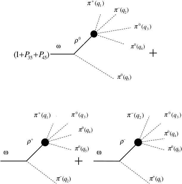
Figure 1: The diagrams describing the amplitudes of the decay $\omega\to\pi^{+}\pi^{-}3\pi^{0}$ through the $\rho$ intermediate state followed by the decay $\rho\to 4\pi$. The shaded circles refer to the whole $\rho\to 4\pi$ amplitudes.

where we explicitly label each particle in the reaction by its four-momentum, are shown in Fig. 1$-$4. Let us give the expressions corresponding to them. The upper index $(n)$ (pointing to neutral, because three neutral pions are in the final state) will designate this particular isotopic state. The amplitude corresponding to Fig. 1, includes the four pion decay of the intermediate $\rho$ meson which was extensively discussed in, e.g., ach00 . The Lagrangian due to Weinberg weinberg68 was used in Ref. ach00 to find the expressions for the $\rho\to 4\pi$ decay amplitudes. This Lagrangian is different in coefficients as compared to Eq. (5) above. However, one can show by direct computation that due to the well known parameter independence the $\rho\to 4\pi$ decay amplitudes resulting from the above Lagrangians coincide. The reason is that the terms $\propto D_{\pi}(k)$ in the $\pi\to 3\pi$ amplitudes,

$$M(\pi_{k}^{+}\to\pi^{+}_{q_{1}}\pi^{+}_{q_{2}}\pi^{-}_{q_{3}}) = {1\over 2f^{2}_{\pi}}(1+\hat{P}_{12})\left[-a(q_{1},q_{3})+(a-2)(q_{1},q_{2})+am^{2}_{\rho}{(q_{2},q_{3}-q_{1})\over D_{\rho}(q_{1}+q_{3})}-\right.$$

$$\left.{1\over 3}D_{\pi^{+}}(k)\right],$$

$$M(\pi_{k}^{+}\to\pi^{+}_{q_{1}}\pi^{0}_{q_{3}}\pi^{0}_{q_{4}}) = {1\over 2f^{2}_{\pi}}(1+\hat{P}_{34})\left[-(a-1)(q_{3},q_{4})+(a-2)(q_{1},q_{3})+am^{2}_{\rho}{(q_{4},q_{3}-q_{1})\over D_{\rho}(q_{1}+q_{3})}-\right.$$

$$\left.{1\over 6}D_{\pi^{+}}(k)\right],$$

$$M(\pi_{k}^{0}\to\pi^{+}_{q_{1}}\pi^{-}_{q_{2}}\pi^{0}_{q_{5}}) = {1\over 2f^{2}_{\pi}}(1+\hat{P}_{12})\left[-(a-1)(q_{1},q_{2})+(a-2)(q_{1},q_{5})+am^{2}_{\rho}{(q_{2},q_{1}-q_{5})\over D_{\rho}(q_{1}+q_{5})}-\right.$$

$$\left.{1\over 6}D_{\pi^{0}}(k)\right],$$

$$M(\pi^{0}\to\pi^{0}_{q_{3}}\pi^{0}_{q_{4}}\pi^{0}_{q_{5}}) = {m^{2}_{\pi^{0}}\over f^{2}_{\pi}},$$ (14)

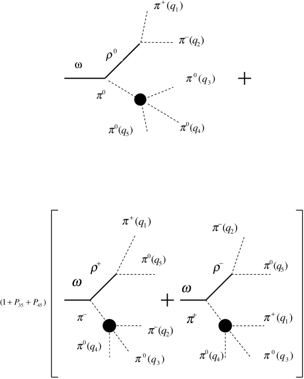
Figure 2: The diagrams describing the amplitudes of the decay $\omega\to\pi^{+}\pi^{-}3\pi^{0}$ through the $\rho\pi$ intermediate state followed by the transitions $\rho\to 2\pi$ and $\pi\to 3\pi$. The shaded circles refer to the effective $\pi\to 3\pi$ vertices given by Eq. (14). Note that non-$\pi$-pole term is included to the diagrams in Fig. 4 below.

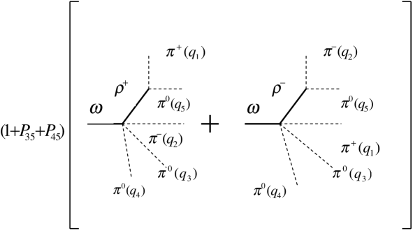
Figure 4: The contributions to the $\omega\to\pi^{+}\pi^{-}3\pi^{0}$ decay amplitude arising due to the chiral vertex $\omega\to\rho 3\pi$.

which vanish on the pion mass shell, give the non-$\pi$-pole terms in the $\rho\to 2\pi\to 4\pi$ amplitude. When added to the point like $\rho\to 4\pi$ amplitude, they make their sum parameter independent. The same occurs with such terms in the expression derived from Fig. 2 below, which should be added to the expression derived from Fig. 4. The final expressions for the full $\omega\to\pi^{+}\pi^{-}3\pi^{0}$ decay amplitude will be given below. Hereafter $\hat{P}_{ij}$ is the operator of permutation of the pion momenta $q_{i}$ and $q_{j}$,

$$D_{\rho}(k)=m^{2}_{\rho}-k^{2}-i\sqrt{k^{2}}\Gamma_{\rho\to\pi^{+}\pi^{-}}(k^{2}),$$

$$\Gamma_{\rho\to\pi^{+}\pi^{-}}(k^{2})={g^{2}_{\rho\pi\pi}\over 48\pi k^{2}}\left(k^{2}-4m^{2}_{\pi^{+}}\right)^{3/2}$$ (15)

are the inverse propagator of $\rho$ meson and its two pion decay width, respectively, and

$$D_{\pi^{+,0}}(k)=m^{2}_{\pi^{+,0}}-k^{2}$$ (16)

is the inverse propagator of $\pi^{\pm,0}$ meson. The following shorthand notations for inverse propagators of the particle $A$ will be used:

$$D_{Aab}\equiv D_{A}(q_{a}+q_{b})\mbox{, }D_{Aabc}\equiv D_{A}(q_{a}+q_{b}+q_{c}).$$ (17)

Let us give the expression for each diagram in Fig. 1$-$5. Choosing $q_{\mu}\mbox{, }\epsilon_{\mu}$ for the four-momentum and four-vector of polarization of the $\omega$, one obtains

$$M^{(n)}_{1} = {g_{\omega\rho\pi}g_{\rho\pi\pi}\over f^{2}_{\pi}}\varepsilon_{\mu\nu\lambda\sigma}q_{\mu}\epsilon_{\nu}\left[\left(1+\hat{P}_{35}+\hat{P}_{45}\right){q_{5\lambda}\over D_{\rho}(q-q_{5})}J_{\sigma}(\rho^{0}\to\pi^{+}_{q_{1}}\pi^{-}_{q_{2}}\pi^{0}_{q_{3}}\pi^{0}_{q_{4}})+\right.$$ (18)

$$\left.(1-\hat{P}_{12}){q_{2\lambda}\over D_{\rho}(q-q_{2})}J_{\sigma}(\rho^{+}\to\pi^{+}_{q_{1}}\pi^{0}_{q_{3}}\pi^{0}_{q_{4}}\pi^{0}_{q_{5}})\right]$$

for the diagram Fig. 1. The $\rho\to 4\pi$ decay currents standing in Eq. (18) are ach00

$$J_{\sigma}(\rho^{0}\to\pi^{+}_{q_{1}}\pi^{-}_{q_{2}}\pi^{0}_{q_{3}}\pi^{0}_{q_{4}}) = (1-\hat{P}_{12})(1+\hat{P}_{34})\left\{q_{1\sigma}\left(-{1\over 4}+{1\over D_{\pi^{+}234}}\left[(q_{3},q_{4}-2q_{2})+a\times\right.\right.\right.$$ (19)

$$\left.\left.\left.(q_{3},q_{2}-q_{4})\left({m^{2}_{\rho}\over D_{\rho 24}}-1\right)\right]\right)+{m^{2}_{\rho}\over 2D_{\rho 13}D_{\rho 24}}\left[(q_{3}+q_{1})_{\sigma}\times\right.\right.$$

$$\left.\left.(q_{1}-q_{3},q_{2}-q_{4})+2(q_{3}-q_{1})_{\sigma}(q_{1}+q_{3},q_{2}-q_{4})\right]+\right.$$

$$\left.2\left({n_{c}g^{2}c_{3}\over 8\pi^{2}}\right)^{2}{1\over D_{\omega 123}}\left({1\over D_{\rho 12}}+{1\over D_{\rho 13}}+{1\over D_{\rho 23}}+3{c_{1}-c_{2}-c_{3}\over 2c_{3}m^{2}_{\rho}}\right)\times\right.$$

$$\left.\left[q_{1\sigma}\left((k,q_{2})(q_{3},q_{4})-(k,q_{3})(q_{2},q_{4})\right)+q_{3\sigma}(k,q_{1})(q_{2},q_{4})\right]\right\},$$

(with $k=q_{1}+q_{2}+q_{3}+q_{4}$), where

$$D_{\omega abc}\equiv D_{\omega}(q_{a}+q_{b}+q_{c})=m^{2}_{\omega}-(q_{a}+q_{b}+q_{c})^{2}-im_{\omega}\Gamma_{\omega}$$ (20)

is the inverse propagator of the $\omega$ (we take the fixed width approximation for $\omega$ meson because the $\omega$ resonance is narrow), and

$$J_{\sigma}(\rho^{+}\to\pi^{+}_{q_{1}}\pi^{0}_{q_{3}}\pi^{0}_{q_{4}}\pi^{0}_{q_{5}}) = (1+\hat{P}_{34}+\hat{P}_{35})\left\{{1\over 3}q_{1\sigma}\left(1-{2m^{2}_{\pi^{0}}\over D_{\pi^{0}345}}\right)+{q_{3\sigma}\over D_{\pi^{+}145}}(1+\hat{P}_{45})\times\right.$$ (21)

$$\left.\left[(q_{4},q_{5}-2q_{1})+a(q_{4},q_{5}-q_{1})\left({m^{2}_{\rho}\over D_{\rho 15}}-1\right)\right]\right\}.$$

The expression for the diagrams in Fig. 2 is

$$M^{(n)}_{2} = -{g_{\omega\rho\pi}g_{\rho\pi\pi}\over f^{2}_{\pi}}(1-\hat{P}_{12})(1+\hat{P}_{35}+\hat{P}_{45})(1+\hat{P}_{34})\varepsilon_{\mu\nu\lambda\sigma}q_{\mu}\epsilon_{\nu}\times$$ (22)

$$\left\{{q_{1\lambda}q_{5\sigma}\over D_{\rho 15}D_{\pi^{+}234}}\left[(q_{3},q_{4}-2q_{2})+a(q_{3},q_{2}-q_{4})\left({m^{2}_{\rho}\over D_{\rho 24}}-1\right)\right]-{q_{1\lambda}q_{2\sigma}m^{2}_{\pi^{0}}\over 6D_{\rho 12}D_{\pi^{0}345}}\right\}.$$

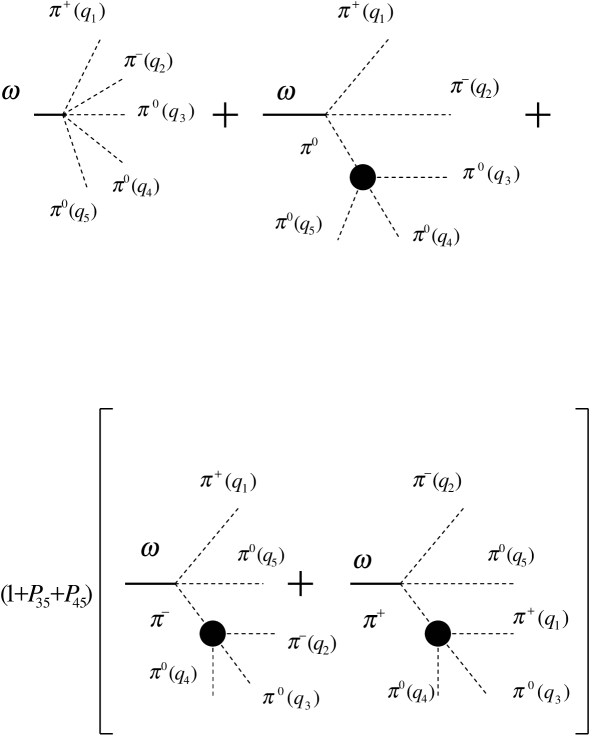
Figure 3: The diagrams describing the contributions to the $\omega\to\pi^{+}\pi^{-}3\pi^{0}$ decay amplitude via point like vertices. The shaded circles refer to the effective $\pi\to 3\pi$ vertices given by Eq. (14).

The expression for the diagram Fig. 3 is

$$M^{(n)}_{3} = {n_{c}g\over 32\pi^{2}f^{5}_{\pi}}(1-\hat{P}_{12})(1+\hat{P}_{35}+\hat{P}_{45})\varepsilon_{\mu\nu\lambda\sigma}q_{\mu}\epsilon_{\nu}\left\{{4c_{1}-5(c_{2}+c_{3})\over 3}q_{1\lambda}q_{2\sigma}+\right.$$ (23)

$$\left.3(c_{1}-c_{2}-c_{3})(1+\hat{P}_{34})\left[{q_{1\lambda}q_{5\sigma}\over D_{\pi^{+}234}}\left((q_{3},q_{4}-2q_{2})+a(q_{3},q_{2}-q_{4})\left({m^{2}_{\rho}\over D_{\rho 24}}-1\right)\right)+\right.\right.$$

$$\left.\left.{q_{1\lambda}q_{2\sigma}\over 3D_{\pi^{0}345}}(q_{3},q_{4})\right]\right\}.$$

Notice the relation

$${n_{c}g\over 32\pi^{2}f^{5}_{\pi}}=-{g_{\omega\rho\pi}g_{\rho\pi\pi}\over f^{2}_{\pi}}\cdot{1\over 2c_{3}m^{2}_{\rho}}$$ (24)

which is useful for an easier comparison of the present contribution with others. The expression for the diagrams Fig. 4 and 5 are, respectively,

$$M^{(n)}_{4} = -{g_{\omega\rho\pi}g_{\rho\pi\pi}\over f^{2}_{\pi}}(1-\hat{P}_{12})(1+\hat{P}_{35}+\hat{P}_{45})\varepsilon_{\mu\nu\lambda\sigma}{\epsilon_{\nu}(q_{1}-q_{5})_{\lambda}\over 2D_{\rho 15}}\times$$ (25)

$$\left[q_{\mu}q_{2\sigma}-{c_{1}+c_{2}-c_{3}\over 2c_{3}}q_{2\mu}(q_{3}+q_{4})_{\sigma}\right],$$

and

$$M^{(n)}_{5}={g_{\omega\rho\pi}g_{\rho\pi\pi}m^{2}_{\rho}\over f^{2}_{\pi}}\cdot{c_{1}+c_{2}-c_{3}\over 4c_{3}}(1-\hat{P}_{12})(1+\hat{P}_{35}+\hat{P}_{45})\varepsilon_{\mu\nu\lambda\sigma}{\epsilon_{\nu}(q_{1}-q_{3})_{\mu}(q_{2}-q_{4})_{\lambda}q_{5\sigma}\over D_{\rho 13}D_{\rho 24}}.$$ (26)

The full $\omega\to\pi^{+}\pi^{-}3\pi^{0}$ decay amplitude is

$$M(\omega_{q}\to\pi^{+}_{q_{1}}\pi^{-}_{q_{2}}\pi^{0}_{q_{3}}\pi^{0}_{q_{4}}\pi^{0}_{q_{5}})=M^{(n)}_{1}+M^{(n)}_{2}+M^{(n)}_{3}+M^{(n)}_{4}+M^{(n)}_{5}.$$ (27)

Since the expression for the amplitude is very cumbersome, one should invoke the method of the control of the calculations. We take the Adler condition as the method of such a control.

II.1.1 Verifying the Adler condition for the $\omega\to\pi^{+}\pi^{-}3\pi^{0}$ decay amplitude

The Adler condition is the condition of vanishing of the amplitude of the process with soft pions when the four-momentum of any pion is vanishing. Pions emitted in the decay $\omega\to 5\pi$ ach00 are truly soft, because they possess the typical momentum $|{\bf q}_{\pi}|\simeq 0.5m_{\pi}$. To verify the Adler condition, we set any particular pion momentum to zero. The correct expression for the amplitude should then vanish.

i) $q_{1}=0$. The contributions of the diagrams Fig. 3, 4, 5 vanish, the contributions of the diagrams Fig. 1 and 2 are equal in magnitude but opposite in sign, hence they are cancelled. The Adler condition is fulfilled. The case $q_{2}=0$ is obtained from the case of $q_{1}=0$ by the permutation property, see the operator $1-\hat{P}_{12}$ in front of each expression in Eq. (18), (19), (22), (23), (25) and (26).

ii) $q_{3}=0$. Here the situation is more subtle. Let us represent the amplitude at $q_{3}=0$ in the form

$$M^{(n)}(q_{3}=0)=-{g_{\omega\rho\pi}g_{\rho\pi\pi}\over f^{2}_{\pi}}(1-\hat{P}_{12})(1+\hat{P}_{45})\epsilon_{\mu\nu\lambda\sigma}\epsilon_{\nu}T_{\mu\lambda\sigma}.$$

Then one obtains the following contributions to the tensor $T_{\mu\lambda\sigma}$ from the diagrams Fig. 1$-$5, respectively:

$$T_{\mu\lambda\sigma}^{(1)} = {q_{\mu}(q_{1}-q_{4})_{\lambda}q_{5\sigma}\over 2D_{\rho 14}},$$

$$T_{\mu\lambda\sigma}^{(2)} = {q_{\mu}q_{1\lambda}q_{4\sigma}\over D_{\rho 14}},$$

$$T_{\mu\lambda\sigma}^{(3)} = -{1\over 4m^{2}_{\rho}}\left(q_{\mu}q_{1\lambda}q_{2\sigma}+{c_{1}+c_{2}-c_{3}\over c_{3}}\cdot q_{1\mu}q_{2\lambda}q_{4\sigma}\right),$$

$$T_{\mu\lambda\sigma}^{(4)} = {1\over 6}q_{\mu}\left[{3q_{1\lambda}q_{2\sigma}\over 2m^{2}_{\rho}}+{(q_{1}-q_{4})_{\lambda}(2q_{2}-q_{5})_{\sigma}-2q_{1\lambda}q_{4\sigma}\over D_{\rho 14}}\right]-$$

$${c_{1}+c_{2}-c_{3}\over 4c_{3}}\left[{q_{2\mu}(q_{1}-q_{4})_{\lambda}q_{5\sigma}\over D_{\rho 14}}-{q_{1\mu}q_{2\lambda}q_{4\sigma}\over m^{2}_{\rho}}\right],$$

$$T_{\mu\lambda\sigma}^{(5)} = {c_{1}+c_{2}-c_{3}\over 4c_{3}}\cdot{q_{2\mu}(q_{1}-q_{4})_{\lambda}q_{5\sigma}\over D_{\rho 14}}.$$ (28)

In the above formulas, the upper index points to the label of the corresponding figure. Note that when obtaining the contribution $T^{(3)}_{\mu\lambda\sigma}$, the relation Eq. (24) is essential. As is seen from Eq. (28), the terms with the factor $(c_{1}+c_{2}-c_{3})$ and without such a factor are cancelled separately in the sum. Let us check this for the terms $\propto q_{\mu}/6D_{\rho 14}$. One has for the sum of these terms $2(q_{1}-q_{4})_{\lambda}(q_{2}+q_{5})_{\sigma}+4q_{1\lambda}q_{4\sigma}$. Using the four-momentum conservation and taking into account the tensor $\epsilon_{\mu\nu\lambda\sigma}$, one can see that the above momentum combination vanishes. Hence, the Adler condition is satisfied in the case $q_{3}=0$, too. The cases $q_{4,5}=0$ are obtained from this case by Bose symmetry.

II.2 The $\omega\to 2\pi^{+}2\pi^{-}\pi^{0}$ final state

The diagrams for the amplitude of the decay

$$\omega_{q}\to\pi^{+}_{q_{1}}\pi^{+}_{q_{2}}\pi^{-}_{q_{3}}\pi^{-}_{q_{4}}\pi^{0}_{q_{5}},$$ (29)

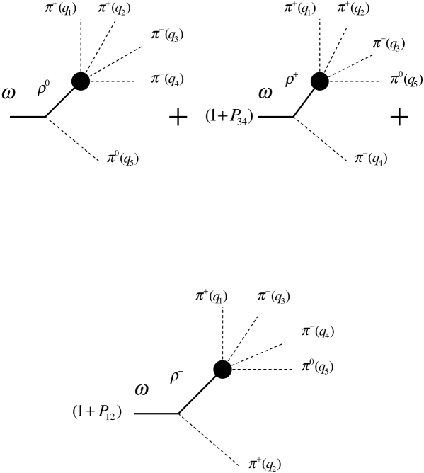
Figure 6: The diagrams describing the amplitudes of the decay $\omega\to 2\pi^{+}2\pi^{-}\pi^{0}$ through the $\rho$ intermediate state followed by the decay $\rho\to 4\pi$. The shaded circles refer to the whole $\rho\to 4\pi$ amplitudes.

where the particles are labeled by their four-momenta, are shown in Fig. 6$-$10. Let us give the expressions corresponding to them. The upper index $(c)$ (denoting charged, because most pions in final state are charged) will designate this particular isotopic state. The expression for the diagram Fig. 6 looks as

$$M^{(c)}_{1} = {g_{\omega\rho\pi}g_{\rho\pi\pi}\over f^{2}_{\pi}}\varepsilon_{\mu\nu\lambda\sigma}q_{\mu}\epsilon_{\nu}\left[{q_{5\lambda}\over D_{\rho}(q-q_{5})}J_{\sigma}(\rho^{0}\to\pi^{+}_{q_{1}}\pi^{+}_{q_{2}}\pi^{-}_{q_{3}}\pi^{-}_{q_{4}})+\right.$$ (30)

$$\left.(1+\hat{P}_{34}){q_{4\lambda}\over D_{\rho}(q-q_{4})}J_{\sigma}(\rho^{+}\to\pi^{+}_{q_{1}}\pi^{+}_{q_{2}}\pi^{-}_{q_{3}}\pi^{0}_{q_{5}})+\right.$$

$$\left.(1+\hat{P}_{12}){q_{2\lambda}\over D_{\rho}(q-q_{2})}J_{\sigma}(\rho^{-}\to\pi^{+}_{q_{1}}\pi^{-}_{q_{3}}\pi^{-}_{q_{4}}\pi^{0}_{q_{5}})\right].$$

Here the currents responsible for the four pion decay of intermediate $\rho$ meson are the following ach00 :

$$J_{\sigma}(\rho^{0}\to\pi^{+}_{q_{1}}\pi^{+}_{q_{2}}\pi^{-}_{q_{3}}\pi^{-}_{q_{4}}) = (1+\hat{P}_{12})(1+\hat{P}_{34})(1-\hat{P}_{13}\hat{P}_{24})\left\{q_{1\sigma}\left(-{1\over 2}+{1\over D_{\pi^{+}234}}\times\right.\right.$$ (31)

$$\left.\left.\left[a(q_{3},q_{2}-q_{4})\left({m^{2}_{\rho}\over D_{\rho 24}}-1\right)-2(q_{3},q_{4})\right]\right)\right\};$$

and

$$J_{\sigma}(\rho^{+}\to\pi^{+}_{q_{1}}\pi^{+}_{q_{2}}\pi^{-}_{q_{3}}\pi^{0}_{q_{5}}) = (1+\hat{P}_{12})\left\{{1\over 2}(q_{1}-q_{5})_{\sigma}-(1+\hat{P}_{23}){q_{1\sigma}\over D_{\pi^{0}135}}\left[(q_{2},q_{3}-2q_{5})+\right.\right.$$ (32)

$$\left.\left.a(q_{2},q_{3}-q_{5})\left({m^{2}_{\rho}\over D_{\rho 35}}-1\right)\right]+{q_{5\sigma}\over D_{\pi^{+}123}}\left[-2(q_{1},q_{2})+a(q_{1},q_{3}-q_{2})\times\right.\right.$$

$$\left.\left.\left({m^{2}_{\rho}\over D_{\rho 23}}-1\right)\right]+(1-\hat{P}_{35})\left[2(q_{1}-q_{5})_{\sigma}(q_{1}+q_{5},q_{2}-q_{3})-\right.\right.$$

$$\left.\left.(q_{1}+q_{5})_{\sigma}(q_{1}-q_{5},q_{2}-q_{3})\right]{m^{2}_{\rho}\over 2D_{\rho 15}D_{\rho 23}}+{2\over D_{\omega 135}}\left({n_{c}g^{2}c_{3}\over 8\pi^{2}}\right)^{2}\times\right.$$

$$\left.\left[q_{1\sigma}(1-\hat{P}_{35})(k,q_{3})(q_{2},q_{5})+q_{3\sigma}(1-\hat{P}_{15})(k,q_{5})(q_{1},q_{2})+\right.\right.$$

$$\left.\left.q_{5\sigma}(1-\hat{P}_{13})(k,q_{1})(q_{2},q_{3})\right]\left({1\over D_{\rho 13}}+{1\over D_{\rho 15}}+{1\over D_{\rho 33}}+\right.\right.$$

$$\left.\left.{c_{1}-c_{2}-c_{3}\over 2c_{3}m^{2}_{\rho}}\right)\right\},$$

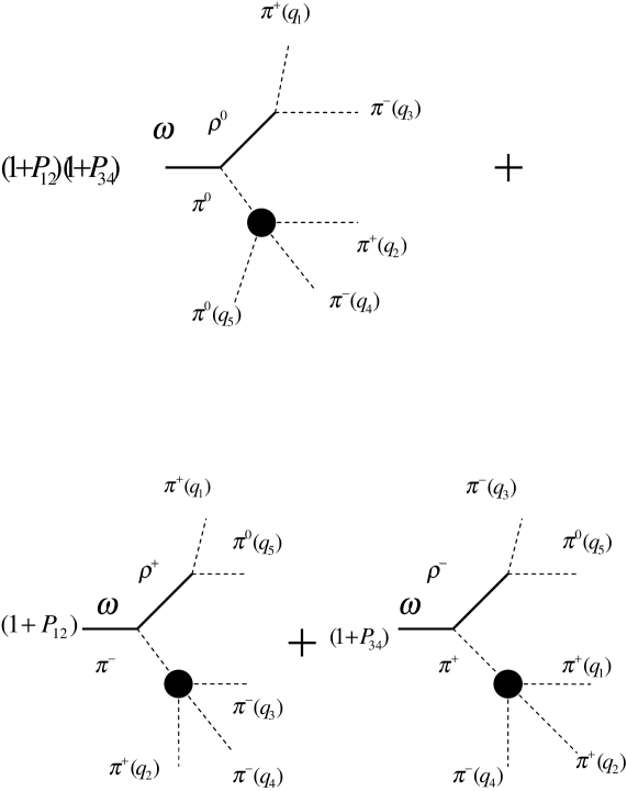
Figure 7: The diagrams describing the amplitudes of the decay $\omega\to 2\pi^{+}2\pi^{-}\pi^{0}$ through the $\rho\pi$ intermediate state followed by the transitions $\rho\to 2\pi$ and $\pi\to 3\pi$. The shaded circles refer to the effective $\pi\to 3\pi$ vertices given by Eq. (14). Note that non-$\pi$-pole term is included to the first pair of diagrams in Fig. 9 below.

where $k=q_{1}+q_{2}+q_{3}+q_{5}$. The expression for $J_{\sigma}(\rho^{-}\to\pi^{+}_{q_{1}}\pi^{-}_{q_{3}}\pi^{-}_{q_{4}}\pi^{0}_{q_{5}})$ is obtained from Eq. (32) by the replacements $q_{1}\leftrightarrow q_{3}$, $q_{2}\to q_{4}$ and by inverting an overall sign. The expression for the contribution of the diagrams Fig. 7 is

$$M^{(c)}_{2} = {g_{\omega\rho\pi}g_{\rho\pi\pi}\over f^{2}_{\pi}}(1+\hat{P}_{12})(1+\hat{P}_{34})\varepsilon_{\mu\nu\lambda\sigma}q_{\mu}\epsilon_{\nu}\left\{(1+\hat{P}_{24}){q_{1\lambda}q_{3\sigma}\over D_{\rho 13}D_{\pi^{0}245}}\times\right.$$ (33)

$$\left.\left[(q_{2},q_{4}-2q_{5})+a(q_{2},q_{4}-q_{5})\left({m^{2}_{\rho}\over D_{\rho 45}}-1\right)\right]-(1-\hat{P}_{13}\hat{P}_{24})\times\right.$$

$$\left.{q_{1\lambda}q_{5\sigma}\over D_{\rho 15}D_{\pi^{+}234}}\left[-2(q_{3},q_{4})+a(q_{3},q_{2}-q_{4})\left({m^{2}_{\rho}\over D_{\rho 24}}-1\right)\right]\right\}.$$

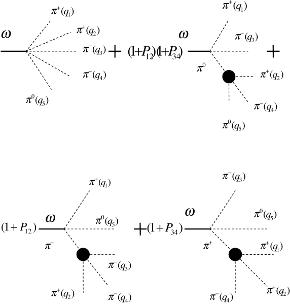
Figure 8: The diagrams describing the contributions to the $\omega\to 2\pi^{+}2\pi^{-}\pi^{0}$ decay amplitude via point like vertices. The shaded circles refer to the effective $\pi\to 3\pi$ vertices given by Eq. (14).

The expression for the contribution of the diagrams Fig. 8 looks as

$$M^{(c)}_{3} = {n_{c}g\over 32\pi^{2}f^{5}_{\pi}}(1+\hat{P}_{12})(1+\hat{P}_{34})\varepsilon_{\mu\nu\lambda\sigma}q_{\mu}\epsilon_{\nu}\left\{{4c_{1}-5(c_{2}+c_{3})\over 3}\cdot q_{1\lambda}q_{3\sigma}+\right.$$ (34)

$$\left.3(c_{1}-c_{2}-c_{3})\left((1-\hat{P}_{14}\hat{P}_{23}){q_{1\lambda}q_{5\sigma}\over D_{\pi^{+}234}}\left[-2(q_{3},q_{4})+a(q_{3},q_{2}-q_{4})\times\right.\right.\right.$$

$$\left.\left.\left.\left({m^{2}_{\rho}\over D_{\rho 24}}-1\right)\right]-{q_{1\lambda}q_{3\sigma}\over D_{\pi^{0}245}}(1+\hat{P}_{24})\left[(q_{2},q_{4}-2q_{5})+a(q_{2},q_{4}-q_{5})\times\right.\right.\right.$$

$$\left.\left.\left.\left({m^{2}_{\rho}\over D_{\rho 45}}-1\right)\right]\right)\right\}.$$

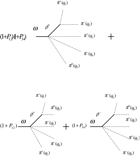
Figure 9: The contributions to the $\omega\to 2\pi^{+}2\pi^{-}\pi^{0}$ decay amplitude arising due to the chiral $\omega\to\rho 3\pi$ vertex.

Again, the relation Eq. (24) is necessary in verifying the Adler condition below. The expression for the contribution of the diagram Fig. 9 is

$$M^{(c)}_{4} = {g_{\omega\rho\pi}g_{\rho\pi\pi}\over f^{2}_{\pi}}(1+\hat{P}_{12})(1+\hat{P}_{34})\varepsilon_{\mu\nu\lambda\sigma}\epsilon_{\nu}\left\{{1\over 2}q_{\mu}\left[{(q_{1}-q_{3})_{\lambda}q_{5\sigma}\over D_{\rho 13}}+(1-\hat{P}_{13}\hat{P}_{24})\times\right.\right.$$ (35)

$$\left.\left.{q_{1\lambda}q_{5\sigma}+{1\over 2}(q_{1}-q_{5})_{\lambda}q_{2\sigma}\over D_{\rho 15}}\right]-{c_{1}+c_{2}-c_{3}\over 4c_{3}}\left[{q_{5\mu}(q_{1}-q_{3})_{\lambda}(q_{2}+q_{4})_{\sigma}\over D_{\rho 13}}+\right.\right.$$

$$\left.\left.(1-\hat{P}_{13}\hat{P}_{24}){q_{1\mu}(q_{3}-q_{5})_{\lambda}q_{4\sigma}\over D_{\rho 35}}\right]\right\}.$$

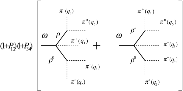
Figure 10: The contributions to the $\omega\to 2\pi^{+}2\pi^{-}\pi^{0}$ decay amplitude via intermediate state with two $\rho$ mesons.

Finally, the amplitude resulting from the diagram Fig. 10 is

$$M^{(c)}_{5} = -{g_{\omega\rho\pi}g_{\rho\pi\pi}m^{2}_{\rho}\over f^{2}_{\pi}}\cdot\left({c_{1}+c_{2}-c_{3}\over 4c_{3}}\right)(1+\hat{P}_{12})(1+\hat{P}_{34})(1+\hat{P}_{24})\times$$ (36)

$$\varepsilon_{\mu\nu\lambda\sigma}\epsilon_{\nu}{(q_{1}-q_{3})_{\mu}q_{4\lambda}(q_{2}-q_{5})_{\sigma}\over D_{\rho 13}D_{\rho 25}}.$$

Notice that the product of the operators $(1+\hat{P}_{12})(1+\hat{P}_{34})$ makes evident the Bose symmetry of the full $\omega\to 2\pi^{+}2\pi^{-}\pi^{0}$ decay amplitude,

$$M(\omega_{q}\to\pi^{+}_{q_{1}}\pi^{+}_{q_{2}}\pi^{-}_{q_{3}}\pi^{-}_{q_{4}}\pi^{0}_{q_{5}})=M^{(c)}_{1}+M^{(c)}_{2}+M^{(c)}_{3}+M^{(c)}_{4}+M^{(c)}_{5}.$$ (37)

II.2.1 Verifying the Adler condition for the $\omega\to 2\pi^{+}2\pi^{-}\pi^{0}$ decay amplitude

Let us write down the Adler limits of all the above contributions to the $\omega\to 2\pi^{+}2\pi^{-}\pi^{0}$ decay amplitudes. As an example, the case $q_{1}=0$ is considered in detail. Representing the total amplitude Eq. (37) in this limit as

$$M^{(c)}(q_{1}=0)={g_{\omega\rho\pi}g_{\rho\pi\pi}\over f^{2}_{\pi}}(1+\hat{P}_{34})\varepsilon_{\mu\nu\lambda\sigma}\epsilon_{\nu}T_{\mu\lambda\sigma},$$

one has the following expressions for the diagrams Fig. 6$-$10, respectively,

$$T^{(6)}_{\mu\lambda\sigma}(q_{1}=0) = {1\over 2}(1-\hat{P}_{35})q_{\mu}\left[{q_{4\lambda}(q_{2}-q_{5})_{\sigma}\over D_{\rho 25}}+{q_{2\lambda}q_{3\sigma}\over D_{\rho 35}}\right],$$

$$T^{(7)}_{\mu\lambda\sigma}(q_{1}=0) = (1-\hat{P}_{35}){q_{\mu}q_{2\lambda}q_{3\sigma}\over D_{\rho 23}},$$

$$T^{(8)}_{\mu\lambda\sigma}(q_{1}=0) = -\left(2+{c_{1}+c_{2}-c_{3}\over c_{3}}\right){q_{\mu}q_{2\lambda}q_{5\sigma}\over 4m^{2}_{\rho}},$$

$$T^{(9)}_{\mu\lambda\sigma}(q_{1}=0) = {1\over 6}q_{\mu}\left[{-2q_{2\lambda}q_{3\sigma}+(q_{2}-q_{3})_{\lambda}(2q_{5}-q_{4})_{\sigma}\over D_{\rho 35}}-\right.$$

$$\left.{4q_{3\lambda}q_{5\sigma}+(q_{3}-q_{5})_{\lambda}(2q_{4}-q_{2})_{\sigma}\over D_{\rho 23}}+q_{2\lambda}q_{5\sigma}\left({3\over D_{\rho 25}}+{3\over m^{2}_{\rho}}\right)\right]+$$

$${c_{1}+c_{2}-c_{3}\over 4c_{3}}\left[{q_{\mu}q_{2\lambda}q_{5\sigma}\over m^{2}_{\rho}}+(1-\hat{P}_{24}\hat{P}_{35}){q_{3\mu}(q_{4}-q_{5})_{\lambda}q_{2\sigma}\over D_{\rho 45}}\right],$$

$$T^{(10)}_{\mu\lambda\sigma}(q_{1}=0) = -{c_{1}+c_{2}-c_{3}\over 4c_{3}}(1-\hat{P}_{24}\hat{P}_{35}){q_{3\mu}(q_{4}-q_{5})_{\lambda}q_{2\sigma}\over D_{\rho 45}}.$$ (38)

In the above formulas, the upper index points to the label of the corresponding figure. Once again, when obtaining $T^{(8)}_{\mu\lambda\sigma}$, the relation (24) is essential. The close inspection of Eq. (38) shows that the sum of above tensors vanishes. Indeed, the cancellation of the $\rho$ pole terms proportional to $c_{1}+c_{2}-c_{3}$ and of all the non-$\rho$-pole terms is evident. Let us check the cancellation of the $\rho$ pole terms taking as an example the terms $\propto q_{\mu}/6D_{\rho 25}$. One has for the sum of such terms the expression $3[q_{4\lambda}(q_{2}-q_{5})_{\sigma}-q_{2\lambda}q_{5\sigma}]$. Applying the operator $1+\hat{P}_{34}$, taking into account the four-momentum conservation and the presence of the tensor $\epsilon_{\mu\nu\lambda\sigma}$ one finds that the above combination vanishes. The cancellation of the remaining $\rho$ pole terms is checked in the same manner. The cases of $q_{2,3,4}=0$ are obtained from the present case by Bose symmetry and by the evident replacements of the pion momenta. In the case $q_{5}=0$, the contributions of the diagrams Fig. 8, 9, and 10 vanish separately, while the contributions of the diagrams Fig. 6 and 7 are equal in magnitude but opposite in sign, hence they are cancelled. The conditions of the vanishing of the amplitude in the Adler limit obtained in subsection II.1.1 and this subsection turn out to be of great importance in obtaining the $\phi\to 5\pi$ decay amplitudes.

III The $\omega\to\pi^{+}\pi^{-}3\pi^{0}$ and $\omega\to 2\pi^{+}2\pi^{-}\pi^{0}$ branching ratios revisited.

In our previous work Ref. ach00 , the branching ratios of the $\omega\to\pi^{+}\pi^{-}3\pi^{0}$ and $\omega\to 2\pi^{+}\pi^{-}\pi^{0}$ decays were estimated. Essential for that evaluation were the expressions for the contributions of the diagrams shown in Fig. 1 and 6, added with the specific correction factor stemming from the diagrams shown in Fig. 2 and 7 of the present paper, respectively. This seemed to be justifiable because of the presence of the $\rho$ pole. As it will become clear later on, the non-$\rho$-pole terms are essential.

Strictly speaking, the HLS approach does not give the predictions even for the $\omega\to\pi^{+}\pi^{-}\pi^{0}$ decay rate, because arbitrary constants $c_{1,2,3}$ enter the expression for Lagrangian Eq. (9). As was pointed out in Ref. hls1 ; hls2 , these constants should be determined from experiment. Nevertheless, HLS relates the contributions to the amplitudes, compare Fig. 1, 2 to Fig. 3, 4, and 5 (respectively, Fig. 6, 7 to Fig. 8, 9, and 10), which otherwise appear unrelated. One can obtain reasonable predictions for the $\omega\to 5\pi$ decay rates upon assuming particular relations among $c_{1,2,3}$. First, there are no experimental indications on the point like $\omega\to\pi^{+}\pi^{-}\pi^{0}$ vertex, hence one can take the relation Eq. (11) for granted. Second, the constant $c_{3}$, see Eq. (12), extracted from the $\omega\to 3\pi$ branching ratio, is remarkably close to unity. Note that older chiral models schechter for the vector mesons interactions, added with the terms arising from the gauging the anomalous Wess-Zumino action wza , predicted $c_{3}=1$. We fix $c_{3}$ from the $\omega\to 3\pi$ partial width, see Eq. (10) and (12). After taking into account Eq. (11), the ratio $c_{1}/c_{3}$ remains arbitrary, and the magnitude of the $\omega\to 5\pi$ decay width depends on this parameter. We choose its value guided by the following considerations. The inspection of the expressions for the $\omega\to 5\pi$ decay amplitudes obtained in Sec. II shows that almost all the terms except those proportional to $c_{1}+c_{2}-c_{3}$, has the tensor structure

$$M={g_{\omega\rho\pi}g_{\rho\pi\pi}\over f^{2}_{\pi}}\varepsilon_{\mu\nu\lambda\sigma}q_{\mu}\epsilon_{\nu}T_{\lambda\sigma},$$ (39)

where

$$T_{\lambda\sigma}=\sum_{a<b}G_{ab}q_{(a)\lambda}q_{(b)\sigma}$$ (40)

is the tensor composed of pion four-momenta $q_{(a)}$, $a=1,...5$, and $G_{ab}$ are invariant amplitudes, whose explicit form can be read off the expressions for the amplitudes obtained in Sec. II by gathering the coefficients in front of $q_{(a)\lambda}q_{(b)\sigma}$. They are very lengthy, so we do not give them here. In the rest frame system of the decaying $\omega$, the Lorentz structure of Eq. (39) is reduced to the three dimensional form $e_{ijk}\xi_{i}T_{jk}$, where $\bm{\xi}$ is the polarization vector of the $\omega$ in this frame, $e_{ijk}$ is totally antisymmetric in $i,j,k=1,2,3$. This enormously simplify the calculation of the modulus squared of the amplitude. In the meantime, the terms proportional to $c_{1}+c_{2}-c_{3}$ has entirely the four dimensional tensor structure $\varepsilon_{\mu\nu\lambda\sigma}\epsilon_{\mu}q_{(a)\nu}q_{(b)\lambda}q_{(c)\sigma}$. The resulting expression for the modulus squared of the full amplitude turns out to be extremely lengthy. For the sake of simplicity, we set

$$c_{1}+c_{2}-c_{3}=0$$ (41)

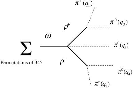
Figure 5: The contributions to the $\omega\to\pi^{+}\pi^{-}3\pi^{0}$ decay amplitude via intermediate state with two $\rho$ mesons. Total number of diagrams of this kind is $3!=6$.

in what follows. Note that this means that the contributions of the diagrams Fig. 5, 10 together with the part of the contributions from the diagrams Fig. 4 and 9 are dropped. The results of relaxing the condition Eq. (41) are discussed at the end of the present Section. Finally, our assumptions about HLS arbitrary constants $c_{1,2,3}$ and $a$ are

$$c_{1}=c_{3}\mbox{, }c_{2}=0\mbox{, }a=2.$$ (42)

Notice that the above relations among $c_{1,2,3}$ are the solutions of Eq. (11) and (41).

The expression for the partial width of the decays (1) and (2) looks as

$$\Gamma_{\omega\to 5\pi}(s)={1\over 2\sqrt{s}(2\pi)^{11}N_{\rm sym}}\int|M|^{2}d{\cal D}_{5},$$ (43)

where $s=\left(\sum_{a=1}^{5}q_{a}\right)^{2}$ is the total energy squared in the rest frame system of the decaying particle, the Bose symmetry factor $N_{\rm sym}=6\mbox{, }4$ for the reaction (1) and (2), respectively, and $d{\cal D}_{5}$ given in Ref. kumar is the differential element of the phase space volume of the five pion final state. Note that we take into account the mass difference of the charged and neutral pions both in amplitude and in the phase space volume. In the above formula,

$$|M|^{2}={1\over 3}\left({g_{\omega\rho\pi}g_{\rho\pi\pi}\over f^{2}_{\pi}}\right)^{2}{s\over 2}\sum_{i,j=1}^{3}|T_{ij}-T_{ji}|^{2}$$ (44)

is the modulus squared of the amplitude Eq. (39) averaged over three independent polarizations of the $\omega$. When evaluating Eq. (43), eight Mandelstam-like invariant variables $s_{i}$, $u_{i}$, $i=1,2,3$, and $t_{1}$, $t_{2}$ proposed by Kumar in Ref. kumar are suitable. They are given in Appendix. All the scalar products of the pair of pion four-momenta are expressed via the Kumar variables by the expressions given in Appendix. For the numerical evaluation of the eight dimensional integral over Kumar variables we use the method suggested in Ref. sag .

We evaluate both the branching ratios for the two mentioned isotopic modes at the resonance mass,

$$B_{\omega\to 5\pi}(m^{2}_{\omega})={\Gamma_{\omega\to 5\pi}(m^{2}_{\omega})\over\Gamma_{\omega}},$$ (45)

and the branching ratios averaged over resonance peak,

$$B^{\rm aver}_{\omega\to 5\pi}={2\over\pi}\int_{\sqrt{s}=m_{\omega}-\Gamma_{\omega}}^{\sqrt{s}=m_{\omega}+\Gamma_{\omega}}d\sqrt{s}{s\Gamma_{\omega\to 5\pi}(s)\over(s-m^{2}_{\omega})^{2}+m^{2}_{\omega}\Gamma^{2}_{\omega}}.$$ (46)

The quantity $B^{\rm aver}_{\omega\to 5\pi}$ is useful in situations where the total energy of the five pion state is not directly measured, as is the case in, e.g., photoproduction or peripheral production in $\pi N$ collisions. The results of the evaluation are the following:

$$B_{\omega\to\pi^{+}\pi^{-}3\pi^{0}}(m^{2}_{\omega}) = 3.6\times 10^{-9}\mbox{, }B^{\rm aver}_{\omega\to\pi^{+}\pi^{-}3\pi^{0}}=2.8\times 10^{-9},$$

$$B_{\omega\to 2\pi^{+}2\pi^{-}\pi^{0}}(m^{2}_{\omega}) = 3.5\times 10^{-9}\mbox{, }B^{\rm aver}_{\omega\to 2\pi^{+}2\pi^{-}\pi^{0}}=2.7\times 10^{-9}.$$ (47)

These branching ratios for the $\omega\to 5\pi$ decay by the factor of more than three exceed those obtained in our previous paper Ref. ach00 . The reason of the disagreement is the following. As is mentioned in the beginning of the present Section, the diagrams Fig. 1 and 6 corrected with those of Fig. 2 and 7 were considered to be dominant in Ref. ach00 . Let us evaluate the contributions of the diagrams Fig. 1 and 6 to the branching ratios of the decays $\omega\to\pi^{+}\pi^{-}3\pi^{0}$ and $\omega\to 2\pi^{+}2\pi^{-}\pi^{0}$, respectively. By the reason soon to become clear in the case of the $\phi\to 5\pi$ decay, we call these contributions resonant. One obtains $B^{\rm resonant}_{\omega\to\pi^{+}\pi^{-}3\pi^{0}}=1.54\times 10^{-9}$, and $B^{\rm resonant}_{\omega\to 2\pi^{+}2\pi^{-}\pi^{0}}=1.4\times 10^{-9}$. These figures are close to $B_{\omega\to\pi^{+}\pi^{-}3\pi^{0}}\simeq B_{\omega\to 2\pi^{+}\pi^{-}\pi^{0}}\simeq 1\times 10^{-9}$ obtained in Ref. ach00 . The evaluation of the net contribution of all the remaining diagrams called non-resonant gives $B^{\rm non-resonant}_{\omega\to\pi^{+}\pi^{-}3\pi^{0}}=0.47\times 10^{-9}$ and $B^{\rm non-resonant}_{\omega\to\pi^{+}\pi^{-}3\pi^{0}}=0.50\times 10^{-9}$. The non-resonant contributions amount to 13-14 % of the total ones Eq. (47). However, the phase space averaged relative phase difference between the resonant and non-resonant contributions evaluated with the above numbers is $\delta=21^{\circ}$, and $\delta=17^{\circ}$, respectively, for the reaction (1) and (2). These phase differences and the comparison with the total branching ratios Eq. (47) show that the mentioned contributions to the decay amplitude are almost in phase. The neglect of seemingly small non-resonant contributions resulted in the underestimated magnitude of branching ratios in Ref. ach00 .

The excitation curves for the $\omega\to 5\pi$ decays in $e^{+}e^{-}$ annihilation,

$$\sigma_{\omega\to 5\pi}(s)=12\pi\left({m_{\omega}\over\sqrt{s}}\right)^{3}\Gamma_{\omega\to e^{+}e^{-}}(m^{2}_{\omega}){s\Gamma_{\omega\to 5\pi}(s)\over(s-m^{2}_{\omega})^{2}+m^{2}_{\omega}\Gamma^{2}_{\omega}}$$ (48)

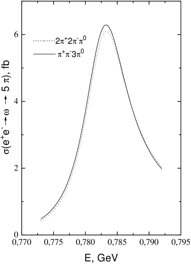
Figure 11: The excitation curve of the decays $\omega\to 5\pi$ in $e^{+}e^{-}$ annihilation.

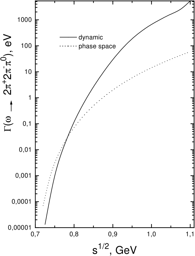
Figure 12: The energy dependence of the $\omega\to 2\pi^{+}2\pi^{-}\pi^{0}$ partial width.

are plotted in Fig. 11. The curves are asymmetric and shifted by 0.7 MeV towards the higher values from the $\omega$ mass because of strong energy dependence of $\Gamma_{\omega\to 5\pi}(s)$, see Fig. 12 below. As is seen, both isotopic channels have approximately equal branching ratios and almost coincident excitation curves in the $\omega$ resonance region. This can be understood as follows. The matrix elements squared numerically are approximately the same in the near-to-threshold region, since the pion mass difference is smeared in the sum of various contributions. Hence, they are cancelled in the ratio of two partial widths, leaving the ratio of the phase space volumes. Using the nonrelativistic expression for the phase space volume of the five pion final state from Ref. byck , one obtains

$${B(\omega\to 2\pi^{+}2\pi^{-}\pi^{0},m^{2}_{\omega})\over B(\omega\to\pi^{+}\pi^{-}3\pi^{0},m^{2}_{\omega})}={3m_{\pi^{+}}\over 2m_{\pi^{0}}}\left({2m_{\pi^{+}}+3m_{\pi^{0}}\over 4m_{\pi^{+}}+m_{\pi^{0}}}\right)^{3/2}\left({m_{\omega}-4m_{\pi^{+}}-m_{\pi^{0}}\over m_{\omega}-2m_{\pi^{+}}-3m_{\pi^{0}}}\right)^{5}=0.93$$ (49)

to be compared to 0.96 calculated from Eq. (47). The ratio of the Bose symmetry factors 3/2 compensates the smaller phase space volume of the final state $2\pi^{+}2\pi^{-}\pi^{0}$ as compared to $\pi^{+}\pi^{-}3\pi^{0}$ one. In the meantime, the energy dependence of the $\omega\to 5\pi$ partial width in the dynamical model is drastically different from that in the model of the Lorentz-invariant phase space (lips). In the latter, one has the following expression for the $\omega\to 5\pi$ partial width:

$$\Gamma_{\omega\to 5\pi}^{(\rm lips)}(s)=\Gamma_{\omega\to 5\pi}(m^{2}_{\omega}){W_{5\pi}(s)\over W_{5\pi}(m^{2}_{\omega})},$$ (50)

where $\Gamma_{\omega\to 5\pi}(m^{2}_{\omega})$ is the partial width evaluated with the dynamical amplitudes given in Sec. II, and the expression for the Lorentz invariant phase space volume is

$$W_{5\pi}(s) = {\pi^{4}\over(2\pi)^{11}32s^{3/2}N_{\rm sym}}\int_{(m_{1}+m_{2}+m_{3}+m_{4})^{2}}^{(\sqrt{s}-m_{5})^{2}}{ds_{1}\over s_{1}}\lambda^{1/2}(s,s_{1},m^{2}_{5})\int_{(m_{1}+m_{2}+m_{3})^{2}}^{(\sqrt{s_{1}}-m_{4})^{2}}{ds_{2}\over s_{2}}\times$$ (51)

$$\lambda^{1/2}(s_{1},s_{2},m^{2}_{4})\int_{(m_{1}+m_{2})^{2}}^{(\sqrt{s_{2}}-m_{3})^{2}}{ds_{3}\over s_{3}}\lambda^{1/2}(s_{2},s_{3},m^{2}_{3})\lambda^{1/2}(s_{3},m^{2}_{1},m^{2}_{2}),$$

with $m_{i}$, $i=1,...5$ being the mass of the meson $\pi_{i}$, and

$$\lambda(x,y,z)=x^{2}+y^{2}+z^{2}-2xy-2xz-2yz.$$ (52)

The predictions of both models for the energy dependence of $\Gamma_{\omega\to 2\pi^{+}2\pi^{-}\pi^{0}}(s)$ are plotted in Fig. 12. The plot for the $\pi^{+}\pi^{-}3\pi^{0}$ final state looks similar and is not given here. The faster growth of the partial width in the dynamical model as compared to the phase space one is due to the resonance enhancement arising from opening of the $\rho$ production in the intermediate state.

Let us relax the constraint Eq. (41) on the parameters $c_{1,2,3}$. To be specific, we choose $-2\leq c_{2}\leq 2$ instead of $c_{2}=0$ assumed earlier. The corresponding ratio $\gamma=(c_{1}+c_{2}-c_{3})/4c_{3}$ parametrizing the strength of the neglected terms then falls into the interval $-1\leq\gamma\leq 1$, or $-1\leq c_{1}/c_{3}\leq 3$. The branching ratios $B_{\omega\to 5\pi}$ evaluated with the new parameters deviate by less than one percent from those evaluated at $\gamma=0$.

IV The evaluation of the $\phi\to\pi^{+}\pi^{-}3\pi^{0}$ and $\phi\to 2\pi^{+}2\pi^{-}\pi^{0}$ branching ratios.

As is known, chiral models, including HLS, do not possess the terms responsible for the decays of $\phi$ meson into final states containing nonstrange quarks only. However, one can guess the general form of such terms guided by both the OZI rule violation in the decay $\phi\to\rho\pi\to\pi^{+}\pi^{-}\pi^{0}$ and by the Adler condition.

There are two feasible models of the OZI-suppressed $\phi\to\rho\pi$ decay amplitude. The first one is the $\phi\omega$ mixing model, where the above decay proceeds due to the small admixture of nonstrange quarks in the flavor wave function of $\phi$ meson composed mostly of the pair of strange quarks. In the second model $\phi$ goes to $\rho\pi$ directly, see Ref. ach95 . Earlier we pointed out that there are no particular reasons to prefer one model to another, and possible ways to resolve the issue were pointed out ach95 ; ach93 . Recent SND data snd03 point to a sizeable coupling constant of direct $\phi\to\rho\pi$ transition, assuming the dependence $|\psi(0,m_{V})|^{2}\propto m^{2}_{V}$ach95 of the wave function of the vector $q\bar{q}$ bound state at the origin on the mass $m_{V}$ of this state. It should be noted that the assumed dependence agrees remarkably good with the ratios of the measured leptonic widths of the vector quarkonia $\rho$, $\omega$, $\phi$, $J/\psi$, and $\Upsilon(1S)$.

The decays $\phi\to 5\pi$ are treated slightly differently in the above models of OZI rule violation. Let us consider them in due turn. In the model of $\phi\omega$ mixing $\phi$ goes to the off-mass-shell $\omega$ which decays as is considered in Sec. II. Hence, one can immediately obtain

$$\Gamma_{\phi\to 5\pi}(m^{2}_{\phi})=|\varepsilon_{\phi\omega}(m^{2}_{\phi})|^{2}\Gamma_{\omega\to 5\pi}(m^{2}_{\phi}),$$ (53)

where $\varepsilon_{\phi\omega}(m_{\phi})$ is the complex parameter of $\phi\omega$ mixing taken at the $\phi$ mass. It can be evaluated as

$$|\varepsilon_{\phi\omega}(m^{2}_{\phi})|^{2}={\Gamma_{\phi\to 3\pi}(m^{2}_{\phi})\over\Gamma_{\omega\to 3\pi}(m^{2}_{\omega})}\cdot r=3.04\times 10^{-3},$$

where $r=3.5\times 10^{-2}$ is the ratio of the three pion phase space volumes at the $\omega$ and $\phi$ peaks.

If $\phi\omega$ mixing is negligible, one should introduce a number of new OZI rule violating parameters to quantify the $\phi\to 5\pi$ decay amplitude. Guided by the condition of chiral symmetry expressed as the demand that the correct decay amplitude should fulfill the Adler condition, it is reasonable to expect that the effective Lagrangian describing anomalous OZI suppressed decays of $\phi$ meson looks similar to the Lagrangian Eq. (9),

$$\cal{L}^{\rm an}_{\phi,\rho,\pi} = {1\over 2f^{3}_{\pi}}(\beta_{1}-\beta_{2}-\beta_{3})\varepsilon_{\mu\nu\lambda\sigma}\phi_{\mu}\left(\partial_{\nu}\bm{\pi}\cdot[\partial_{\lambda}\bm{\pi}\times\partial_{\sigma}\bm{\pi}]\right)+$$ (54)

$${1\over 8f^{5}_{\pi}}\left[-\beta_{1}+{5\over 3}\left(\beta_{2}+\beta_{3}\right)\right]\varepsilon_{\mu\nu\lambda\sigma}\phi_{\mu}\left(\partial_{\nu}\bm{\pi}\cdot[\partial_{\lambda}\bm{\pi}\times\partial_{\sigma}\bm{\pi}]\right)\bm{\pi}^{2}-$$

$${2\beta_{3}g\over f_{\pi}}\varepsilon_{\mu\nu\lambda\sigma}\partial_{\mu}\phi_{\nu}\left\{\left(\bm{\rho}_{\lambda}\cdot\partial_{\sigma}\bm{\pi}\right)+{1\over 6f^{2}_{\pi}}\left[\left(\bm{\rho}_{\lambda}\cdot\bm{\pi}\right)\left(\bm{\pi}\cdot\partial_{\sigma}\bm{\pi}\right)-\bm{\pi}^{2}\left(\bm{\rho}_{\lambda}\cdot\partial_{\sigma}\bm{\pi}\right)\right]\right\}-$$

$${2g\over f_{\pi}}(\beta_{1}+\beta_{2}-\beta_{3})\varepsilon_{\mu\nu\lambda\sigma}\phi_{\mu}\left\{\frac{1}{4f^{2}_{\pi}}\left(\partial_{\nu}\bm{\pi}\cdot\bm{\rho}_{\lambda}\right)\left(\bm{\pi}\cdot\partial_{\sigma}\bm{\pi}\right)-{g\over 4}\left(\left[\bm{\rho}_{\nu}\times\bm{\rho}_{\lambda}\right]\cdot\partial_{\sigma}\bm{\pi}\right)\right\},$$

where $\beta_{1,2,3}$ are the above mentioned parameters responsible for the violation of the OZI rule in the $\phi\to 5\pi$ decays of $\phi$ meson. The analysis similar to that presented in Sec. II.1.1 and II.2.1 shows that the $\phi\to 5\pi$ decay amplitudes obtained from the Lagrangian (54), satisfy the Adler condition. As is evident from Eq. (54), one should identify the coupling constant of direct $\phi\to\rho\pi$ transition as

$$g_{\phi\rho\pi}=-{2\beta_{3}g\over f_{\pi}}=0.8\mbox{ GeV}^{-1},$$ (55)

where the magnitude of $g_{\phi\rho\pi}$ is obtained from the $\phi\to 3\pi$ partial widths, while the positive sign (relative to $g_{\omega\rho\pi}$ usually taken to be positive) is fixed by the $\phi\omega$ interference pattern observed in the energy dependence of the $e^{+}e^{-}\to\pi^{+}\pi^{-}\pi^{0}$ reaction cross section snd01 . Note that we neglect the unitarity corrections to $g_{\phi\rho\pi}$ ach00a , because they are irrelevant in the context of the present work. Next, it seems to be no sizeable point like $\phi\to\pi^{+}\pi^{-}\pi^{0}$ contribution. Indeed, first, the existing upper limit to the branching ratio of the non-$\rho\pi$ intermediate state direct transition $\phi\to\pi^{+}\pi^{-}\pi^{0}$ obtained by SND group at VEPP-2M, is very small snd02 ,

$$B^{\rm direct}(\phi\to\pi^{+}\pi^{-}\pi^{0})<6\times 10^{-4}(\mbox{90 \% C.L.}).$$ (56)

Second, the KLOE Collaboration at DA$\Phi$NE gives the phase space averaged direct $\phi\to\pi^{+}\pi^{-}\pi^{0}$ contribution at the level of 1% kloe of the total $\pi^{+}\pi^{-}\pi^{)}$ decay rate. Hence, in a close analogy with the $\omega$ case, one can set

$$\beta_{1}-\beta_{2}-\beta_{3}=0.$$ (57)

The results of relaxing this conditions are discussed at the end of the present Section. The magnitude $\beta_{3}=-0.006$ is fixed according to Eq. (55) by the $\phi\to 3\pi$ partial widths. After all, the ratio $\beta_{1}/\beta_{3}$ remains arbitrary. We set

$$\beta_{1}+\beta_{2}-\beta_{3}=0,$$ (58)

hence $\beta_{1}=\beta_{3}\mbox{, }\beta_{2}=0$, so that the $\phi\to 5\pi$ decay amplitudes are determined by the only parameter $\beta_{3}$ and looks like Eq. (39) for the $\omega\to 5\pi$ decay, with the replacement $g_{\omega\rho\pi}\to g_{\phi\rho\pi}$. The tensor $T_{\lambda\sigma}$ is the same as in the $\omega\to 5\pi$ decay amplitude. Under these assumptions both mentioned models for the OZI rule violating decay $\phi\to 3\pi$ give similar results for branching ratios of the decays $\phi\to 5\pi$. These are the following:

$$B_{\phi\to\pi^{+}\pi^{-}3\pi^{0}}(m^{2}_{\phi}) = 2.4\times 10^{-7}\mbox{, }B^{\rm aver}_{\phi\to\pi^{+}\pi^{-}3\pi^{0}}=1.8\times 10^{-7},$$

$$B_{\phi\to 2\pi^{+}2\pi^{-}\pi^{0}}(m^{2}_{\phi}) = 6.9\times 10^{-7}\mbox{, }B^{\rm aver}_{\phi\to 2\pi^{+}2\pi^{-}\pi^{0}}=4.9\times 10^{-7},$$ (59)

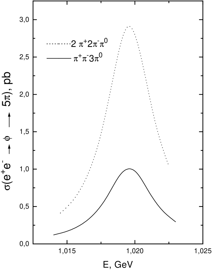
Figure 13: The excitation curve of the decays $\phi\to 5\pi$ in $e^{+}e^{-}$ annihilation.

where $B^{\rm aver}$, useful for the reactions of peripheral production, stands for the branching ratio averaged over $\pm\Gamma_{\phi}$ region around $\phi$ peak [use Eq. (46) with replacement $\omega\to\phi$]. The evaluation of the excitation curve of the decays $\phi\to 5\pi$ in $e^{+}e^{-}$ annihilation performed according to Eq. (48) (with the replacement $\omega\to\phi$) is plotted in Fig. 13. Notice that the ratio of the branching ratios of two isotopic modes at $\phi$ peak is

$${B_{\phi\to 2\pi^{+}2\pi^{-}\pi^{0}}(m^{2}_{\phi})\over B_{\phi\to\pi^{+}\pi^{-}3\pi^{0}}(m^{2}_{\phi})}=2.9,$$ (60)

to be compared to the figure of 1.3 obtained from the simple evaluation of the ratio of nonrelativistic phase space, see Eq. (49) with the replacement $m_{\omega}\to m_{\phi}$. In the present case, the difference with the exact evaluation is sizeable, because now the phase space model is inadequate due to the strong $\rho$ and $\omega$ ($\rho\to\omega\pi\to 4\pi$) resonance production in the intermediate states. The $\phi\to 5\pi$ excitation curve is plotted in Fig. 13.

In this respect, it is interesting to look at the dynamical behavior of the specific contributions to the $\phi\to 5\pi$ decay amplitudes in another way. Let us evaluate, for this purpose, the contribution to $B_{\phi\to\pi^{+}\pi^{-}3\pi^{0}}$ of the diagrams Fig. 1, at the $\phi$ mass. (Notice that now $\omega$ in initial state should be replaced with $\phi$ in all the diagrams, and the effective $g_{\phi\rho\pi}$ is understood at the corresponding expression, while other couplings are related with it as is explained earlier in this Section). The $\rho$ meson in these diagrams is resonant. Indeed, choosing the averaged pion energy from the condition of equilibrium as $\langle E_{\pi}\rangle=m_{\phi}/5$, one finds that the invariant mass of four pions emitted in the transition $\rho\to 4\pi$ is $m_{4\pi}\simeq m_{\rho}$. The evaluation gives $B^{\rm resonant}_{\phi\to\pi^{+}\pi^{-}3\pi^{0}}=2.1\times 10^{-7}$. All the remaining contributions with the non-resonant intermediate $\rho$ meson, see Fig. 2-4, amount to $B^{\rm non-resonant}_{\phi\to\pi^{+}\pi^{-}3\pi^{0}}=0.34\times 10^{-7}$, which constitutes $16\%$ of the resonant contribution. Notice that the seemingly resonant diagrams Fig. 2 and 7 do not, in fact, possess this property, because three pions produced from the transition $\pi\to 3\pi$, push $\rho$ meson away from the resonance. Indeed, the invariant mass of the pion pair in the transition $\rho\to 2\pi$ evaluated assuming the same average pion energy as above, falls into the interval $2m_{\pi}\leq m_{2\pi}\leq 0.41$ GeV, which is far from the resonance value. The phase space averaged relative phase between the resonant and non-resonant contributions calculated with the help of given branching ratios and that given in Eq. (59) is about $\delta=91^{\circ}$. Correspondingly, similar calculations for another isotopic state $2\pi^{+}2\pi^{-}\pi^{0}$ state give $B^{\rm resonant}_{\phi\to 2\pi^{+}2\pi^{-}\pi^{0}}=6.2\times 10^{-7}$ from Fig. 6, $B^{\rm non-resonant}_{\phi\to 2\pi^{+}2\pi^{-}\pi^{0}}=0.70\times 10^{-7}$ from Fig. 7-9, and $\delta=89^{\circ}$. In the present case, the non-resonant contribution constitutes about $11\%$ of the resonant one. The above estimates illustrate clearly the dominance of the diagrams with the resonant $\rho$ meson in the intermediate state in the decay $\phi\to 5\pi$, because the resonant and the smaller non-resonant contributions add incoherently in the case of the $\phi\to 5\pi$ decay. For comparison, opposite situation takes place in the case of the $\omega\to 5\pi$ decay amplitudes, see the corresponding calculations in Sec. III, where the smaller non-resonant contribution to the decay amplitude adds almost in phase with the resonant one and by this reason is essential.

The relaxing the constraint Eq. (58) to $-1\leq(\beta_{1}+\beta_{2}-\beta_{3})/4\beta_{3}\leq 1$ analogous to that discussed in the $\omega$ case implies even smaller deviations of $B_{\phi\to 5\pi}$ in comparison with the $\omega$ case, because the terms in the amplitude which are sensitive to the parameter in the above inequality, are almost incoherent with the dominant ones. On the other hand, relaxing the constraint of the absence of the point like $\phi\to\pi^{+}\pi^{-}\pi^{0}$ amplitude, see Eq. (57), gives the following. Using the KLOE data Ref. kloe , one can estimate the combination characterizing the pointlike $\phi\to\pi^{+}\pi^{-}\pi^{0}$ vertex as $|3(\beta_{1}-\beta_{2}-\beta_{3})/2\beta_{3}m^{2}_{\rho}|\simeq 1$. The evaluation of $B_{\phi\to 5\pi}$, keeping the constraint Eq. (58), gives the results deviating by $\pm 8\%$ (depending on the sign of the above combination) from those obtained under the constraint Eq. (57).

All the above discussion shows that the branching ratios of the decays $\phi\to\pi^{+}\pi^{-}3\pi^{0}$ and $\phi\to 2\pi^{+}2\pi^{-}\pi^{0}$ are determined within the conservatively estimated accuracy 20% by the well studied OZI rule violating transition of $\phi$ meson to the $\rho\pi$ state followed by the transition $\rho\to 4\pi$ in the model independent way.

V Discussion and conclusion.

In view of the fact that there are three (or even four, if one includes radiative decays, see Ref. hls1 ; hls2 ) independent constants in the effective chiral Lagrangian describing anomalous decays of $\omega$ (and $\phi$) mesons, one can only consider some scenarios of what may happen. We restrict ourselves by considering only the strong decays. In principle, the study of the Dalitz plot in the $\omega\to\pi^{+}\pi^{-}\pi^{-}$ decay allows to extract $c_{3}$ and $(c_{1}-c_{2})/c_{3}$ by isolating the $\rho$ pole and non-$\rho$ pole contributions, because the density on this plot is proportional, omitting the $\omega\rho$ interference term in the $\pi^{+}\pi^{-}$ mass spectrum, to the factor

$${d^{2}N\over dm_{+}dm_{-}}\propto\left|{1\over D_{\rho}(q_{1}+q_{2})}+{1\over D_{\rho}(q_{1}+q_{3})}+{1\over D_{\rho}(q_{2}+q_{3})}+3{c_{1}-c_{2}-c_{3}\over 2c_{3}m^{2}_{\rho}}\right|^{2},$$ (61)

where $m_{+}^{2}=(q_{1}+q_{3})^{2}$, $m_{-}^{2}=(q_{2}+q_{3})^{2}$. Notice in this respect that the combination of parameters of the low energy effective Lagrangian entering in the non-$\rho$-pole term in Eq. (61) should be treated the low energy limit of all possible contributions from the transitions $\omega\to\rho^{\prime}\pi$, $\rho^{\prime\prime}\pi$ etc. If one assumes the direct transitions are responsible for the decays of $\phi$ meson to the states containing no strange quarks, the same will be true for the parameters $\beta_{1,2,3}$ characterizing the OZI rule violating decays $\phi\to 3\pi$ and $\phi\to 5\pi$. In the model of $\phi\omega$ mixing, the $\phi\to 5\pi$ decay amplitude contain no additional free parameters as compared to the case of the $\omega\to 5\pi$ decay. It should be recalled that both models can be, in principle, discriminated by the careful study of the $\phi\omega$ interference minimum in the energy dependence of the $e^{+}e^{-}\to\pi^{+}\pi^{-}\pi^{0}$ reaction cross section or by the ratio of the leptonic widths of $\omega$ and $\phi$ mesons ach95 ; ach93 ; snd03 . On the other hand, within the accuracy of 20%, the branching ratios of the $\phi\to 5\pi$ decays can be evaluated in a model independent way, see the discussion at the end of Sec. IV.

The excitation curves of the decays $\omega\to 5\pi$ and $\phi\to 5\pi$ in $e^{+}e^{-}$ annihilation can be used to evaluate the expected number of these decays at $\omega$ and $\phi$ peaks. With the luminosity $L=10^{32}$ cm^-2 s^-1 at $\omega$ peak, one may hope to observe three events of the decays $\omega\to\pi^{+}\pi^{-}3\pi^{0}$ and $2\pi^{+}2\pi^{-}\pi^{0}$ per each mode bimonthly. With the same luminosity at the $\phi$ peak, the observation of, respectively, 750 (250) $\phi\to 2\pi^{+}2\pi^{-}\pi^{0}$ ($\phi\to\pi^{+}\pi^{-}3\pi^{0}$) decays per month is feasible. Note that the existing upper limit is $B_{\phi\to 2\pi^{+}2\pi^{-}\pi^{0}}<4.6\times 10^{-6}$ ($90\%$ C.L.) cmd200 . With the luminosity $L=500\mbox{ pb}^{-1}$ already attained at $\phi$ factory DA$\Phi$NE kloe1 , one could gain about 1685 events of the decay $\phi\to 5\pi$ proceeding via chiral mechanisms considered in the present paper. The possible non-chiral-model background from the dominant decay $\phi\to K_{L}K_{S}$, $K_{L}\to 3\pi$, $K_{S}\to 2\pi$ is well cut from the considered chiral mechanism by macroscopic distances kaons fly away. Rare decay $\phi\to\eta\pi^{+}\pi^{-}$ whose branching ratio was estimated ach84 ; ach92 at the level $B_{\phi\to\eta\pi^{+}\pi^{-}}\sim 3\times 10^{-7}$, is cut by removing events in the vicinity of the $\eta$ peak in the three pion distribution observed in the five pion events cmd200 .

In the present work, we neglect the contribution of the $a_{1}(1260)$ meson. This is justifiable because both the $\omega(782)$ and $\phi(1020)$ peaks are deep under the threshold of $a_{1}\pi$ production. As is known, the approach to chiral dynamics based on HLS, allows to take the axial vector mesons into account hls1 ; hls2 . This is the theme of future work.

*

Appendix A Relations expressing Lorentz scalar products through the Kumar variables

In this Appendix, the relations expressing the Lorentz scalar products $(q_{i},q_{j})$ through Lorentz-invariant variables are presented. Given the pion momentum assignment according to

$$\omega_{q}\to\pi_{q_{1}}\pi_{q_{2}}\pi_{q_{3}}\pi_{q_{4}}\pi_{q_{5}},$$ (62)

the eight Kumar variables kumar are defined as

$$s_{1} = (q-q_{1})^{2},$$

$$s_{2} = (q-q_{1}-q_{2})^{2},$$

$$s_{3} = (q-q_{1}-q_{2}-q_{3})^{2},$$

$$u_{1} = (q-q_{2})^{2},$$

$$u_{2} = (q-q_{3})^{2},$$

$$u_{3} = (q-q_{4})^{2}$$

$$t_{2} = (q-q_{2}-q_{3})^{2},$$

$$t_{3} = (q-q_{2}-q_{3}-q_{4})^{2}.$$ (63)

Associated with them, but not independent, are the following:

$$s^{\prime}_{2} = (q_{1}+q_{2})^{2},$$

$$s^{\prime}_{3} = (q_{1}+q_{2}+q_{3})^{2},$$

$$s^{\prime}_{4} = (q-q_{5})^{2},$$

$$t^{\prime}_{2} = (q_{2}+q_{3})^{2},$$

$$t^{\prime}_{3} = (q_{2}+q_{3}+q_{4})^{2}.$$ (64)

Then the greater part of the Lorentz scalar products of the pion momenta can be expressed through the variables Eq. (63) and (64):

$$(q_{1},q_{2}) = {1\over 2}(s^{\prime}_{2}-m^{2}_{1}-m^{2}_{2}),$$

$$(q_{1},q_{3}) = {1\over 2}(s^{\prime}_{3}-s^{\prime}_{2}-t^{\prime}_{2}+m^{2}_{2}),$$

$$(q_{1},q_{4}) = {1\over 2}(t_{2}-t_{3}-s_{3}+m^{2}_{5}),$$

$$(q_{1},q_{5}) = {1\over 2}(t_{3}-m^{2}_{1}-m^{2}_{5}),$$

$$(q_{2},q_{3}) = {1\over 2}(t^{\prime}_{2}-m^{2}_{2}-m^{2}_{3}),$$

$$(q_{4},q_{5}) = {1\over 2}(s_{3}-m^{2}_{4}-m^{2}_{5}).$$ (65)

The remaining scalar products

$$(q_{3},q_{5}) = {1\over 2}(s_{2}-s_{3}-m^{2}_{3})-(q_{3},q_{4}),$$

$$(q_{2},q_{4}) = {1\over 2}(t^{\prime}_{3}-t^{\prime}_{2}-m^{2}_{4})-(q_{3},q_{4})$$ (66)

can be expressed through $(q_{3},q_{4})$. The latter, using the method of invariant integration outlined in Appendix D of Ref. kumar , can be found as

$$(q_{3},q_{4})={1\over 2}\left[\alpha(s-u_{2}+m^{2}_{3})+\beta(u_{1}-t_{2}-m^{2}_{3})+\gamma(s_{2}-s_{3}-m^{2}_{3})\right],$$ (67)

where

$$\alpha = {1\over\Delta_{M}}(Ft_{2}s_{3}+BCG+ACH-t_{2}BH-C^{2}F-As_{3}G),$$

$$\beta = {1\over\Delta_{M}}(ss_{3}G+ABH+BCF-B^{2}G-sCH-As_{3}F),$$

$$\gamma = {1\over\Delta_{M}}(st_{2}H+ABG+ACF-t_{2}BF-sCG-A^{2}H),$$ (68)

and

$$A = {1\over 2}(s+t_{2}-t^{\prime}_{2}),$$

$$B = {1\over 2}(s+s_{3}-s^{\prime}_{3}),$$

$$C = {1\over 2}(s_{3}+t_{2}-m^{2}_{1}),$$

$$F = {1\over 2}(s-u_{3}+m^{2}_{4}),$$

$$G = {1\over 2}(t_{2}-t_{3}+m^{2}_{4}),$$

$$H = {1\over 2}(s_{3}+m^{2}_{4}-m^{2}_{5}),$$

$$\Delta_{M} = st_{2}s_{3}+2ABC-B^{2}t_{2}-C^{2}s-A^{2}s_{3}.$$ (69)

In the above formulas, $m_{i}$, $i=1,...5$, are the masses of final pions.

References

-
(1)
M. Bando, T. Kugo, S. Uehara et al., Phys.Rev.Lett. 54,
1215 (1985);
M. Bando, T. Kugo, K. Yamawaki, Nucl. Phys. B259, 493 (1985); Progr.Theor.Phys. 73, 1541 (1985); Phys.Rep. 164, 217 (1988). - (2) M. Harada and K. Yamawaki, Phys.Rept.381, 1 (2003), hep-ph/0302103.
- (3) Ö. Kaymakcalan, S. Rajeev, and J. Schechter, Phys.Rev. D30, 594 (1984).
-
(4)
K. Kawarabayashi, M. Suzuki, Phys.Rev.Lett. 16, 255 (1966);
Riazzuddin, Fayyazuddin, Phys.Rev. 147, 1071 (1966). - (5) J. Wess, B. B. Zumino, Phys.Lett. 37B, 95 (1971).
- (6) K. Hagiwara et al., Phys.Rev. D66, 010001 (2002).
- (7) N. N. Achasov and A. A. Kozhevnikov, Phys.Rev. D62, 056011 (2000); JETP 91, 433 (2000); Zh.Eksp.Teor.Fiz. 91, 499 (2000).
- (8) S. Weinberg, Phys.Rev. 166, 1568 (1968).
- (9) R. Kumar, Phys.Rev. 185, 1865 (1969).
- (10) T. W. Sag and G. Szekeres, Math.Comput. 18, 245 (1964).
- (11) E. Byckling and K. Kajantie, Particle Kinematics (Wiley, London, 1973).
- (12) N. N. Achasov and A. A. Kozhevnikov, Phys.Rev. D52, 3119 (1995); Phys.Atom.Nucl. 59, 144 (1996); Yad.Fiz. 59, 153 (1996).
- (13) N. N. Achasov and A. A. Kozhevnikov, Sov.J.Nucl.Phys. 55, 1726 (1992); Yad.Fiz. 55, 3086 (1992). Part.World 3, 125 (1993).
- (14) M. N. Achasov et al., ”Study of the process in the energy region below 0.98 GeV”, hep-ex/0305049. To appear in Phys.Rev.D.
- (15) M. N. Achasov et al., Phys.Rev. D63, 072002 (2001).
- (16) N. N. Achasov and A. A. Kozhevnikov, Phys.Rev. D61, 054005 (2000); Phys.Atom.Nucl. 63, 1936 (2000); Yad.Fiz. 63, 2029 (2000).
- (17) M. N. Achasov et al., Phys.Rev. D65, 032002 (2002).
- (18) A. Aloisio et al., KLOE Collaboration, Phys.Lett. B561, 55 (2003).
- (19) R. R. Akhmetshin et al., Phys.Lett. B491, 81 (2000).
- (20) N. N. Achasov and V. A. Karnakov, JETP Lett. 39, 342 (1984).
- (21) N. N. Achasov and A. A. Kozhevnikov, Int.Journ.Mod.Phys. A7, 4825 (1992); Sov.J.Nucl.Phys. 55, 449 (1992); Yad.Fiz. 55, 809 (1992).
- (22) The KLOE Collaboration, ”Recent results from the KLOE experiment at DANE”, hep-ex/0305108.