Lepton flavour violation in $\bm{e^{\pm}e^{-}\to\ell^{\pm}e^{-}}$ ($\bm{\ell=\mu,\tau}$) induced by R-conserving supersymmetry

Abstract

The lepton flavour violating signals $e^{+}e^{-}\to\ell^{+}e^{-}$ and $e^{-}e^{-}\to\ell^{-}e^{-}\;(\ell=\mu,\tau)$ are studied in the context of low energy R-parity conserving supersymmetry at center of mass energies of interest for the next generation of linear colliders. Loop level amplitudes receive contributions from electroweak penguin and box diagrams involving sleptons and gauginos. Lepton flavour violation is due to off diagonal elements in $SU(2)_{L}$ doublet slepton mass matrix. These masses are treated as model independent free phenomenological parameters in order to discover regions in parameter space where the signal cross section may be observable. The results are compared with (a) the experimental bounds from the non-observation of rare radiative lepton decays $\mu,\tau\to e\gamma$ and (b) the general mSUGRA theoretical scenario with seesaw mechanism where off diagonal slepton matrix entries are generated by renormalization group evolution of neutrino Yukawa couplings induced by the presence of new energy scales set by the heavy $SU(2)_{L}$ singlet neutrino masses. It is found that in $e^{-}e^{-}$ collisions the ($e\tau$) signal can be observable with a total integrated luminosity of 100 fb^-1 and the that the background can be easily suppressed. In $e^{+}e^{-}$ collisions the cross section is smaller and higher luminosities are needed. The experimental bound on the decay $\mu\to e\gamma$ prevents the ($e\mu$) signal from being observable.

I Introduction

In the advent of growing evidence for neutrino oscillations and hence flavour mixing in the lepton sector of the Standard Model (SM), the topic of lepton flavour violation (LFV) has received considerable attention. Non-vanishing neutrino masses in principle induce LFV processes such as $\ell\rightarrow\ell^{\prime}\gamma$. If neutrinos have masses in the eV or sub-eV range, the neutrino generated branching ratio to the latter process is of order ${\cal O}$(10^-40) and therefore unobservably small. On the other hand, in supersymmetric (SUSY) extensions of the SM the soft SUSY breaking potential $V_{soft}$ contains, in general, nondiagonal entries in generation space and therefore additional potential sources for LFV. Even in minimal supergravity scenarios characterized by universal soft mass term for scalar slepton and squark fields, renormalization induces potentially sizable weak scale flavour mixing Gabbiani in $V_{soft}$.

Many experimental efforts have been devoted to search for LFV and lepton number violating reactions, both in rare decays and in high energy accelerators. The strongest bounds on LFV come from the non-observation of radiative lepton decays mega ; cleo1 ; cleo2 :

$$Br(\mu\to e\gamma)<1.2\times 10^{-11},$$ (1)

$$Br(\tau\to e\gamma)<2.7\times 10^{-6},$$ (2)

$$Br(\tau\to\mu\gamma)<1.1\times 10^{-6}.$$ (3)

The four LEP experiments searched for $Z\to\ell^{+}_{i}\ell^{-}_{j},\;\ell=e,\mu,\tau,\;i\neq j$ at the Z peak providing the following upper bounds on branching ratios pdg : $Br(Z\to e\mu)<1.7\times 10^{-6}$, $Br(Z\to e\tau)<9.8\times 10^{-6}$, $Br(Z\to\tau\mu)<1.2\times 10^{-5}$. The high luminosity GigaZ option of the Tesla project desy is expected to probe the above branching ratios down to $\sim{\cal O}(10^{-8},10^{-9})$. A recent study of LFV induced by R-parity conserving SUSY at the Z peak is given in Ref. illa .

However it is interesting to know if such signals can be observed at higher energies. The OPAL collaboration searched for LFV reactions up to the highest center of mass energy reached by LEPII, $\sqrt{s}=209$ GeV opal . One $e^{+}e^{-}\to e\mu$ event was found at $\sqrt{s}=189$ GeV matching all tagging conditions, but it was interpreted as due to initial state radiation opal . This negative result implies the following upper limits (at $95\%$ confidence level) on the cross sections of LFV processes (for $200\;\mbox{GeV}\leq\sqrt{s}\leq 209\;\mbox{GeV}$):

$$\sigma(e^{+}e^{-}\to e\mu)<22\;\mbox{fb},$$ (4)

$$\sigma(e^{+}e^{-}\to e\tau)<78\;\mbox{fb},$$ (5)

$$\sigma(e^{+}e^{-}\to\mu\tau)<64\;\mbox{fb}.$$ (6)

For limits corresponding to lower energies see Ref. opal .

In the following this approach will be pursued further and a detailed study of the reactions

$$e^{+}e^{-} \to \ell^{+}e^{-}\ ,$$

$$e^{-}e^{-} \to \ell^{-}e^{-}\ (\ell=\mu,\tau)$$ (7)

will be presented in the context of SUSY extension of the SM with conserved R-parity for center of mass energies of interest for the next linear collider projects (LC). The processes in Eq. (I) have the advantage of providing a clean final state being easy to identify experimentally (two back to back different flavor leptons), though one has to pay the price of dealing with cross sections of order ${\cal O}(\alpha^{4})$. Previous studies on SUSY induced LFV at a LC (see e.g. lfvee ) were limited to tree level processes for SUSY partner production decaying into final states characterized by very complicated topologies such as $\ell_{i}\ell_{j}+4\,jets+E/$ involving jets and missing energy. A detailed study of cuts and background is necessary to isolate the signal.

The relevant Feynmann diagrams describing the processes in Eq. (I) are shown in Figs. 1, 2, 3. They are the high energy analogue of the box and penguin diagrams that mediate LFV rare decays as e.g. $\mu\to e+\gamma$ or $\mu\to 3e$. Due to the experimental limits on the cross sections and the loop nature of the process event rates are expected - even in more optimistic cases - to be relatively small. However, when the energy dependence of four-point and three-point functions is taken into account the amplitudes can show a resonance behavior as the energy approaches thresholds for particle production. This is a consequence of the discontinuity of the derivative of the real part of a loop amplitude where it develops an imaginary part (Cutkosky rule). The cross section in this point may increase by orders of magnitude. We have shown in a recent paper Cannoni on LFV induced by heavy Majorana neutrinos that the enhancement may be quite dramatic in some regions of the parameter space.

The plan of the paper is the following. Sec. II discusses LFV in R-parity conserving SUSY and gives an outline of the calculation. Sec. III contains numerical results for the signal cross section and a discussion of possible backgrounds. Sec. IV is devoted to a comparison with bounds from rare LFV lepton decays. Sec. V contains the conclusions. Appendices A and B give details of the lagrangians and numerical tools used in the calculation. Finally, in Appendix C helicity amplitudes for $e^{+}e^{-}$ and $e^{-}e^{-}$ collisions are given.

II SUSY origin of lepton flavour violation

One of the most important challenges in contemporary particle physics is to understand the origin of neutrino masses. Quite generally this requires new fields to be added to those of the SM and/or those of its minimal SUSY version (MSSM). In the seesaw framework - the simplest scenario for the explanation of neutrino masses - and its SUSY extension, the superpotential contains three $SU(2)_{L}$ singlet neutrino superfields $N_{i}$ with the following couplings borma ; hisa1 ; hisa2 ; casas ; hisa3 :

$$W=(Y_{\nu})_{ij}\varepsilon_{\alpha\beta}H_{2}^{\alpha}N_{i}L^{\beta}_{j}+\frac{1}{2}(M_{R})_{i}N_{i}N_{i}.$$ (8)

Here $H_{2}$ is a Higgs doublet superfield, $L_{i}$ are the $SU(2)_{L}$ doublet lepton superfields, $Y_{\nu}$ is a Yukawa coupling matrix and $M_{R}$ is the $SU(2)_{L}$ singlet neutrino mass matrix. As is usually done the basis has been chosen such that $M_{R}$ is diagonal. The effective low energy neutrino mass matrix is given by

$${\cal M}_{\nu}=m_{D}^{T}M_{R}^{-1}m_{D},$$ (9)

where $m_{D}=v_{2}(Y_{\nu})_{ij}/{\sqrt{2}}$ is the Dirac neutrino mass matrix and $v_{2}=\langle H_{2}^{0}\rangle$.

Standard mSUGRA models contain an universal GUT scale (i.e. at the energy scale where the coupling constants unify) scalar field mass term $m_{0}$. At low energies the renormalization group equations (RGE) produce diagonal slepton mass matrices. With the additional Yukawa couplings in Eq. (8) and a new mass scale ($M_{R}$) the RGE evolution of the parameters is modified: assuming that $M_{R}$ is the mass scale of heavy right-handed neutrinos, the RGE from GUT scale to $M_{R}$ induce off-diagonal matrix elements in $(m^{2}_{\tilde{L}})_{ij}$. In the one loop approximation the off-diagonal elements are casas :

$$(m^{2}_{\tilde{L}})_{ij}\simeq-\frac{1}{8\pi^{2}}(3+a^{2}_{0})m_{0}^{2}(Y_{\nu}^{\dagger}Y_{\nu})_{ij}\ln\left(\frac{M_{GUT}}{M_{R}}\right).$$ (10)

Here $a_{0}$ is a dimensionless parameter appearing in the matrix of trilinear mass terms $A_{\ell}=Y_{\ell}a_{0}m_{0}$ contained in $V_{soft}$.

The slepton mass eigenstates are obtained diagonalizing the slepton mass matrices. The corresponding mixing matrices induce LFV couplings in the lepton-slepton-gaugino vertices $\tilde{\ell}^{\dagger}_{L_{i}}{U_{L}}_{ij}\tilde{\ell}_{L_{j}}\chi$. The same effect on the mass matrix of $SU(2)_{L}$ singlet charged sleptons $(m^{2}_{\tilde{R}})_{ij}$ is smaller casas ; hisa3 .

The magnitude of LFV effects will depend on the RGE induced non diagonal entries and ultimately on the neutrino Yukawa couplings $(Y_{\nu})_{ij}$. These in turn depend on the fundamental theory in which this mechanism is embedded (for example $SU(5)$ or $SO(10)$ SUSY GUT hisa3 ; biqi ; masiso10 ) and on the particular choice of texture for the neutrino mass matrix casas ; ellis ; pas . The rate of LFV transitions like $\ell_{i}\to\ell_{j}$, $i\neq j$, $\ell=e,\mu,\tau$ induced by the lepton-slepton-gaugino vertex is determined by the mixing matrix ${U_{L}}_{ij}$ that, as stated above, is model dependent. In a model independent way, however, one can take the lepton, slepton, gaugino vertex flavour conserving with the slepton in gauge eigenstates, so that LFV is given by mass insertion of non diagonal slepton propagators Gabbiani ; illa ; hisa1 .

In a similar spirit, the phenomenological study presented in this paper will be quite model independent and in order to keep the discussion simple the mixing of only two generations is considered, so that the slepton and sneutrino mass matrix is:

$$\tilde{m}^{2}_{{L}}=\left(\begin{array}[]{cc}\tilde{m}^{2}&\Delta m^{2}\\ \Delta m^{2}&\tilde{m}^{2}\end{array}\right),$$ (13)

with eigenvalues: $\tilde{m}^{2}_{\pm}=\tilde{m}^{2}\pm\Delta m^{2}$ and maximal mixing matrix

$$U=\frac{1}{\sqrt{2}}\left(\begin{array}[]{cc}1&1\\ 1&-1\end{array}\right).$$ (16)

Under these assumptions the LFV propagator in momentum space for a scalar line is

$$\langle\tilde{\ell}_{i}\tilde{\ell}^{\dagger}_{j}\rangle_{0} = \frac{i}{2}\left(\frac{1}{p^{2}-\tilde{m}^{2}_{+}}-\frac{1}{p^{2}-\tilde{m}^{2}_{-}}\right)$$ (17)

$$= i\frac{\Delta m^{2}}{(p^{2}-\tilde{m}^{2}_{+})(p^{2}-\tilde{m}^{2}_{-})}\ ,$$ (18)

while a lepton flavour conserving (LFC) scalar line is described by

$$\langle\tilde{\ell}_{i}\tilde{\ell}^{\dagger}_{i}\rangle_{0}=\frac{i}{2}\left(\frac{1}{p^{2}-\tilde{m}^{2}_{+}}+\frac{1}{p^{2}-\tilde{m}^{2}_{-}}\right).$$ (19)

Therefore the essential parameter that controls the LFV signal is

$$\delta_{LL}=\frac{\Delta m^{2}}{\tilde{m}^{2}}.$$ (20)

Before presenting detailed calculations a qualititave order of magnitude estimate of the cross section can be given using dimensional arguments. Consider for simplicity a box diagram. Neglecting the external momenta in the loop propagators and indicating with $m_{S}$ a typical SUSY mass, one has for the amplitude in the case of a scalar four point function:

$${\cal M}\simeq\frac{g^{4}}{(4\pi)^{2}}\,s\,m_{S}^{2}\,\frac{m_{S}^{2}{\Delta m^{2}}}{m_{S}^{8}}.$$ (21)

The constant comes from couplings and loop integration, the factor $s$ from the spinorial part, the mass squared factor from the numerator of the two gaugino propagators and the last factor from the loop integral. The corresponding total cross section (assuming polarized initial particles) is:

$$\sigma\simeq\frac{1}{16\pi}\left(\frac{\alpha}{\sin^{2}\theta_{W}}\right)^{4}\delta^{2}_{LL}\frac{s}{m^{4}_{S}}.$$ (22)

Taking $m_{S}=100$ GeV, $\delta_{LL}=0.1$ and $\sqrt{s}=200$ GeV one has $\sigma\simeq 1.3\times 10^{-2}$ fb while with $\sqrt{s}=500$ GeV $\sigma\simeq 8$ fb. With an annual integrated luminosity of order $L_{0}$=100 fb^-1 one may expect an observable signal.

However this estimate is clearly too crude: it gives a linear increase with $s$ while one expects at high energies, $\sqrt{s}>>m_{S}$, a cross section which scales as $s^{-1}$. To get a realistic result it is necessary to compute exactly the energy dependence of the loop integrals and the interference among all contributing graphs.

III Numerical results

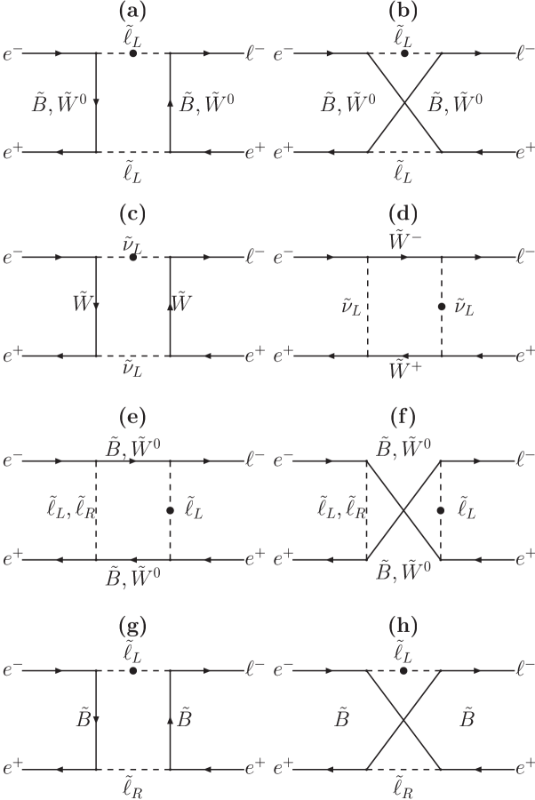
Figure 1: Box diagrams for $e^{+}e^{-}$ collisions. The full black dot in a scalar line denotes the lepton flavour violating propagator (Eq. 18).

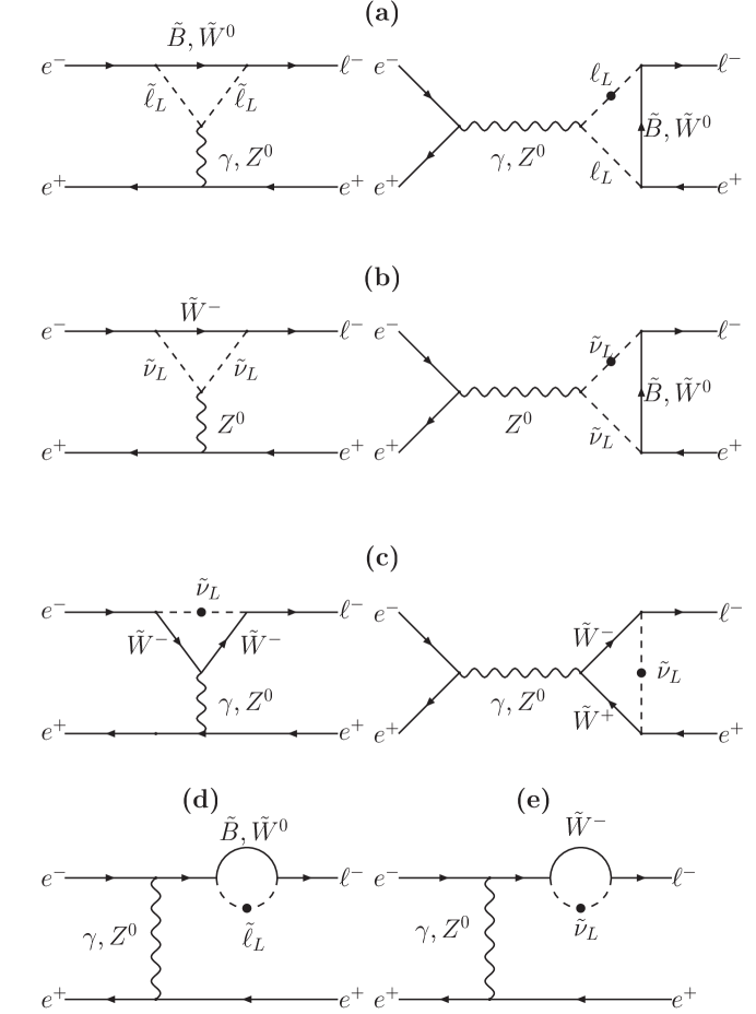
Figure 2: Penguin and external legs diagrams for $e^{+}e^{-}$ collisions. The full black dot in a scalar line denotes the lepton flavour violating propagator. In the diagrams where it is not marked it can occour in both lines. Diagrams like (d) and (e) with the gauge boson in the $s$ channel are also present but not shown.

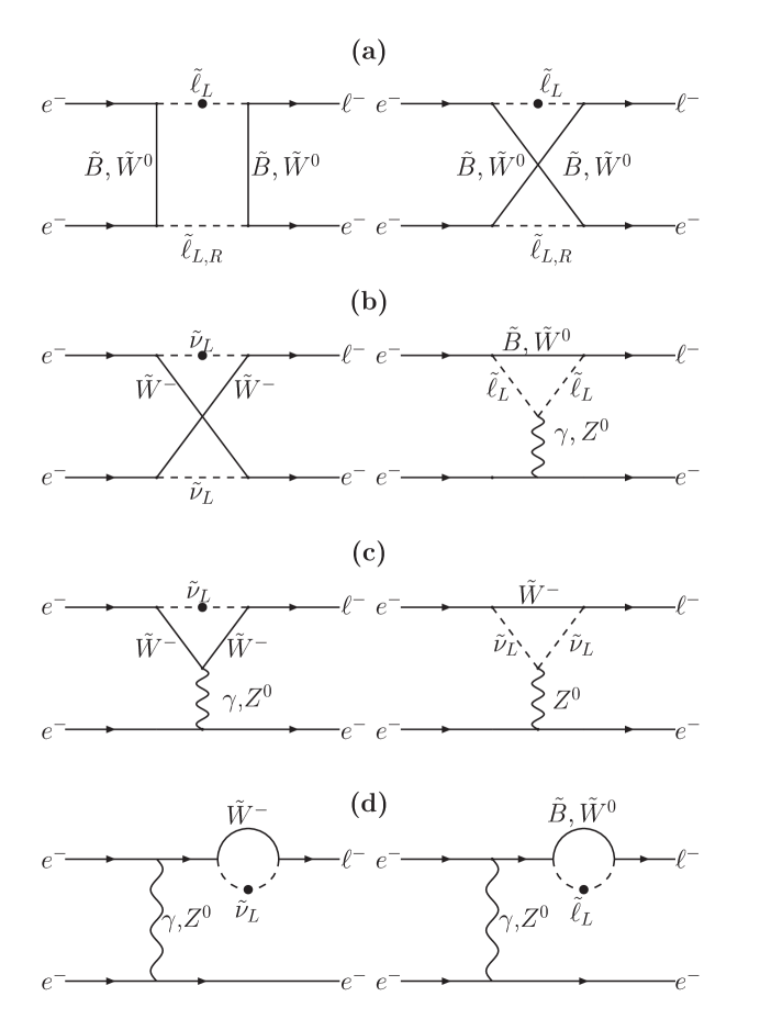
Figure 3: Feynman diagrams for $e^{-}e^{-}$ collisions. The full black dot in a scalar line denotes again the lepton flavour violating propagator. Exchange diagrams are not shown.

In the reactions considered here there are only leptons in the initial and final state. At the energies of a LC lepton masses can be safely neglected and thus all the calculations are done assuming massless external fermions. The signal is suppressed if neutralinos and charginos $\chi^{0,\pm}$ are Higgsino-like, since their coupling is proportional to the lepton masses. For the same reason left-right mixing in the slepton matrix is neglected. Therefore it is assumed that the two lightest neutralinos are pure Bino and pure Wino with masses $M_{1}$ and $M_{2}$ respectively, while charginos are pure charged Winos with mass $M_{2}$, $M_{1}$ and $M_{2}$ being the gaugino masses in the soft breaking potential. The relevant parts of the interaction lagrangian are listed in Appendix A.

Due to the chiral nature of the couplings it is convenient to calculate the amplitudes using the helicity base for spinors: the amplitudes are written in terms of spinor products and a numerical code can be easly implemented to compute both real and imaginary parts. Interference terms are also accounted for by summing the various contributions before taking the absolute modulus squared of the amplitude. In the helicity basis and in the limit of massless fermions there are only two independent spinors, $u_{+}(p)\equiv u_{R}(p)$ and $u_{-}(p)\equiv u_{L}(p)$ with only two non-zero spinor products: $\overline{u}_{R}(p_{a})u_{L}(p_{b})\equiv S(p_{a},p_{b})$, $\overline{u}_{L}(p_{a})u_{R}(p_{b})\equiv T(p_{a},p_{b})$ given by compact expressions, see Appendix B.1. The loop integrals are decomposed in form factors and calculated numerically using the package LoopTools  looptools . The decomposition of loop integrals is obtained for massless external particles and with the loop momenta assigned as described in Fig. 12 of Appendix B.2. The exact dependence from the masses of the particles exchanged in the loop is also given in Appendix B.2. Assigning the momenta in a different way corresponds to a shift of the integration variables and produces different combinations of the loop form factors appearing in the amplitudes. The numerical values remain unchanged.

Besides computational advantages the helicity method clarifies the physics of the processes. The momenta of the external particles are specified as in Eq. (49) (Appendix B) and Fig. 12 (Appendix C), and the following reactions are considered:

$$e^{+}(p_{1},\lambda_{1})e^{-}(p_{2},\lambda_{2}) \to \ell^{-}(p_{3},\lambda_{3})e^{+}(p_{4},\lambda_{4}),$$ (23)

$$e^{-}(p_{1},\lambda_{1})e^{-}(p_{2},\lambda_{2}) \to \ell^{-}(p_{3},\lambda_{3})e^{-}(p_{4},\lambda_{4}).$$ (24)

Here $\lambda_{i}$ denotes the helicity of particle $i$. The corresponding helicity amplitudes ${\cal M}_{j}$ expressed in terms of spinor products and LoopTools form factors are obtained after tedious but straightforward algebra. They can be found in Appendix C.

The integrated cross sections corresponding to each individual amplitude ${\cal M}_{j}$ is:

$$\sigma_{j} = \frac{1}{32\pi s}\int d(\cos{\theta})\,|{\cal M}_{j}|^{2}.$$ (25)

The total unpolarized cross-section (averaged over initial spins) is $\sigma=(1/4)\sum_{j}\sigma_{j}$. The dependence on the scattering angle is encoded in the Mandelstam variables $u$ and $t$. Numerical results are obtained using the mSUGRA relation $M_{1}\simeq 0.5M_{2}$ for gaugino masses while $\Delta m^{2}$ and the slepton masses are taken to be free phenomenological parameters. The parameter space is scanned in order to identify the regions which may deliver an interesting signal. The discussion of whether such regions are compatible with present experimental bounds is postponed to the next section.

III.1 $\bm{e^{+}e^{-}}$ collisions

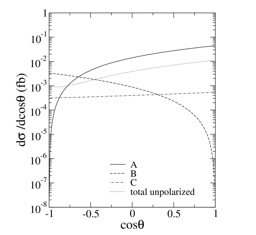
Figure 4: Differential cross section as a function of the scattering angle for $e^{+}e^{-}$ collisions. The following values of the parameters are used: $M_{1}=80,\;M_{2}=160,\;m_{\tilde{\ell}}=m_{\tilde{\nu}}=100$ GeV and $\Delta m^{2}=6000$ $\mbox{ GeV}^{2}$.

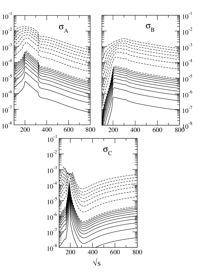
Figure 5: Total cross section (fb) as a function of $\sqrt{s}$ for $e^{+}e^{-}$ collisions for the three helicity amplitude. The parameters chosen are $M_{1}=80,\ M_{2}=160,\ m_{\tilde{\ell}}=m_{\tilde{\nu}}=100$ GeV. The solid lines correspond to $\Delta m^{2}$ increasing from $100$ GeV² to $900$ GeV² in steps of $100$. The dashed lines correspond to $\Delta m^{2}$ increasing from $1000$ to $8000$ GeV² in steps of $1000$.

The contributing amplitudes are (Appendix C.1):

$${\cal M}_{A} = {\cal M}(e^{+}_{R}e^{-}_{L}\to\ell^{-}_{L}e^{+}_{R}),$$ (26)

$${\cal M}_{B} = {\cal M}(e^{+}_{L}e^{-}_{R}\to\ell^{-}_{L}e^{+}_{R}),$$ (27)

$${\cal M}_{C} = {\cal M}(e^{+}_{L}e^{-}_{L}\to\ell^{-}_{L}e^{+}_{L}).$$ (28)

For each helicity amplitude the corresponding differential polarized cross section is shown in Fig. 4. The different behavior is easily understood in terms of helicity conservation at high energy. Amplitude ${\cal M}_{A}$ is peaked in the forward direction since it has a P-wave initial state with $J_{z}=+1$. Angular momentum conservation requires the right-handed positron to be emitted in the positive direction of the collision axis while the left-handed negative charged lepton must have its momentum in the opposite direction. Amplitude ${\cal M}_{B}$ is peaked in the backward direction as it is a P-wave scattering with $J_{z}=-1$. The right-handed positron must be emitted backward while the negative charged lepton is in the forward direction. Amplitude ${\cal M}_{C}$ has no virtual vector boson exchanged and is an S-wave ($J_{z}=0$) scattering. One expects therefore an almost flat, isotropic distribution.

The dominating contribution to the integrated unpolarized cross section comes from amplitude ${\cal M}_{A}$, which is an order of magnitude larger than ${\cal M}_{B}$ and two orders of magnitude larger than ${\cal M}_{C}$ in most of the phase space. Only for large scattering angles (backward direction) the amplitude ${\cal M}_{B}$ dominates and ${\cal M}_{A}$ is the smallest one. In Fig. 4 the dotted line corresponds to the unpolarized differential cross section (i.e. the inchoerent sum of the contributions of ${\cal M}_{A,B,C}$ averaged over the initial spins). It is worth to remark that in such circumstances the possibility of having polarized electron and positron beams would maximize the chances to observe these signals. Considering the unpolarized cross section corresponds essentially to calculating $\sigma_{unpol}\approx(1/4)\,\sigma(e^{+}_{R}e^{-}_{L}\to\ell^{-}_{L}e^{+}_{R})$.

Fig. 5 shows the cross section integrated over the scattering angle for the three helicity amplitude as a function of the center of mass energy $\sqrt{s}$ and for increasing values of the LFV parameter $\Delta m^{2}$. The presence of spikes is due to the onset of the absorptive part of the diagrams corresponding to thresholds of real particle pair production. For the values of masses used in Fig. 5 one expects thresholds effects at $\sim 200$ GeV for slepton pair production and $\sim 320$ GeV for gaugino pair production. This is evident for in $\sigma_{A}$ (upper-left panel) and $\sigma_{B}$ (upper-right panel). The shape is determined in the first case by the destructive interference among the two types of box graphs (with scalars and fermions on threshold) and by the value of $\Delta m^{2}$ inducing two distinct thresholds at $\tilde{m}^{2}\pm\Delta m^{2}$. $\sigma_{B}$ is determined only by penguin diagrams that give smaller contribution relative to the boxes. $\sigma_{C}$ receives contributions only from box diagrams: at threshold for sleptons production its value varies by orders of magnitude differently from the two other cases. This can be easily understood considering the threshold behavior of the cross section for sleptons pair production Peskin : defining $\beta$ the selectron velocity, the intermediate state of the amplitudes ${\cal M}_{A}$ and ${\cal M}_{B}$ correspond to the reactions $e^{-}_{L}e^{+}_{R}\to\tilde{e}^{-}_{L}\tilde{e}^{+}_{L}$ and $e^{-}_{R}e^{+}_{L}\to\tilde{e}^{-}_{L}\tilde{e}^{+}_{L}$ that near threshold behave like $\beta^{3}$ while amplitude ${\cal M}_{C}$ corresponds to the reaction $e^{-}_{L}e^{+}_{L}\to\tilde{e}^{-}_{L}\tilde{e}^{+}_{R}$ that at threshold behaves like $\beta$.

The cross section is peaked around $\sqrt{s}=2\tilde{m}_{L}$. In Fig. 6 $\sigma_{A}=\sigma(e_{R}^{+}e_{L}^{-}\to\ell^{-}_{L}e^{+}_{R})$ is shown as a function of $\delta_{LL}$ for $\sqrt{s}=2\tilde{m}_{L}$ and for different values of slepton and gaugino masses. Given an annual integrated luminosity $L_{0}$=100 $fb^{-1}$ a cross section of $10^{-2}$fb produces one signal event per year. Such an event rate is reached only for $M_{1}$ not larger than $\sim 200$ GeV and $\delta_{LL}\simeq{\cal O}(1)$. This hypothesis will be discussed in the next section.

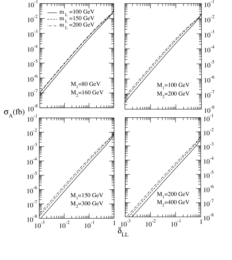
Figure 6: Total cross section for the amplitude A as a function of the dimensionless parameter $\delta_{LL}$ (see Eq. (20)) and for $\sqrt{s}=2\tilde{m}_{L}$. The values of the other parameters are given in the legends.

Moreover angular cuts in the forward direction are needed to suppress possible SM backgrounds and - since the largest values of the cross section correspond to small angles - the signal will be affected by such a cut. Therefore the observation of LFV in $e^{+}e^{-}$ collisons appears to be difficult unless $L_{0}$ is considerably larger than $10^{2}$ fb^-1/yr.

III.2 $\bm{e^{-}e^{-}}$ collisions

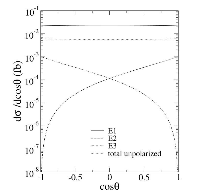
Figure 7: Differential cross section as a function of the scattering angle for $e^{-}e^{-}$ collisions. The choice of the parameters is the same as in Fig. 4.

The contributing amplitudes are (Appendix C.2)

$${\cal M}_{E1} = {\cal M}(e^{-}_{L}e^{-}_{L}\to\ell^{-}_{L}e^{-}_{L}),$$ (29)

$${\cal M}_{E2} = {\cal M}(e^{-}_{L}e^{-}_{R}\to\ell^{-}_{L}e^{-}_{R}),$$ (30)

$${\cal M}_{E3} = {\cal M}(e^{-}_{R}e^{-}_{L}\to\ell^{-}_{L}e^{-}_{R}).$$ (31)

The corresponding differential cross sections are plotted in Fig. 7. ${\cal M}_{E1}$ has $J_{z}=0$, is flat and forward-backward symmetric because of the antisymmtrizzation. ${\cal M}_{E2}$ and ${\cal M}_{E3}$ describe P-wave scattering with $J_{z}=+1$ and $J_{z}=-1$ respectively: in order to conserve angular momentum ${\cal M}_{E2}$ must be peaked in the forward direction while ${\cal M}_{E3}$ favours backward scattering. Both ${\cal M}_{E2}$ and ${\cal M}_{E3}$ are orders of magnitude smaller than ${\cal M}_{E1}$. The signal cross section is to a very good approximation given by the amplitude ${\cal M}_{E1}$. Since it is almost flat the angular integration will give a factor almost exactly equal to two. This again shows the importance of the option of having polarized beams. If both colliding electrons are left-handed one singles out the dominant helicity amplitude and a factor four is gained in the cross section relative to the unpolarized case. This may be important in view of the relatively small signal cross section one is dealing with.

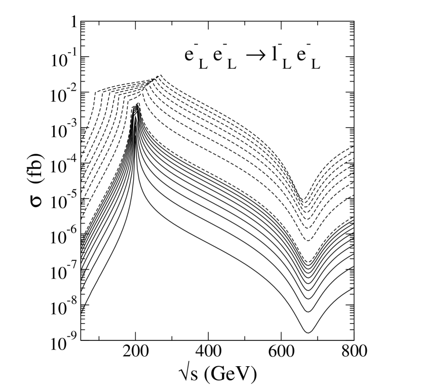
Figure 8: Total cross section of the dominant amplitude E1 as a function of $\sqrt{s}$ for $e^{-}e^{-}$ collisions. The choice of the parameters is the same as in Fig. 4.

In this case, due to the smaller number of diagrams, the analysis of the total cross section as a function of $\sqrt{s}$ is easier (see Fig. 8): the box diagrams dominate at $\sqrt{s}=2\tilde{m}_{L}$ where $\sigma$ changes of orders of magnitude giving a sharp peak that is smeared only by large values of $\Delta m^{2}$, while penguin diagrams give a substantial contribution only at higher energies. The reason is the same as for the $\sigma_{C}$ behaviour in the $e^{+}e^{-}$ case: the intermediate state $e^{-}_{L}e^{-}_{L}\to\tilde{e}^{-}_{L}\tilde{e}^{-}_{L}$ behaves like $\beta$, while the other two like $\beta^{3}$. Here the highest absolute value is due to the couplings and the constructive interference of boxes where both Binos and Winos can be exchanged.

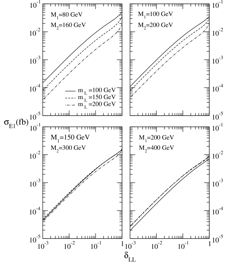
Figure 9: Total cross section for the amplitude E1 in function of the dimensionless parameter $\delta_{LL}$, see Eq. (20). The values of the other parameters are given in the legends. Each plotted line is calculated assuming $\sqrt{s}=2\tilde{m}_{L}$.

The dependence of $\sigma_{E1}$ on $\delta_{LL}$ is shown in Fig. 9. With SUSY masses not much larger than $\sim 200$ GeV the signal is of order ${\cal O}$(10^-2) fb for $\delta_{LL}>{\cal O}(10^{-1})$. Relative to the $e^{+}e^{-}$ case there are two important features: $(i)$ the cross section is practically angle independent so that it is insensitive to angular (or tranverse momentum) cuts; $(ii)$ the SM background - though not completely absent - can be easily controlled as will be shown in the next subsection.

III.2.1 $\bm{Background}$

The signal has the unique characteristic of a back to back high energy lepton pair. Sources of background were qualitatively discussed in Ref. Heusch .

Initial and final state radiation can be a source of background. An example is the OPAL event opal , although lepton pairs can hardly have the same kinematical feature of the signal. Other sources present multiparticle final states (at least six particles) and missing energy due to the presence of neutrino pairs.

The first type is given by reactions like $e^{-}e^{-}\to e^{-}e^{-}b^{*}{\bar{b}}^{*}$ that proceedes trough virtual photon fusion. The subsequent chain of weak deacys produces a final state with missing momentum, hadronic jets and opposite or same sign leptons, that however can be again separated using the clear kinematical topology of the signal.

A second type:

$$e^{-}e^{-}\to\nu_{e}\nu_{e}{W^{-}}^{*}{{W}^{-}}^{*}$$ (32)

$${W^{-}}^{*}{{W}^{-}}^{*}\to\ell^{-}{\bar{\nu}}_{\ell}\,{\ell^{-}}^{\prime}{\bar{\nu}}_{{\ell}^{\prime}}$$ (33)

with four neutrinos and a like sign-dilepton pair that can be of the same or different flavour. This appears to be the most dangerous background, as it produces two leptons and missing energy, and therefore it is analyzed in more detail. Moreover, to the best of our knowledge, it has not been previously considered in the literature. Fig. 10 shows the total cross section $e^{-}e^{-}\to\nu_{e}\nu_{e}{W^{-}}{{W}^{-}}$ calculated with the CompHEP package comphep , that allows to compute numerically the $17$ Feynman diagrams contributing at tree level. Above the threshold for $W^{-}W^{-}$ gauge boson production the cross section rises rapidly by orders of magnitude, becoming almost constant at high energies. In the region $\sqrt{s}\simeq 250-400$ GeV it increases from $10^{-2}$ fb to $1$ fb. In order to get an estimate of the cross section for the six particle final state process, the cross section $\sigma(e^{-}e^{-}\to{W^{-}}{{W}^{-}}\nu\nu)$ has to be multiplied by the branching ratio of the leptonic decays of the two gauge bosons, $\simeq 10\%$, so that $\sigma_{Background}\simeq 10^{-4}-10^{-2}$ fb, and it is at the level of the signal. However the kinematical configuration of the final state leptons is completely different. Fig. 10 (upper-right) shows the angular distribution of the gauge bosons which is peaked in the forward and backward directions so that the leptons produced in the $W$ gauge boson decay are emitted preferentially along the collsion axis.

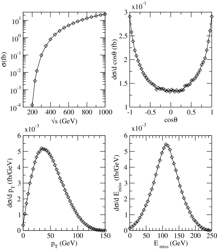
Figure 10: Total cross section and distributions for $e^{-}e^{-}\to W^{-}W^{-}\nu\nu$ Upper-left figure: total cross section as a function of $\sqrt{s}$. Upper-right: angular distribution for a $W^{-}$ where $\theta$ is the angle among the collision axis and the boson momentum. Bottom-left: distribution of the transverse momentum of $W^{-}$. Bottom-right: energy distribution of the two neutrinos. All distributions are calculated with $\sqrt{s}=300$ GeV.

In addition their tansverse momenta will be softer compared to that of the signal: Fig. 10 (bottom-left panel) shows that the transverse momenta distribution of the gauge bosons is peaked at $p^{P}_{T}=(\sqrt{s}/2-M_{W})/2\simeq 35$ GeV for $\sqrt{s}=300$ GeV. Consequentely the lepton distributions will be peaked at $p^{P}_{T}/2\simeq 17.5$ GeV. The missing energy due to the undetected neutrinos (Fig. 10, bottom-right panel) can be as large as $\simeq\sqrt{s}-2M_{W}$. This distribution should be convoluted with that of the neutrinos produced in the gauge boson decay. Therefore it can be safely concluded that it will be possible to control this background because, with reasonable cuts on the transverse momenta and missing energy, it will be drastically reduced, while - as mentioned above - these cuts will not affect significantly the signal.

IV Comparison with rare lepton radiative decays

The main result of the calculations presented in the previous sections is that, as it can be inferred from Fig. 9, the phenomenological points of the SUSY parameter space corresponding to gaugino masses $(M_{1},\;M_{2})=(80,\;160)$ GeV or $(100,\;200)$ GeV and to slepton masses $m_{L}=100-200$ GeV and $\delta_{LL}>10^{-1}$ (which implies $\Delta m^{2}>10^{3}$ GeV²) can give in the $e^{-}e^{-}$ mode a detectable LFV signal ($e^{-}e^{-}\to\ell^{-}e^{-}$) although at the level of ${\cal O}(1-25)$ events/yr with ${L}_{0}=100$ fb^-1. Higher sensitivity to the SUSY parameter space could be obtained with larger $L_{0}$. It is interesting to note that this light sparticles spectrum that is promising for collider discovery, is also preferred by the electroweak data fit. In Ref. Altarelli it is shown that light sneutrinos, charged left sleptons and light gauginos improve the agreement among the electroweak precision measurements and the lower bounds on the Higgs mass.

On the other hand the experimental bounds on rare lepton decays set constraints on the LFV violating paramters $\Delta\tilde{m}^{2}$ or $\delta_{LL}$: the constraints in Eq. (3) define an allowed (and an excluded) region in the plane ($\delta_{LL},m_{L}$) which are computed using the formulas given in Ref. hisa2 (adapted to our model) for the LFV radiative lepton decays. These regions have to be compared with those satisfying the “discovery” condition

$$L_{0}\sigma(\delta_{LL},m_{L})\geq 1.$$ (34)

Such a comparison is shown in Fig. 11 from which it emerges that: ($i$) For the $e^{-}e^{-}\to\ell^{-}e^{-}$ process there is an observable signal in the upper left corner of the ($\delta_{LL},m_{L}$) plane. The extension of this region depends on $L_{0}$. ($ii$) The bound from $\tau\to e\gamma$ does not constrain the region of the ($\delta_{LL},m_{L}$) plane compatible with an observable LFV signal and therefore the reaction $e^{-}e^{-}\to\tau^{-}e^{-}$ could produce a detectable signal whithin the highlighted regions of the parameter space (upper-left regions in the ($\delta_{LL},m_{L}$) plane). ($iii$) As regards the constraints from the $\mu\to e\gamma$ decay the allowed region in the ($\delta_{LL},m_{L}$) plane is shown by the circular dark dots (red with colour): the process $e^{-}e^{-}\to\mu^{-}e^{-}$ is observable only in a small section of the parameter space since the allowed region from the $\mu\to e\gamma$ decay almost does not overlap with the collider “discovery” region except for a very small fraction in the case of gaugino masses ($M_{1}=80$ GeV and $M_{2}=160$ GeV). The compatibility of values of $\delta_{LL}\approx 1$ is due to a cancellation among the diagrams that describe the $\ell\to\ell^{\prime}\gamma$ decay in particular points of the parameter space illa .

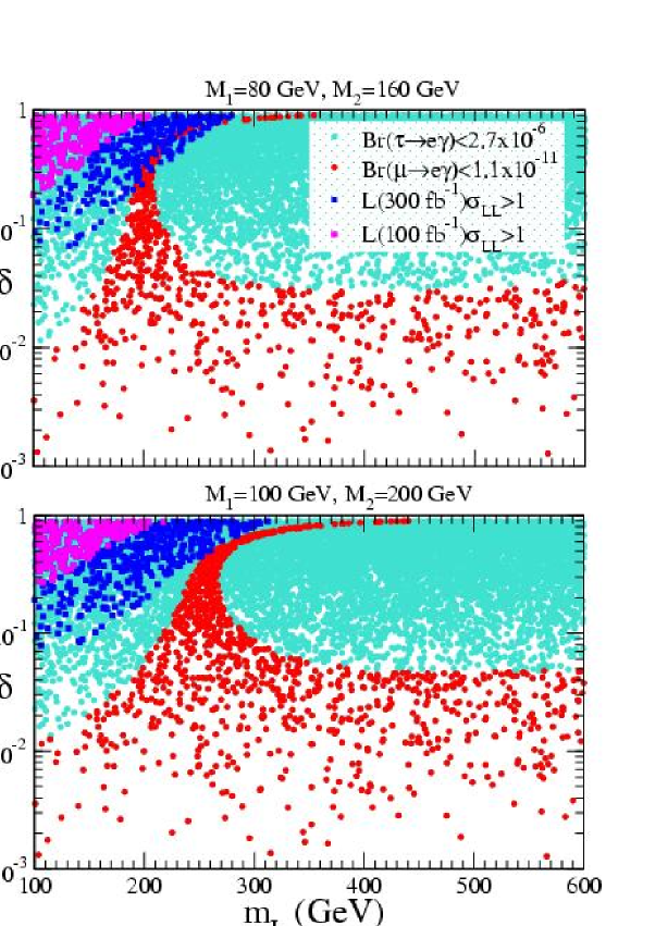
Figure 11: Scatter plot in the plane ($\delta_{LL},m_{L}$) of: (a) the experimental bounds from $\mu\to e\gamma$ and $\tau\to\mu\gamma$ (allowed regions with circular dots); (b) regions where the signal can give at least one event with two different values of integrated luminosity (squared dots), for two sets of gaugino masses. Each signal point is calculated at $\sqrt{s}=2\tilde{m}_{L}$.

As regards the radiative mechanism that generates the off-diagonal elements in mSUGRA models (as discussed in Sec. II) one should check if this mechanism may generate large values of $\Delta m^{2}$. The answer is yes, at least for some particular scenario of neutrino masses and mixing. It is well known that any ‘bottom-up’ approach that reconstructs the $Y_{\nu}$ from the see-saw mechanism and neutrino masses and mixings is ambiguous up to a complex, orthogonal matrix $R$  casas . Usually this matrix is taken to be real or identical to the unit matrix. However in Ref. pascoli it is shown that in the case of a quasi-degenerate neutrino mass spectrum $R$ being complex allows for values of $\Delta m^{2}$ being larger by 5-8 orders of magnitude relative to the case of $R$ being real or the unit matrix. In this case one has pascoli

$$|(Y^{\dagger}_{\nu}Y_{\nu})_{13}|^{2}\simeq\frac{M^{2}_{R}m^{2}_{\nu}}{v^{4}}\times{\cal O}(0.1-1.0).$$ (35)

Choosing for example $M_{R}=2\cdot 10^{14}$ GeV, $M_{GUT}=2\cdot 10^{16}$ GeV, $m_{\nu}=0.3$ eV, $v=174$ GeV in Eq. (35) and $a_{0}=0$, $m_{0}=150$ GeV in Eq. (10) $\Delta m^{2}$ varies in the range $2400-7800$ GeV², i.e. with $100\ \hbox{GeV}\leq m_{L}\leq 200\ \hbox{GeV}$, $\delta_{LL}$ is in the range ($0.06-0.78$).

V Summery and Conclusions

The search at lepton colliders of lepton flavour and lepton number violating signal is complementary to the search for rare leptons decays. The next generation of linear colliders will offer the opportunity to look for reactions like $e^{\pm}e^{-}\to\ell^{\pm}e^{-}\;(\ell=\mu,\tau)$ at energies well above the $Z$ peak resonance. Upper bounds on the cross sections for these processes at the highest energies reached by LEP, $189\;\mbox{GeV}\leq\sqrt{s}\leq 209\;\mbox{GeV}$, where given by the OPAL collaboration, Eq. (6).

In this paper the reactions $e^{\pm}e^{-}\to\ell^{\pm}e^{-}\;(\ell=\mu,\tau)$ induced by sleptons mixing in R-parity conserving supersymmetry have been studied. The reactions proceed through loop diagrams (box and penguin type) involving sleptons, neutralinos and charginos. The amplitudes have been evaluated in the helicity basis and the loop integrals are calculated numerically. The resulting cross sections exhibit the well known threshold enhancement for center of mass energies corresponding to pair production of supersymmetric particles. In particular due to the dominance of the $(s,t)$-channel box diagrams with sleptons on the threshold in the intermediate state, the LFV cross section reaches its maximum value at the energy corresponding to the threshold for sleptons pair production both in $e^{+}e^{-}$ and $e^{-}e^{-}$ collisions.

The $e^{-}e^{-}$ option with left-polarized beams stands better chances to provide a detectable signal. A comparison with present experimental bounds on radiative lepton decays shows that an observable ($e^{-}e^{-}\to\tau^{-}e^{-}$) signal is compatible with the non observation of the decay $\tau\to e\gamma$ giving some tens of events with an integrated luminosity of 100 fb^-1. On the contrary the more restrictive constraints from the non-observation of $\mu\to e\gamma$ make the search of $e^{-}e^{-}\to\mu^{-}e^{-}$ unrealistic unless the integrated luminosity is very large. It has been shown that the Standard Model background is low and can be easily suppressed using that the signal final state consists of two back to back high energy leptons of different flavour with no missing energy. The observation $e^{+}e^{-}$ in collisions will be more difficult because of smaller cross sections.

Appendix A Lagrangian and couplings

The interaction lagrangians in the gauge basis for superparticles in the notation of Ref. Haber :

(a)Lepton-chargino-sneutrino:

$${\cal L}=O^{\tilde{W}}_{\tilde{\nu}}\overline{\ell}P_{R}\tilde{W}\tilde{\nu}+h.c.,$$ (36)

with coupling $O^{\tilde{W}}_{\tilde{\nu}}=-g$.

(b) Lepton-neutralino-slepton:

$${\cal L} = (O^{\tilde{W}^{3}}_{\tilde{L}}\overline{\ell}P_{R}\tilde{W}^{3}\tilde{L}+O^{\tilde{B}}_{\tilde{L}}\overline{\ell}P_{R}\tilde{B}\tilde{L}+O^{\tilde{B}}_{\tilde{R}}\overline{\ell}P_{L}\tilde{B}\tilde{R})$$ (37)

$$+ h.c.,$$ (38)

with couplings given by $O^{\tilde{W}^{3}}_{\tilde{L}}=\frac{g}{\sqrt{2}}$, $O^{\tilde{B}}_{\tilde{L}}=\frac{g}{\sqrt{2}}t_{W}$, $O^{\tilde{B}}_{\tilde{R}}={\sqrt{2}}gt_{W}$ and $\tilde{L}\equiv\tilde{\ell}_{L}$, $\tilde{R}\equiv\tilde{\ell}_{R}$.

(c) Lepton-lepton-vector boson:

$${\cal L}=\sum_{V=\gamma,Z^{0}}V_{\mu}\overline{\ell}\gamma^{\mu}(O_{V}^{L}P_{L}+O_{V}^{R}P_{R})\ell$$ (39)

where $O_{Z^{0}}^{R}=-gs_{W}t_{W}$, $O_{Z^{0}}^{L}=+\frac{g}{c_{W}}(\frac{1}{2}-s^{2}_{W})$, $O^{L}_{\gamma}=O^{R}_{\gamma}=e$.

(d) Slepton-slepton-vector boson:

$${\cal L}=iO_{V}^{\tilde{L}\tilde{L}}V_{\mu}\tilde{L}^{*}\overleftrightarrow{\partial}^{\mu}\tilde{L},$$ (40)

with $O^{\tilde{\ell}\tilde{\ell}}_{\gamma}=e$, $O^{\tilde{\ell}\tilde{\ell}}_{Z^{0}}=g\frac{g}{c_{W}}(\frac{1}{2}-s^{2}_{W})$, $O^{\tilde{\nu}\tilde{\nu}}_{Z^{0}}=-\frac{g}{2c_{W}}$.

(e) Chargino-chargino-vector boson:

$${\cal L}=O_{V}^{\tilde{W}}V_{\mu}\overline{\tilde{W}}\gamma^{\mu}\tilde{W}$$ (41)

with $O_{\gamma}^{\tilde{W}}=-e$, $O_{Z^{0}}^{\tilde{W}}=-gc_{W}$.

Appendix B Numerical tools

B.1 Spinor products

Here the basic formulas used in the computation of helicity amplitudes are given. More details and proofs are given in Ref. kleiss . The spinor products satisfy exchange relations:

$$\begin{array}[]{ccc}S(p_{a},p_{b})=-S(p_{b},p_{a}),&T(p_{a},p_{b})=-T(p_{b},p_{a}),\\ S(p_{a},p_{b})=T^{*}(p_{b},p_{a}),&T(p_{a},p_{b})=S^{*}(p_{a},p_{b}),\\ |S(p_{b},p_{a})|^{2}=2p_{a}\cdot p_{b},&|T(p_{a},p_{b})|^{2}=2p_{a}\cdot p_{b}.\end{array}$$ (42)

The necessary relations to write the amplitudes in terms of spinor products are the Chisholm identities:

$$\left[\overline{u}_{\lambda}(p_{a}){\gamma^{\mu}}u_{\lambda}(p_{b})\right]\gamma_{\mu}=$$ (43)

$$2\left[u_{\lambda}(p_{b})\overline{u}_{\lambda}(p_{a})+u_{-\lambda}(p_{a})\overline{u}_{-\lambda}(p_{b})\right],$$ (44)

$$p/=u_{R}(p)\overline{u}_{R}(p)+u_{L}(p)\overline{u}_{L}(p).$$ (45)

where $\lambda=L,R$ indicates the helicity of the spinor. The external momenta are parametrized in terms of the Mandelstam variable $s$ and the scattering angle in the center of mass frame:

$$p_{1} = \frac{\sqrt{s}}{2}(1,0,0,1),$$ (46)

$$p_{2} = \frac{\sqrt{s}}{2}(1,0,0,-1),$$ (47)

$$p_{3} = \frac{\sqrt{s}}{2}(1,-\sin{\theta},0,-\cos{\theta}),$$ (48)

$$p_{4} = \frac{\sqrt{s}}{2}(1,\sin{\theta},0,\cos{\theta}).$$ (49)

The spinor products are determined by the components of these four momenta in the following way:

$$S(p_{a},p_{b}) = (p_{a}^{z}+ip_{a}^{x})\sqrt{\frac{p_{b}^{0}-p_{b}^{y}}{p_{a}^{0}-p_{a}^{y}}}$$ (50)

$$- (p_{b}^{z}+ip_{b}^{x})\sqrt{\frac{p_{a}^{0}-p_{a}^{y}}{p_{b}^{0}-p_{b}^{y}}},$$ (51)

and $T(p_{a},p_{b})$ is easily deduced by ralations (42). Using Eq. (49) and Eq. (51) it is easy to see that the relations (42) are satisfied. In the case of $2\to 2$ scattering, with the momenta given in Eq. (49), the preceding expressions simplifies to:

$$S(p_{a},p_{b}) = (p_{a}^{z}-p_{b}^{z})+i(p_{a}^{x}-p_{b}^{x}),$$ (52)

$$T(p_{a},p_{b}) = (p_{b}^{z}-p_{a}^{z})-i(p_{b}^{x}-p_{a}^{x}),$$ (53)

and product of spinor products are directly related to $s,t,u$. For example one has:

$$S(p_{1},p_{3})T(p_{4},p_{2}) = -\frac{s}{2}(1+\cos{\theta})=u,$$ (54)

$$S(p_{1},p_{4})T(p_{3},p_{2}) = -\frac{s}{2}(1-\cos{\theta})=t,$$ (55)

$$S(p_{1},p_{2})T(p_{4},p_{3}) = se^{i\theta}.$$ (56)

B.2 Tensor integral decomposition

The loop integrals are evaluated numerically with the package LoopTools looptools . Here we report the definitions and the decomposition for two, three and four point tensor functions.

$$B_{\mu} = \int\frac{d^{4}q}{i\pi^{2}}\frac{q_{\mu}}{N_{1}N_{2}},$$ (57)

$$C_{\mu;\alpha\beta} = \int\frac{d^{4}q}{i\pi^{2}}\frac{q_{\mu};q_{\alpha}{q_{\beta}}}{N_{1}N_{2}N_{3}},$$ (58)

$$D_{\mu;\alpha\beta} = \int\frac{d^{4}q}{i\pi^{2}}\frac{q_{\mu};q_{\alpha}{q_{\beta}}}{N_{1}N_{2}N_{3}N_{4}},$$ (59)

are expressed as:

$$B_{\mu} = k_{1\mu}B_{1}$$ (60)

$$C_{\mu} = \sum^{2}_{i=1}{k_{i}}_{\mu}C_{i},$$ (61)

$$C_{\mu\nu} = g_{\mu\nu}C_{00}+\sum^{2}_{i,j=1}{k_{i}}_{\mu}{k_{j}}_{\nu}C_{ij}$$ (62)

$$D_{\mu} = \sum^{3}_{i=1}{k_{i}}_{\mu}D_{i},$$ (63)

$$D_{\mu\nu} = g_{\mu\nu}D_{00}+\sum^{3}_{i,j=1}{k_{i}}_{\mu}{k_{j}}_{\nu}D_{ij},$$ (64)

where the $k_{i}$’s are sums of external momenta appearing in the loops propagators as reported in Fig. 12:

$$q_{1} = q+k_{1}=q+p_{1},$$ (65)

$$q_{2} = q+k_{2}=q+p_{1}+p_{2},$$ (66)

$${q_{2}}_{u,t} = q+p_{1}-p_{3},$$ (67)

$$q_{3} = q+k_{3}=q+p_{4},$$ (68)

$${q_{3}}_{u} = q+p_{3},$$ (69)

$$q_{1}^{\prime} = q+k_{1}^{\prime}=q+p_{4},$$ (70)

$$q_{2}^{\prime} = q+k_{2}^{\prime}=q+p_{3}+p_{4},$$ (71)

$${{q_{1}}_{t}}^{\prime} = q+p_{3},$$ (72)

$${{q_{2}}_{t}}^{\prime} = q+p_{3}-p_{2},$$ (73)

$$q^{\prime} = q-p_{3}$$ (74)

and the mass and Mandelstam variables dependence for a generic two, three, four point function and for the various topologies of graphs corresponding to the kinematical channels are:

$$D_{a} = D(0,0,0,0,s,t,m^{2}_{q},m^{2}_{q_{1}},m^{2}_{q_{2}},m^{2}_{q_{3}}),$$ (75)

$$D_{b} = D(0,0,0,0,s,u,m^{2}_{q},m^{2}_{q_{1}},m^{2}_{q_{2}},m^{2}_{q_{3}}),$$ (76)

$$D_{c} = D(0,0,0,0,u,t,m^{2}_{q},m^{2}_{q_{1}},m^{2}_{q_{2}},m^{2}_{q_{3}}),$$ (77)

$$C_{d} = C(0,0,s,m^{2}_{q^{\prime}},m^{2}_{q_{1}^{\prime}},m^{2}_{q_{2}^{\prime}}),$$ (78)

$$C_{e} = C(0,0,t,m^{2}_{q^{\prime}},m^{2}_{q_{1}^{\prime}},m^{2}_{q_{2}^{\prime}}),$$ (79)

$$B_{f} = B(m^{2}_{q},m^{2}_{q^{\prime}}).$$ (80)

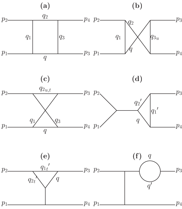
Figure 12: Definition of virtual momenta for kinematics and tensor integral decomposition.

Appendix C Helicity amplitudes

C.1 $\bm{e^{+}e^{-}}$ collisions

The amplitudes are given assuming that the negative charged final leptons has changed flavour. The other possibility is taken into account simply multiplyng the total cross section by two. The non-zero helicity amplitudes are found to be:

A: $e^{+}_{R}e^{-}_{L}\to\ell^{-}_{L}e^{+}_{R}$

For clarity, graphs are grouped according to the virtual particles present in the boxes that can be produced in $e^{+}e^{-}$ collisions:
1.Virtual selectrons pair:
There are four box diagrams with all the possible $\tilde{B}$ and $\tilde{W}$ assignament in the neutralino lines in Figs. 1a, 1b:

$${\cal M}_{A,1}^{\Box} = \sum_{i,i^{\prime}=\tilde{B},\tilde{W^{0}}}(O^{i})^{2}(O^{i^{\prime}})^{2}T(p_{1},p_{3})S(p_{4},p_{2})$$ (81)

$$\times \left\{2D^{ii^{\prime}}_{00}(s,t)+T(p_{1},p_{4})S(p_{4},p_{1})D_{13}^{i,i^{\prime}}(s,t)\right.$$ (82)

$$- \left.m_{i}m_{i^{\prime}}D_{0}^{ii^{\prime}}(u,t)\right\}.$$ (83)

The terms depending on $(u,t)$ come from the crossed box diagrams due to the Majorana nature of neutralinos. Contribution from $s$ and $t$ channel penguins, Figs. 2a, 2b and the corresponding external legs corrections, Fig. 2d, give:

$${\cal M}_{A,1}^{\triangle} = 2T(p_{1},p_{3})S(p_{4},p_{2})$$ (84)

$$\times \left\{\sum_{V,i}D_{V}(s)\left[(O^{i})^{2}O_{V}^{\tilde{\ell}\tilde{\ell}}O^{V}_{L}2C_{00}(s)\right.\right.$$ (85)

$$- \left.(O^{i})^{2}(O^{V}_{L})^{2}(B_{0}+B_{1})\right]$$ (86)

$$- \left.\sum_{V,i}D_{V}(t)\left[(O^{i})^{2}O_{V}^{\tilde{\ell}\tilde{\ell}}O^{V}_{L}2C_{00}(t)\right.\right.$$ (87)

$$- \left.\left.(O^{i})^{2}(O^{V}_{L})^{2}(B_{0}+B_{1})\right]\right\}$$ (88)

The photon and $Z^{0}$ propagators are given by $D_{V}(s)=-i/(s-M^{2}_{V}+iM_{V}\Gamma_{V})$ ($V=\gamma,Z)$ for the $s$-channel, while no immaginary part is present in the denominator for $t$ and $u$ channels.

2. Virtual sneutrinos pair:
The box diagrams in Fig. 1c reads:

$${\cal M}_{A,2}^{\Box} = ({O^{\tilde{W}}_{\tilde{\nu}}})^{4}T(p_{1},p_{3})S(p_{4},p_{2})\left\{2D_{00}(s,t)\right.$$ (89)

$$+ \left.T(p_{1},p_{4})S(p_{1},p_{4})D_{13}(s,t)\right\},$$ (90)

while the penguins of Figs. 2b, 2e:

$${\cal M}_{A,2}^{\triangle} = 2T(p_{1},p_{3})S(p_{4},p_{2})$$ (91)

$$\times \left\{D_{Z}(s)\left[({O^{\tilde{W}}_{\tilde{\nu}}})^{2}O_{Z}^{\tilde{\nu}\tilde{\nu}}O^{Z}_{L}2C_{00}(s)\right.\right.$$ (92)

$$- \left.({O^{\tilde{W}}_{\tilde{\nu}}})^{2}(O^{Z}_{L})^{2}(B_{0}+B_{1})\right]$$ (93)

$$- \left.D_{Z}(t)\left[({O^{\tilde{W}}_{\tilde{\nu}}})^{2}O_{Z}^{\tilde{\nu}\tilde{\nu}}O^{Z}_{L}2C_{00}(t)\right.\right.$$ (94)

$$- \left.\left.({O^{\tilde{W}}_{\tilde{\nu}}})^{2}(O^{Z}_{L})^{2}(B_{0}+B_{1})\right]\right\}$$ (95)

The amplitudes present the same structure of those in case 1.

3. Virtual chargino pair:

The box diagram in Fig. 1d:

$${\cal M}_{A,3}^{\Box} = ({O^{\tilde{W}}_{\tilde{\nu}}})^{4}T(p_{1},p_{3})S(p_{2},p_{4})\left\{2D_{00}(s,t)\right.$$ (96)

$$+ \left.T(p_{1},p_{2})S(p_{1},p_{2}){\cal D}(s,t)\right\}.$$ (97)

where $k,l=s,t,u$ and

$${\cal D}(k,l)=[D_{12}(k,l)+D_{22}(k,l)+D_{23}(k,l)+D_{2}(k,l)],$$

The penguin diagrams in Figs. 2c, 2e give:

$${\cal M}_{A,3}^{\triangle} = 2T(p_{1},p_{3})S(p_{4},p_{2})$$ (98)

$$\times \left\{\sum_{V=\gamma,Z^{0}}D_{V}(s)\left[({O^{\tilde{W}}_{\tilde{\nu}}})^{2}O_{V}^{\tilde{W}}O^{V}_{L}{\cal C}(s)\right.\right.$$ (99)

$$- \left.\left.({O^{\tilde{W}}_{\tilde{\nu}}})^{2}(O^{\gamma}_{L})^{2}(B_{0}+B_{1})\right]\right.$$ (100)

$$- \left.\sum_{V=\gamma,Z^{0}}D_{V}(t)\left[({O^{\tilde{W}}_{\tilde{\nu}}})^{2}O_{V}^{\tilde{W}}O^{V}_{L}{\cal C}(t)\right.\right.$$ (101)

$$- \left.\left.({O^{\tilde{W}}_{\tilde{\nu}}})^{2}(O^{\gamma}_{L})^{2}(B_{0}+B_{1})\right]\right\}$$ (102)

where $k=s,t,u$ and

$${\cal C}(k) = \left\{C_{0}(k)m^{2}_{\tilde{W}}\right.$$

$$- \left.\left[2C_{00}(k)+k(C_{2}(k)+C_{12}(k)+C_{22}(k))\right]\right\}.$$

4. Virtual neutralino pair:
There are four box diagrams with left-slepton and all possible combinations of Bino and neutral Wino in the loop of Figs. 1e, 1f with left sleptons exchanged:

$${\cal M}_{A,4}^{\Box} = \sum_{i,i^{\prime}}(O^{i})^{2}(O^{i^{\prime}})^{2}T(p_{1},p_{3})S(p_{2},p_{4})$$ (104)

$$\times \left\{2D^{ii^{\prime}}_{00}+T(p_{1},p_{2})S(p_{1},p_{2}){\cal D}^{i,i^{\prime}}(s,t)\right.$$ (105)

$$- \left.m_{i}m_{i^{\prime}}D_{0}^{ii^{\prime}}(s,u)\right\}$$ (106)

Note that there is no penguin contribution to this channel in the $\tilde{B},\tilde{W}^{0}$ basis. The amplitudes ${\cal M}^{\Box}_{A,3}$ and ${\cal M}^{\Box}_{A,4}$ have a minus sign relative to the other amplitudes, because $T(p_{1},p_{3})S(p_{2},p_{4})=-T(p_{1},p_{3})S(p_{4},p_{2})$, see Eq. (42). Its origin is due to the fact that once one fixes the order of the spinors, the two different topologies of box diagrams need an odd number of permutation of fermion fields to bring them in the same order. The same holds for the relative sign between $s$ and $t$ channel penguins.

B: $e^{+}_{L}e^{-}_{R}\to\ell^{-}_{L}e^{+}_{R}$

This differs from the previous by the exchange of initial state helicity: only the penguin diagrams contribute and the amplitudes are obtained selecting the $O^{\gamma,Z}_{R}P_{R}$ operator in the lepton-lepton-vector boson vertex.

$${\cal M}_{B,1}^{\triangle} = 2T(p_{1},p_{4})S(p_{3},p_{2})$$ (107)

$$\times \left\{\sum_{V,i}D_{V}(s)\left[(O^{i})^{2}O_{V}^{\tilde{\ell}\tilde{\ell}}O^{V}_{R}2C_{00}(s)\right.\right.$$ (108)

$$- \left.\left.(O^{i})^{2}(O^{V}_{R})^{2}(B_{0}+B_{1})\right]\right.$$ (109)

$$- \left.\sum_{V,i}D_{V}(t)\left[(O^{i})^{2}O_{V}^{\tilde{\ell}\tilde{\ell}}O^{V}_{R}2C_{00}(t)\right.\right.$$ (110)

$$- \left.\left.(O^{i})^{2}(O^{V}_{R})^{2}(B_{0}+B_{1})\right]\right\}$$ (111)

$${\cal M}_{B,2}^{\triangle} = 2T(p_{1},p_{4})S(p_{3},p_{2})$$ (112)

$$\times \left\{D_{Z}(s)\left[({O^{\tilde{W}}_{\tilde{\nu}}})^{2}O_{Z}^{\tilde{\nu}\tilde{\nu}}O^{Z}_{R}2C_{00}(s)\right.\right.$$ (113)

$$- \left.\left.({O^{\tilde{W}}_{\tilde{\nu}}})^{2}(O^{Z}_{R})^{2}(B_{0}+B_{1})\right]\right.$$ (114)

$$- \left.D_{Z}(t)\left[({O^{\tilde{W}}_{\tilde{\nu}}})^{2}O_{Z}^{\tilde{\nu}\tilde{\nu}}O^{Z}_{R}2C_{00}(t)\right.\right.$$ (115)

$$- \left.\left.({O^{\tilde{W}}_{\tilde{\nu}}})^{2}(O^{Z}_{R})^{2}(B_{0}+B_{1})\right]\right\}$$ (116)

$${\cal M}_{B,3}^{\triangle} = 2T(p_{1},p_{4})S(p_{3},p_{2})$$ (117)

$$\times \left\{\sum_{V=\gamma,Z^{0}}D_{V}(s)\left[({O^{\tilde{W}}_{\tilde{\nu}}})^{2}O_{V}^{\tilde{W}}O^{V}_{R}{\cal C}(s)\right.\right.$$ (118)

$$- \left.\left.({O^{\tilde{W}}_{\tilde{\nu}}})^{2}(O^{\gamma}_{R})^{2}(B_{0}+B_{1})\right]\right.$$ (119)

$$- \left.\sum_{V=\gamma,Z^{0}}D_{V}(t)\left[({O^{\tilde{W}}_{\tilde{\nu}}})^{2}O_{V}^{\tilde{W}}O^{V}_{R}{\cal C}(t)\right.\right.$$ (120)

$$- \left.\left.({O^{\tilde{W}}_{\tilde{\nu}}})^{2}(O^{\gamma}_{R})^{2}(B_{0}+B_{1})\right]\right\}$$ (121)

C: $e^{+}_{L}e^{-}_{L}\to\ell^{-}_{L}e^{+}_{L}$

The box diagram in Figs. 1e, 1f with the right-handed selectron and the Binos in the neutralinos lines contributes:

$${\cal M}_{C,1}^{\Box} = ({O^{\tilde{B}}_{\tilde{L}}})^{2}({O^{\tilde{B}}_{\tilde{R}}})^{2}\left\{S(p_{1},p_{2})T(p_{3},p_{4})2D_{00}(s,t)\right.$$ (122)

$$+ \left.S(p_{1},p_{2})T(p_{2},p_{4})T(p_{3},p_{1})S(p_{1},p_{2}){\cal D}(s,t)\right.$$ (123)

$$- \left.S(p_{1},p_{2})T(p_{3},p_{4})\left[2D_{00}(s,u)\right.\right.$$ (124)

$$+ \left.\left.S(p_{1},p_{4})T(p_{1},p_{4})D_{13}(s,u)\right]\right\}$$ (125)

The box diagrams in Figs. 1g, 1h:

$${\cal M}_{C,2}^{\Box} = ({O^{\tilde{B}}_{\tilde{L}}})^{2}({O^{\tilde{B}}_{\tilde{R}}})^{2}S(p_{1},p_{2})T(p_{3},p_{4})$$ (126)

$$\times \left\{m_{\tilde{B}}^{2}D_{0}(s,t)-2D_{00}(u,t)\right.$$ (127)

$$+ \left.S(p_{1},p_{4})T(p_{1},p_{4})D_{13}(u,t)\right\}$$ (128)

C.2 $\bm{e^{-}e^{-}}$ collisions

The helicity amplitudes are:

E1: $e^{-}_{L}e^{-}_{L}\to\ell^{-}_{L}e^{-}_{L}$

Four box diagrams of the kind given in Fig. 3a with left sleptons and the box in Fig. 3b with charginos:

$${\cal M}^{\Box}_{E1} =\sum_{i,i^{\prime}}(O^{i})^{2}(O^{i^{\prime}})^{2}S(p_{1},p_{2})T(p_{4},p_{3})$$ (129)

$$\times \left\{m_{i}m_{i^{\prime}}D_{0}^{i}(s,t)+2D_{00}^{ii^{\prime}}(u,t)\right.$$ (130)

$$- \left.S(p_{4},p_{1})T(p_{4},p_{1})D_{13}^{ii^{\prime}}(u,t)\right\}$$ (131)

$$+ ({O^{\tilde{W}}_{\tilde{\nu}}})^{4}\left[2D^{c}_{00}(u,t)+S(p_{4},p_{1})T(p_{4},p_{1})D^{c}_{13}(u,t)\right]$$ (132)

$$- {\cal M}(p_{1}\leftrightarrow p_{2},u\leftrightarrow t)$$ (133)

Penguin diagrams in $t$ and $u$ channels, with left couplings with gauge bosons:

$${\cal M}_{E1,1}^{\triangle} = 2S(p_{2},p_{1})T(p_{4},p_{3})$$ (134)

$$\times \left\{\sum_{V,i}D_{V}(t)\left[(O^{i})^{2}O_{V}^{\tilde{\ell}\tilde{\ell}}O^{V}_{L}2C_{00}(t)\right.\right.$$ (135)

$$- \left.\left.(O^{i})^{2}(O^{V}_{L})^{2}(B_{0}+B_{1})\right]\right.$$ (136)

$$- \left.\sum_{V,i}D_{V}(u)\left[(O^{i})^{2}O_{V}^{\tilde{\ell}\tilde{\ell}}O^{V}_{L}2C_{00}(u)\right.\right.$$ (137)

$$- \left.\left.(O^{i})^{2}(O^{V}_{L})^{2}(B_{0}+B_{1})\right]\right\}$$ (138)

$$- {\cal M}(p_{1}\leftrightarrow p_{2},u\leftrightarrow t)$$ (139)

$${\cal M}_{E1,2}^{\triangle} = 2S(p_{2},p_{1})T(p_{4},p_{3})$$ (140)

$$\times \left\{D_{V}(t)\left[({O^{\tilde{W}}_{\tilde{\nu}}})^{2}O_{V}^{\tilde{\nu}\tilde{\nu}}O^{Z}_{L}2C_{00}(t)\right.\right.$$ (141)

$$- \left.\left.(O^{i})^{2}(O^{Z}_{L})^{2}(B_{0}+B_{1})\right]\right.$$ (142)

$$- \left.D_{Z}(u)\left[({O^{\tilde{W}}_{\tilde{\nu}}})^{2}O_{Z}^{\tilde{\nu}\tilde{\nu}}O^{Z}_{L}2C_{00}(u)\right.\right.$$ (143)

$$- \left.\left.({O^{\tilde{W}}_{\tilde{\nu}}})^{2}(O^{Z}_{L})^{2}(B_{0}+B_{1})\right]\right\}$$ (144)

$$- {\cal M}(p_{1}\leftrightarrow p_{2},u\leftrightarrow t)$$ (145)

$${\cal M}_{E1,3}^{\triangle} = 2S(p_{2},p_{1})T(p_{4},p_{3})$$ (146)

$$\times \left\{\sum_{V=\gamma,Z^{0}}D_{V}(t)\left[({O^{\tilde{W}}_{\tilde{\nu}}})^{2}O_{V}^{\tilde{W}}O^{V}_{L}{\cal C}(t)\right.\right.$$ (147)

$$- \left.\left.({O^{\tilde{W}}_{\tilde{\nu}}})^{2}(O^{\gamma}_{L})^{2}(B_{0}+B_{1})\right]\right.$$ (148)

$$- \left.\sum_{V=\gamma,Z^{0}}D_{V}(u)\left[({O^{\tilde{W}}_{\tilde{\nu}}})^{2}O_{V}^{\tilde{W}}O^{V}_{L}{\cal C}(u)\right.\right.$$ (149)

$$- \left.\left.({O^{\tilde{W}}_{\tilde{\nu}}})^{2}(O^{\gamma}_{L})^{2}(B_{0}+B_{1})\right]\right\}$$ (150)

$$- {\cal M}(p_{1}\leftrightarrow p_{2},u\leftrightarrow t)$$ (151)

All amplitudes are anty-symmetrized respect to initial state identical leptons.

E2: $e^{-}_{L}e^{-}_{R}\to\ell^{-}_{L}e^{-}_{R}$

Box diagrams of Fig. 3e and penguins with left coupling of gauge bosons to leptons:

$${\cal M}^{\Box}_{E2} = ({O^{\tilde{B}}_{\tilde{L}}})^{2}({O^{\tilde{B}}_{\tilde{R}}})^{2}T(p_{1},p_{3})S(p_{4},p_{2})$$ (152)

$$\times \left[2D_{00}(s,t)+T(p_{1},p_{4})S(p_{4},p_{2})D_{31}(s,t)\right.$$ (153)

$$- \left.m_{\tilde{B}}^{2}D_{0}(u,t)\right]$$ (154)

$${\cal M}_{E2,1}^{\triangle} = 2T(p_{1},p_{3})S(p_{4},p_{2})$$ (155)

$$\times \sum_{V,i}D_{V}(t)\left\{(O^{i})^{2}O_{V}^{\tilde{\ell}\tilde{\ell}}O^{V}_{R}2C_{00}(t)\right.$$ (156)

$$- \left.(O^{i})^{2}(O^{V}_{R})^{2}(B_{0}+B_{1})\right\}$$ (157)

$${\cal M}_{E2,2}^{\triangle} = 2T(p_{1},p_{3})S(p_{4},p_{2})$$ (158)

$$\times D_{Z}(t)\left\{({O^{\tilde{W}}_{\tilde{\nu}}})^{2}O_{Z}^{\tilde{\nu}\tilde{\nu}}O^{Z}_{R}2C_{00}(t)\right.$$ (159)

$$- \left.({O^{\tilde{W}}_{\tilde{\nu}}})^{2}(O^{Z}_{R})^{2}(B_{0}+B_{1})\right\}$$ (160)

$${\cal M}_{E2,3}^{\triangle} = 2T(p_{1},p_{3})S(p_{4},p_{2})$$ (161)

$$\times \sum_{V=\gamma,Z^{0}}D_{V}(t)\left\{({O^{\tilde{W}}_{\tilde{\nu}}})^{2}O_{V}^{\tilde{W}}O^{V}_{R}{\cal C}(t)\right.$$ (162)

$$- \left.({O^{\tilde{W}}_{\tilde{\nu}}})^{2}(O^{\gamma}_{R})^{2}(B_{0}+B_{1})\right\}$$ (163)

E3: $e^{-}_{R}e^{-}_{L}\to\ell^{-}_{L}e^{-}_{R}$

This is obtained simply exchanging $p_{1}\leftrightarrow p_{2}$ and $t\leftrightarrow u$ in the previous amplitudes.

$${\cal M}^{\Box}_{E3} = ({O^{\tilde{B}}_{\tilde{L}}})^{2}({O^{\tilde{B}}_{\tilde{R}}})^{2}T(p_{2},p_{3})S(p_{4},p_{1})$$ (164)

$$\times \left[2D_{00}(s,u)+T(p_{2},p_{4})S(p_{4},p_{1})D_{31}(s,u)\right.$$ (165)

$$- \left.m_{\tilde{B}}^{2}D_{0}(t,u)\right]$$ (166)

$${\cal M}_{E3,1}^{\triangle} = 2T(p_{2},p_{3})S(p_{4},p_{1})$$ (167)

$$\times \sum_{V,i}D_{V}(u)\left\{(O^{i})^{2}O_{V}^{\tilde{\ell}\tilde{\ell}}O^{V}_{R}2C_{00}(u)\right.$$ (168)

$$- \left.(O^{i})^{2}(O^{V}_{R})^{2}(B_{0}+B_{1})\right\}$$ (169)

$${\cal M}_{E3,2}^{\triangle} = 2T(p_{2},p_{3})S(p_{4},p_{1})$$ (170)

$$\times D_{Z}(u)\left\{({O^{\tilde{W}}_{\tilde{\nu}}})^{2}O_{Z}^{\tilde{\nu}\tilde{\nu}}O^{Z}_{R}2C_{00}(u)\right.$$ (171)

$$- \left.({O^{\tilde{W}}_{\tilde{\nu}}})^{2}(O^{Z}_{R})^{2}(B_{0}+B_{1})\right\}$$ (172)

$${\cal M}_{E3,3}^{\triangle} = 2T(p_{2},p_{3})S(p_{4},p_{1})$$ (173)

$$\times \sum_{V=\gamma,Z^{0}}D_{V}(u)\left\{({O^{\tilde{W}}_{\tilde{\nu}}})^{2}O_{V}^{\tilde{W}}O^{V}_{R}{\cal C}(u)\right.$$ (174)

$$- \left.({O^{\tilde{W}}_{\tilde{\nu}}})^{2}(O^{\gamma}_{R})^{2}(B_{0}+B_{1})\right\}.$$ (175)

Some important remarks: each diagram with a LFV and a LFC scalar line is described by the propagators of Eq. (18) and Eq. (19), so that the loop coefficients in the amplitudes are a sum of four integrals, while the ones with only the LFV line is a sum of two. The scalar two point function $B_{0}$ and the tensor coefficients $B_{1}$, $C_{00}$ that appear in the electroweak penguins are ultra-violet divergent, but the amplitudes are finite due the ortogonality of the slepton mixing matrix.

Penguin diagrams with the exchange of the photon in the $t$ or $u$ channel are divergent for $t,u\to 0$. This divergence is cancelled by the graphs with external legs renormalization as required by gauge invariance. As explained in Fig. 2, the $t$-channel penguin diagrams where a scalar line is not dotted, contribute two times because the LFV propagator may appear once in both lines. The two amplitudes are equal because of the symmetry property of LoopTools form factors giving in this way a factor of two, that is necessary for the cancellation of the small $t$ or $u$ divergence. Finally, each amplitude gets a factor $\frac{i\pi^{2}}{(2\pi)^{4}}=i\frac{1}{(4\pi)^{2}}$ from the loop normalization convention.

References

- (1) F. Gabbiani, E. Gabrielli, A. Masiero and L. Silvestrini, Nucl. Phys. B 477, 321 (1996)
- (2) M. Ahmed et al. [MEGA collaboration], Phys. Rev. D 65, (2002) 112002
- (3) K. W. Edwards et al. [CLEO Collaboration], Phys. Rev. D 55, (1997) 3919.
- (4) S. Ahmed et al. [CLEO Collaboration], Phys. Rev. D 61, (2000) 071101
- (5) D. E. Groom et al. [Particle Data Group Collaboration], Eur. Phys. J. C 15, (2000) 1.
- (6) J. A. Aguilar-Saavedra et al. [ECFA/DESY LC Physics Working Group Collaboration], hep-ph/0106315.
- (7) J. I. Illana and M. Masip, Phys. Rev. D 67 (2003) 035004
- (8) G. Abbiendi et al. [OPAL Collaboration], Phys. Lett. B 519, (2001) 23
-
(9)
N. V. Krasnikov, Phys. Lett. B 388, (1996) 783;
N. Arkani-Hamed, H. C. Cheng, J. L. Feng and L. J. Hall, Phys. Rev. Lett. 77, (1996) 1937; Nucl. Phys. B 505, (1997) 3;
M. Hirouchi and M. Tanaka, Phys. Rev. D 58, (1998) 032004;
J. Hisano, M. M. Nojiri, Y. Shimizu and M. Tanaka, Phys. Rev. D 60, (1999) 055008;
D. Nomura, Phys. Rev. D 64, (2001) 075001;
M. Guchait, J. Kalinowski and P. Roy, Eur. Phys. J. C 21, (2001) 163;
W. Porod and W. Majerotto, Phys. Rev. D 66, (2002) 015003 - (10) M. Cannoni, S. Kolb and O. Panella, Eur. Phys. J. C 28, 375 (2003)
- (11) F. Borzumati and A. Masiero, Phys. Rev. Lett. 57, (1986) 961;
- (12) J. Hisano, T. Moroi, K. Tobe, M. Yamaguchi, T. Yanagida, Phys. Lett. B 357, (1995) 579;
- (13) J. Hisano, T. Moroi, K. Tobe, M. Yamaguchi, Phys. Rev. D 53, (1996) 2442;
- (14) J. A. Casas and A. Ibarra, Nucl. Phys. B 618, (2001) 171
- (15) J. Hisano and D. Nomura, Phys. Rev. D 59, (1999) 116005
- (16) X. J. Bi, Y. B. Dai and X. Y. Qi, Phys. Rev. D 63, (2001) 096008
- (17) A. Masiero, S. K. Vempati and O. Vives, Nucl. Phys. B 649, 189 (2003)
- (18) J. R. Ellis, M. E. Gomez, G. K. Leontaris, S. Lola and D. V. Nanopoulos, Eur. Phys. J. C 14, (2000) 319
- (19) F. Deppisch, H. Pas, A. Redelbach, R. Ruckl and Y. Shimizu, Eur. Phys. J. C 28, 365 (2003)
-
(20)
T. Hahn and M. Perez-Victoria,
Comput. Phys. Commun. 118, 153 (1999);
http://www.feynarts.de/looptools. - (21) M. E. Peskin, Int. J. Mod. Phys. A 13, 2299 (1998).
- (22) C. A. Heusch and P. Minkowski, Nucl. Phys. B 416, 3 (1994).
- (23) A. Pukhov et al., hep-ph/9908288.
- (24) G. Altarelli, F. Caravaglios, G. F. Giudice, P. Gambino and G. Ridolfi, JHEP 0106, 018 (2001)
- (25) S. Pascoli, S. T. Petcov and C. E. Yaguna, hep-ph/0301095.
- (26) H. E. Haber and G. L. Kane, Phys. Rept. 117, 75 (1985).
- (27) R. Kleiss and W. J. Stirling, Nucl. Phys. B 262 (1985) 235.